Using a conic bundle method to accelerate both phases of a quadratic convex reformulation

Abstract

We present algorithm MIQCR-CB that is an advancement of method MIQCR (Billionnet, Elloumi and Lambert, 2012). MIQCR is a method for solving mixed-integer quadratic programs and works in two phases: the first phase determines an equivalent quadratic formulation with a convex objective function by solving a semidefinite problem $(SDP)$, and, in the second phase, the equivalent formulation is solved by a standard solver. As the reformulation relies on the solution of a large-scale semidefinite program, it is not tractable by existing semidefinite solvers, already for medium sized problems. To surmount this difficulty, we present in MIQCR-CB a subgradient algorithm within a Lagrangian duality framework for solving $(SDP)$ that substantially speeds up the first phase. Moreover, this algorithm leads to a reformulated problem of smaller size than the one obtained by the original MIQCR method which results in a shorter time for solving the second phase. We present extensive computational results to show the efficiency of our algorithm. First, we apply MIQCR-CB to the $k$-cluster problem that can be formulated by a binary quadratic program. As an illustration of the efficiency of our new algorithm, for instances of size 80 and of density 25$\%$, MIQCR-CB is on average 78 times faster for Phase 1 and 24 times faster for Phase 2 than the original MIQCR. We also compare MIQCR-CB with QCR (Billionnet, Elloumi and Plateau, 2009) and with BiqCrunch (Krislock, Malick and Roupin, 2013) two methods devoted to binary quadratic programming. We show that MIQCR-CB is able to solve most of the $225$ considered instances within $3$ hours of cpu time. We also present experiments on two classes of general integer instances where we compare MIQCR-CB with MIQCR, Couenne and Cplex12.6. We demonstrate the significant improvement over the original MIQCR approach. Finally, we show that MIQCR-CB is able to solve almost all of the considered instances while Couenne and Cplex12.6 are not able to solve half out of them.

1 Introduction

We present an algorithm that accelerates the computation time of method MIQCR (Mixed-Integer Quadratic Convex Reformulation) [8]. This method is an exact solution algorithm for quadratic programs having mixed-integer variables. This obviously includes the class of quadratic problems having pure integer variables such as $(QP)$:

$$(QP) \max f(x)=\displaystyle{\sum_{i=1}^{n}}\displaystyle{\sum_{j=i}^{n}}q_{ij}x_{i}x_{j}+\sum_{i=1}^{n}c_{i}x_{i}$$

$$(QP)$$ s.t.

$$(QP) \quad\displaystyle{\sum_{i=1}^{n}}a_{ri}x_{i}=b_{r} 1\leq r\leq m$$ (1)

$$(QP) \quad 0\leq x_{i}\leq u_{i} i\in I$$ (2)

$$(QP) \quad x_{i}\in\mathbb{N}_{0} i\in I$$ (3)

where $I=\{1,\ldots,n\}$.

$(QP)$ belongs to the class of Mixed-Integer Non-Linear Programs (MINLP). It includes the case of linear inequalities, since any problem with inequalities can be rewritten as $(QP)$ by introducing non-negative slack variables. Conventional approaches to solve MINLP are based on global optimization techniques [3, 6, 20, 39, 47, 54]. Software is available to solve this large class of problems that includes $(QP)$, see for instance [5, 48] . The solver Couenne [5] uses linear relaxations within a spatial branch-and-bound algorithm [49, 50, 51], together with heuristics for finding feasible solutions. Using a branch-and-bound framework based on convex relaxations [11], the recent implementation of Cplex12.6 [30] also handles $(QP)$.

Many applications in operations research and industrial engineering involve general integer variables in their formulation. Some of these applications can be formulated as $(QP)$. Methods are available for solving particular cases of $(QP)$. If the objective function is linear, we refer to Mixed-Integer Linear Programming (MILP), which is still $\mathcal{NP}$-Hard, but for which a large variety of methods are well developed. If we assume the objective function to be convex, there also exist fairly efficient solvers [12, 29].

MIQCR is an algorithm in two phases: the first phase computes an equivalent quadratic convex formulation of the initial problem by solving a large semidefinite problem, and in the second phase the reformulated problem is solved by a standard solver. Due to its size, the solution of the semidefinite problem of Phase 1 often constitutes the bottleneck of this method. However, once the equivalent formulation is computed, solving the obtained reformulated program is practical, since the continuous relaxation bound of the reformulation is tight. Hence, to handle larger instances method MIQCR needs an appropriate algorithm to solve Phase 1, while Phase 2 can still be handled by a standard solver. Thus, our first contribution in this paper lies in a different algorithm to solve Phase 1 of MIQCR. We first introduce a subgradient algorithm within a Lagrangian duality framework for solving $(SDP)$ approximately following the procedure introduced in [19]. Then, we parameterize our algorithm obtaining a dual heuristic for solving Phase 1 of the original MIQCR method. With this new algorithm, the time for computing Phase 1 significantly decreases and allows us to handle large-scale instances. Moreover, we obtain also a speed up of Phase 2 since by construction the equivalent formulation computed with the new algorithm is smaller than the reformulation obtained in the original MIQCR method. Hence, we can claim that our new algorithm MIQCR-CB is a general exact solution method for mixed-integer (or binary) quadratic programs of large size.

To illustrate our algorithm we apply it to the $k$-cluster problem. This problem can be formulated by an equality constrained binary quadratic program, the subclass of $(QP)$ obtained by setting all the upper bounds of the integer variables to one. The reason for choosing a binary quadratic program is to demonstrate the impact of the new ideas compared to method QCR (Quadratic Convex Reformulation) [10] from both theoretical and experimental point of view. Recall that MIQCR exploits the ideas behind QCR and widens the applicability to the general mixed-integer case. As MIQCR, QCR is also a method in two phases, where the computation of the equivalent formulation requires the solution of a semidefinite problem. The advantage of QCR over MIQCR lies in the short time required to compute the quadratic convex equivalent formulation (i.e. to solve the associated semidefinite problem). However, for large instances, this method is limited by the weakness of its bound. Hence, methods QCR and MIQCR do not have the same bottleneck: QCR is limited by the time needed for solving Phase 2 due to the weakness of its bound, and MIQCR is limited by the solution time of the huge semidefinite problem of Phase 1. In the experiments the solution technique of Phase 1 of MIQCR-CB turns out to be almost as fast as Phase 1 in QCR, while the computed bound is as tight as in MIQCR.

We compare experimentally MIQCR-CB with MIQCR and QCR. We also compare MIQCR-CB with the recent approach of Krislock, Malick and Roupin [35] called BiqCrunch, on $225$ instances of the $k$-cluster problem with up to $160$ variables. Algorithm  BiqCrunch is developed for solving binary quadratic programs. It consists of the branch-and-bound framework BOB [17] using semidefinite programming bounds [40]. We show that our approach is comparable with BiqCrunch for solving instances with up to $120$ variables. BiqCrunch is slightly faster on larger instances, but, the limit of both algorithms (BiqCrunch and MIQCR-CB) lies in instances having 140 to 160 variables.

We also draw comparisons for general integer quadratic problems. First, we test our algorithm on Equality Integer Quadratic Problems (EIQP) and we show that MIQCR-CB is about 3 times faster than MIQCR. We also compare MIQCR-CB with the solvers Couenne [5] and Cplex12.6 [30] on an integer problem of equipartition that can be seen as the extension of a classical binary combinatorial optimization problem to the general integer case. For the considered instances, MIQCR-CB is able to solve $27$ instances over the $40$ presented while the solvers Cplex12.6 and Couenne solve only 3 and 8 instances respectively, within one hour of cpu time.

The paper is organized as follows. In Section 2, we describe algorithm MIQCR and discuss its limitations. Section 3 presents our improved algorithm MIQCR-CB. In Section 4, we state the formal definition of the $k$-cluster problem and we present extensive computational results for solving it, and in Section 4.2 we show experimentally that our algorithm is efficient for the general integer case. Section 5 draws a conclusion.

2 Recall of method MIQCR [8]

In the following we describe method MIQCR (Mixed-Integer Quadratic Convex Reformulation) [8]. In Phase 1 of MIQCR we aim to find an equivalent formulation of $(QP)$ having a concave objective function. Three parameters, $\alpha$, $\lambda$ and $\beta$, are obtained from the dual solution of a semidefinite relaxation of $(QP)$ that we call $(SDP)$. Using these parameters, we construct an equivalent problem $(QP_{\alpha,\lambda,\beta})$ having a concave objective function. The second phase consists of solving $(QP_{\alpha,\lambda,\beta})$ by a standard solver. In detail this works as follows.

Phase 1: Constructing an equivalent formulation
Consider the following semidefinite relaxation of $(QP)$.

$$(SDP) \max f(X,x)=\displaystyle{\sum_{i=1}^{n}}\displaystyle{\sum_{j=i+1}^{n}}q_{ij}X_{ij}+\displaystyle{\sum_{i=1}^{n}}c_{i}x_{i}$$

$$(SDP)$$ s.t.

$$(SDP) \displaystyle{\sum_{i=1}^{n}}a_{ri}x_{i}=b_{r} 1\leq r\leq m$$ (1)

$$(SDP) \displaystyle{\sum_{r=1}^{m}}(\displaystyle{\sum_{i=1}^{N}}(\displaystyle{\sum_{j=1}^{N}}a_{ri}a_{rj}X_{ij}-2a_{ri}b_{r}x_{i}))=-\displaystyle{\sum_{r=1}^{m}}b_{r}^{2}$$ (4)

$$(SDP) -X_{ii}+x_{i}\leq 0 i\in I$$ (5)

$$(SDP) -X_{ii}+2u_{i}x_{i}-u_{i}^{2}\leq 0 i\in I$$ (6)

$$(SDP) X_{ii}-u_{i}x_{i}\leq 0 i\in I$$ (7)

$$(SDP) X_{ij}-u_{j}x_{i}\leq 0 (i,j)\in I^{2},i<j$$ (8)

$$(SDP) X_{ij}-u_{i}x_{j}\leq 0 (i,j)\in I^{2},i<j$$ (9)

$$(SDP) -X_{ij}+u_{j}x_{i}+u_{i}x_{j}-u_{i}u_{j}\leq 0 (i,j)\in I^{2},i<j$$ (10)

$$(SDP) -X_{ij}\leq 0 (i,j)\in I^{2},i<j$$ (11)

$$(SDP) \left(\begin{array}[]{ll}1&x^{T}\\ x&X\end{array}\right)\succeq 0$$ (14)

$$(SDP) x\in\mathbb{R}^{n},\;X\in\mathcal{S}_{n}$$ (15)

where $\mathcal{S}_{n}$ is the space of symmetric matrices of order $n$. Constraint (4) of $(SDP)$ is obtained by squaring and then summing up the $m$ equations (1), and replacing each product $x_{i}x_{j}$ by $X_{ij}$. Constraints (5) arise from $x_{i}^{2}\geq x_{i}$ which is true if $x_{i}$ is a general integer variable, and Constraints (6)-(11) are the so-called McCormick inequalities that tighten the formulation [43]. $(SDP)$ is known as the ”SDP + RLT” semidefinite relaxation [1].

Let $(\alpha,\lambda,\beta)$ be a dual optimal solution of $(SDP)$ where:

• $\alpha\,\in\,\mathbb{R}$ is the dual variable associated with Constraint (4),

• $\lambda_{i}\,\in\,\mathbb{R}$ with $\lambda_{i}=-\lambda^{1}_{i}-\lambda^{2}_{i}+\lambda^{3}_{i}$ for any $i\in I$, where $\lambda^{1}_{i},\lambda^{2}_{i},\lambda^{3}_{i}$, are the non-negative dual variables associated with Constraints (5),(6),(7), respectively,

• $\beta_{ij}\,\in\,\mathbb{R}$ with $\beta_{ij}=\beta^{1}_{ij}+\beta^{2}_{ij}-\beta^{3}_{ij}-\beta^{4}_{ij}$ for any $(i,j)$ with $1\leq i<j\leq n$, where $\beta^{1}_{ij}\,\beta^{2}_{ij},\beta^{3}_{ij},\beta^{4}_{ij}$, are the non-negative dual variables associated with Constraints (8), (9), (10), (11), respectively.

We introduce the following reformulated function:

$$f_{\alpha,\lambda,\beta}(x,y)=$$

$$f(x)+\alpha\displaystyle{\sum_{r=1}^{m}}(\displaystyle{\sum_{i=1}^{N}}a_{ri}x_{i}-b)^{2}+\displaystyle{\sum_{i=1:\lambda_{i}\neq 0}^{n}}\lambda_{i}(y_{ii}-x^{2}_{i})+\displaystyle{\sum_{i=1}^{n}}\displaystyle{\sum_{j=i+1:\beta_{ij}\neq 0}^{n}}\beta_{ij}(y_{ij}-x_{i}x_{j})$$

It is clear that $f_{\alpha,\lambda,\beta}(x,y)=f(x)$ if $(x,y)$ satisfies Constraints (1), and $y_{ij}=x_{i}x_{j}$ for any $(i,j)\,\in\,I^{2}$. We use the linearization of the equality $y_{ij}=x_{i}x_{j}$ introduced in [8] and define the set $S_{xyzt}$ containing the quadruplets $(x,y,z,t)$ satisfying the following conditions:

$$x_{i}=\sum_{k=0}^{\lfloor\log(u_{i})\rfloor}2^{k}t_{ik} i\in I$$ (17)

$$y_{ij}=\sum_{k=0}^{\lfloor\log(u_{i})\rfloor}2^{k}z_{ijk} (i,j)\in I^{2}$$ (18)

$$z_{ijk}\leq u_{j}t_{ik} (i,k)\in E,\,\,j\in I$$ (19)

$$z_{ijk}\leq x_{j} (i,k)\in E,\,\,j\in I$$ (20)

$$z_{ijk}\geq x_{j}-u_{j}(1-t_{ik}) (i,k)\in E,\,\,j\in I$$ (21)

$$z_{ijk}\geq 0 (i,k)\in E,\,\,j\in I$$ (22)

$$t_{ik}\in\{0,1\} (i,k)\in E$$ (23)

$$y_{ii}\geq x_{i} i\in I,\,\,\lambda_{i}\neq 0$$ (24)

$$y_{ii}\geq 2u_{i}x_{i}-u_{i}^{2} i\in I,\,\,\lambda_{i}\neq 0$$ (25)

$$y_{ii}\leq u_{i}x_{i} i\in I,\,\,\lambda_{i}\neq 0$$ (26)

$$y_{ij}=y_{ji} (i,j)\in I^{2},\,\,i<j,\,\,\beta_{ij}\neq 0$$ (27)

$$y_{ij}\leq u_{j}x_{i} (i,j)\in I^{2},\,\,i<j,\,\,\beta_{ij}\neq 0$$ (28)

$$y_{ij}\leq u_{i}x_{j} (i,j)\in I^{2},\,\,i<j,\,\,\beta_{ij}\neq 0$$ (29)

$$y_{ij}\geq u_{j}x_{i}+u_{i}x_{j}-u_{i}u_{j} (i,j)\in I^{2},\,\,i<j,\,\,\beta_{ij}\neq 0$$ (30)

$$y_{ij}\geq 0 (i,j)\in I^{2},\,\,i<j,\,\,\beta_{ij}\neq 0$$ (31)

with $E=\{(i,k)\colon\,i\in I,\;k=0,\ldots\lfloor log(u_{i})\rfloor\}$.

This allows us to reformulate $(QP)$ as problem $(QP_{\alpha,\lambda,\beta})$, where $f_{\alpha,\lambda,\beta}(x,y)$ is a concave function and all constraints are linear:

$$(QP_{\alpha,\lambda,\beta}) \max f_{\alpha,\lambda,\beta}(x,y)$$

$$(QP_{\alpha,\lambda,\beta})$$ s.t.

$$(QP_{\alpha,\lambda,\beta}) \quad\displaystyle{\sum_{i=1}^{n}}a_{ri}x_{i}=b_{r} 1\leq r\leq m$$ (1)

$$(QP_{\alpha,\lambda,\beta}) (x,y,z,t)\in S_{xyzt}$$

Phase 2: Solving the reformulated problem $(QP_{\alpha,\lambda,\beta})$
$(QP_{\alpha,\lambda,\beta})$ has a concave quadratic objective function and all its constraints are linear, thus computing the optimal value of the continuous relaxation of $(QP_{\alpha,\lambda,\beta})$ can be done in polynomial time. A general-purpose MIQP solver consisting of a branch-and-bound framework based on the continuous relaxation can solve $(QP_{\alpha,\lambda,\beta})$.

Several properties can be deduced from the general mixed-integer case presented in [8] which are the following.

• Problem $(QP_{\alpha,\lambda,\beta})$ is an equivalent formulation of $(QP)$ and the two problems have therefore the same optimal values.

• The optimal solution value of the continuous relaxation of $(QP_{\alpha,\lambda,\beta})$ is equal to the optimal solution value of $(SDP)$. Moreover, parameters $\alpha$, $\lambda$, and $\beta$ computed as described above, provide the tightest convex equivalent formulation of $(QP)$ in this reformulation scheme.

• From any feasible dual solution $(\bar{\alpha},\bar{\lambda},\bar{\beta})$ of $(SDP)$, the associated function $f_{\bar{\alpha},\bar{\lambda},\bar{\beta}}(x,y)$ is concave and thus our equivalent formulation is valid even if we are not able to solve $(SDP)$ to optimality.
  

Property 1

From any $(\alpha,\lambda,\beta)$ where $f_{\alpha,\lambda,\beta}(x,y)$ is not a concave function, we are always able to build a concave function $f_{\alpha,\lambda,\beta}(x,y)$ by taking $(\alpha,\lambda+\epsilon,\beta)$, where $\epsilon$ is the biggest eigenvalue of the Hessian matrix of function $f_{\alpha,\lambda,\beta}(x,y)$.

To illustrate the computational limitations of this approach when $(SDP)$ is solved by standard semidefinite programming solvers, we refer to the experiments presented in Section 4.1 where we compare methods MIQCR and QCR on 45 $k$-cluster instances of size $n=80$. Recall that the $k$-cluster problem can be formulated by an equality constrained binary quadratic program.

While QCR [10] is devoted to solve binary quadratic programs, MIQCR [8] was devised as a solution method for quadratic programs having general integer variables and continuous variables. In the end, the two methods are based on the same ideas of quadratic convex reformulation. QCR is in fact a special case of method MIQCR where all parameters $\beta_{ij}$ are fixed to 0. Hence, Phase 1 of QCR amounts to solve $(SDP)$ without Constraints (8)-(11) and Constraints (5) replaced by $X_{ii}=x_{i}$. Moreover, in QCR no additional variables $y$ are necessary to get an equivalent formulation. Indeed, it can be seen from set $S_{xyzt}$ that variables $y_{ij}$, $i\neq j$, are created only if $\beta_{ij}\neq 0$, and since $x_{i}\in\{0,1\}$, we have $y_{ii}=x^{2}_{i}=x_{i}$.

In MIQCR the equivalent formulation is thus of larger size than the initial problem. Naturally, the equivalent formulation obtained by MIQCR leads to a better bound than the one obtained by QCR [37]. Hence, MIQCR relies on a tighter semidefinite relaxation but with a larger number of additional constraints. Summarizing, in binary quadratic programming methods QCR and MIQCR differ by the compromise between tightness of the used bounds versus size of the semidefinite relaxation and of the reformulated problem. These sizes are clearly in relation with the cpu time needed for solving both, the semidefinite relaxation and the reformulated problem.

3 MIQCR-CB - a method for large-scale problems

In this section we propose a non-standard algorithm to compute the reformulated problem provided by method MIQCR. This algorithm is much faster than a standard semidefinite programming solver. Moreover, it allows us to start Phase 2 with a tight bound and a reformulated problem of reduced size, and thus to handle large instances.

As already explained, the bottleneck of method MIQCR is solving $(SDP)$. The most prominent methods for solving semidefinite problems are interior-point methods, e.g. [28]. These methods are well-studied and several implementations exist, e.g., CSDP [13], SeDuMi [53], SDPA [21]. The computational effort depends on the order of the matrix and on the number of constraints. For instances with matrix size larger than 1000, or with more than 10 000 constraints, the semidefinite problems become intractable for interior-point methods. In Section 4.1 we demonstrate the weakness of interior-point methods applied to our problem. It turns out that for $k$-cluster problems of size $n=80$ it is already not practical.

A variety of alternative methods for solving semidefinite problems has been developed in the last decades. Many of these are based on augmented Lagrangian methods. In [14, 15] an augmented Lagrangian algorithm is presented where the constraint $X\succeq 0$ is replaced by $X=RR^{\top}$, $R$ being a matrix of low rank. Augmented Lagrangian algorithms using projection techniques are proposed in [32, 41, 55].

Another class for solving semidefinite programs are bundle methods. In the spectral bundle method [27] the semidefinite problem is reformulated as an eigenvalue optimization problem, which is then solved by a subgradient method. An implementation of this algorithm is SBMethod [25], or more general, the callable Conic Bundle library [26].

We choose to use a bundle method to obtain a reasonable solution within short time. Following the idea of [19], we design subgradient algorithm within a Lagrangian duality framework.

3.1 A static bundle method for solving $(SDP)$

Let us consider a partial Lagrangian dual of $(SDP)$ where we dualize the linearization constraints, i.e. constraints (8)–(11). We rewrite $(SDP)$ as $(SDP_{T})$ using the following notation.

$$(SDP_{T}) \max f(X,x)=\displaystyle{\sum_{i=1}^{n}}\displaystyle{\sum_{j=i+1}^{n}}q_{ij}X_{ij}+\displaystyle{\sum_{i=1}^{n}}c_{i}x_{i}$$

$$(SDP_{T})$$ s.t.

$$(SDP_{T}) \quad(X,x)\in S$$

$$(SDP_{T}) \quad h^{t}_{ij}(X,x)\leq 0, (i,j,t)\in T$$

where $S=\{(X,x)\colon(X,x)\mbox{ satisfies }(\ref{equality}),(\ref{c1})-(\ref{i3}),(\ref{sdp_1}),(\ref{sdp_2})\}$ and $T=\{(i,j,t):1\leq i<j\leq n,t=1,\ldots,4\}$, and for all $(i,j,t)\in T$:

$$h^{t}_{ij}(X,x)= X_{ij}-u_{j}x_{i} t=1$$

$$h^{t}_{ij}(X,x)= X_{ij}-u_{i}x_{j} t=2$$

$$h^{t}_{ij}(X,x)= -X_{ij}+u_{j}x_{i}+u_{i}x_{j}-u_{i}u_{j} t=3$$

$$h^{t}_{ij}(X,x)= -X_{ij} t=4$$

With each constraint $h^{t}_{ij}(X,x)\leq 0$ of $(SDP_{T})$ we associate a non-negative Lagrange multiplier $\beta^{t}_{ij}$. We now consider the partial Lagrangian

$$\mathcal{L}_{T}(X,x,\beta)=\displaystyle{\sum_{i=1}^{n}}\displaystyle{\sum_{j=i+1}^{n}}q_{ij}X_{ij}+\displaystyle{\sum_{i=1}^{n}}c_{i}x_{i}-\displaystyle{\sum_{(i,j,t)\in T}}\beta^{t}_{ij}h^{t}_{ij}(X,x)$$

and we obtain the dual functional

$$g_{T}(\beta)=\displaystyle{\max_{\scriptsize{(X,x)\in S}}}\quad\mathcal{L}_{T}(X,x,\beta).$$

By minimizing this dual functional we obtain the partial Lagrangian dual problem $(LD_{T})$ associated with $(SDP_{T})$,

$$(LD_{T})\left\{\begin{array}[]{ll}\min&g_{T}(\beta)\\ \mbox{s.t.}&\beta^{t}_{ij}\geq 0,\;(i,j,t)\in T.\\ \end{array}\right.$$

Our aim is to solve $(LD_{T})$ using the bundle method. The outline of the algorithm is the following. For a given $\bar{\beta}\geq 0$, we evaluate $g_{T}(\bar{\beta})$ and determine the associate primal solution $(\bar{X},\bar{x})$, such that $g_{T}(\bar{\beta})=\mathcal{L}_{T}(\bar{X},\bar{x},\bar{\beta})$. We call a pair $(\bar{\beta},(\bar{X},\bar{x}))$ a matching pair for $g_{T}$. Evaluating function $g_{T}$ for given $\bar{\beta}$ amounts to maximize a linear function in $(X,x)$ over the set $S$. This is an SDP that has much less constraints than $(SDP_{T})$ and can be solved efficiently by interior-point methods. From the solution $(\bar{X},\bar{x})$, we compute a subgradient $h_{ij}^{t}(\bar{X},\bar{x})\in\partial g_{T}(\bar{\beta})$. The bundle method is an iterative algorithm that maintains at each iteration a “best” approximation $\hat{\beta}$ and a sequence $\mathcal{X}=((\bar{X}_{1},\bar{x}_{1}),(\bar{X}_{2},\bar{x}_{2}),\ldots,(\bar{X}_{k},\bar{x}_{k}))$ where $(\hat{\beta},(\bar{X}_{i},\bar{x}_{i}))$ is a matching pair. Then, from the sequence $\mathcal{X}$, the best approximation, $\hat{\beta}$, and the new subgradient, the bundle method computes a new value $\hat{\beta}$ that will be used at the next iteration. A detailed description of the method is available in [19].

3.2 A dynamic bundle method for solving $(SDP_{T})$

In order to preserve efficiency we adopt another idea from [19]. The number of elements in $T$ is $4{n\choose 2}$. However, we are interested only in the subset of $T$ for which the constraints $h_{ij}^{t}(X,x)\leq 0$ are likely to be active at the optimum. This set is not known in advance, however, in the course of the algorithm we dynamically add and remove elements in order to identify “important” constraints. Here, we consider $\mathcal{T}\subseteq T$ and work with the function

$$g_{\mathcal{T}}(\beta)=\displaystyle{\max_{\scriptsize{(X,x)\in S}}}\quad\mathcal{L}_{\mathcal{T}}(X,x,\beta).$$

Initially we set $\mathcal{T}=\emptyset$ and after a first function evaluation we separate violated inequalities and add the elements to set $\mathcal{T}$ accordingly. We keep on updating this set in course of the bundle iterations by removing elements with associated multiplier close to zero and separate newly violated constraints. In this way we obtain a “good” set of constraints.

Convergence for dynamic bundle methods has been analyzed in detail in [4], giving a positive answer for convergence properties in a rather general setting.

3.3 A parameterized dual heuristic for solving $(SDP_{T})$

The computation of the “nearly” optimal $(\alpha^{*},\lambda^{*},\beta^{*})$ with the dynamic bundle method still can require much computational time. An idea for reducing this computational time is to consider a relaxation of $(SDP_{T})$. Indeed, as observed in Section 2, any feasible dual solution to $(SDP_{T})$ allows us to build a convex equivalent formulation to $(QP)$. A possible way to get such a solution is to drop some constraints from (8)–(11) of $(SDP_{T})$ and compute a dual “nearly” optimal solution $(\bar{\alpha},\bar{\lambda},\bar{\beta})$ of the reduced problem. Then, a feasible dual solution to $(SDP_{T})$ can be obtained by completing $(\bar{\alpha},\bar{\lambda},\bar{\beta})$ with zeros for those dual variables corresponding to the dropped constraints. To carry out this idea, we consider a parameter $p$ that is an upper bound on the cardinality of $\mathcal{T}$ ($\lvert\mathcal{T}\rvert\leq p$). In other words, $p$ is the maximum number of constraints considered in the reduced problem. Finally, the proposed dual heuristic has two extreme cases:

• if $p=4{n\choose 2}$, we solve $(SDP_{T})$ and get the associated dual solution as in Section 3.2.

• if $p=0$, we make a single iteration: we get the optimal solution of the reduced problem obtained from $(SDP_{T})$ where we drop all constraints (8)–(11) (For binary quadratic programming this amounts to method QCR).

We call this procedure ComputeBeta($g_{T}$,$p$) and sketch it in Algorithm 1. The algorithm returns a solution $\beta^{*}$ having at most $p$ positive components. Thus, the number of variables $y_{ij}$ of problem $(QP_{\alpha,\lambda,\beta})$ is also at most $p$ only and Phase 2 of MIQCR-CB can be solved much faster than Phase 2 of MIQCR. Finally, this parameter $p$ controls the size, and in a sense the tightness, of the semidefinite relaxation used for computing the equivalent formulation of method MIQCR-CB.

Algorithm 1 ComputeBeta($g_{T}$,$p$)

0:  

1:  k=0 {counter on the number of iterations}

2:  $\mathcal{T}_{k}=\emptyset$ {Current set of dualized constraints : we start with $0$ for all $\beta$}

3:  Solve $g_{\mathcal{T}_{k}}(0)$. Let $(\bar{X},\bar{x})$ be the obtained solution. {We start by solving $(SDP_{\mathcal{T}})$ without any Constraints (8)–(11) and determine the $p$ most violated constraints}

4:  $\mathcal{T}_{k}=\{$ sub-set of $T$ corresponding to the at most $p$ violated constraints of $(SDP_{T})$ at point $(\bar{X},\bar{x})\}$.

5:  Compute a subgradient $h_{ij}^{t}(\bar{X},\bar{x})$ of $g_{T}(\beta)$ for $\beta=0$.

6:  while predicted progress of the next step is sufficient do

7:     Update $\beta$ value: $\beta=\hat{\beta}$ {using the Conic Bundle algorithm [26]}

8:     Solve $g_{\mathcal{T}_{k}}(\hat{\beta})$. Let $(\bar{X},\bar{x})$ be the obtained solution. {where the objective function of $g_{\mathcal{T}_{k}}(\hat{\beta})$ is the function obtained by dualizing each constraint $(i,j,t)\in\mathcal{T}_{k}$}

9:     Compute a subgradient $h_{ij}^{t}(\bar{X},\bar{x})$ of $g_{T}(\beta)$ for $\beta=\hat{\beta}$.

10:     Compute $\mathcal{T}_{k+1}$ : drop from $\mathcal{T}_{k}$ constraints that are no longer violated and add new most violated constraints such that $\lvert\mathcal{T}_{k+1}\rvert\leq p$

11:     k++;

12:  end while

13:  Complete the solution $\beta^{*}$ by zeros for constraints that do not belong to $\mathcal{T}_{k}$.

Remark 1

In Steps 3 and 8, $g_{\mathcal{T}_{k}}(\hat{\beta})$ is computed by CSDP [13].

4 Computational results

In this section, we present computational results for our method MIQCR-CB. We first evaluate our algorithm on binary quadratic programming instances of the $k$-cluster problem. For this, we start with a detailed comparison of methods QCR, MIQCR, and MIQCR-CB for instances of size $n=80$. For these instances, we also study the behavior of MIQCR-CB when varying parameter $p$. As instances of size $n=80$ are not practical for CSDP, we make experiments using instances of smaller size ($n=40$) to compare MIQCR-CB with the interior-point solver CSDP turned into a heuristic. These experiments illustrate that for Phase 1 the bundle algorithm is faster. Finally, we compare our method with BiqCrunch [35] for larger instances of sizes $n\in\{100,120,140,160\}$. Furthermore, we evaluate MIQCR-CB on instances with general integer variables. For theses instances, we compare our algorithm with the solvers Couenne [5] and cplex 12.6 [30] as the scope of BiqCrunch is binary quadratic programming only. Note that our method can also handle general mixed-integer problems, some computational results can be found in [BEL15].

Experimental environment:

We implemented algorithm MIQCR-CB in C. We use the Conic Bundle callable C-library of Christoph Helmberg [26] to implement Algorithm 1 and the SDP solver CSDP of Brian Borchers [13] for the function evaluation. Methods MIQCR and QCR are also available as C implementations. For solving $(SDP)$ of method MIQCR we use the solver SBMethod [25], as the solver CSDP [13] was not able to handle $(SDP)$ (allocation storage error), and the solver CSDP [13] is used for solving the semidefinite programs of QCR. The C-interface of Cplex12.5 [29] serves for solving the quadratic programs.

Experiments for all methods (MIQCR-CB, MIQCR, QCR and BiqCrunch) were carried out on a laptop with an Intel quad-core $i7$ processor of 1.73 GHz and $6$ GB of RAM using a Linux operating system.

4.1 Computational results for the $k$-cluster problem

Given a graph $G$ of $n$ vertices and a number $k\in\{3,\ldots,n-2\}$, the $k$-cluster problem consists in finding a subset of $k$ vertices of $G$ such that the induced subgraph is as dense as possible. This problem or its weighted version has many applications and is classical in combinatorial optimization. It is also known as the “heaviest $k$-subgraph problem”, the “$k$-dispersion problem” [44], the “$k$-defense-sum problem” [34], the “densest $k$-subgraph problem” and the “$k$-subgraph problem”. It can be formulated by the following binary quadratic program.

$$(KC) \max f(x)=\displaystyle{\sum_{i=1}^{n}}\displaystyle{\sum_{j=i+1}^{n}}\delta_{ij}x_{i}x_{j}$$

$$(KC)$$ s.t.

$$(KC) \quad\displaystyle{\sum_{i=1}^{n}}x_{i}=k$$

$$(KC) \quad x\in\{0,1\}^{n}$$

where $\delta_{ij}=1$ if and only if an edge links vertices $i$ and $j$ and $x_{i}$ is the binary variable indicating whether vertex $i$ is selected in the subset. $(KC)$ is known to be $\mathcal{NP}$-hard even for bipartite graphs [16]. Many approximation results are known for $(KC)$  [2, 24, 33, 52]. Concerning the solution algorithms of $(KC)$, classical approaches based on linearization techniques are able to solve medium size instances with up to 80 variables [7, 18, 44]. A few methods are able to solve $(KC)$ to optimality for large size instances (when $n>80$). The most efficient exact solution methods are based on nonlinear approaches, such as convex quadratic programming [10] or semidefinite programming [23, 31, 42, 46].

We compare experimentally our new algorithm MIQCR-CB with three approaches: the original MIQCR and QCR approaches, and the method BiqCrunch of Krislock, Malick, and Roupin [35]. This latter approach uses the branch-and-bound solver Bob [17] in monothreading together with semidefinite programming bounds [40] to solve $(KC)$ to optimality. At each node, a dual bound is computed solving a semidefinite relaxation of $(KC)$. The semidefinite relaxation turns out to be tighter than the one used in MIQCR because it integrates the family of triangular inequalities that are not used inside MIQCR. To compute the dual bound, the SDP program is first formulated as an equivalent program with a spherical constraint (a constraint on the norm of matrix $X$). This spherical constraint is then dualized within a Lagrangian framework, and the dual problem is viewed and solved as a particular least-squares semidefinite program. The resulting bound is very close to the optimal value of the semidefinite relaxation and can be computed very fast.

We report numerical results on $225$ instances of $(KC)$ with up to $160$ vertices. We use the 90 instances of sizes $n=80$ and $100$ introduced in [7], extended in [9] and [45], and also used in [35]. Additionally we consider the set of 135 instances of sizes $n\in\{120,140,160\}$ used in [35]. All these instances were generated as follows. For a given number of vertices $n$ and a density $d$ an unweighted graph is randomly generated. The parameter $k$ is then set to $\frac{n}{4}$, $\frac{n}{2}$, and $\frac{3n}{4}$. All instances are available online [36].

Parameters:

• Phase 1: Parameter termeps of SBMethod [25] is set to $10^{-4}$. Parameters axtol, aytol of CSDP [13] are set to $10^{-4}$. The precision of the Conic Bundle [26] is set to $10^{-4}$. For method MIQCR-CB, we allow to dualize all constraints, i.e., $p=4{n\choose 2}$.

• Phase 2: The tolerance for parameter $\beta_{ij}$ to be considered as non-zero is $10^{-4}$. For Cplex12.5 [29] (used in QCR, MIQCR, and MIQCR-CB), the relative mipgap is $10^{-6}$ and the absolute gap is $0.99$. The parameter objdiff is set to $0.999$, and the parameter varsel to $4$. The time limit is set to 3 hours. We use the multi-threading version of Cplex12.5 with up to 8 threads.

Legend of Tables 1 and 4–6

• Each line is an average over 5 instances and we consider 45 instances for each size 80, 100, 120, 140, 160;

• $n$ indicates the size of the graph;

• $k$ is the size of the subgraph or cluster;

• $d$ is the density of the graph;

• Gap is the relative gap in percentage between the optimal solution value $v$ and the value of the continuous relaxation $c$ at the root node of the branch-and-bound tree ($Gap\,=\,\frac{\lvert c-v\rvert}{v}*100$);

• P1 is the cpu time in seconds for solving Phase 1;

• P2 is the cpu time in seconds for solving Phase 2 by Cplex12.5 [29]; (i) means that only i instances were solved within the time limit, averages are taken only over instances solved within the time limit;

• Tt is the total time in seconds (the sum of P1 and P2 for MIQCR and MIQCR-CB). If the optimum is not found within this time, we present the final gap $(g\%)$, $g=\displaystyle\left|\frac{Opt-b}{Opt}\right|*100$ where $b$ is the best bound obtained within the time limit;

• Min and Max are the minimum and maximum total time, respectively, within the five instances of the same characteristics.

• Nodes is the number of nodes explored.
  

			MIQCR					QCR $(p=0)$					MIQCR-CB ($p=4{n\choose 2}$)
n	d $(\%)$	k	Gap	P1	P2	Tt	Nodes	Gap	P1	P2	Tt	Nodes	Gap	P1	P2	Tt	Nodes
80	25	20	3.39	1434	129	1563	2371	9.2	1	12	13	77084	3.00	6	4	10	940
80	25	40	1.00	482	83	565	924	2.68	1	3	4	12787	0.72	6	3	9	204
80	25	60	0.30	199	39	238	182	0.87	1	2	3	1137	0.07	5	3	8	0
80	50	20	2.34	981	173	1154	3281	8.03	1	22	23	231260	2.02	6	5	11	2013
80	50	40	0.76	373	143	516	1809	1.81	1	3	4	14049	0.49	6	3	9	426
80	50	60	0.29	178	215	393	1748	0.6	1	2	3	3249	0.08	5	3	8	8
80	75	20	1.49	1273	188	1461	3912	6.47	1	66	67	792944	1.37	5	6	11	2081
80	75	40	0.59	411	988	1399	19621	1.35	1	12	13	113410	0.49	6	6	12	5353
80	75	60	0.20	220	132	352	917	0.42	1	2	3	3247	0.04	5	3	8	0
Mean			1.15	617	232	849	3863	3.49	1	14	15	138796	0.92	6	4	10	1225

Table 1: Average computational results of MIQCR, QCR and MIQCR-CB for 45 $k$-cluster instances with $n=80$.

To illustrate how the three methods compare with respect to bound, cpu time and nodes, we show in Table 1 numerical results for 45 instances of size $n=80$ solved using MIQCR, QCR and MIQCR-CB, where each line corresponds to average values over $5$ instances, the bottom line averages the values over all instances.

Comparison of MIQCR and QCR

As expected, we observe that the gap obtained by MIQCR is always smaller than the gap obtained by QCR. On average the gap is only one third of the gap obtained by QCR. In spite of this improvement of the gap, the cpu time of MIQCR is $57$ times larger than the cpu time of QCR. This is caused by the addition of the variables $y$ and the corresponding linearization constraints in the reformulated problem. Indeed, in QCR the reformulation has $n$ variables and $m$ constraints, while in MIQCR the reformulation has in the worst case (i.e. all $\beta_{ij}\neq 0$) $n+n\lvert E\rvert+\lvert E\rvert$ variables and $5n^{2}+4n\lvert E\rvert+4n$ constraints. Observe, however, that as a consequence of the smaller root gap, about $36$ times less nodes are explored by Cplex12.5 in MIQCR.

Concerning the comparison of MIQCR and QCR, we summarize:

1. The reformulated problem for method QCR is faster to compute, but the theoretical continuous relaxation bound provided by its equivalent formulation is weaker. As a consequence, the solution computed by the associated branch-and-bound algorithm in Phase 2 of QCR is hard to obtain.

2. Conversely, the reformulated problem provided by MIQCR leads to a tight theoretical continuous relaxation bound, but this equivalent formulation computed in Phase 1 is very hard to solve.

3. For both methods, the solution of large-scale $k$-cluster problems is intractable.

Comparison of MIQCR-CB and MIQCR

We would like to demonstrate the improvement of MIQCR-CB over MIQCR. When comparing these two latter methods, we can observe the following.

1. The computation time of Phase 1 is significantly reduced. Indeed, the average computational time over all the instances reduces from $617$ seconds to $6$ seconds.

2. The SDP bound is tightened. For these instances, the gap obtained by MIQCR-CB is smaller compared to MIQCR. This might sound strange because the SDP problem considered is the same for both methods. The difference results from our algorithm used to solve Phase 1 that is more accurate than SB for these instances.

3. The computation time of Phase 2 is reduced. This time is divided by a factor $58$ on average for MIQCR-CB. This is mainly due to the smaller number of variables in the reformulated problem. Indeed, we have a significant number of $\beta_{ij}$ values that are $0$, and thus less variables $y_{ij}$ with their associated constraints are considered in the reformulated problem. As an illustration of this phenomenon, for one of the instances with $n=80$, $d=25\%$, and $k=20$, we observe $2488$ non-zero $\beta_{ij}$ in MIQCR, and only $1890$ non-zero $\beta_{ij}$ in MIQCR-CB.
   

Comparison of MIQCR-CB and QCR

We make the following observations.

1. P1 is smaller for QCR than for MIQCR-CB. For QCR, P1 is always smaller than one second. In MIQCR-CB P1 varies from 5 to 6 seconds. This is the consequence of adding Constraints (8)-(11) which number is potentially $\Theta(|I|)$.

2. The gap in MIQCR-CB is significantly smaller than the gap in QCR. Compared to QCR, the gap in MIQCR-CB is approximatively divided by 1.5 for all the instances. This is also the consequence of using a stronger semidefinite relaxation.

3. On average MIQCR-CB is faster than QCR. The average total cpu time of MIQCR-CB is divided by a factor $4$ compared to QCR. Note that for both methods the $k$-cluster problem gets harder with smaller values of $k$. Especially for small values of $k$, MIQCR-CB is significantly faster than QCR, although QCR is faster for these medium size instances for half cases.

All the instances considered of size $n=80$ are solved to optimality by MIQCR-CB within 20 seconds. We present in the next section results for larger problems, to determine the limitations of method MIQCR-CB and compare it with BiqCrunch.

Computational study of the influence of parameter $p$

In Section 3.3, we introduced a dual heuristic version of our bundle algorithm used for solving Phase 1 that is parameterized by $p$. This parameter controls the size, and the tightness, of the semidefinite relaxation used for computing the equivalent formulation of method MIQCR-CB. To evaluate the influence of $p$ on method MIQCR-CB, we run our method for different values of $p$. Denote by $p_{0}=4{n\choose 2}=\lvert T\rvert$ the initial number of inequalities (8)–(11), we run our method for $p=\delta p_{0}$, with $\delta=1,0.5,0.2,0.1,0.05$ and $0.01$. We report in Table 2 the corresponding values of $\delta$ and of $p$ for these instances of size $80$. We can see in Figure 1 the results obtained for the initial gap, the solution time of Phase 1, and the total solution time. We observe that if the number of active constraints at the optimum is strictly smaller than $p$, the optimal solution of $(SDP)$ is obtained faster when $\delta$ is set to 1. Indeed, see for instance when $\delta=0.5$, the solution time is larger than for $\delta=1$, and the initial gaps are the same for both parameters. Otherwise, the smaller the $p$, the faster the solution time of $(SDP)$ is computed. These results also illustrate the advantage of method MIQCR-CB over method QCR (when $p=0$), as for any considered values of $p$, MIQCR-CB is always faster.

$\delta$	$p$
$1$	3160
$0.5$	1580
$0.2$	632
$0.1$	316
$0.05$	158
$0.01$	31

Table 2: Number $p$ of considered constraints with different values of $\delta$

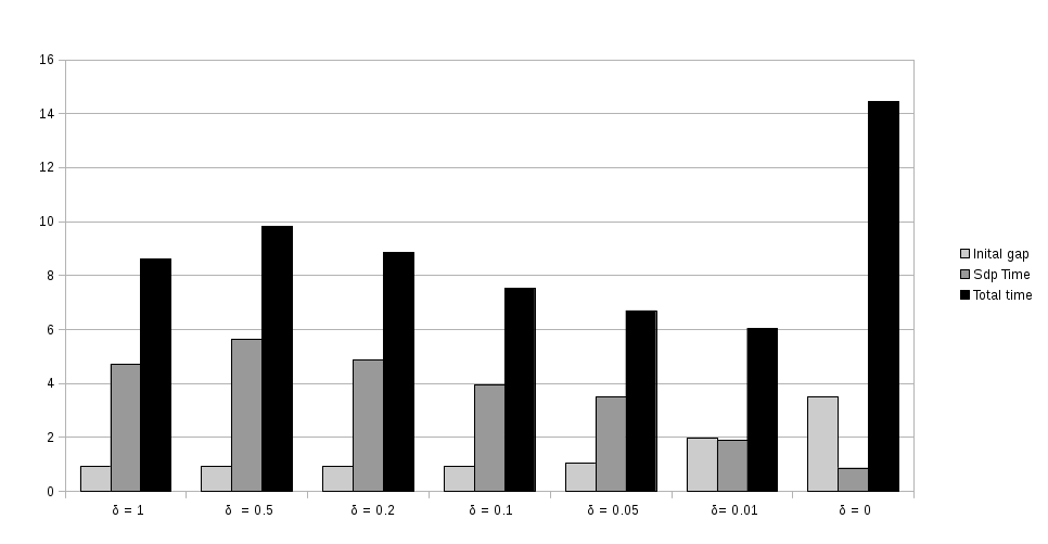
Figure 1: $k$-cluster instances of size $n=80$ : influence of parameter $p$

Experimental comparison of MIQCR-CB (with $p=4{n\choose 2}$) and MIQCR where Phase 1 is solved with CSDP turned into a heuristic

In this paper, we want to accelerate Phase 1 of our algorithm, and furthermore get an equivalent formulation with a reasonable size. A way to do this using interior-point algorithm for solving $(SDP)$ is to stop the solver CSDP with a much smaller precision and to consider the $\beta$ equals to zero with a much smaller precision. As instances of size $n=80$ are not practical for CSDP, we make experiments using instances of smaller size ($n=40$). We use 3 configurations for solving Phase 1 of our method:

• Configuration 1: We use CSDP turned into a heuristic: parameters axtol and aytol are set to $10^{-4}$ and parameter objtol is set to $10^{-1}$, and the tolerance for parameters $\beta_{ij}$ to be considered as non-zero to $10^{-4}$.

• Configuration 2: We use CSDP turned into a heuristic: parameters axtol, aytol are set to $10^{-4}$ and objtol is set to $10^{-1}$, and the tolerance for parameters $\beta_{ij}$ to be considered as non-zero to $10^{-2}$.

• Configuration 3: We use Algorithm 1: the stopping criteria is set to $10^{-4}$, and the tolerance for parameters $\beta_{ij}$ to be considered as non-zero to $10^{-4}$. We set $p$ to $4{n\choose 2}$.

We report in Table 3 the average number of variables $y_{ij}$ created in Phase 2 for each considered configuration of Phase 1. We recall that for these instances the maximum number of variables $y_{ij}$ created is 820.

Config. for Phase 1	nb $y_{ij}$ in Phase 2
Configuration 1	738
Configuration 2	554
Configuration 3	409

Table 3: Average number of variables $y_{ij}$ considered in Phase 2 of our algorithm

We report in Figure 2 the results obtained for the initial gap, the solution time of Phase 1, and the total solution time. In this graphic, the scale is logarithmic. We observe that the initial gap obtained with configuration 3 is about 22 times smaller than the initial gap obtained by configurations 1 and 2. Moreover, the solution time of Phase 1 is 68 times smaller for configuration 3, in comparison to configurations 1 and 2.

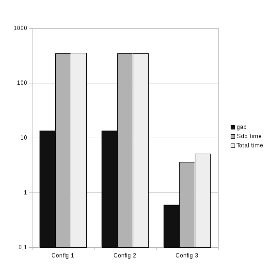
Figure 2: $k$-cluster instances of size $n=40$ : comparison with CSDP turned into a heuristic

Experiments to show the limitations of interior-points methods for solving problems with a huge number of constraints were already done in [19] and revealed a similar trend as ours.

Comparison of MIQCR-CB and BiqCrunch

In Table 4 we report computational results on instances of larger size, namely $n\in\{100,120,140,160\}$. For these instances, we compare method MIQCR-CB with BiqCrunch run on the same computer.

For instances of size $n=100$ and $n=120$, we observe that MIQCR-CB is as fast as BiqCrunch. Indeed, MIQCR-CB solves all $45$ instances of size $n=100$ ($n=120$ resp.) within $37.44$ ($370.89$ resp.) seconds on average, while BiqCrunch solves all the instances within $34.53$ ($338.07$ resp.) seconds. Notice that the initial gap is $1.6$ ($1.5$ resp.) times tighter for BiqCrunch than for MIQCR-CB. The average number of nodes is $1003$ ($1834$ resp.) times larger for MIQCR-CB for instances of size $n=100$ ($n=120$ resp.).

For the largest instances, namely those of size $n=140$ ($n=160$ resp.), MIQCR-CB is able to solve 38 (26 resp.) instances out of 45 within the time limit of 3 hours while BiqCrunch solves 43 (33 resp.) instances within 3 hours. The average computation time is 1973 (2081 resp.) seconds for MIQCR-CB and 1475 (1905 resp.) seconds for BiqCrunch. The initial gap is $1.4$ ($1.3$ resp.) times tighter for BiqCrunch than for MIQCR-CB. These largest instances represent the limit of both algorithms.

			MIQCR-CB ($p=4{n\choose 2}$)							BiqCrunch
n	d (%)	k	Gap	P1	P2	Tt	Min	Max	Nodes	Gap	Tt	Min	Max	Nodes
100	25	25	3.30	14.4	25.2	39.6	19	82	11964	1.78	71.3	14	265	26
100	25	50	0.84	13.6	9.8	23.4	17	44	3407	0.28	9.3	2	29	4
100	25	75	0.08	11.8	5.2	17	16	18	5	0.11	2.6	2	3	1
100	50	25	2.50	13.6	41.2	54.8	21	116	29116	1.76	59.4	19	140	33
100	50	50	0.90	17.2	87.8	105	18	176	77626	0.43	83.3	3	149	28
100	50	75	0.08	14.4	6.2	20.6	16	28	91	0.06	3.9	2	11	1
100	75	25	1.37	13.6	21.4	35	23	54	12559	1.19	75.1	44	116	43
100	75	50	0.35	13.8	10.2	24	19	31	3603	0.10	3.3	2	7	1
100	75	75	0.04	11.8	5.8	17.6	17	19	31	0.03	2.6	2	5	1
120	25	30	3.53	31.2	334.8	366	168	818	140208	2.22	348.5	224	522	104
120	25	60	1.03	33.4	343	376.4	75	695	151256	0.53	285.3	52	582	69
120	25	90	0.10	29	9.8	38.8	34	48	37	0.03	9.2	4	17	2
120	50	30	2.53	29.2	444.8	474	208	867	232762	1.92	581.9	251	1161	186
120	50	60	0.81	32.6	601.2	633.8	310	1246	322930	0.41	360.4	249	446	85
120	50	90	0.14	34	56.2	90.2	50	160	2895	0.08	135.1	38	301	22
120	75	30	1.57	31.6	791.6	823.2	56	2922	576795	1.42	1124.9	74	3232	403
120	75	60	0.47	40.4	457.8	498.2	111	903	245271	0.21	193.4	66	392	40
120	75	90	0.04	29	8.4	37.4	32	46	79.4	0.02	4.2	3	6	1.00
140	25	35	3.55	53.6	4458	4511.6	452	9940	1624107	2.41	1691.7	305	3493	349
140	25	70	1.07	61.2	2725.4	2786.6	221	7939	1124785	0.57	864.6	129	2456	143
140	25	105	0.09	46.2	15.6	61.8	51	75	134	0.04	19.2	5	25	3
140	50	35	2.61	54.3	3591.3(4)	3645.5 (4)	1262	7062	1501072	2.16	1958.9 (4)	806	3589	493
140	50	70	0.89	42	1871(1)	1913 (1)	1913	1913	1013112	0.54	4663.7	379	8763	800
140	50	105	0.08	50	43.8	93.8	54	151	1462	0.04	91.9	7	251	11
140	75	35	1.69	51.7	3748.3(3)	3800 (3)	2000	7048	1924558	1.57	4289.9 (4)	2475	9031	1128
140	75	70	0.39	54.4	1667.8	1722.2	493	4843	700401	0.19	305.9	185	551	46
140	75	105	0.05	47.2	193.2	240.4	47	721	9100.6	0.03	49.2	4	140	6
160	25	40	3.27	78.4	3932.7 (3)	4009.3 (3)	1705	7986	769425	2.29	2874.2 (4)	829	7078	453
160	25	80	1.02	77.5	4049(2)	4126.5(2)	2117	6136	811861	0.60	2737.7	491	6662	357
160	25	120	0.16	84.4	256.4	340.8	71	739	8872	0.09	353.1	38	899	31
160	50	40	2.54	69	9845(1)	9914(1)	9914	9914	2768184	2.15	6041.1(2)	5103	6979	1037
160	50	80	0.66	83	4665(2)	4748(2)	2182	7314	982063	0.42	4058(4)	558	9369	536
160	50	120	0.08	78.8	220.2	299	86	264	4222	0.04	212.5	41	468	16
160	75	40	1.68	110	3483(1)	3593(1)	3593	3593	871354	1.55	4518(1)	4518	4518	657
160	75	80	0.46	88.5	2176(2)	2264.5(2)	379	4150	403871	0.29	643.0(2)	84	1202	40
160	75	120	0.05	66.8	553	619.8	100	1392	12461	0.03	151.4	42	281	12

(i): i instances out of 5 were solved within the time limit. The reported values correspond to these instances.

Table 4: Average computational results of MIQCR-CB and BiqCrunch for 180 instances of the $k$-cluster of size $n=100$, $120$, $140$ and $160$ (time limit: 10 800 seconds).

4.2 Computational results on the general integer case

In this section we extend our computational experiments to the class of (general) quadratic integer problems to compare the improvement of MIQCR-CB over MIQCR on this more general class of instances, and evaluate our method with the state-of-the-art solvers Cplex12.6 [30] and Couenne [5]. We briefly recall that the solver Couenne [5] uses linear relaxations within a spatial branch-and-bound algorithm [6], and that Cplex12.6 uses a branch-and-bound algorithm based on convex relaxations [11]. For both solvers, numerous heuristics are incorporated into branch-and-bound algorithms in order to improve their performances.

Parameters:

• Parameters axtol, aytol of CSDP [13] are set to $10^{-8}$. The precision of the Conic Bundle [26] is set to $10^{-8}$. For method MIQCR-CB, we allow to dualize all constraints (i.e. $p=4{n\choose 2}$).

• Phase 2: A parameter $\beta_{ij}$ is considered as $0$ if $|\beta_{ij}|$ is below $10^{-6}$. For Cplex12.5 [29], the relative mipgap is $10^{-8}$ and the absolute gap is $0.99$. The parameter objdiff is set to $0.999$, and the parameter varsel to $4$. We used the multi-threading version of Cplex12.5 and Cplex12.6 with up to 8 threads. For solvers Cplex 12.6 and Couenne we keep the default parameters.

Experiments on the Equality Integer Quadratic Problem

We consider the Equality Integer Quadratic Problem (EIQP) that consists in minimizing a quadratic function subject to one linear equality constraint:

$$(EIQP) \min f(x)=\displaystyle{\sum_{i=1}^{n}}\displaystyle{\sum_{j=i}^{n}}q_{ij}x_{i}x_{j}+\sum_{i=1}^{n}c_{i}x_{i}$$

$$(EIQP)$$ s.t.

$$(EIQP) \quad\displaystyle{\sum_{i=1}^{n}}a_{i}x_{i}=b$$

$$(EIQP) \quad 0\leq x_{i}\leq u_{i} 1\leq i\leq n$$

$$(EIQP) \quad x_{i}\in\mathbb{N} 1\leq i\leq n$$

We use the instances introduced in [8], available online [38]. We run experiments on two classes of problem, EIQP_1 and EIQP_2. For each class we generate instances with $20$, $30$, and $40$ variables where the coefficients are randomly generated as follows:

• The coefficients of $Q$ and $c$ are uniformly distributed integers from the interval $[-100,100]$.

• The $a_{i}$ coefficients are uniformly distributed integers from the interval $[1,50]$ for class 1 and from $[1,100]$ for class 2.

• $b=\mu\cdot\displaystyle{\sum_{i=1}^{n}}a_{i}$, where $\mu=15$ for class 1 and $\mu=20$ for class 2.

• $u_{i}=30$ for $1\leq i\leq n$ for class 1, and $u_{i}=50$ for class 2.

For each class and each $n\in\{20,30,40\}$ we consider $5$ instances obtaining a set of $30$ instances in total. Each of these instances has at least one feasible solution ($x_{i}=\mu$ for all $i$). In Table 5 each line presents the results for one instance, $n$ indicates the size of the problem and $r$ the reference of the instance within the 5 instances with the same characteristics. The other columns are as described in Legends of Tables 1 and 4–6. We use the same experimental environment as described in Section 4.1.

			MIQCR					MIQCR-CB $(p=4{n\choose 2})$					Cplex12.6			Couenne
class	n	r	Gap	P1	P2	Tt	Nodes	Gap	P1	P2	Tt	Nodes	Gap	Tt	Nodes	Tt	Nodes
EIQP_1	20	1	0.1	26	115	141	3956	0.1	2	37	39	1252	159	2	2000	16	2044
EIQP_1	20	2	0.1	15	15	30	5	0.1	2	12	14	11	178	1	817	5	342
EIQP_1	20	3	0.1	20	8	28	0	0.1	3	13	16	75	177	2	1000	16	1990
EIQP_1	20	4	0.0	23	4	27	0	0.0	3	3	6	0	144	1	69	4	56
EIQP_1	20	5	0.2	26	16	42	43	0.2	3	25	28	255	209	2	2000	8	475
EIQP_1	30	1	0.0	289	108	397	80	0.0	14	45	59	142	182	25	8000	1644	116242
EIQP_1	30	2	0.0	184	11	195	0	0.0	14	25	39	1	175	13	3500	347	16938
EIQP_1	30	3	0.0	216	384	600	2741	0.0	37	59	96	218	183	33	13500	179	9714
EIQP_1	30	4	0.1	218	68	286	23	0.1	19	23	42	26	160	218	53500	1231	53330
EIQP_1	30	5	0.1	200	248	448	1251	0.1	20	92	112	1352	159	223	84000	596	33841
EIQP_1	40	1	0.0	1093	2234	3327	1816	0.0	17	237	254	296	175	13	3000	148	1925
EIQP_1	40	2	0.0	1219	452	1671	558	0.0	220	254	474	233	161	432	56000	failed
EIQP_1	40	3	0.0	1325	196	1521	0	0.0	67	78	145	2	172	(10$\%$)	259500	failed
EIQP_1	40	4	0.0	1672	870	2542	3226	0.0	1239	157	1396	799	169	2382	258000	(2$\%$)	87323
EIQP_1	40	5	0.2	2281	863	3144	3871	0.2	1362	622	1984	6365	163	(9$\%$)	294000	(14$\%$)	84268
EIQP_2	20	1	0.1	23	66	89	2583	0.1	3	112	115	7979	159	2	2000	39	5585
EIQP_2	20	2	0.0	60	10	70	3	0.0	10	12	22	11	180	3	3500	21	1748
EIQP_2	20	3	0.0	30	17	47	73	0.0	2	18	20	140	138	1	500	5	336
EIQP_2	20	4	0.2	32	54	86	1726	0.2	7	56	63	2777	155	2	3000	16	2132
EIQP_2	20	5	0.1	19	31	50	341	0.1	6	45	51	1590	588	4	5000	9	724
EIQP_2	30	1	0.3	481	494	975	4237	0.3	1296	165	1461	2011	186	86	50000	287	14978
EIQP_2	30	2	0.1	337	256	593	1488	0.1	6	282	288	45378	171	21	13500	92	4655
EIQP_2	30	3	0.0	264	201	465	1009	0.0	44	105	149	893	160	159	125000	284	15589
EIQP_2	30	4	0.1	180	667	847	3728	0.1	6	226	232	4255	134	9	6000	86	4440
EIQP_2	30	5	0.1	476	398	874	3591	0.1	1161	100	1261	1737	160	169	70000	413	24752
EIQP_2	40	1	0.0	1078	1137	2215	739	0.0	33	750	783	2610	160	1739	236000	1387	39258
EIQP_2	40	2	0.1	1216	2295	3511	4876	0.1	28	989	1017	5473	216	(11$\%$)	535500	(15$\%$)	82426
EIQP_2	40	3	0.1	1118	2180	3298	3275	0.1	17	1238	1255	6664	166	1366	253000	3016	95223
EIQP_2	40	4	0.0	1306	165	1471	0	0.0	25	84	109	5	162	7	1500	80	391
EIQP_2	40	5	0.0	2234	1415	3649	3616	0.0	67	697	764	2841	177	(6$\%$)	450000	failed

Table 5: Computational results of MIQCR-CB, MIQCR, Cplex12.6 and Couenne for 30 general integer instances with $20$, $30$ and $40$ variables of classes EIQP_1 and EIQP_2 (B&B time limit: 3 600 seconds).

The numerical results comparing methods MIQCR-CB, MIQCR, Cplex12.6 and Couenne are given in Table 5. We observe that both algorithms MIQCR-CB and MIQCR solve all considered instances in less than $3\,649$ seconds of cpu time, while Cplex12.6 solves only $26$ instances and Couenne only 24 instances, over the $30$ considered instances in less than one hour of cpu time. Comparing MIQCR and MIQCR-CB, we observe that MIQCR-CB is always faster than MIQCR. More precisely, while the initial gap remains the same for both methods, for class EIQP_1 (EIQP_2 resp.) the solution time for Phase 1, for MIQCR-CB in comparison to MIQCR, is divided on average by a factor of about $2.9$ ($3.3$ resp.), and by a factor $3.3$ ($1.9$ resp.) for the solution time of Phase 2. Hence the total run time significantly decreases (factor $3.1$ for EIQP_1 and $2.4$ for EIQP_2). Comparing Cplex12.6 and Couenne with MIQCR-CB, we observe that Cplex12.6 and Couenne are often faster than MIQCR-CB for the smallest considered instances, but with increasing dimension, MIQCR-CB is superior to Cplex12.6 and Couenne. Moreover, we can notice a significant decrease of the initial gap with method MIQCR-CB (by a factor $2600$) and of the number of visited nodes during the branch-and-bound algorithm (by a factor $180$ and $90$), in comparison to Cplex12.6 and Couenne.

Experiments on the Integer Equipartition Problem

We consider the Integer Equipartition Problem (IEP). This problem is an extension of the classical min-cut graph problem which consists in partitioning the vertices of a graph into a collection of disjoint sets satisfying specified size constraints, while minimizing the sum of weights of edges connecting vertices in different sets [22]. In (IEP) we consider $n$ types of items, $m$ items of each type, and a partition of the $n\cdot m$ items into $p$ equally sized sets. We assume that $n\cdot m$ is a multiple of $p$. For all pairs of type of items $(i,j),\,\,i\leq j$, we denote by $c_{ij}$ the cost of allocating each pair of items of types $i$ and $j$ to different sets. The problem consists thus to minimize the total cost of allocating the $n\cdot m$ items to the $p$ sets. By introducing decision variables $x_{ik}$ which represent the number of items of type $i$ allocated to set $k$, (IEP) can be formulated as follows:

$$(IEP) \min\,\,\displaystyle{\sum_{i<j}}\displaystyle{\sum_{k\neq l}}c_{ij}x_{ik}x_{jl}+\displaystyle{\sum_{i}}\displaystyle{\sum_{k<l}}c_{ii}x_{ik}x_{il}$$

$$(IEP)$$ s.t.

$$(IEP) \quad\displaystyle{\sum_{i=1}^{n}}x_{ik}=\frac{n\cdot m}{p} 1\leq k\leq p$$ (32)

$$(IEP) \quad\displaystyle{\sum_{k=1}^{p}}x_{ik}=m 1\leq i\leq n$$ (33)

$$(IEP) \quad 0\leq x_{ik}\leq\min(m,\frac{n\cdot m}{p}) 1\leq i\leq n 1\leq k\leq p$$ ,  (34)

$$(IEP) \quad x_{ik}\in\mathbb{N} 1\leq i\leq n 1\leq k\leq p$$ ,  (35)

where Constraints (32) ensure that exactly $\frac{n\cdot m}{p}$ items are allocated to each set, Constraints (33) ensure that all items are allocated to a set. This problem has a quadratic objective function, $n+p$ linear equalities and $n\cdot p$ general integer variables.

We generate instances of (IEP) with $n=3$ or $4$, $m=20$ or $24$ and $p=5$ or $6$, where the coefficients $c$ are uniformly distributed integers from the interval $[1,10]$. For each characteristics, we generate 10 instances. The numerical results comparing methods MIQCR-CB, Cplex12.6 and Couenne are given in Table 6 where each line presents the results for one instance, $n$ indicates the number of types of items, $m$ the number of items of each type, $p$ the number of equally sized sets, and $r$ the reference of the instance within the 10 instances with the same characteristics. The other columns are as described in Legends of Tables 1 and 4–6

				MIQCR-CB $p=(4{n\choose 2})$					Cplex12.6			Couenne
n	m	p	r	Gap	P1	P2	Tt	Nodes	Gap	Tt	Nodes	Tt	Nodes
03	20	05	1	0.00	0	16	16	0	90.87	(5.07$\%$)	3054000	2888	1074696
03	20	05	2	0.00	0	2	2	0	76.64	546	2244000	(1.4$\%$)	1271760
03	20	05	3	2.07	1	110	111	29966	78.21	606	2487500	317	122622
03	20	05	4	1.50	1	38	39	8990	76.31	552	2244000	309	118438
03	20	05	5	1.73	0	13	13	2457	95.76	(2.17$\%$)	2875500	663	231750
03	20	05	6	0.11	1	13	14	1507	81.73	(8.24$\%$)	3272500	(2.1$\%$)	1182335
03	20	05	7	1.01	1	23	24	7481	97.8	(5.8$\%$)	3158000	2143	744678
03	20	05	8	0.11	9	8	17	571	81.6	(5.17$\%$)	3009000	1122	424302
03	20	05	9	0.12	1	13	14	1815	94.24	(4.73$\%$)	2951000	1534	595765
03	20	05	10	0.14	1	9	10	864	88.09	(5.07$\%$)	3054000	2194	814563
03	24	06	1	0.00	1	5	6	0	88.2	(16.88$\%$)	2636000	(12.5$\%$)	661600
03	24	06	2	0.00	0	4	4	0	87.11	(18.6$\%$)	2575500	(14.1$\%$)	659827
03	24	06	3	0.00	1	7	8	29	80.19	(10.46$\%$)	2604500	(3.4$\%$)	721369
03	24	06	4	0.00	1	9	10	321	83.39	(11.17$\%$)	2501500	(3.8$\%$)	745568
03	24	06	5	0.00	5	3	8	0	84.66	(12.63$\%$)	2543500	(6.5$\%$)	713247
03	24	06	6	0.02	1	34	35	1943	88.75	(18.1$\%$)	2611500	(14.8$\%$)	650991
03	24	06	7	0.00	4	2	6	0	86.81	(15.61$\%$)	2503500	(10.8$\%$)	667285
03	24	06	8	0.35	20	241	261	31505	84.27	(14.99$\%$)	2582000	(11.5$\%$)	647872
03	24	06	9	0.04	11	7	18	309	77.35	(15.64$\%$)	2522000	(11.7$\%$)	693954
03	24	06	10	0.07	73	25	98	1754	79.58	(16.06$\%$)	2574000	(12.5$\%$)	662087
04	20	05	1	0.37	39	(0.18$\%$)	-	185288	94.02	(24.69$\%$)	1925000	(31.7$\%$)	546677
04	20	05	2	1.84	97	(1.26$\%$)	-	190884	91.46	(22.58$\%$)	1964500	(24.8$\%$)	571394
04	20	05	3	2.42	72	(1.83$\%$)	-	176167	86.75	(19.82$\%$)	2018500	(24.2$\%$)	590082
04	20	05	4	0.09	8	144	152	4714	90.17	(24.84$\%$)	1908500	(32.2$\%$)	528364
04	20	05	5	3.82	79	(2.33$\%$)	-	155941	90.05	(16.85$\%$)	2036500	(15.9$\%$)	630677
04	20	05	6	0.06	131	129	260	4454	84.43	(26.29$\%$)	1924500	(33.1$\%$)	518391
04	20	05	7	0.62	89	(0.46$\%$)	-	217944	87.1	(27.58$\%$)	1923000	(36.9$\%$)	496121
04	20	05	8	0.05	47	96	143	3942	97.29	(27.02$\%$)	1901500	(31.8$\%$)	512563
04	20	05	9	1.50	102	(1.15$\%$)	-	188395	95.93	(21.16$\%$)	199250	(24.6$\%$)	5764810
04	20	05	10	1.41	351	(1.27$\%$)	-	141855	91.96	(25.06$\%$)	1903000	(27.1$\%$)	557275
04	24	06	1	0.06	102	(0.06$\%$)	-	74597	93.62	(42.69$\%$)	1193500	(72.3$\%$)	308012
04	24	06	2	1.26	113	(1.12$\%$)	-	79635	90.36	(43.71$\%$)	1210500	(65.1$\%$)	314582
04	24	06	3	1.26	93	(1.09$\%$)	-	70921	93.48	(36.72$\%$)	1252500	(61.7$\%$)	336893
04	24	06	4	0.03	15	721	736	13603	99.26	(43.95$\%$)	1227000	(74.9$\%$)	298315
04	24	06	5	2.96	107	(2.29$\%$)	-	66534	94.02	(40.12$\%$)	1251000	(58.5$\%$)	340087
04	24	06	6	0.01	189	66	255	829	93.13	(45.61$\%$)	1224500	(74.2$\%$)	299641
04	24	06	7	0.00	136	353	489	6261	95.88	(43.85$\%$)	1199500	(71.5$\%$)	295719
04	24	06	8	0.25	16	(0.21$\%$)	-	118263	99.65	(48.48$\%$)	1218500	(75.0$\%$)	301299
04	24	06	9	0.01	151	260	411	3903	95.21	(42.23$\%$)	1194500	(60.3$\%$)	324965
04	24	06	10	0.85	1648	(0.81$\%$)	-	79072	92.82	(44.19$\%$)	1171500	(66.3$\%$)	315380

Table 6: Computational results of MIQCR-CB, Cplex12.6 and Couenne for 40 instances of (IEP) (time limit: 3 600 seconds)

We observe that MIQCR-CB is able to solve $27$ of the $40$ considered instances, while Cplex12.6 solves only $3$ instances and Couenne 8 instances of the 10 of the smallest size. Moreover these 3 (8 resp.) instances are solved by Cplex12.6 (Couenne resp.) within 568 (1396 resp.) seconds in average, while MIQCR-CB solves the 10 instances within 27 seconds on average. An important advantage of MIQCR-CB is its gap that is on average 136 times smaller than the gap of Cplex12.6, and that is moreover quite stable independently from the characteristics of the instances.

5 Conclusion

We presented algorithm MIQCR-CB for solving general integer quadratic programs with linear constraints. This algorithm is an improvement of MIQCR [8]. MIQCR-CB is an approach in two phases: the first phase calculates an equivalent quadratic reformulation of the initial problem by solving a semidefinite program, and the second phase solves the reformulated problem using standard mixed-integer quadratic programming solver.

In Phase 1, a subgradient algorithm within a Lagrangian duality framework is used to solve the semidefinite program that yields the parameters for constructing an equivalent (convex) formulation. This significantly speeds up Phase 1 compared to the earlier method MIQCR. Furthermore, by construction, we can control the size of the reformulated problem. As a consequence, Phase 2 of our algorithm is also accelerated. Thus, MIQCR-CB builds a reformulated problem with a tight bound that can be computed in reasonable time, even for large instances.

Computational experiments carried out on the $k$-cluster problem demonstrate that our method is competitive with the best current approaches devoted to the solution of this binary quadratic problems for instances with up to $120$ variables. Moreover, our approach is able to solve most of the instances with $160$ variables to optimality within 3 hours of cpu time. We also demonstrate that MIQCR-CB outperforms MIQCR, Cplex12.6 and Couenne on two classes of general integer quadratic problems, which confirms the impact of the newly designed procedure for solving the SDP.

Acknowledgment: We thank Franz Rendl for useful discussions and two anonymous referees for suggestions that improved this paper.

References

- [1] K. M. Anstreicher. Semidefinite programming versus the reformulation-linearization technique for nonconvex quadratically constrained quadratic programming. Journal of Global Optimization, 43:471–484, 2009.
- [2] Y. Asahiro, K. Iwama, H. Tamaki, and T. Tokuyama. Greedily finding a dense subgraph. In Proceedings of the 5th Scandinavian Workshop on Algorithm Theory. Lectures notes in Computer Science, 1097, Springer-Verlag, pages 136–148, 1996.
- [3] C. Audet, P. Hansen, B. Jaumard, and G. Savard. A branch and cut algorithm for non-convex quadratically constrained quadratic programming. Mathematical Programming, 87(1):131–152, 2000.
- [4] Alexandre Belloni and Claudia Sagastizábal. Dynamic bundle methods. Math. Program., 120(2, Ser. A):289–311, 2009.
- [5] P. Belotti. Couenne, a user’s manual. ”http://www.coin-or.org/Couenne/”, 2013.
- [6] P. Belotti, J. Lee, L. Liberti, F. Margot, and A. Wächter. Br anching and bounds tightening techniques for non-convex minlp. Optimization Methods and Software, 4–5(24):597–634, 2009.
- [7] A. Billionnet. Different formulations for solving the heaviest -subgraph problem. Information Systems and Operational Research, 3(43):171–186, 2005.
- [8] A. Billionnet, S. Elloumi, and A. Lambert. Extending the QCR method to the case of general mixed integer program. Mathematical Programming, 131(1):381–401, 2012.
- [9] A. Billionnet, S. Elloumi, and M.-C. Plateau. Convex quadratic programming for exact solution of 0-1 quadratic programs. Technical Report CEDRIC-05-856, CEDRIC, 2005.
- [10] A. Billionnet, S. Elloumi, and M.-C. Plateau. Improving the performance of standard solvers for quadratic 0-1 programs by a tight convex reformulation: the QCR method. Discrete Applied Mathematics, 0(157):1185–1197, 2009.
- [11] C. Bliek and P. Bonami. Non-convex quadratic programming in cplex. INFORMS 2013 Annual Meeting, 2013.
- [12] P. Bonami, L. Biegler, A. Conn, G. Cornuéjols, I. Grossmann, C. Laird, J. Lee, A. Lodi, F. Margot, N. Sawaya, and A. Waechter. An algorithmic framework for convex mixed integer nonlinear programming. Discrete Optimization, 5:186–204, 2005.
- [13] B. Borchers. CSDP, a C library for semidefinite programming. Optimization Methods and Software, 11(1):613–623, 1999.
- [14] S. Burer and R.D.C. Monteiro. A nonlinear programming algorithm for solving semidefinite programs via low-rank factorization. Math. Program., 95(2, Ser. B):329–357, 2003. Computational semidefinite and second order cone programming: the state of the art.
- [15] S. Burer and R.D.C. Monteiro. Local minima and convergence in low-rank semidefinite programming. Math. Program., 103(3, Ser. A):427–444, 2005.
- [16] D.G. Corneil and Y.A. Perl. Clustering and domination in perfect graphs. Discrete Applied Mathematics, 9(1):27–39, 1984.
- [17] B. Le Cun, C. Roucairol, and The PNN Team. A unified platform for implementing branch-and-bound like algorithms, 1995.
- [18] E. Erkut. The discrete -dispersion problem. European Journal of Operational Research, 46:46–80, 1990.
- [19] I. Fischer, G. Gruber, F. Rendl, and R. Sotirov. Computational experience with a bundle approach for semidefinite cutting plane relaxations of Max-Cut and equipartition. Mathematical Programming, 105:451–469, 2006.
- [20] C. A. Floudas. Deterministic global optimization. Kluwer Academic Publishing, Dordrecht, The Netherlands, 2000.
- [21] K. Fujisawa and M. Kojima. SDPA (semidefinite programming algorithm) users manual. Technical Report B-308, Tokyo Institute of Technology, 1995.
- [22] W.W. Hager and Y. Krylyuk. Graph partitioning and continuous quadratic programming. SIAM Journal on Discrete Mathematics, 12:500–523, 1999.
- [23] Q. Han, Y. Ye, and J. Zhang. An improved rounded method and semidefinite programming relaxation for graph partition. Mathematical Programming, 92(3):509–535, 2002.
- [24] R. Hassin, S. Rubinstein, and A. Tamir. Approximation algorithms for maximum dispersion. Operations Research Letters, pages 133–137, 1997.
- [25] C. Helmberg. A C++ implementation of the spectral bundle method. Manual version 1.1.1, 2000.
- [26] C. Helmberg. Conic Bundle v0.3.10, 2011.
- [27] C. Helmberg and F. Rendl. A spectral bundle method for semidefinite programming. SIAM Journal of Optimization, 10(3):673–696, 2000.
- [28] Christoph Helmberg, Franz Rendl, Robert J. Vanderbei, and Henry Wolkowicz. An interior-point method for semidefinite programming. SIAM J. Optim., 6(2):342–361, 1996.
- [29] IBM-ILOG. Ibm ilog cplex 12.5 reference manual. ”http://pic.dhe.ibm.com/infocenter/cosinfoc/v12r2/index.jsp”, 2013.
- [30] IBM-ILOG. Ibm ilog cplex 12.6 reference manual. ”http://www-01.ibm.com/support/knowledgecenter/SSSA5P_12.6.0/ilog.odms.%studio.help/Optimization_Studio/topics/COS_home.html”, 2014.
- [31] G. Jäger and A. Srivastav. Improved approximation algorithms for maximum graph partitioning problems. Journal of Combinatorial Optimization, 10(2):133–167, 2005.
- [32] F. Jarre and F. Rendl. An augmented primal-dual method for linear conic programs. SIAM J. Optim., 19(2):808–823, 2008.
- [33] G. Kortsarz and D. Peleg. On choosing a dense subgraph. In Proceedings of the 34th Annual IEEE Symposium on Foundations of Computer Science, pages 692–701, 1993.
- [34] J. Krarup, D. Pisinger, and F. Plastria. Discrete location problems with push-pull objectives. Discrete Applied Mathematics, 123:363–378, 2002.
- [35] N. Krislock, J. Malick, and F. Roupin. Improved semidefinite branch-and-bound algorithm for -cluster. submitted, 2013.
- [36] N. Krislock, J. Malick, and F. Roupin. Library of -cluster instances. ”http://lipn.univ-paris13.fr/BiqCrunch/download”, 2013.
- [37] A. Lambert. Résolution de programmes quadratiques en nombres entiers. Thèse de doctorat en informatique, Conservatoire National des Arts et Métiers, Paris, 2009.
- [38] A. Lambert. EIQP/IIQP: Library of integer quadratic programs. ”http://cedric.cnam.fr/~lamberta/Library/eiqp_iiqp.html”, 2012.
- [39] L. Liberti and N. Maculan. Global optimization: From theory to implementation, chapter: Nonconvex optimization and its applications. Springer, New York, 2006.
- [40] J. Malick. Spherical constraint in boolean quadratic programming. Journal of Global Optimization, 39(4):609–622, 2007.
- [41] J. Malick, J. Povh, F. Rendl, and A. Wiegele. Regularization methods for semidefinite programming. SIAM J. Optim., 20(1):336–356, 2009.
- [42] Jérôme Malick and Frédéric Roupin. Solving -cluster problems to optimality with semidefinite programming. Math. Program., 136(2 (B)):279–300, 2012.
- [43] G.P. McCormick. Computability of global solutions to factorable non-convex programs: Part i - convex underestimating problems. Mathematical Programming, 10(1):147–175, 1976.
- [44] D. Pisinger. Upper bounds and exact algorithms for -dispersion problems. Computers and Operations Research, 33:1380–1398, 2006.
- [45] M.-C. Plateau. Reformulations quadratiques convexes pour la programmation quadratique en variables 0-1. Thèse de doctorat en informatique, Conservatoire National des Arts et Métiers, Paris, 2006.
- [46] F. Roupin. From linear to semidefinite programming: an algorithm to obtain semidefinite relaxations for bivalent quadratic problems. Journal of Combinatorial Optimization, 8(4):469–493, 2004.
- [47] N.V. Sahinidis and M. Tawarmalani. A polyhedral branch-and-cut approach to global optimization. Mathematical Programming, 103(2):225–249, 2005.
- [48] N.V. Sahinidis and M. Tawarmalani. Baron 9.0.4: Global optimization of mixed-integer nonlinear programs. User’s Manual, 2010.
- [49] E. M. B. Smith. On the optimal design of continuous processes. PhD thesis, Imperial College of Science, Technology and Medicine, University of London, 1996.
- [50] E. M. B. Smith and C. C. Pantelides. Global optimisation of nonconvex minlps. Computers and Chem. Engineering, 21:S791–S796, 1997.
- [51] E. M. B. Smith and C. C. Pantelides. A symbolic reformulation/spatial branch-and-bound algorithm for the global optimisation of nonconvex minlps. Computers and Chem. Engineering, 23:457–478, 1999.
- [52] A. Srivastav and K. Wolf. Finding dense subgraph with semidefinite programming. Approximation Algorithms for Combinatorial Optimization, K. Jansen and J. Rolim (Eds.), pages 181–191, 1998.
- [53] Jos F. Sturm. Using SeDuMi 1.02, a MATLAB toolbox for optimization over symmetric cones. Optim. Methods Softw., 11-12(1-4):625–653, 1999.
- [54] M. Tawarmalani and N.V. Sahinidis. Convexification and global optimization in continuous and mixed-integer nonlinear programming. Kluwer Academic Publishing, Dordrecht, The Netherlands, 2002.
- [55] X.-Y. Zhao, D. Sun, and K.-C Toh. A Newton-CG augmented Lagrangian method for semidefinite programming. SIAM J. Optim., 20(4):1737–1765, 2010.