Constraints on Scalar Leptoquark from Kaon Sector

Abstract

Recently, several anomalies in flavor physics have been observed, and it was noticed that leptoquarks might account for the deviations from the Standard Model. In this work, we examine the effects of new physics originating from a scalar leptoquark model on the kaon sector. The leptoquark we consider is a ${\rm\,Te\kern-1.25ptV}$-scale particle and within the reach of the LHC. We use the existing experimental data on the several kaon processes including $K^{0}-\bar{K}^{0}$ mixing, rare decays $K^{+}\rightarrow\pi^{+}\nu\bar{\nu}$, $K_{L}\rightarrow\pi^{0}\nu\bar{\nu}$, short-distance part of $K_{L}\rightarrow\mu^{+}\mu^{-}$, and lepton-flavor-violating decay $K_{L}\rightarrow\mu^{\pm}e^{\mp}$ to obtain useful constraints on the model.

I Introduction

The discovery of the last missing piece, the Higgs boson, in the first run of the LHC marks the completion of the Standard Model (SM) Aad:2012tfa ; Chatrchyan:2012xdj . Though the SM has been exceptionally successful in explaining the experimental data collected so far, there are many important questions which demand for physics beyond the SM (see, for example, Ricciardi:2015iwa ). Therefore, it is natural to consider the SM as the low-energy limit of a more general theory above the electroweak scale. The direct collider searches at the high-energy frontier ( TeV-scale) have not found any new particle but, interestingly, there are some tantalizing hints towards new physics (NP) from high-precision low-energy experiments in the flavor sector. To be specific, in 2012, BaBar measured the ratios of branching fractions for the semitauonic decay of the $B$ meson, $\bar{B}\rightarrow D^{\ast}\tau\bar{\nu}$,

$${\cal R}(D^{(\ast)})=\frac{{\rm BR}(\bar{B}\rightarrow D^{(\ast)}\tau\bar{\nu})}{{\rm BR}(\bar{B}\rightarrow D^{(\ast)}\ell\bar{\nu})},$$ (1)

with $\ell=e,\mu$, and reported $2.0\sigma$ and $2.7\sigma$ excesses over the SM predictions in the measurements of ${\cal R}(D)$ and ${\cal R}(D^{\ast})$, respectively Lees:2012xj . Very recently, these decays have been measured by BELLE Huschle:2015rga and LHCb Aaij:2015yra . These results are in agreement with each other and when combined together show a significant deviation from the SM. A summary of the measurements of ${\cal R}(D^{(\ast)})$ done by different collaborations together with the SM predictions is given in Table 1.

	${\cal R}(D^{\ast})$	${\cal R}(D)$
LHCb Aaij:2015yra	0.336 $\pm$ 0.027 $\pm$ 0.030	-
BaBar Lees:2012xj	0.332 $\pm$ 0.024 $\pm$ 0.018	0.440 $\pm$ 0.058 $\pm$ 0.042
BELLE Huschle:2015rga	0.293 $\pm$ 0.038 $\pm$ 0.015	0.375 $\pm$ 0.064 $\pm$ 0.026
SM Pred.Fajfer:2012vx	0.252 $\pm$ 0.003	0.300 $\pm$ 0.010

Table 1: Summary of experimental measurement for the ratios $R(D^{(\ast)})$ and the expectation in the SM. Here the first (second) errors are statistical (systematic).

Another interesting indirect hint of NP comes from the data on $b\rightarrow s\mu^{+}\mu^{-}$ processes. The LHCb Collaboration has seen a $2.6\sigma$ departure from the SM prediction in the lepton flavor universality ratio $R_{K}={\rm BR}(\bar{B}\rightarrow\bar{K}\mu^{+}\mu^{-})/{\rm BR}(\bar{B}\rightarrow\bar{K}e^{+}e^{-})=0.745^{+0.090}_{-0.074}\pm 0.036$ in the dilepton invariant mass bin $1{\rm\,Ge\kern-1.25ptV}^{2}<q^{2}<6{\rm\,Ge\kern-1.25ptV}^{2}$ Aaij:2014ora . Though the individual branching fractions for $\bar{B}\rightarrow\bar{K}\mu^{+}\mu^{-}$ and $\bar{B}\rightarrow\bar{K}e^{+}e^{-}$ are marred with large hadronic uncertainties in the SM Bobeth:2007dw , their ratio is a very clean observable and predicted to be $R_{K}=1.0003\pm 0.0001$ Hiller:2003js ; Bobeth:2007dw . Also, the recent data on angular observables of four-body distribution in the process $(B\rightarrow K^{*}(\rightarrow K\pi)\ell^{+}\ell^{-}$ indicate some tension with the SM Aaij:2013qta ; Aaij:2015oid , particularly the deviation of $\sim 3\sigma$ in two of the $q^{2}$ bins of angular observable $P_{5}^{{}^{\prime}}$ DescotesGenon:2012zf (also see Refs. Matias:2012xw ; Descotes-Genon:2013vna for discussion on other angular observables for $B\rightarrow K^{*}\ell^{+}\ell^{-}$ decay). In the decay $B_{s}\rightarrow\phi\mu^{+}\mu^{-}$, a deviation of $3.5\sigma$ significance with respect to the SM prediction has also been reported by LHCb Aaij:2015esa . The model-independent global fits to the data on $b\rightarrow s\mu^{+}\mu^{-}$ observables point towards a solution with NP that is favored over the SM by $\sim 4\sigma$ Descotes-Genon:2013wba ; Altmannshofer:2015sma ; Descotes-Genon:2015uva .

Several NP scenarios have been proposed to explain these discrepancies. The excesses in ${\cal R}(D^{(\ast)})$ have been explained in a generalized framework of 2HDM in Refs. Celis:2012dk ; Ko:2012sv ; Crivellin:2012ye , in the framework of the $R$-parity violating Minimal Supersymmetric Standard Model in Ref. Deshpande:2012rr , in the $E_{6}$-motivated Alternative Left-Right Symmetric Model (ALRSM) in Ref. Hati:2015awg , and using a model-independent approach Datta:2012qk ; Bhattacharya:2015ida ; Tanaka:2012nw ; Freytsis:2015qca , while in Refs. Dorsner:2009cu ; Fajfer:2012jt ; Sakaki:2013bfa ; Dorsner:2013tla the excesses in ${\cal R}(D^{(\ast)})$ have been addressed in the context of leptoquark models. The possible explanation for the observed anomalies in $b\rightarrow s\mu^{+}\mu^{-}$ processes preferably demands a negative contribution to the Wilson coefficient of semileptonic operator $(\bar{s}b)_{\rm V-A}(\bar{\mu}\gamma_{\alpha}\mu)$ Blake:2015tda ; Altmannshofer:2015sma . Several NP models, generally involving $Z^{{}^{\prime}}$ vector bosons Gauld:2013qja ; Glashow:2014iga ; Crivellin:2015lwa ; Altmannshofer:2014cfa ; Buras:2013qja ; Crivellin:2015mga ; Chiang:2016qov ; Boucenna:2016wpr or leptoquarks Gripaios:2014tna ; Becirevic:2015asa ; Alonso:2015sja ; Calibbi:2015kma ; Bauer:2015knc ; Barbieri:2015yvd ; Varzielas:2015iva ; Fajfer:2015ycq ; Hiller:2014yaa , are able to produce such operators with the required effects to explain the present data.

In view of this, we are motivated to study a ${\rm\,Te\kern-1.25ptV}$-scale leptoquark model and analyze NP effects on the kaon sector. It is known that the studies of kaon decays have played a vital role in retrieving information on the flavor structure of the SM. In particular, neutral kaon mixing and the rare decays of the kaon have been analyzed in various extensions of the SM and are known to provide some of the most stringent constraints on NP Buras:2013ooa ; Blanke:2013goa ; Buras:1997ij ; Buras:2012ts ; Buras:2004qb ; Blanke:2009am ; Blanke:2008yr ; Bauer:2009cf ; Buras:2012dp ; Buras:2014yna ; Queiroz:2014pra ; Lee:2015qra ; Mescia:2012fg . The NP model we consider in this paper is a simple extension of the SM by a single scalar leptoquark. The leptoquark $\phi$ with mass $M_{\phi}$ has $(SU(3),\,SU(2))_{U(1)}$ quantum numbers $(3,1)_{-1/3}$. This model is interesting considering that it has all the necessary ingredients accommodating semileptonic $b\rightarrow c$ and $b\rightarrow s$ decays to explain the anomalies in the LFU ratios discussed above Bauer:2015knc ; Hiller:2014yaa . To this end, we must mention that, along with anomalies observed in the flavor sector, the leptoquark model under study is also capable of explaining the new diphoton excess recently reported by the ATLAS and CMS collaborations in their analysis of $\sqrt{s}=13{\rm\,Te\kern-1.25ptV}$ $pp$ collision diphoton excess ref .

Following the conventions of Ref. Bauer:2015knc , the Lagrangian governing the leptoquark interaction with first-family fermions is given by

$${\cal L}^{(\phi)}\ni\lambda^{L}_{ue}\bar{u}^{c}_{L}e_{L}\phi^{*}+\lambda^{R}_{ue}\bar{u}^{c}_{R}e_{R}\phi^{*}-\lambda^{L}_{d\nu}\bar{d}^{c}_{L}\nu_{L}\phi^{*}+h.c.,$$

where L/R are the left/right projection operators $(1\mp\gamma_{5})/2$. The couplings $\lambda$’s are family dependent, and $u^{c}$=$C\bar{u}^{T}$ are the charge-conjugated spinors. Similar interaction terms for the second and third families can also be written down. In this model, $B\rightarrow D^{(\ast)}\tau\bar{\nu}$ proceeds at tree level through the exchange of leptoquark $(\phi)$. Integrating out the heavy particles gives rise to low-energy dimension-six effective operators, which can produce the required effects to satisfy the experimental data. In Ref. Bauer:2015knc , it was shown that with $O(1)$ left-handed and relatively suppressed right-handed couplings one can explain the observed excesses in the rate of $B\rightarrow D^{(\ast)}\tau\bar{\nu}$ decays. The authors of Ref. Bauer:2015knc were also able to simultaneously explain the observed anomalies in $R_{K}$ with large $(\sim O(1))$ left-handed couplings for a ${\rm\,Te\kern-1.25ptV}$-scale leptoquark. In this model, such large couplings are possible because the leading contribution to $\bar{B}\rightarrow\bar{K}\mu^{+}\mu^{-}$ comes from one-loop diagrams and therefore additional GIM and CKM suppression compensates for the “largeness” of the couplings. This is in contrast to NP models Hiller:2014yaa ; Sahoo:2015wya ; Becirevic:2015asa in which $R_{K}$ arises at tree level, which renders the couplings very small in order to have leptoquarks within the reach of the LHC. Apart from the B system, this model has also been explored in the context of flavor changing neutral current (FCNC) decays of the D meson. In Refs. Fajfer:2008tm ; deBoer:2015boa ; Fajfer:2015mia , the impact of scalar (as well as vector) leptoquarks on the FCNC processes $D^{0}\rightarrow\mu^{+}\mu^{-}$ and $D^{+}\rightarrow\pi^{+}\mu^{+}\mu^{-}$ have been studied, and using the existing experimental results, strong bounds on the leptoquark coupling have been derived. However, to the best of our knowledge, the effects of new physics on the kaon sector have not been investigated before in the scalar leptoquark $(3,1)_{-1/3}$ model. We start by writing the effective Hamiltonian relevant for each case and discuss the effective operators and corresponding coupling strengths (Wilson coefficients) generated in the model. The explicit expressions of new contributions in terms of parameters of the model are derived. We then discuss NP affecting the various kaon processes such as $K^{+}\rightarrow\pi^{+}\nu\bar{\nu}$, $K_{L}\rightarrow\pi^{0}\nu\bar{\nu}$, $K_{L}\rightarrow\mu^{+}\mu^{-}$, and LFV decay $K_{L}\rightarrow\mu^{\pm}e^{\mp}$. Using the existing experimental information on these processes, the constraints on the leptoquark couplings are obtained.

The rest of the article is organized in the following way. In section II, we study the $K^{0}-\bar{K}^{0}$ mixing in this model and obtain constraints on the couplings. In sections III and IV, we constrain the parameter space using information on ${\rm BR}(K^{+}\rightarrow\pi^{+}\nu\bar{\nu})$ and CP-violating ${\rm BR}(K_{L}\rightarrow\pi^{0}\nu\bar{\nu})$, respectively. In section V, we discuss the new contribution to the short-distance part of rare decay $K_{L}\rightarrow\mu^{+}\mu^{-}$ in this model and obtain constraints on the generation-diagonal leptoquark couplings using the bounds on ${\rm BR}(K_{L}\rightarrow\mu^{+}\mu^{-})_{\rm SD}$. In section VI, we discuss the LFV process $K_{L}\rightarrow\mu^{\mp}e^{\pm}$ and constrain the off-diagonal couplings of the leptoquark contributing to NP Wilson coefficients. Finally, we summarize our results in the last section.

II Constraints From $K^{0}-\bar{K^{0}}$ Mixing

The phenomenon of meson-antimeson oscillation, being a FCNC process, is very sensitive to heavy particles propagating in the mixing amplitude, and therefore it provides a powerful tool to test the SM and a window to observe NP. In this section, we focus on the mixing of the neutral kaon meson. The experimental measurement of the $K^{0}-\bar{K}^{0}$ mass difference $\Delta m_{K}$ and of CP-violating parameter $\epsilon_{K}$ has been instrumental in not only constraining the parameters of the unitarity triangle but also providing stringent constraints on NP. The theoretical calculations for $K^{0}-\bar{K}^{0}$ mixing are done in the framework of effective field theories (EFT), which allow one to separate long- and short-distance contributions. The leading contribution to $K^{0}-\bar{K}^{0}$ oscillations in the SM comes from the so-called box diagrams generated through internal line exchange of the $W$ boson and up-type quark pair. The effective SM Hamiltonian for $|\Delta S|=2$ resulting from the evaluation of box diagrams is written as Antonelli:2009ws ; Buchalla:1995vs

$${\cal H}_{\rm eff}^{|\Delta S|=2} = \frac{G_{F}^{2}M_{W}^{2}}{4\pi^{2}}\left(\lambda_{c}^{2}\eta_{cc}S_{0}(x_{c})+\lambda_{t}^{2}\eta_{tt}S_{0}(x_{t})\right.$$ (3)

$$\hskip 14.22636pt+\left.2\lambda_{t}\lambda_{c}\eta_{ct}S_{0}(x_{c},x_{t})\right)K(\mu)Q_{s}(\mu),$$

where $G_{F}$ is the Fermi constant and $\lambda_{i}=V_{is}^{*}V_{id}$ contains CKM matrix elements. $Q_{s}(\mu)$ is a dimension-six, four-fermion local operator $(\bar{s}\gamma_{\mu}Ld)(\bar{s}\gamma^{\mu}Ld)$, and $K(\mu)$ is the relevant short-distance factor which makes product $K(\mu)Q_{s}(\mu)$ independent of $\mu$. The Inami-Lim functions $S_{0}(x)$ and $S_{0}(x_{i},x_{j})$ Inami:1980fz contain contributions of loop diagrams and are given by Branco:1999fs

$$S(x_{c},x_{t}) = x_{c}x_{t}\left[-\frac{3}{4(1-x_{c})(1-x_{t})}\right.$$

$$+\frac{{\rm Ln}\,x_{t}}{(x_{t}-x_{c})(1-x_{t})^{2}}\left(1-2x_{t}+\frac{x_{t}^{2}}{4}\right)$$

$$+\left.\frac{{\rm Ln}\,x_{c}}{(x_{c}-x_{t})(1-x_{c})^{2}}\left(1-2x_{c}+\frac{x_{c}^{2}}{4}\right)\right],$$

and the function $S_{0}(x)$ is the limit when $y\rightarrow x$ of $S_{0}(x,y)$, while $\eta_{i}$ in Eq. (3) are the short-distance QCD correction factors $\eta_{cc}=1.87$, $\eta_{tt}=0.57$, and $\eta_{ct}=0.49$ Buras:1990fn ; Brod:2011ty ; Brod:2010mj . The hadronic matrix element $\langle\bar{K}^{0}\lvert Q_{s}\rvert K^{0}\rangle$ is parametrized in terms of decay constant $f_{K}$ and kaon bag parameter $B_{K}$ in the following way:

$$B_{K}=\frac{3}{2}K(\mu)\frac{\langle\bar{K}^{0}\lvert Q_{s}\rvert K^{0}\rangle}{f_{K}^{2}m_{K}^{2}}.$$ (5)

The contribution of NP to $|\Delta S|=2$ transition can be parametrized as the ratio of the full amplitude to the SM one as follows Bona:2007vi :

$$C_{\Delta m_{K}}=\frac{{\rm Re}\langle\ K\lvert H_{\rm eff}^{\rm Full}\rvert\bar{K}\rangle}{{\rm Re}\langle K\lvert H_{\rm eff}^{\rm SM}\rvert\bar{K}\rangle},\,\,\,\,C_{\varepsilon_{K}}=\frac{{\rm Im}\langle K\lvert H_{\rm eff}^{\rm Full}\rvert\bar{K}\rangle}{{\rm Im}\langle K\lvert H_{\rm eff}^{\rm SM}\rvert\bar{K}\rangle},$$ (6)

In the SM, $C_{\Delta m_{K}}$ and $C_{\varepsilon_{K}}$ are unity. The effective Hamiltonian $\langle\bar{K}^{0}\lvert H_{\rm eff}\rvert K^{0}\rangle$ can be related to the off-diagonal element $M_{12}$ through the relation

$$\langle\bar{K}^{0}\lvert H_{\rm eff}^{\rm Full}\rvert K^{0}\rangle=2m_{K}M_{12}^{\ast},$$ (7)

with $M_{12}=(M_{12})_{SM}+(M_{12})_{NP}$. In the SM, the theoretical expression of $(M_{12})_{SM}$ reads Buras:2013ooa

$$(M_{12})_{SM}=\frac{G_{F}^{2}}{12\pi^{2}}f_{K}^{2}B_{K}m_{K}M_{W}^{2}F^{*}(\lambda_{c},\lambda_{t},x_{c},x_{t}),$$ (8)

where the function $F(\lambda_{c},\lambda_{t},x_{c},x_{t})$ stands for

$$F(\lambda_{c},\lambda_{t},x_{c},x_{t}) = \lambda_{c}^{2}\eta_{cc}S_{0}(x_{c})+\lambda_{t}^{2}\eta_{tt}S_{0}(x_{t})$$ (9)

$$\hskip 14.22636pt+\,\,\,2\lambda_{t}\lambda_{c}\eta_{ct}S_{0}(x_{c},x_{t}),$$

with $x_{i}\!=\!\!m_{i}^{2}/M_{W}^{2}$.

In the $(3,1)_{-1/3}$ leptoquark model, the internal line exchange of the neutrino-leptoquark pair induces new Feynman diagrams, which contributes to $K^{0}-\bar{K}^{0}$ mixing. The diagrams are shown in Fig 1.

 

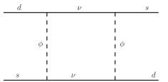
Figure 1: New contribution to $K-\bar{K}$ mixing induced by the scalar leptoquark $(\phi)$.

The new effects modify the observables $C_{\Delta m_{K}}$ and $C_{\varepsilon_{K}}$, and in the approximation $M_{\phi}^{2}\gg m^{2}_{t,W}$, their expressions are given by

$$C_{\Delta m_{K}} = 1+\frac{1}{g_{2}^{4}}\frac{M_{W}^{2}}{M_{\phi}^{2}}\frac{\eta_{tt}}{{\rm Re}(F^{*})}{\rm Re}\left(\xi_{ds}\right)^{2},$$ (10)

$$C_{\varepsilon_{K}} = 1+\frac{1}{g_{2}^{4}}\frac{M_{W}^{2}}{M_{\phi}^{2}}\frac{\eta_{tt}}{{\rm Im}(F^{*})}{\rm Im}\left(\xi_{ds}\right)^{2},$$ (11)

where we have used notation $F$ for $F(\lambda_{c},\lambda_{t},x_{c},x_{t})$ for simplicity. $g_{2}$ is the SU(2) gauge coupling and we define

$$\xi_{ds}\equiv(\lambda^{L}\lambda^{L\dagger})_{ds}=\sum_{i}\lambda^{L}_{d\nu_{i}}\lambda^{L\ast}_{s\nu_{i}}.$$ (12)

Solving Eqs. (10) and (11) for real and imaginary parts of $\xi_{ds}$ in terms of the experimental observables $C_{\Delta m_{K}}$ and $C_{\varepsilon_{K}}$, we obtain the following expressions:

$$\left({\rm Re}\,\xi_{ds}\right)^{2} = \left(\frac{g_{2}^{4}}{2}\frac{M_{\phi}^{2}}{M_{W}^{2}}\right)\Biggl{(}\frac{{\rm Re}(F^{*})}{\eta_{tt}}\Bigl{(}-1+C_{\Delta m_{K}}\Bigr{)}\Biggr{)}$$

$$\times\Biggl{(}1+\sqrt{1+\left(\frac{{\rm Im}F^{*}}{{\rm Re}F^{*}}\cdot\frac{C_{\varepsilon_{K}}-1}{C_{\Delta m_{K}}-1}\right)^{2}}\,\,\Biggr{)},$$

$$\left({\rm Im}\,\xi_{ds}\right)^{2} = \left(\frac{g_{2}^{4}}{2}\frac{M_{\phi}^{2}}{M_{W}^{2}}\right)\Biggl{(}\frac{{\rm Re}(F^{*})}{\eta_{tt}}\Bigl{(}-1+C_{\Delta m_{K}}\Bigr{)}\Biggr{)}$$

$$\times\Biggl{(}-1+\sqrt{1+\left(\frac{{\rm Im}F^{*}}{{\rm Re}F^{*}}\cdot\frac{C_{\varepsilon_{K}}-1}{C_{\Delta m_{K}}-1}\right)^{2}}\,\,\Biggr{)}.$$

To constrain the leptoquark couplings $\rm{Re}\,\xi_{ds}$ and $\rm{Im}\,\xi_{ds}$, we use the latest global fit results provided by the UTfit collaboration, and to be conservative evaluate the constraints at the 2$\sigma$ level: $C_{\Delta m_{K}}=1.10\pm 0.44$ and $C_{\varepsilon_{K}}=1.05\pm 0.32$ Bona:2007vi . Here, to account for the significant uncertainties from poorly known long-distance effects Buras:2014maa , we allow for a $\pm 40\%$ uncertainty in the case of $\Delta M_{K}$. For ${\rm Re}\,\xi_{ds}$ and ${\rm Im}\,\xi_{ds}$, we obtain the following upper bounds:

$$\left({\rm Re}\,\xi_{ds}\right)^{2}\leq 6.0\times 10^{-4}\left(\frac{M_{\phi}}{1000{\rm\,Ge\kern-1.25ptV}}\right)^{2},$$ (15)

$$\left({\rm Im}\,\xi_{ds}\right)^{2}\leq 3.8\times 10^{-4}\left(\frac{M_{\phi}}{1000{\rm\,Ge\kern-1.25ptV}}\right)^{2}.$$ (16)

As discussed in the next section, we find that a more constraining bound on the product of the couplings ${\rm Re}(\xi_{ds})$ and ${\rm Im}(\xi_{ds})$ can be obtained from theoretically rather clean rare processes $K^{+}\rightarrow\pi^{+}\nu\bar{\nu}$ and $K_{L}\rightarrow\pi^{0}\nu\bar{\nu}$ as compared to $K-\bar{K}$ mixing.

III Constraints from rare decay $K^{+}\rightarrow\pi^{+}\nu\bar{\nu}$

The charged and neutral $K\rightarrow\pi\nu\bar{\nu}$ are in many ways interesting FCNC processes and considered as golden modes. Both the decays can play an important role in indirect searches for NP because these decays are theoretically very clean and their branching ratio can be computed with an exceptionally high level of precision (for a review, see Ref. Buras:2004uu ). In the SM, these decays are dominated by Z-penguin and box diagrams, which exhibit hard, powerlike GIM suppression as compared to logarithmic GIM suppression generally seen in other loop-induced meson decays. At the leading order, both modes are induced by a single dimension-six local operator $(\bar{s}d)_{\rm V-A}(\bar{\nu}\nu)_{\rm V-A}$. The hadronic matrix element of this operator can be measured precisely in $K^{+}\rightarrow\pi^{0}e^{+}\nu$ decays, including isospin breaking corrections Mescia:2007kn ; Isidori:2005xm . The principal contribution to the error in theoretical predictions originates from the uncertainties on the current values of $\lambda_{t}$ and $m_{c}$. The long-distance effects are rather suppressed and have been found to be small Buchalla:1998ux ; Geng:1996kd ; Buchalla:1997kz .

In the SM, the effective Hamiltonian for $K\rightarrow\pi\nu\bar{\nu}$ decays is written as Buchalla:1993wq

$${\cal H}_{\rm eff}^{\rm SM} = \frac{G_{F}}{\sqrt{2}}\frac{2\alpha}{\pi\sin^{2}\theta_{W}}\sum_{\ell=e,\mu,\tau}\left(\lambda_{c}X_{\rm NNL}^{\ell}+\lambda_{t}X(x_{t})\right)$$ (17)

$$\hskip 56.9055pt\times(\bar{s}_{L}\gamma_{\mu}d_{L})(\bar{\nu}_{\ell L}\gamma^{\mu}\nu_{\ell L}),$$

The index $\ell=e,\mu,\tau$ denotes the lepton flavor. The short-distance function $X(x_{t})$ corresponds to the loop-function containing top contribution and is given by

$$X(x_{t})=\eta_{X}\cdot\frac{x_{t}}{8}\left[\frac{x_{t}+2}{x_{t}-1}+\frac{3x_{t}-6}{(x_{t}-1)^{2}}{\rm Ln}\,x_{t}\right],$$ (18)

where the factor $\eta_{X}$ includes the NLO correction and is close to unity ($\eta_{X}=0.995$), while the remaining part describes the contribution of top quark without QCD correction. The NLO QCD corrections have been computed in Refs. Buchalla:1993bv ; Misiak:1999yg ; Buchalla:1998ba , while two-loop electroweak corrections have been studied in Ref. Brod:2010hi . The loop-function $X_{\rm NNL}$ summarizes the contribution from the charm quark and can be written as Buras:1997ij

$$X_{NNL}=\frac{2}{3}X_{NNL}^{e}+\frac{1}{3}X_{NNL}^{\tau}\equiv\lambda^{4}P_{c}^{SD}(X),$$ (19)

where $\lambda=|V_{us}|$. The NLO results for the function $X_{\rm NNL}$ can be found in Refs. Buchalla:1998ba ; Buchalla:1993wq , while NNLO calculations are done in Refs. Buras:2005gr ; Buras:2006gb .

In the considered model, leptoquark $\phi$ mediates $K^{+}\rightarrow\pi^{+}\nu\bar{\nu}$ at tree level. The corresponding Feynman diagram is shown in Fig 2. Integrating out the heavy degrees of freedom, we obtain the following NP effective Hamiltonian relevant for $K^{+}\rightarrow\pi^{+}\nu\bar{\nu}$ decay:

 

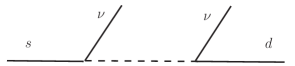
Figure 2: Feynman diagrams for the decay $K\rightarrow\pi\nu\bar{\nu}$ induced by the exchange of scalar leptoquark $\phi$.

$${\cal H}_{\rm eff}^{\rm NP}=-\frac{\lambda^{L\ast}_{s\nu_{\ell}}\lambda^{L}_{d\nu_{\ell}}}{2M_{\phi}^{2}}(\bar{s}\gamma_{\mu}Ld)(\bar{s}\gamma^{\mu}Ld).$$ (20)

The new contribution alters the SM branching ratio of $K^{+}\rightarrow\pi^{+}\nu\bar{\nu}$ Buras:2015qea as

$${\rm BR}(K^{+}\rightarrow\pi^{+}\nu\bar{\nu}) = \kappa_{+}(1+\Delta_{\rm EM})\left[\left(\frac{{\rm Im}\,\lambda_{t}}{\lambda^{5}}X_{\rm new}\right)^{2}\right.$$

$$+\left.\left(\frac{{\rm Re}\,\lambda_{c}}{\lambda}P_{c}(X)+\frac{{\rm Re}\,\lambda_{t}}{\lambda^{5}}X_{\rm new}\right)^{2}\right],$$

where $\kappa_{+}$ contains relevant hadronic matrix elements extracted from the decay rate of $K^{+}\rightarrow\pi^{0}e^{+}\nu$ along with isospin-breaking correction factor. The explicit form of $\kappa_{+}$ can be found in Ref. Buras:1998raa . $\Delta_{\rm EM}$ describes the electromagnetic radiative correction from photon exchanges and amounts to -0.3%. The charm contribution $P_{c}(X)$ includes the short-distance part $P_{c}^{\rm SD}(X)$ plus the long-distance contribution $\delta P_{c}$ (calculated in Ref. Isidori:2005xm ). We use $P_{c}(X)=0.404$ given in Ref. Buras:2015qea . The function $X_{\rm new}$ contains a new short-distance contribution from the leptoquark-mediated diagram and modifies the SM contribution through

​​

Figure 3: The constraints on ${\rm Re}(\xi_{ds})-{\rm Im}(\xi_{ds})$ parameter space from the measured value of ${\rm BR}(K^{+}\rightarrow\pi^{+}\nu\bar{\nu})$. The blue colored region shows experimentally allowed values at the $1\sigma$ level.

$$X_{new}=X(x_{t})+\frac{X_{\phi}}{\lambda_{t}},$$ (22)

where $X(x_{t})$ is the top contribution in the SM already defined in Eq. (18) and $X_{\phi}$ is the contribution due to leptoquark exchange. In terms of the model parameters, $X_{\phi}$ is given by

$$X_{\phi}=-\frac{\sqrt{2}}{4G_{F}}\frac{\pi\sin^{2}\theta_{W}}{\alpha}\frac{\xi_{ds}}{M_{\phi}^{2}},$$ (23)

where $\alpha(M_{Z})=1/127.9$ is the electromagnetic coupling constant, and $\sin^{2}\theta_{W}=0.23$ is the weak mixing angle. Using the experimental value of the branching ratio from the Particle Data Group, ${\rm BR}(K^{+}\rightarrow\pi^{+}\nu\bar{\nu})=(1.7\pm 1.1)\times 10^{-10}$ Agashe:2014kda , we obtain the constraint on ${\rm Re}\,\xi_{ds}$ and ${\rm Im}\,\xi_{ds}$, shown in Fig 3. A most conservative bound on individual couplings ${\rm Re}\,\xi_{ds}$ and ${\rm Im}\,\xi_{ds}$ can be obtained by taking only one set to be nonzero at a time. We find that for a leptoquark of $1{\rm\,Te\kern-1.25ptV}$ mass the constraints are given by $-7.2\times 10^{-4}<{\rm Re}\,\xi_{ds}<2.2\times 10^{-4}$ and $-3.3\times 10^{-4}<{\rm Im}\,\xi_{ds}<4.9\times 10^{-4}$. As pointed out before, these bounds rule out a large parameter space allowed from $K^{0}-\bar{K}^{0}$ mixing. The coupling ${\rm Im}\,\xi_{ds}$ can also be probed independently through the decay $K_{L}\rightarrow\pi^{0}\nu\bar{\nu}$, which is the subject of our next section.

IV Constraints from $K_{L}\rightarrow\pi^{0}\nu\bar{\nu}$

The neutral decay mode $K_{L}\rightarrow\pi^{0}\nu\bar{\nu}$ is CP-violating. In contrast to the decay rate of $K^{+}\rightarrow\pi^{+}\nu\bar{\nu}$ which depends on the real and imaginary parts of $\lambda_{t}$, with a small contribution from the real part of $\lambda_{c}$, the rate of $K_{L}\rightarrow\pi^{0}\nu\bar{\nu}$ depends only on Im$\lambda_{t}$. Because of the absence of the charm contribution, the prediction for ${\rm BR}(K_{L}\rightarrow\pi^{0}\nu\bar{\nu})$ is theoretically cleaner. The principal sources of error are the uncertainties on Im$\lambda_{t}$ and $m_{t}$. In the SM, the branching ratio is given by Buras:2004uu

$${\rm BR}(K_{L}\rightarrow\pi\nu\bar{\nu}) = \kappa_{L}\left(\frac{{\rm Im}\lambda_{t}}{\lambda^{5}}X(x_{t})\right)^{2},$$ (24)

with Buras:2015qea

$$\kappa_{L}=2.231\times 10^{-10}\left(\frac{\lambda}{0.225}\right)^{8}.$$ (25)

The exchange of leptoquark $\phi$ induces new contribution to the rate which can be accommodated in the expression of branching ratio by replacing $X(x_{t})$ with $X_{\rm new}$ given in Eq. (22). Experimentally, only a upper bound on the branching ratio is available: ${\rm BR}(K_{L}\rightarrow\pi^{0}\nu\bar{\nu})<2.8\times 10^{-8}$ at 90% C.L. Agashe:2014kda . In Fig 4, we plot the dependence of $K_{L}\rightarrow\pi\nu\bar{\nu}$ branching ratio on the imaginary part of the effective couplings $\xi_{ds}$. Numerically, the constraints are given by

​​

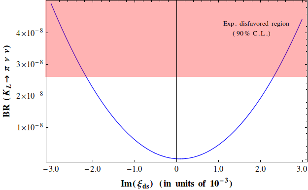
Figure 4: The dependence of ${\rm BR}(K_{L}\rightarrow\pi^{0}\nu\bar{\nu})$ on ${\rm Im}\,\xi_{ds}$. The red shaded region is currently disfavored by the experimental data at 90% C.L.

$$-0.0021<\frac{{\rm Im}\,\xi_{ds}}{\left(\frac{M_{\phi}}{1000{\rm\,Ge\kern-0.875ptV}}\right)^{2}}<0.0023,$$ (26)

Since the decay has not been observed so far and the present experimental limits are 3 orders of magnitude above the SM predictions Buras:2015qea , we find that constraints from $K_{L}\rightarrow\pi^{0}\nu\bar{\nu}$ are weaker compared to those obtained in the case of $K^{+}\rightarrow\pi^{+}\nu\bar{\nu}$.

V Constraints from $K_{L}\rightarrow\mu^{+}\mu^{-}$

The decay $K_{L}\rightarrow\mu^{+}\mu^{-}$ is sensitive to much of the same short-distance physics (i.e., $\lambda_{t}$ and $m_{t}$) as $K\rightarrow\pi\nu\bar{\nu}$ and therefore provides complementary information on the structure of FCNC $\lvert\Delta S\rvert=1$ transitions. This is important because experimentally a much more precise measurement compared to $K\rightarrow\pi\nu\bar{\nu}$ is available: ${\rm BR}(K_{L}\rightarrow\mu\mu)=(6.84\pm 0.11)\times 10^{-9}$ Agashe:2014kda . However, the theoretical situation is far more complex (for a review, see Refs. Ritchie:1993ua ; Cirigliano:2011ny ). The amplitude for $K_{L}\rightarrow\mu^{+}\mu^{-}$ can be decomposed into a dispersive (real) and an absorptive (imaginary) part. The dominant contribution to the absorptive part (as well as to total decay rate ($K_{L}\rightarrow\mu^{+}\mu^{-}$)) comes from the real two-photon intermediate state. The dispersive amplitude is the sum of the so-called long-distance and the short-distance contributions. Only the short-distance (SD) part can be reliably calculated. The most recent estimates of the SD part from data give ${\rm BR}(K_{L}\rightarrow\mu^{+}\mu^{-})_{\rm SD}\leq 2.5\times 10^{-9}$ Isidori:2003ts . The effective Hamiltonian relevant for the decay $K_{L}\rightarrow\mu^{+}\mu^{-}$ is given by Buchalla:1993wq

$${\cal H}_{\rm eff}(K_{L}\rightarrow\mu^{+}\mu^{-}) = \frac{G_{F}}{\sqrt{2}}\frac{\alpha}{2\pi\sin^{2}\!\theta_{W}}(\lambda_{c}Y_{NL}+\lambda_{t}Y(x_{t}))$$

$$\hskip 22.76228pt\times(\bar{s}\gamma^{\mu}(1-\gamma_{5})d)(\bar{\mu}\gamma_{\mu}\gamma_{5}\mu),$$

$$= \frac{G_{F}}{\sqrt{2}}V^{*}_{us}V_{ud}\,\,\Delta^{K}_{SM}$$

$$\hskip 14.22636pt\times(\bar{s}\gamma^{\mu}(1-\gamma_{5})d)(\bar{\mu}\gamma_{\mu}\gamma_{5}\mu),$$

where $\Delta^{K}_{SM}$ describes the Wilson coefficient (WC) of the effective local operator $(\bar{s}d)_{\rm V-A}(\bar{\mu}\gamma_{\mu}\gamma_{5}\mu)$ and is given as

$$\Delta^{K}_{SM}=\frac{\alpha(\lambda_{c}Y_{NL}+\lambda_{t}Y(x_{t}))}{2\pi\sin^{2}\!\theta_{w}\,V^{*}_{us}V_{ud}}.$$ (28)

The short-distance function $Y(x_{t})$ describes contribution from Z-penguin and box diagrams with an internal top quark with QCD corrections. Its expression in NLO can be written as Misiak:1999yg ; Buchalla:1998ba

$$Y(x_{t})=\eta_{Y}\cdot\frac{x_{t}}{8}\left(\frac{4-x_{t}}{1-x_{t}}+\frac{3x_{t}}{(1-x_{t})^{2}}{\rm Ln}\,x_{t}\right),$$ (29)

where the factor $\eta_{Y}$ summarizes the QCD corrections ($\eta_{Y}=1.012$). The function $Y_{\rm NL}$ represents the contribution of loop-diagrams involving internal charm-quark exchange and is known to NLO Buchalla:1993wq ; Buchalla:1998ba and recently to NNLO Gorbahn:2006bm . The charm contribution is also often denoted by $P_{c}(Y)$ and is related to $Y_{NL}$ analogous to the relation in Eq (19). In the SM, the branching ratio for the SD part is written as Crivellin:2016vjc ; Gorbahn:2006bm

$${\rm BR}(K_{L}\rightarrow\mu^{+}\mu^{-})_{SM}({\rm SD}) = \frac{N_{K}^{2}}{2\pi\,\Gamma_{K_{L}}}\left(\frac{m_{\mu}}{m_{K}}\right)^{2}\sqrt{1-\frac{4\,m_{\mu}^{2}}{m_{K}^{2}}}$$

$$\hskip 19.91684pt\times\,\,f_{K}^{2}m_{K}^{3}({\rm Re}\,\Delta^{K}_{SM})^{2},$$

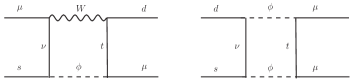
Figure 5: Feynman diagrams relevant for the decay $K_{L}\rightarrow\mu^{+}\mu^{-}$ induced by the scalar leptoquark $\phi$.

where $N_{K}=G_{F}V_{us}^{\ast}V_{ud}$ and $\Gamma_{K_{L}}$ is the decay width of $K_{L}$. Before proceeding to discuss the constraints on leptoquark couplings from $K_{L}\rightarrow\mu^{+}\mu^{-}$, we give a description of the “operator basis” we use in the present and next sections. The effective Hamiltonian for $K_{L}\rightarrow\mu^{+}\mu^{-}$ in Eq. (V) is written in the operator basis of {$Q_{7V},\,Q_{7A}$} following Ref. Crivellin:2016vjc . In what follows, we will switch to the {$Q^{K}_{VLL},\,Q^{K}_{VLR}$} operator basis. The operators in both bases are written as

$$Q_{7V} = (\bar{s}\gamma_{\alpha}(1-\gamma_{5})d)(\bar{\mu}\gamma^{\alpha}\mu),$$

$$Q_{7A} = (\bar{s}\gamma_{\alpha}(1-\gamma_{5})d)(\bar{\mu}\gamma^{\alpha}\gamma_{5}\mu),$$ (31)

and

$$Q^{K}_{VLL} = (\bar{s}\gamma_{\alpha}Ld)(\bar{\mu}\gamma^{\alpha}L\mu),$$

$$Q^{K}_{VLR} = (\bar{s}\gamma_{\alpha}Ld)(\bar{\mu}\gamma^{\alpha}R\mu).$$ (32)

To change from the basis {$Q_{7V},\,Q_{7A}$} to the basis {$Q^{K}_{VLL},\,Q^{K}_{VLR}$}, the following transformation rules hold:

$$Q^{K}_{VLL}=\frac{1}{4}\left(Q_{7V}-Q_{7A}\right),\hskip 14.22636ptQ^{K}_{VLR}=\frac{1}{4}\left(Q_{7V}+Q_{7A}\right).$$

The scalar leptoquark $\phi$ contributes to the quark-level transition $\bar{s}\rightarrow\bar{d}\mu^{+}\mu^{-}$ at the leading order through loop diagrams. The Feynman diagrams relevant for $K_{L}\rightarrow\mu^{+}\mu^{-}$ are shown in Fig 5. These diagrams are similar to the ones calculated in the case of $b\rightarrow s\mu\mu$ in Ref. Bauer:2015knc . Correcting for the different quark content and coupling, and taking into account the prefactors in the definitions of the effective Hamiltonian for K and B system, we can straightforwardly obtain the result for NP Wilson coefficients of effective operators $Q^{K}_{VLL}$, $Q^{K}_{VLR}$ and are given by

$$C_{VLL}^{K(new)} = -\frac{1}{8\pi^{2}}\frac{\lambda_{t}}{\lambda_{u}}\frac{m_{t}^{2}}{M_{\phi}^{2}}\lvert\lambda_{t\mu}^{L}\rvert^{2}$$ (34)

$$+\,\,\frac{\sqrt{2}}{64G_{F}\pi^{2}M_{\phi}^{2}}\frac{\xi_{ds}\,\xi^{L}_{\mu\mu}}{\lambda_{u}},$$

$$C_{VLR}^{K(new)} = -\frac{1}{16\pi^{2}}\frac{\lambda_{t}}{\lambda_{u}}\frac{m_{t}^{2}}{M_{\phi}^{2}}\lvert\lambda_{t\mu}^{R}\rvert^{2}\left({\rm Ln}\frac{M_{\phi}^{2}}{m_{t}^{2}}-f(x_{t})\right)$$ (35)

$$+\,\,\frac{\sqrt{2}}{64G_{F}\pi^{2}M_{\phi}^{2}}\frac{\xi_{ds}\,\xi^{R}_{\mu\mu}}{\lambda_{u}},$$

where the function $f(x_{t})$ depends on the top-quark mass and is given in Ref. Bauer:2015knc and we define

$$\xi^{L(R)}_{\ell\ell^{{}^{\prime}}}=\sum_{i}\lambda^{L(R)\ast}_{u_{i}\ell}\lambda^{L(R)}_{u_{i}\ell^{{}^{\prime}}}.$$ (36)

​​

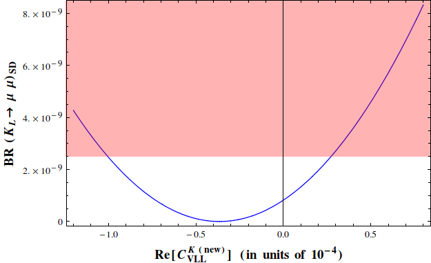
Figure 6: The dependence of ${\rm BR}(K_{L}\rightarrow\mu^{+}\mu^{-})$ on the Wilson coefficient $C_{VLL}^{K(new)}$. We have assumed one-operator dominance as discussed in the text. The red shaded region shows the experimentally disallowed values at $1\sigma$.

The one advantage we get by the change of basis is that the contribution of right-handed interaction terms in the Lagrangian (Eq. (I)) is contained only in $C_{VLR}^{K(new)}$. After accommodating the leptoquark contribution to the SM value, the total SD branching ratio for the decay $K_{L}\rightarrow\mu^{+}\mu^{-}$ is given by

$${\rm BR}(K_{L}\rightarrow\mu^{+}\mu^{-})_{\rm SD} = \frac{N_{K}^{2}}{2\pi\,\Gamma_{K_{L}}}\left(\frac{m_{\mu}}{m_{K}}\right)^{2}\sqrt{1-\frac{4\,m_{\mu}^{2}}{m_{K}^{2}}}$$

$$\times f_{K}^{2}m_{K}^{3}\lambda^{10}\left\{\frac{{\rm Re}\lambda_{c}}{\lambda}\frac{\alpha\,P_{c}(Y)}{2\pi\sin^{2}\!\theta_{W}\lambda_{u}}\right.$$

$$+\frac{1}{\lambda^{5}}\left.\left({\rm Re}\lambda_{t}\frac{\alpha\,Y(x_{t})}{2\pi\sin^{2}\!\theta_{W}\lambda_{u}}\right.\right.$$

$$\left.\left.+\frac{1}{4}{\rm Re}(C_{VLR}^{K(new)}-C_{VLL}^{K(new)})\right)\right\}^{2},$$

To simplify further the analysis, we invoke the assumption that except the SM contribution only one of the NP operators contributes dominantly. This assumption helps us in determining the limits on the dominant WC from ${\rm BR}\,(K_{L}\rightarrow\mu^{+}\mu^{-})_{\rm SD}$, and the generalization of this situation to incorporate more than one NP operator contribution is straight forward. Therefore, in what follows, we will ignore the contribution of the right-handed operator in further analysis. In Fig 6, we show the dependence of the SD part of BR($K_{L}\rightarrow\mu^{+}\mu^{-}$) on ${\rm Re}\,C_{VLL}^{K(new)}$. Numerically the bound on the WC reads $-1.00\times 10^{-4}<{\rm Re}\,C_{VLL}^{K(new)}<0.27\times 10^{-4}$. We use the upper bound to constrain the generation-diagonal leptoquark couplings in the following way. Employing Eq. (34), the upper bound on the WC can be written in terms of model parameters as

$$\left(-\frac{1}{8\pi^{2}}\frac{\rm{Re}\,\lambda_{t}}{\lambda_{u}}\frac{m_{t}^{2}}{M_{\phi}^{2}}\lvert\lambda_{t\mu}^{L}\rvert^{2}+\frac{\sqrt{2}}{64G_{F}\pi^{2}M_{\phi}^{2}}\frac{\rm{Re}\,\xi_{ds}}{\lambda_{u}}\,\xi^{L}_{\mu\mu}\right)$$

$$<0.27\times 10^{-4},$$ (38)

Assuming the worst possible case in which the bound on $\rm{Re}\,\xi_{ds}$ from $K^{+}\rightarrow\pi^{+}\nu\bar{\nu}$ (as obtained in section III) is saturated, i.e., using $\rm{Re}\,\xi_{ds}=2.2\times 10^{-4}$ in the above equation, we get

$$\sqrt{\lvert\lambda_{u\mu}^{L}\rvert^{2}+\lvert\lambda_{c\mu}^{L}\rvert^{2}+\left(1+\frac{2.52}{(\frac{M_{\phi}}{1000{\rm\,Ge\kern-0.875ptV}})^{2}}\right)\lvert\lambda_{t\mu}^{L}\rvert^{2}}<11.83.$$

We find that constraints from the SD branching ratio of $K_{L}\rightarrow\mu^{+}\mu^{-}$ are not severe and large $\sim O(1)$ generation-diagonal leptoquark couplings are allowed. To this end, we must mention that the above bound is in agreement with the constraint obtained in Ref. Bauer:2015knc (see Eq.(17) therein) while explaining the anomaly in $R_{K}$ in this model. We also note from Eq. (V) that the top contribution to $\bar{s}\rightarrow\bar{d}\mu^{+}\mu^{-}$ for the considered masses of the leptoquark $(\sim 1{\rm\,Te\kern-1.25ptV})$ is largely enhanced in contrast to the effects found in the case of $b\rightarrow s\mu^{+}\mu^{-}$ processes Bauer:2015knc where the top contribution is suppressed for the same choice of the leptoquark masses.

VI Constraints from LFV decay $K_{L}\rightarrow\mu^{\mp}{e}^{\pm}$

In this section, we discuss the effects of the leptoquark $\phi$ on LFV process $K\rightarrow\mu^{\mp}e^{\pm}$. Experimentally, there is only an upper bound on this process: BR$(K_{L}\rightarrow\mu^{\mp}e^{\pm})<4.7\times 10^{-12}$ Agashe:2014kda . LFV processes are interesting because in the SM they are forbidden. Therefore, any observation of such process immediately indicates towards the presence of NP. The leptoquark $\phi$ can mediate $K_{L}\rightarrow\mu e$ decay through similar diagrams shown in Fig 5 with one of the $\mu$ lines being replaced with $e$. After integrating out heavy particles, new effective operators relevant for $K_{L}\rightarrow\mu e$ are generated. The operators are similar to those in Eq. (V) but with one of the $\mu$ changed to $e$. The branching ratio in terms of the new Wilson coefficients $C_{VLL}^{\mu e}$ and $C_{VLR}^{\mu e}$ is given by Crivellin:2016vjc

$${\rm BR}(K_{L}\rightarrow\mu e) = \frac{N_{K}^{2}f_{K}^{2}}{64\pi\Gamma_{K_{L}}}\left(\frac{m_{\mu}}{m_{K}}\right)^{2}\left(1-\frac{m_{\mu}^{2}}{m_{K}^{2}}\right)^{2}$$ (40)

$$\times\left(\lvert C_{VLL}^{\mu e}\rvert^{2}+\lvert C_{VLR}^{\mu e}\rvert^{2}\right),$$

Adapting the results of Eq. (34) to the LFV case, we find

$$C_{VLL}^{\mu e} = -\frac{1}{8\pi^{2}}\frac{\lambda_{t}}{\lambda_{u}}\frac{m_{t}^{2}}{M_{\phi}^{2}}(\lambda^{L}_{te}\lambda^{L\ast}_{t\mu})$$ (41)

$$+\,\,\frac{\sqrt{2}}{64G_{F}\pi^{2}M_{\phi}^{2}}\frac{\xi_{ds}\,\xi^{L}_{\mu e}}{\lambda_{u}},$$

$$C_{VLR}^{\mu e} = -\frac{1}{16\pi^{2}}\frac{\lambda_{t}}{\lambda_{u}}\frac{m_{t}^{2}}{M_{\phi}^{2}}(\lambda^{R}_{t\mu}\lambda^{R}_{te})\left({\rm Ln}\frac{M_{\phi}^{2}}{m_{t}^{2}}-f(x_{t})\right)$$ (42)

$$+\,\,\frac{\sqrt{2}}{64G_{F}\pi^{2}M_{\phi}^{2}}\frac{\xi_{ds}\,\xi^{R}_{\mu e}}{\lambda_{u}}.$$

Using the current experimental bound on $K_{L}\rightarrow\mu e$, we get $\left[\lvert C_{VLL}^{\mu e}\rvert^{2}+\lvert C_{VLR}^{\mu e}\rvert^{2}\right]^{1/2}<3.9\times 10^{-6}$. Following the similar analysis as done in section V for the case of $K_{L}\rightarrow\mu\mu$, we obtain the constraints on the leptoquark couplings,

$$\Biggl{(}\sqrt{(\lambda_{u\mu}^{L}\lambda_{ue}^{L})+(\lambda_{c\mu}^{L}\lambda_{ce}^{L})+\left(1+\frac{2.52}{(\frac{M_{\phi}}{1000{\rm\,Ge\kern-0.875ptV}})^{2}}\right)(\lambda_{t\mu}^{L}\lambda_{te}^{L})}\Biggr{)}$$

$$<4.49,$$

where the top contribution is again enhanced. For simplicity we assumed the couplings to be real. Here, we would like to mention that the same Wilson coefficients also contribute to other LFV processes such as $K\rightarrow\pi\mu e$. However, as pointed out in Ref. Crivellin:2016vjc , the constraints on Wilson coefficients $\left(\lvert C_{VLL}^{\mu e}\rvert^{2}+\lvert C_{VLR}^{\mu e}\rvert^{2}\right)^{1/2}$ are about an order of magnitude weaker than the one from $K_{L}\rightarrow\mu^{\mp}e^{\pm}$. Therefore, experimental data on $K\rightarrow\pi\mu e$ do not improve the constraints obtained in Eq. (VI).

VII Results and Discussion

In light of several anomalies observed in semileptonic B decays, often explained by invoking leptoquark NP models, we have studied a scalar leptoquark model in the context of rare decays of kaons and neutral kaon mixing. The model is interesting because it can provide one of the possible explanations for the observed discrepancies in semileptonic B decays. We examined the effects of leptoquark contribution to the several kaon processes involving $K^{0}-\bar{K^{0}}$ mixing, $K^{+}\rightarrow\pi^{+}\nu\bar{\nu}$, $K_{L}\rightarrow\pi^{0}\nu\bar{\nu}$, $K_{L}\rightarrow\mu^{+}\mu^{-}$, and LFV decay $K_{L}\rightarrow\mu^{\mp}e^{\pm}$. Working in the framework of EFT, we have discussed the effective operators generated after integrating out heavy particles and written down the explicit expressions of the corresponding Wilson coefficient in terms of the leptoquark couplings. Using the present experimental information on these decays, we derived bounds on the couplings relevant for kaon processes. We found that the constraints from $K^{0}-\bar{K^{0}}$ on the real and imaginary parts of left-handed coupling $\xi_{ds}$ are $\sim O(10^{-2})$. However, the same set of couplings can also be constrained from ${\rm BR}(K^{+}\rightarrow\pi^{+}\nu\bar{\nu})$, ${\rm BR}(K_{L}\rightarrow\pi^{0}\nu\bar{\nu})$, and it was found that constraints from the rare process ${\rm BR}(K^{+}\rightarrow\pi^{+}\nu\bar{\nu})$ are about 2 orders of magnitude more severe than those obtained from the mixing of neutral kaons. In fact, the decay ${\rm BR}(K^{+}\rightarrow\pi^{+}\nu\bar{\nu})$ gives the most stringent constraints on the leptoquark couplings among all the processes studied in this work and therefore is the most interesting observable to test the NP effects of the scalar leptoquark in the kaon sector. Assuming a one-operator dominance scenario, we constrained the NP Wilson coefficient contributing to the rate of $K_{L}\rightarrow\mu^{+}\mu^{-}$. We further used the bounds on the NP Wilson coefficient to obtain the constraints on generation-diagonal leptoquark couplings. We found that the present measured value of ${\rm BR}(K_{L}\rightarrow\mu^{+}\mu^{-})$ allows generation-diagonal coupling of the leptoquark to be $\sim O(1)$. The constraint on the combination of generation-diagonal couplings from $K_{L}\rightarrow\mu^{+}\mu^{-}$ is in agreement with the one obtained in Ref. Bauer:2015knc for explaining experimental data on $R_{K}$. However, whereas the top contribution to $b\rightarrow s\mu^{+}\mu^{-}$ is suppressed, we found that in the case of $\bar{s}\rightarrow\bar{d}\mu^{+}\mu^{-}$ the top contribution is enhanced for the considered range of leptoquark masses. We also did a similar analysis for the case of LFV decay $K_{L}\rightarrow\mu^{\mp}e^{\pm}$, which involves generation-diagonal as well as off-diagonal couplings. We found that present experimental limits on ${\rm BR}\,(K_{L}\rightarrow\mu^{\mp}e^{\pm})$ do not provide very strong constraints, and involved couplings can be as large as $\sim O(1)$.

Acknowledgements: The author would like to thank Namit Mahajan, Anjan Joshipura, and Saurabh Rindani for many helpful discussions. The author would like to thank Monika Blanke for a very useful communication regarding kaon mixing observables. The author also thanks Abhaya Swain and Chandan Hati for help with the preparation of this manuscript.

References

- (1) G. Aad et al. [ATLAS Collaboration], Phys. Lett. B 716, 1 (2012) doi:10.1016/j.physletb.2012.08.020 [arXiv:1207.7214 [hep-ex]].
- (2) S. Chatrchyan et al. [CMS Collaboration], Phys. Lett. B 716, 30 (2012) doi:10.1016/j.physletb.2012.08.021 [arXiv:1207.7235 [hep-ex]].
- (3) G. Ricciardi et al., Eur. Phys. J. Plus 130, no. 10, 209 (2015) doi:10.1140/epjp/i2015-15209-y [arXiv:1507.05029 [hep-ph]]; J. Ellis, arXiv:1604.00333 [hep-ph].
- (4) R. Aaij et al. [LHCb Collaboration], Phys. Rev. Lett. 115, no. 11, 111803 (2015) [arXiv:1506.08614 [hep-ex]].
- (5) J. P. Lees et al. [BaBar Collaboration], Phys. Rev. Lett. 109, 101802 (2012) [arXiv:1205.5442 [hep-ex]]; J. P. Lees et al. [BaBar Collaboration], Phys. Rev. D 88, no. 7, 072012 (2013) [arXiv:1303.0571 [hep-ex]].
- (6) M. Huschle et al. [Belle Collaboration], arXiv:1507.03233 [hep-ex].
- (7) S. Fajfer, J. F. Kamenik and I. Nisandzic, Phys. Rev. D 85, 094025 (2012) doi:10.1103/PhysRevD.85.094025 [arXiv:1203.2654 [hep-ph]]; H. Na et al. [HPQCD Collaboration], Phys. Rev. D 92, no. 5, 054510 (2015) [arXiv:1505.03925 [hep-lat]].
- (8) R. Aaij et al. [LHCb Collaboration], Phys. Rev. Lett. 113, 151601 (2014) doi:10.1103/PhysRevLett.113.151601 [arXiv:1406.6482 [hep-ex]].
- (9) C. Bobeth, G. Hiller and G. Piranishvili, JHEP 0712, 040 (2007) doi:10.1088/1126-6708/2007/12/040 [arXiv:0709.4174 [hep-ph]].
- (10) G. Hiller and F. Kruger, Phys. Rev. D 69, 074020 (2004) doi:10.1103/PhysRevD.69.074020 [hep-ph/0310219].
- (11) R. Aaij et al. [LHCb Collaboration], Phys. Rev. Lett. 111, 191801 (2013) doi:10.1103/PhysRevLett.111.191801 [arXiv:1308.1707 [hep-ex]].
- (12) R. Aaij et al. [LHCb Collaboration], JHEP 1602, 104 (2016) doi:10.1007/JHEP02(2016)104 [arXiv:1512.04442 [hep-ex]].
- (13) S. Descotes-Genon, J. Matias, M. Ramon and J. Virto, JHEP 1301, 048 (2013) doi:10.1007/JHEP01(2013)048 [arXiv:1207.2753 [hep-ph]].
- (14) J. Matias, F. Mescia, M. Ramon and J. Virto, JHEP 1204, 104 (2012) doi:10.1007/JHEP04(2012)104 [arXiv:1202.4266 [hep-ph]].
- (15) S. Descotes-Genon, T. Hurth, J. Matias and J. Virto, JHEP 1305, 137 (2013) doi:10.1007/JHEP05(2013)137 [arXiv:1303.5794 [hep-ph]].
- (16) R. Aaij et al. [LHCb Collaboration], JHEP 1509, 179 (2015) doi:10.1007/JHEP09(2015)179 [arXiv:1506.08777 [hep-ex]].
- (17) S. Descotes-Genon, J. Matias and J. Virto, Phys. Rev. D 88, 074002 (2013) doi:10.1103/PhysRevD.88.074002 [arXiv:1307.5683 [hep-ph]].
- (18) W. Altmannshofer and D. M. Straub, arXiv:1503.06199 [hep-ph].
- (19) S. Descotes-Genon, L. Hofer, J. Matias and J. Virto, JHEP 1606, 092 (2016) doi:10.1007/JHEP06(2016)092 [arXiv:1510.04239 [hep-ph]].
- (20) A. Celis, M. Jung, X. Q. Li and A. Pich, JHEP 1301, 054 (2013) [arXiv:1210.8443 [hep-ph]].
- (21) P. Ko, Y. Omura and C. Yu, JHEP 1303, 151 (2013) [arXiv:1212.4607 [hep-ph]].
- (22) A. Crivellin, C. Greub and A. Kokulu, Phys. Rev. D 86, 054014 (2012) [arXiv:1206.2634 [hep-ph]].
- (23) N. G. Deshpande and A. Menon, JHEP 1301, 025 (2013) [arXiv:1208.4134 [hep-ph]].
- (24) C. Hati, G. Kumar and N. Mahajan, JHEP 1601, 117 (2016) doi:10.1007/JHEP01(2016)117 [arXiv:1511.03290 [hep-ph]].
- (25) A. Datta, M. Duraisamy and D. Ghosh, Phys. Rev. D 86, 034027 (2012) [arXiv:1206.3760 [hep-ph]].
- (26) M. Tanaka and R. Watanabe, Phys. Rev. D 87, no. 3, 034028 (2013) [arXiv:1212.1878 [hep-ph]].
- (27) M. Freytsis, Z. Ligeti and J. T. Ruderman, Phys. Rev. D 92, no. 5, 054018 (2015) [arXiv:1506.08896 [hep-ph]].
- (28) S. Bhattacharya, S. Nandi and S. K. Patra, arXiv:1509.07259 [hep-ph].
- (29) I. Dorsner, S. Fajfer, J. F. Kamenik and N. Kosnik, Phys. Lett. B 682, 67 (2009) doi:10.1016/j.physletb.2009.10.087 [arXiv:0906.5585 [hep-ph]].
- (30) Y. Sakaki, M. Tanaka, A. Tayduganov and R. Watanabe, Phys. Rev. D 88, no. 9, 094012 (2013) [arXiv:1309.0301 [hep-ph]].
- (31) S. Fajfer, J. F. Kamenik, I. Nisandzic and J. Zupan, Phys. Rev. Lett. 109, 161801 (2012) [arXiv:1206.1872 [hep-ph]].
- (32) I. Doršner, S. Fajfer, N. Košnik and I. Nišandžić, JHEP 1311, 084 (2013) doi:10.1007/JHEP11(2013)084 [arXiv:1306.6493 [hep-ph]].
- (33) T. Blake, T. Gershon and G. Hiller, Ann. Rev. Nucl. Part. Sci. 65, 113 (2015) doi:10.1146/annurev-nucl-102014-022231 [arXiv:1501.03309 [hep-ex]].
- (34) R. Gauld, F. Goertz and U. Haisch, JHEP 1401, 069 (2014) doi:10.1007/JHEP01(2014)069 [arXiv:1310.1082 [hep-ph]].
- (35) S. L. Glashow, D. Guadagnoli and K. Lane, Phys. Rev. Lett. 114, 091801 (2015) doi:10.1103/PhysRevLett.114.091801 [arXiv:1411.0565 [hep-ph]].
- (36) A. Crivellin, G. D’Ambrosio and J. Heeck, Phys. Rev. D 91, no. 7, 075006 (2015) doi:10.1103/PhysRevD.91.075006 [arXiv:1503.03477 [hep-ph]].
- (37) W. Altmannshofer, S. Gori, M. Pospelov and I. Yavin, Phys. Rev. D 89, 095033 (2014) doi:10.1103/PhysRevD.89.095033 [arXiv:1403.1269 [hep-ph]].
- (38) A. J. Buras and J. Girrbach, JHEP 1312, 009 (2013) doi:10.1007/JHEP12(2013)009 [arXiv:1309.2466 [hep-ph]].
- (39) A. Crivellin, G. D’Ambrosio and J. Heeck, Phys. Rev. Lett. 114, 151801 (2015) doi:10.1103/PhysRevLett.114.151801 [arXiv:1501.00993 [hep-ph]].
- (40) C. W. Chiang, X. G. He and G. Valencia, arXiv:1601.07328 [hep-ph].
- (41) S. M. Boucenna, A. Celis, J. Fuentes-Martin, A. Vicente and J. Virto, Phys. Lett. B 760, 214 (2016) doi:10.1016/j.physletb.2016.06.067 [arXiv:1604.03088 [hep-ph]].
- (42) B. Gripaios, M. Nardecchia and S. A. Renner, JHEP 1505, 006 (2015) doi:10.1007/JHEP05(2015)006 [arXiv:1412.1791 [hep-ph]].
- (43) D. Bečirević, S. Fajfer and N. Košnik, Phys. Rev. D 92, no. 1, 014016 (2015) doi:10.1103/PhysRevD.92.014016 [arXiv:1503.09024 [hep-ph]].
- (44) R. Alonso, B. Grinstein and J. M. Camalich, JHEP 1510, 184 (2015) doi:10.1007/JHEP10(2015)184 [arXiv:1505.05164 [hep-ph]].
- (45) L. Calibbi, A. Crivellin and T. Ota, Phys. Rev. Lett. 115, 181801 (2015) doi:10.1103/PhysRevLett.115.181801 [arXiv:1506.02661 [hep-ph]].
- (46) M. Bauer and M. Neubert, Phys. Rev. Lett. 116, no. 14, 141802 (2016) doi:10.1103/PhysRevLett.116.141802 [arXiv:1511.01900 [hep-ph]].
- (47) G. Hiller and M. Schmaltz, Phys. Rev. D 90, 054014 (2014) doi:10.1103/PhysRevD.90.054014 [arXiv:1408.1627 [hep-ph]].
- (48) R. Barbieri, G. Isidori, A. Pattori and F. Senia, Eur. Phys. J. C 76, no. 2, 67 (2016) doi:10.1140/epjc/s10052-016-3905-3 [arXiv:1512.01560 [hep-ph]].
- (49) S. Fajfer and N. Košnik, Phys. Lett. B 755, 270 (2016) doi:10.1016/j.physletb.2016.02.018 [arXiv:1511.06024 [hep-ph]].
- (50) I. de Medeiros Varzielas and G. Hiller, JHEP 1506, 072 (2015) doi:10.1007/JHEP06(2015)072 [arXiv:1503.01084 [hep-ph]].
- (51) M. Blanke, PoS KAON 13, 010 (2013) [arXiv:1305.5671 [hep-ph]].
- (52) A. J. Buras and J. Girrbach, Acta Phys. Polon. B 43, 1427 (2012) doi:10.5506/APhysPolB.43.1427 [arXiv:1204.5064 [hep-ph]].
- (53) A. J. Buras, T. Ewerth, S. Jager and J. Rosiek, Nucl. Phys. B 714, 103 (2005) doi:10.1016/j.nuclphysb.2005.02.014 [hep-ph/0408142].
- (54) M. Blanke, A. J. Buras, B. Duling, S. Recksiegel and C. Tarantino, Acta Phys. Polon. B 41, 657 (2010) [arXiv:0906.5454 [hep-ph]].
- (55) M. Blanke, A. J. Buras, B. Duling, K. Gemmler and S. Gori, JHEP 0903, 108 (2009) doi:10.1088/1126-6708/2009/03/108 [arXiv:0812.3803 [hep-ph]].
- (56) M. Bauer, S. Casagrande, U. Haisch and M. Neubert, JHEP 1009, 017 (2010) doi:10.1007/JHEP09(2010)017 [arXiv:0912.1625 [hep-ph]].
- (57) C. J. Lee and J. Tandean, JHEP 1508, 123 (2015) doi:10.1007/JHEP08(2015)123 [arXiv:1505.04692 [hep-ph]].
- (58) A. J. Buras, F. De Fazio, J. Girrbach and M. V. Carlucci, JHEP 1302, 023 (2013) doi:10.1007/JHEP02(2013)023 [arXiv:1211.1237 [hep-ph]].
- (59) A. J. Buras, F. De Fazio and J. Girrbach-Noe, JHEP 1408, 039 (2014) doi:10.1007/JHEP08(2014)039 [arXiv:1405.3850 [hep-ph]].
- (60) A. J. Buras and J. Girrbach, Rept. Prog. Phys. 77, 086201 (2014) doi:10.1088/0034-4885/77/8/086201 [arXiv:1306.3775 [hep-ph]].
- (61) A. J. Buras, A. Romanino and L. Silvestrini, Nucl. Phys. B 520, 3 (1998) doi:10.1016/S0550-3213(98)00169-2 [hep-ph/9712398].
- (62) F. S. Queiroz, K. Sinha and A. Strumia, Phys. Rev. D 91, no. 3, 035006 (2015) doi:10.1103/PhysRevD.91.035006 [arXiv:1409.6301 [hep-ph]].
- (63) F. Mescia and J. Virto, Phys. Rev. D 86, 095004 (2012) doi:10.1103/PhysRevD.86.095004 [arXiv:1208.0534 [hep-ph]].
- (64) ATLAS and CMS physics results from Run-II, see: http://indico.cern.ch/event/442432/
- (65) S. Sahoo and R. Mohanta, Phys. Rev. D 91, no. 9, 094019 (2015) doi:10.1103/PhysRevD.91.094019 [arXiv:1501.05193 [hep-ph]].
- (66) S. Fajfer and N. Kosnik, Phys. Rev. D 79, 017502 (2009) doi:10.1103/PhysRevD.79.017502 [arXiv:0810.4858 [hep-ph]].
- (67) S. de Boer and G. Hiller, arXiv:1510.00311 [hep-ph].
- (68) S. Fajfer and N. Košnik, Eur. Phys. J. C 75, no. 12, 567 (2015) doi:10.1140/epjc/s10052-015-3801-2 [arXiv:1510.00965 [hep-ph]].
- (69) M. Antonelli et al., Phys. Rept. 494, 197 (2010) doi:10.1016/j.physrep.2010.05.003 [arXiv:0907.5386 [hep-ph]].
- (70) G. Buchalla, A. J. Buras and M. E. Lautenbacher, Rev. Mod. Phys. 68, 1125 (1996) doi:10.1103/RevModPhys.68.1125 [hep-ph/9512380].
- (71) T. Inami and C. S. Lim, Prog. Theor. Phys. 65, 297 (1981) [Prog. Theor. Phys. 65, 1772 (1981)]. doi:10.1143/PTP.65.297
- (72) G. C. Branco, L. Lavoura and J. P. Silva, Int. Ser. Monogr. Phys. 103, 1 (1999).
- (73) A. J. Buras, M. Jamin and P. H. Weisz, Nucl. Phys. B 347, 491 (1990). doi:10.1016/0550-3213(90)90373-L
- (74) J. Brod and M. Gorbahn, Phys. Rev. Lett. 108, 121801 (2012) doi:10.1103/PhysRevLett.108.121801 [arXiv:1108.2036 [hep-ph]].
- (75) J. Brod and M. Gorbahn, Phys. Rev. D 82, 094026 (2010) doi:10.1103/PhysRevD.82.094026 [arXiv:1007.0684 [hep-ph]].
- (76) M. Bona et al. [UTfit Collaboration], JHEP 0803, 049 (2008) doi:10.1088/1126-6708/2008/03/049 [arXiv:0707.0636 [hep-ph]]. Updates available on http://www.utfit.org.
- (77) A. J. Buras and D. Guadagnoli, Phys. Rev. D 78, 033005 (2008) doi:10.1103/PhysRevD.78.033005 [arXiv:0805.3887 [hep-ph]].
- (78) A. J. Buras, D. Guadagnoli and G. Isidori, Phys. Lett. B 688, 309 (2010) doi:10.1016/j.physletb.2010.04.017 [arXiv:1002.3612 [hep-ph]].
- (79) Z. Ligeti and F. Sala, arXiv:1602.08494 [hep-ph].
- (80) A. J. Buras, J. M. Gérard and W. A. Bardeen, Eur. Phys. J. C 74, 2871 (2014) doi:10.1140/epjc/s10052-014-2871-x [arXiv:1401.1385 [hep-ph]].
- (81) A. J. Buras, F. Schwab and S. Uhlig, Rev. Mod. Phys. 80, 965 (2008) doi:10.1103/RevModPhys.80.965 [hep-ph/0405132].
- (82) F. Mescia and C. Smith, Phys. Rev. D 76, 034017 (2007) doi:10.1103/PhysRevD.76.034017 [arXiv:0705.2025 [hep-ph]].
- (83) G. Isidori, F. Mescia and C. Smith, Nucl. Phys. B 718, 319 (2005) doi:10.1016/j.nuclphysb.2005.04.008 [hep-ph/0503107].
- (84) G. Buchalla and G. Isidori, Phys. Lett. B 440, 170 (1998) doi:10.1016/S0370-2693(98)01088-0 [hep-ph/9806501].
- (85) C. Q. Geng, I. J. Hsu and Y. C. Lin, Phys. Rev. D 54, 877 (1996) doi:10.1103/PhysRevD.54.877 [hep-ph/9604228].
- (86) G. Buchalla and A. J. Buras, Phys. Rev. D 57, 216 (1998) doi:10.1103/PhysRevD.57.216 [hep-ph/9707243].
- (87) G. Buchalla and A. J. Buras, Nucl. Phys. B 412, 106 (1994) doi:10.1016/0550-3213(94)90496-0 [hep-ph/9308272].
- (88) G. Buchalla and A. J. Buras, Nucl. Phys. B 400, 225 (1993). doi:10.1016/0550-3213(93)90405-E
- (89) M. Misiak and J. Urban, Phys. Lett. B 451, 161 (1999) doi:10.1016/S0370-2693(99)00150-1 [hep-ph/9901278].
- (90) G. Buchalla and A. J. Buras, Nucl. Phys. B 548, 309 (1999) doi:10.1016/S0550-3213(99)00149-2 [hep-ph/9901288].
- (91) J. Brod, M. Gorbahn and E. Stamou, Phys. Rev. D 83, 034030 (2011) doi:10.1103/PhysRevD.83.034030 [arXiv:1009.0947 [hep-ph]].
- (92) A. J. Buras, M. Gorbahn, U. Haisch and U. Nierste, Phys. Rev. Lett. 95, 261805 (2005) doi:10.1103/PhysRevLett.95.261805 [hep-ph/0508165].
- (93) A. J. Buras, M. Gorbahn, U. Haisch and U. Nierste, JHEP 0611, 002 (2006) [JHEP 1211, 167 (2012)] doi:10.1007/JHEP11(2012)167, 10.1088/1126-6708/2006/11/002 [hep-ph/0603079].
- (94) A. J. Buras, hep-ph/9806471.
- (95) A. J. Buras, D. Buttazzo, J. Girrbach-Noe and R. Knegjens, JHEP 1511, 033 (2015) doi:10.1007/JHEP11(2015)033 [arXiv:1503.02693 [hep-ph]].
- (96) K. A. Olive et al. [Particle Data Group Collaboration], Chin. Phys. C 38, 090001 (2014). doi:10.1088/1674-1137/38/9/090001
- (97) J. L. Ritchie and S. G. Wojcicki, Rev. Mod. Phys. 65, 1149 (1993). doi:10.1103/RevModPhys.65.1149
- (98) V. Cirigliano, G. Ecker, H. Neufeld, A. Pich and J. Portoles, Rev. Mod. Phys. 84, 399 (2012) doi:10.1103/RevModPhys.84.399 [arXiv:1107.6001 [hep-ph]].
- (99) G. Isidori and R. Unterdorfer, JHEP 0401, 009 (2004) doi:10.1088/1126-6708/2004/01/009 [hep-ph/0311084].
- (100) A. Crivellin, G. D’Ambrosio, M. Hoferichter and L. C. Tunstall, arXiv:1601.00970 [hep-ph].
- (101) M. Gorbahn and U. Haisch, Phys. Rev. Lett. 97, 122002 (2006) doi:10.1103/PhysRevLett.97.122002 [hep-ph/0605203].