Casimir–Polder interaction of neutrons with metal or dielectric surfaces

Abstract

We predict a repulsive Casimir–Polder-type dispersion interaction between a single neutron and a metal or dielectric surface. We consider a scenario where a single neutron is subject to an external magnetic field. Due to its intrinsic magnetic moment, the neutron then forms a magnetisable two-level system which can exchange virtual photons with a nearby surface. The resulting dispersion interaction between a purely magnetic object (neutron) and a purely electric one (surface) is found to be repulsive, in contrast to the typical attractive interaction between electric objects. Its magnitude is considerably smaller than the standard atom–surface Casimir–Polder force due to the magnetic nature of the interaction and the smallness of the electron-to-neutron mass ratio. Nevertheless, we show that it can be comparable to the gravitational potential of the same surface and should be taken into consideration in future neutron interference experiments.

I Introduction

As originally conceived by Casimir, the attractive electromagnetic force between two perfectly conducting parallel plates is a consequence of the quantum fluctuations of the electromagnetic field which persist even when the field is in its vacuum state of zero temperature 0373 . The plates, which are merely loci of boundary conditions supporting standing-wave modes of the electromagnetic field in Casimir’s picture, are assigned a much more active role in Lifshitz’ theory for two dielectric plates 0057 : here, the fluctuating polarisation within the dielectric media ultimately generates the force. It is hence apparent that dispersion forces may much more generally arise as effective electromagnetic forces between any polarisable objects. They may be attributed to quantum zero-point fluctuations of the objects’ polarisation and of the electromagnetic field 0487 . In particular, the term Casimir–Polder force is commonly used to refer to the dispersion interaction between a microscopic object such as an atom or a molecule and a macroscopic body 0030 .

Shortly after Casimir’s seminal work, it was predicted by Boyer that the force between a perfectly conducting plate and an infinitely permeable one is repulsive 0122 . Mathematically, this is due to the different boundary conditions that electric vs magnetic mirrors place on the electromagnetic field 0123 : the force depends on the product of the reflection coefficients of the two plates and is hence attractive for two electric or two magnetic mirrors and repulsive for two mirrors of different type. Repulsive dispersion forces have since been predicted for a variety of scenarios involving a polarisable and a magnetisable object 0089 ; 0838 ; 0134 ; 0126 , including the Casimir–Polder force between an atom and a plate 0095 ; 0330 ; Henkel05 ; 0019 ; 0831 ; Haakh09 ; Bimonte09 . While the attractive Casimir–Polder force between a polarisable atom and a perfect electric mirror is a straightforward consequence of the attractive alignment of the fluctuating atomic dipole moment and its image 0022 , an understanding of the repulsion for mixed electric–magnetic object combinations requires electrodynamical considerations. As explicitly shown for the case of two atoms, an oscillating electric dipole generates a magnetic field which orients a nearby magnetic dipole such that a repulsive force emerges 0096 ; 0121 .

The study of repulsive dispersion forces is motivated by the hope that these could help overcome the problem of stiction in nanotechnology 0578 . Theoretical studies have unearthed three mechanisms by which repulsion can be achieved, two of which have been verified experimentally: (i) two bodies immersed in a liquid repel each other when one of them is more optically thin and the other more optically thick than the medium 0961 , the effect being analogous to an air bubble in water experiencing ‘repulsive gravity’. (ii) Non-equilibrium systems such as non-uniform temperatures 0771 or excited atoms in a low-temperature environment 0157 may experience repulsion, which is analogous to the force that an oscillating dipole exerts on an second, out-of-phase dipole of lower eigenfrequency. (iii) The mentioned repulsion due to magnetic properties has proven elusive so far, because for materials existing in nature it is typically overwhelmed by the ever-present attractive electric–electric force 0134 . Attempts to overcome this problem via artificial meta-materials 0126 ; 0953 ; 0954 have been demonstrated to fail due to an Earnshaw no-go theorem 0946 .

Here, we propose a system that is free from such constraints, because one of the interacting partners—a neutron—is purely magnetic. While electrically neutral and non-polar, the neutron does exhibit a magnetic moment which may interact with the quantum electrodynamic field. As we will argue, the neutron with its spin eigenstates can be viewed as a magnetisable two-level system which will experience a repulsive force of Casimir–Polder type when interacting with a metal or dielectric wall. To our knowledge, this setup is the only physical configuration of magnetic (neutron) and electric (surface) objects that leads to an instrinsic repulsive interaction, since in all other cases the attractive electric–electric interaction is dominating. Note that for the case of a perfectly conducting wall, such an interaction of a spin particle has been studied extensively by Babiker and Barton Babiker72 . Van der Waals-type neutron–neutron interactions have been investigated very recently by Babb and Hussein Babb16 .

In view of practical applications, neutrons as probes allow for very clean, systematic experiments due to their limited ability to couple to the environment. They carry neither a measurable nonzero electrical charge nor an electric dipole moment. The current upper limit for an electric charge $q_{n}$ is given by $|q_{n}|<1.3\cdot 10^{-21}\,q_{e}$ Baumann:1988 ($q_{e}$ is the electric charge), while the current upper limit for the magnitude electric dipole-moment $d_{n}$ is $|d_{n}|<1.8\cdot 10^{-26}\,q_{e}\,\mathrm{cm}$ Abel2020 . Effects due to a magnetic coupling of the spin of the neutron can be effectively shielded, see, e.g., reference Lins:2015 for state-of-the-art shielding in a neutron electric dipole moment experiment. Finally, its relative long-life time (over $14\,$min) does not constrain experimental practicability.

Evidence for contact-interactions of neutrons with surfaces has been found within the context of neutron interferometry. In particular, by introducing a stack of narrow slits into one arm of such an interferometer, a confinement-induced phase shift has been found Rauch02 . Here, the plates forming the slits provide rigid boundary conditions for the neutron wave function. This is in contrast to our proposed long-range Casimir–Polder interaction which should be felt by the entire neutron wave function within such slits.

Our analysis yields an important answer to the question whether the Casimir–Polder interaction has to be taken into account in different neutron-based experimental setups: while for current experiments the obtained Casimir–Polder energies lie below the detection threshold, a noticable contribution to future highly-sensitive experiments is conceivable.

The article is organised a follows: we begin by describing the proposed setup of a neutron in front of a metal or dielectric surface and introduce the basic formalism of macroscopic quantum electrodynamics used to describe the surface-assisted magnetic field. We then derive the Casimir–Polder force on the neutron using second-order perturbation theory. Finally, we quantify the resulting neutron–plate interaction for different substrate materials, compare it to gravitational potentials as well as contributions due to the neutron’s static polarisabilities and discuss its relevance in state-of-the-art gravitational resonance spectroscopy experiments.

II Setup and basic equations

As illustrated in Fig. 1, we consider a single neutron at position $\bm{r}_{\mathrm{N}}$, which is at a distance $z$ from a homogeneous metal or dielectric plate of electric permittivity $\varepsilon(\omega)$ which is infinitely thick and infinitely extended in the lateral dimensions (semi-infinite half space). The neutron’s spin couples to the plate-assisted quantum electromagnetic field that we will assume to be in its ground state. In addition, we consider the presence of a (homogeneous and static) external magnetic field $\bm{B}_{\mathrm{ext}}$. Being homogeneous in space, $\bm{B}_{\mathrm{ext}}$ induces no direct force on the neutron. Rather, it serves as an experimentally tunable external control parameter.

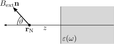
Figure 1: Setup: Neutron in front of an infinite metal or dielectric plate. To lift the degeneracy of the two neutron spin states, an external magnetic field is applied in a direction $\bm{n}(\vartheta)$ which is at an angle $\vartheta$ with respect to the surface normal.

In order to obtain the Casimir–Polder potential of the neutron, we separate the total Hamiltonian into the individual Hamiltonians of the neutron (in the external field $\bm{B}_{\mathrm{ext}}$) and the medium-assisted electromagnetic field on one hand, and the interaction Hamiltonian on the other. We treat the latter as a perturbation. The free field Hamiltonian is given by Buhmann12

$$\hat{H}_{\mathrm{F}}=\int\mathrm{d}^{3}\bm{r}\int_{0}^{\infty}\mathrm{d}\omega\hbar\omega\hat{\bm{f}}^{\dagger}(\bm{r},\omega)\cdot\hat{\bm{f}}(\bm{r},\omega)\,.$$ (1)

Here, $\hat{\bm{f}}^{\dagger}(\bm{r},\omega)$ are bosonic creation operators of effective medium–field excitations. The external (classical) static magnetic field $\bm{B}_{\mathrm{ext}}=B_{\mathrm{ext}}\bm{n}$ splits the energies of the two neutron spin states. Its directional unit vector $\bm{n}$ is at an angle $\vartheta$ with respect to the unit normal of the plate. The resulting Hamiltonian of the neutron in the external magnetic field reads

$$\hat{H}_{\mathrm{N}}=E_{\uparrow}\left|\uparrow\right\rangle\left\langle\uparrow\right|+E_{\downarrow}\left|\downarrow\right\rangle\left\langle\downarrow\right|,$$ (2)

with energies $E_{\uparrow/\downarrow}=\pm(\hbar\gamma_{\mathrm{N}}B_{\mathrm{ext}})/2$. Here, $\gamma_{\mathrm{N}}$ is the gyromagnetic ratio of the neutron, given by $\gamma_{\mathrm{N}}=(g_{\mathrm{N}}e)/(2m_{\mathrm{N}})$ and relates the magnetic dipole moment $\hat{\bm{m}}$ of the neutron to its spin $\hat{\bm{s}}$ via $\hat{\bm{m}}=\gamma_{\mathrm{N}}\hat{\bm{s}}$. $g_{\mathrm{N}}$ is the $g$-factor of the neutron, $m_{\mathrm{N}}$ its mass and $e$ the elementary electric charge. Finally, the interaction Hamiltonian is given by Buhmann12

$$\hat{H}_{\mathrm{int}}=-\hat{\bm{m}}\cdot\hat{\bm{B}}(\bm{r}_{\mathrm{N}})$$ (3)

where $\hat{\bm{B}}$ is the quantised (fluctuating) plate-assisted magnetic field

$$\hat{\bm{B}}(\bm{r})=\sqrt{\frac{\hbar}{\pi\varepsilon_{0}}}\int_{0}^{\infty}\mathrm{d}\omega\,\frac{\omega}{c^{2}}\int\limits\mathrm{d}^{3}\bm{r}^{\prime}\sqrt{\mathrm{Im}\varepsilon(\bm{r^{\prime}},\omega)}\\ \cdot\bm{\nabla}\times\mbox{{{{G}}}}(\bm{r},\bm{r}^{\prime},\omega)\cdot\hat{\bm{f}}(\bm{r}^{\prime},\omega)+\mathrm{h.c.}$$ (4)

Here, $\mbox{{{{G}}}}(\bm{r},\bm{r}^{\prime},\omega)$ is the dyadic Green’s tensor for the classical electromagnetic field that solves the classical boundary problem of the infinite half-space. In other words, the plate represents classical boundary conditions that influence the modes of the quantuised magnetic field $\hat{\bm{B}}$ by means of the classical Green’s tensor $\mbox{{{{G}}}}(\bm{r},\bm{r}^{\prime},\omega)$. The Green’s tensor fulfils the integral relation

$$\frac{\omega^{2}}{c^{2}}\int\mathrm{d}^{3}s\,\operatorname{Im}\,\varepsilon(\bm{s},\omega)\,\mbox{{{{G}}}}(\bm{r},\bm{s},\omega)\!\cdot\!\mbox{{{{G}}}}^{\ast}(\bm{s},\bm{r}^{\prime},\omega)\\ =\operatorname{Im}\,\mbox{{{{G}}}}(\bm{r},\bm{r}^{\prime},\omega)\,.$$ (5)

III Casimir–Polder potential

Starting from an uncoupled state $\left|\{0\}\right\rangle\left|i\right\rangle$, where $\left|\{0\}\right\rangle$ is the vacuum state of the electromagnetic field and $i\in\{\downarrow,\uparrow\}$, we use second-order perturbation theory to find its energy shift

$$U_{i}=\sum_{k=\uparrow,\downarrow}\mathcal{P}\int_{0}^{\infty}\mathrm{d}\omega\dfrac{1}{-\hbar(\omega+\omega_{ki})}\\ \cdot\int\mathrm{d}^{3}\bm{r}\left|\left\langle i\right|\left\langle\{0\}\right|-\hat{\bm{m}}\cdot\hat{\bm{B}}(\bm{r}_{\mathrm{N}})\left|\bm{1}(\bm{r},\omega)\right\rangle\left|k\right\rangle\right|^{2}$$ (6)

where we have defined $\omega_{ik}=(E_{i}-E_{k})/\hbar$. We decompose the potential into $U_{i}=U_{i\downarrow}+U_{i\uparrow}$, where the two terms represent the intermediate state being the spin-down and the spin-up states of the neutron respectively. Using equations (3) and (4) to evaluate the matrix elements of the interaction Hamiltonian, combining the results by means of the integral equation (5) and exploiting Cauchy’s integral formula, one finds

$$U_{\downarrow\downarrow}=U_{\uparrow\uparrow}$$ (7)

$$\hskip 15.93048pt=\dfrac{\mu_{0}}{2}\bm{m}_{\downarrow\downarrow}\cdot\bm{\nabla}\times\mbox{{{{G}}}}^{(1)}(\bm{r}_{\mathrm{N}},\bm{r}_{\mathrm{N}},0)\times\overleftarrow{\bm{\nabla^{\prime}}}\cdot\bm{m}_{\downarrow\downarrow}\,,$$

$$U_{\downarrow\uparrow}=\frac{\mu_{0}}{\pi}\int_{0}^{\infty}\mathrm{d}\xi\dfrac{\omega_{\uparrow\downarrow}}{\xi^{2}+\omega_{\uparrow\downarrow}^{2}}$$ (8)

$$\qquad\times\bm{m}_{\downarrow\uparrow}\cdot\bm{\nabla}\times\mbox{{{{G}}}}^{(1)}(\bm{r}_{\mathrm{N}},\bm{r}_{\mathrm{N}},\omega)\times\overleftarrow{\bm{\nabla^{\prime}}}\cdot\bm{m}_{\uparrow\downarrow}\,,$$

$$U_{\uparrow\downarrow}=-U_{\downarrow\uparrow}$$ (9)

$$\quad+\mu_{0}\bm{m}_{\uparrow\downarrow}\cdot\bm{\nabla}\times\mathrm{Re}\mbox{{{{G}}}}^{(1)}(\bm{r}_{\mathrm{N}},\bm{r}_{\mathrm{N}},\omega_{\uparrow\downarrow})\times\overleftarrow{\bm{\nabla^{\prime}}}\cdot\bm{m}_{\downarrow\uparrow},$$

where the $\bm{m}_{ij}=\left\langle i\right|\hat{\bm{m}}\left|j\right\rangle$ are the magnetic dipole-matrix elements and $\mbox{{{{G}}}}^{(1)}$ is the scattering part of the Green’s tensor. We have used the decomposition $\mbox{{{{G}}}}=\mbox{{{{G}}}}^{(0)}+\mbox{{{{G}}}}^{(1)}$ where the translationally-invariant free-space Green’s tensor $\mbox{{{{G}}}}^{(0)}$ contributes a position-independent energy shift that can be discarded when considering the Casimir–Polder force Buhmann12 . The former can be found by means of rotation operators sakurai and are given by

$$\bm{m}_{\uparrow\uparrow}=-\bm{m}_{\downarrow\downarrow}=\dfrac{\hbar\gamma_{\mathrm{N}}}{2}(\sin\vartheta,0,\cos\vartheta)\,,$$ (10)

$$\bm{m}_{\uparrow\downarrow}=\bm{m}_{\downarrow\uparrow}^{*}=\dfrac{\hbar\gamma_{\mathrm{N}}}{2}(\cos\vartheta,-i,-\sin\vartheta)\,.$$ (11)

In order to calculate the potential further, one has to employ the Green’s tensor corresponding to the setup’s geometry. In the case of the half space, it reads Buhmann12

$$\mbox{{{{G}}}}^{(1)}(\bm{r},\bm{r}^{\prime},\omega)=\dfrac{i}{8\pi^{2}}\\ \cdot\int\dfrac{\mathrm{d}^{2}\bm{k}^{\parallel}}{k^{\perp}}\sum_{\sigma=s,p}r_{\sigma}\bm{e}_{\sigma+}\bm{e}_{\sigma-}e^{i[\bm{k}^{\parallel}\cdot(\bm{r}-\bm{r}^{\prime})+k^{\perp}(z+z^{\prime})]}\,,$$ (12)

where $\bm{k}^{\parallel}$ and $k^{\perp}=\sqrt{(w^{2})/(c^{2})-{\bm{k^{\parallel}}}^{2}}$ are the components of the wave vector $\bm{k}$ which are parallel and perpendicular to the interface. The incident (-) and reflected (+) plane waves as represented by the polarization unit vectors $\bm{e}_{\sigma\pm}$ are polarized parallel ($\sigma=s$) or perpendicular ($\sigma=p$) to the interface and are reflected according to the respective Fresnel reflection coefficients $r_{\sigma}$.

III.1 Perfect conductor

For a perfectly conducting plate with $r_{s}=-r_{p}=-1$, the potential components (7) and (8) simplify to

$$U_{\downarrow\uparrow}=\frac{\hbar^{2}\gamma_{\mathrm{N}}^{2}\mu_{0}}{256\pi^{2}z^{3}}\!\int\limits_{0}^{\infty}\!\frac{\mathrm{d}\xi\,\omega_{\uparrow\downarrow}}{\omega_{\uparrow\downarrow}^{2}+\xi^{2}}[f(\tfrac{\xi z}{c})+\cos 2\vartheta g(\tfrac{\xi z}{c})]e^{-2\xi z/c},$$ (13)

$$U_{\downarrow\downarrow}=\frac{\hbar^{2}\gamma_{\mathrm{N}}^{2}\mu_{0}}{256\pi z^{3}}\left(1+\cos^{2}\vartheta\right)\,.$$ (14)

with $f(x)=5+10x+12x^{2}$ and $g(x)=-1-2x+4x^{2}$. The mixed potential (13) exhibits two different asymptotes in the retarded, $(\omega_{\uparrow\downarrow}z)/c\gg 1$, and the nonretarded regimes, $(\omega_{\uparrow\downarrow}z)/c\ll 1$. They read

$$U^{\mathrm{ret}}_{\downarrow\uparrow}=\dfrac{\hbar^{2}\gamma_{\mathrm{N}}^{2}\mu_{0}c}{32\pi^{2}\omega_{\uparrow\downarrow}z^{4}}\,,$$ (15)

$$U^{\mathrm{nret}}_{\downarrow\uparrow}=\dfrac{\hbar^{2}\gamma_{\mathrm{N}}^{2}\mu_{0}}{512\pi z^{3}}\left(5-\cos 2\vartheta\right)\,.$$ (16)

The potential near a perfect conductor in the nonretarded regime is independent of the magnitude and direction of the external magnetic field and hence also of the neutron spin. It reads

$${\color[rgb]{0,0,0}U_{\mathrm{N}}}=\dfrac{\hbar^{2}\gamma_{\mathrm{N}}^{2}\mu_{0}}{64\pi z^{3}}\equiv\frac{C_{3}^{\text{N}}}{z^{3}}\,.$$ (17)

This result formally agrees with the repulsive potential of a paramagnetic atom in from of a perfectly conducting plate Buhmann12 ,

$$U_{\mathrm{m}}=\frac{\mu_{0}}{48\pi z^{3}}\left\langle\hat{\bm{m}}^{2}\right\rangle,$$ (18)

see also the results of Babiker and Barton for an arbitrary spin particle Babiker72 . For comparison, the potential of an atom $A$ in front of a perfectly conducting plate reads 0022

$$U_{\mathrm{A}}=-\frac{\langle\hat{\bm{d}}^{2}\rangle}{48\pi\varepsilon_{0}z^{3}}\equiv-\frac{C_{3}^{\mathrm{A}}}{z^{3}}\,,$$ (19)

where $C_{3}^{\mathrm{A}}=\langle\hat{\bm{d}}^{2}\rangle/(48\pi\varepsilon_{0})$ is the atomic van der Waals coefficient and $\hat{\bm{d}}$ its electric dipole moment. In an order-of-magnitude estimate, one has $\langle\hat{\bm{d}}^{2}\rangle=e^{2}a_{B}^{2}$ where $a_{B}=(4\pi\varepsilon_{0}\hbar^{2})/(m_{e}e^{2})$ is the Bohr radius and $m_{e}$ is the mass of the electron. Employing $\gamma=(g_{\mathrm{N}}e)/(2m_{\mathrm{N}})$, with $g_{\mathrm{N}}=-3.8$ stocker1994taschenbuch being the $g$-factor of the neutron and $m_{\mathrm{N}}$ being its mass, we find

$$C_{3}^{\mathrm{N}}=\dfrac{3}{16}g_{\mathrm{N}}^{2}\left(\dfrac{m_{e}}{m_{\mathrm{N}}}\right)^{2}\alpha^{2}C_{3}^{\mathrm{A}}\approx 1.7\cdot 10^{-10}C_{3}^{\mathrm{A}}\,,$$ (20)

with $\alpha=e^{2}/(4\pi c\varepsilon_{0}\hbar)\approx 1/137$ being the fine-structure constant. The Casimir–Polder potential of a neutron in front of a perfectly conducting plate is hence ten orders of magnitude smaller than the corresponding potential of a typical atom, which is due to the smallness of the fine structure constant (accounting for roughly four orders) and the small electron-to-neutron mass ratio (accounting for the remaining six orders).

III.2 Metals and dielectrics

To be more realistic, we describe the electric response of the plate by the plasma model, $\varepsilon=1-\omega_{\mathrm{P}}^{2}/\omega^{2}$, the Drude model as given by $\varepsilon=1-\omega_{\mathrm{P}}^{2}/[\omega(\omega+\mathrm{i}\gamma\omega)]$ and a single-resonance Drude–Lorentz model, $\varepsilon=1-\omega_{\mathrm{P}}^{2}/(\omega^{2}-\omega_{\mathrm{T}}^{2})$. Averaging over the direction of the external magnetic field, we find a repulsive ground-state potential for each of these models. As an illustration, we show its constituents and the respective retarded and nonretarded limits for the plasma model in Fig. 2.

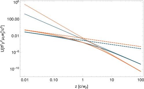
Figure 2: Constituents of the Casimir–Polder potential of a ground-state (spin-down) neutron in front of a surface described by a plasma model with $\omega_{\uparrow\downarrow}=\omega_{P}$: $U_{\downarrow\uparrow}$ (orange) and $U_{\downarrow\downarrow}$ (blue), exact potential (solid), retarded asymptote (dotted) and nonretarded asymptote (dashed).

IV Discussion

In an experiment, applied magnetic fields are typically $B_{\mathrm{ext}}\lesssim 5\mathrm{T}$, such that the critical distance $z_{\mathrm{nret}}=c/\omega_{\uparrow\downarrow}=c/(\gamma_{\mathrm{N}}B_{\mathrm{ext}})\gtrsim 0.32\,\mathrm{m}$ for the nonretarded limit is much larger than typical distances in experiments which vary from $\mathrm{nm}$ to $\mu\mathrm{m}$. We have $z\ll z_{\mathrm{nret}}$, such that we find ourselves in the nonretarded limit. Since each model exhibits its own characteristic frequencies, one can identify different asymptotes for each model where the potential can be described by power laws. The asymptotes together with the corresponding ranges of validity are summarised in Tab. 1. The dispersive parts of these asymptotes with their analogues for magnetic atoms which have previously been reported for metals Henkel05 ; Haakh09 and dielectrics 0831 with two exceptions: our $z\ll z_{\mathrm{critical}}$ asymptote for a Drude metal differs from that given in Refs. Henkel05 ; Haakh09 , because we do not employ a high-frequency cut-off, whereas the $z\gg z_{\mathrm{critical}}$ regime for dielectrics is very specific to neutron interactions and has hence not been considered for atoms.

Model	$\quad U_{\mathrm{N}}(z\ll z_{\mathrm{critical}})$	$\quad U_{\mathrm{N}}(z\gg z_{\mathrm{critical}})$	$z_{\mathrm{critical}}$
I	$\displaystyle\frac{\hbar^{2}\gamma_{\mathrm{N}}^{2}\mu_{0}}{64\pi z^{3}}$		$\displaystyle-$
II	$\displaystyle\frac{\hbar^{2}\gamma_{\mathrm{N}}^{2}\mu_{0}\omega_{p}^{2}}{128\pi c^{2}z}$	$U_{\mathrm{N}}(\mbox{Perf.\ Cond.})$	$\displaystyle\frac{c}{\omega_{\mathrm{P}}}$
III	$\displaystyle-\frac{\hbar^{2}\gamma_{\mathrm{N}}^{2}\mu_{0}\omega_{p}^{2}}{96\pi^{2}c^{2}z}\frac{\gamma_{\mathrm{N}}B_{\mathrm{ext}}}{\gamma}\ln\frac{\gamma_{\mathrm{N}}B_{\mathrm{ext}}}{\gamma}$	$\frac{2}{3}U_{\mathrm{N}}(\mbox{Perf.\ Cond.})$	$\displaystyle\frac{c}{\omega_{\mathrm{P}}}\sqrt{\frac{\gamma}{\gamma_{\mathrm{N}}B_{\mathrm{ext}}}}$
IV	$\displaystyle\frac{\hbar^{2}\gamma_{\mathrm{N}}^{2}\mu_{0}\omega_{\mathrm{P}}^{2}}{192\pi c^{2}}\frac{\omega_{\mathrm{T}}+\omega_{\mathrm{L}}}{\omega_{\mathrm{T}}\omega_{\mathrm{L}}}\dfrac{1}{z}\gamma_{\mathrm{N}}B_{\mathrm{ext}}$	$\displaystyle\frac{\hbar^{2}\gamma_{\mathrm{N}}^{2}\mu_{0}\gamma_{\mathrm{N}}B_{\mathrm{ext}}}{576\pi^{2}cz^{2}}f(\omega_{\mathrm{T}},\omega_{\mathrm{L}})$	$\displaystyle\frac{c}{\omega_{\mathrm{T}}}$

Table 1: Nonretarded ground-state potential $U_{\mathrm{N}}$ for different models (I: Perfect conductor, II: Plasma, III: Drude, IV: Drude–Lorentz) within leading order in the applied magnetic field, valid for $z\ll c/(\gamma_{\mathrm{N}}B_{\mathrm{ext}})$. $\omega_{\mathrm{L}}=\sqrt{\omega_{\mathrm{T}}^{2}+\omega_{\mathrm{P}}^{2}/2}$ and $f(\omega_{\mathrm{L}},\omega_{\mathrm{T}})=(\omega_{\mathrm{L}}^{4}\omega_{\mathrm{T}}^{2}+5\omega_{\mathrm{L}}^{6}-3\omega_{\mathrm{L}}^{2}\omega_{\mathrm{T}}^{4}-\omega_{\mathrm{T}}^{6})/(\omega_{\mathrm{L}}^{4}\omega_{\mathrm{T}}^{2})$.

The asymptotes show that for the perfect conductor and the plasma model, the potential persists even of vanishing external magnetic field. For the two other models instead, the potential vanishes in the limit of vanishing external magnetic field. We note that the different models lead to a variety of asymptotic power laws for the distance dependence. Interestingly, it is seen that the perfect-conductor limit does not commute with the nonretarded limit for the plasma model, in contrast to the case of the Casimir–Polder potential of an electrically polarisable atom 0296 . In addition, there are marked differences between the plasma and Drude models, making this interaction a new and sensitive test case for the Drude–plasma debate in Casimir physics Brevik06 ; Bordag09 . Ultimately, the strong model-dependence of the neutron Casimir–Polder potential stems from its mixed electric–magnetic interaction in a short-distance regime, which is analogous to the case of the anomalous magnetic moment of the electron Bennett13 ; Bennet18 .

Finally, let us discuss whether the potentials predicted for the different models are in principle observable in an experiment. To that end, we compare them with the gravitational potential exerted on the neutron by the same plate and by Earth, respectively, as well as the potential arising from the static electric and magnetic polarisabilities of the neutron. In Fig. 3, the neutron Casimir–Polder potential at accessible distance regimes is shown for the different models alongside the gravitational and static potentials. We see for instance that both the plasma and the Drude model approach the perfect conductor at different critical distances but always are smaller than the latter. The Drude–Lorentz model gives rise to the smallest potential at all distances. The magnitude of the Casimir-Polder potential is highly model-dependent.

Furthermore, while the Casimir–Polder potential is generally weaker than the gravitational potential of Earth except for the perfect-conductor case, it is for all models stronger than the gravitational potential of the plate itself. It should hence be taken into account when performing short-range gravity experiments with neutrons. To estimate the gravitational field of a surface in a typical neutron interferometry experiment Rauch02 , we have for simplicity used a silicon sphere (density $\rho=2.33\,\mathrm{g}/\mathrm{cm}^{3}$) of radius $r=11.3\,\mathrm{mm}$ whose mass is comparable to a plate in a perfect crystal interferometer. For another state-of-the-art neutron setup probing Earth’s gravitation, see e.g. reference Kulin15 .

Static electric and magnetic polarizabilities of the neutron result in the potential 0095

$$U_{\mathrm{static}}=-\frac{3\hbar c(\alpha-\beta)}{8\pi z^{4}},$$ (21)

where $\alpha$ and $\beta$ are the neutron’s static electric and magnetic polarisabilities, respectively ($\alpha=(11.8\pm 1.1)\cdot 10^{-4}\mathrm{fm}^{3}$, $\beta=(3.7\pm 1.2)\cdot 10^{-4}\mathrm{fm}^{3}$ Zyla20 ). The corresponding potential is negative and thus attractive. Its absolute value is shown as a dashed line in Fig. 3. We see that the potential due to static polarisabilities is smaller than the repulsive potential derived in our work, by several orders of magnitude.

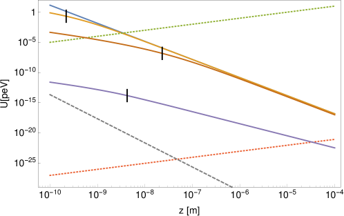
Figure 3: Ground-state Casimir–Polder potential of a neutron in front of a surface with applied field $B_{\mathrm{ext}}=2\,\mathrm{T}$ (solid lines) compared to gravitational potentials (dashed) and the absolute value of the attractive potential due to the neutron’s static electric and magnetic polarisability (dashed): Perfect conductor (blue), plasma model for gold (orange, $\omega_{\mathrm{P}}=1.37\cdot 10^{16}\,\mathrm{rad}/\mathrm{s}$ palik1998handbook ), Drude model for gold (red, $\gamma=4.10\cdot 10^{12}\,\mathrm{rad}/\mathrm{s}$ palik1998handbook ), Drude–Lorentz model for silicon (purple, $\omega_{\mathrm{P}}=2.3\cdot 10^{16}\,\mathrm{rad}/\mathrm{s}$, $\omega_{\mathrm{T}}=7.1\cdot 10^{16}\,\mathrm{rad}/\mathrm{s}$ Pirozenko08 ), gravitational potentials of Earth (green) and of a silicon sphere (red). The black vertical lines represent the critical distances for each model.

By contrast, in gravitational resonance spectroscopy experiments, ultra-cold neutrons form gravitationally bound states above a planar surface which is totally reflecting for neutrons. Currently, transitions between such states can be resolved with $\Delta E\leq 2\cdot 10^{-3}\,$ peV Cronenberg2018 , while near-term experimental setups are expected to achieve $\Delta E\sim 10^{-5}\,$ peV Sedmik2020 . The wave functions of the lowest states probe the space region up to $60\,\mu\mathrm{m}$ above the mirror, with energies in the $\mathrm{peV}$ range, see Appendix A for details. The first-order perturbative energy shift of the gravitational state $\psi_{n}(z)$ due to the Casimir–Polder potential of a mirror described by the plasma model reads

$$\delta E_{\mathrm{CP}}(n) = \int_{z=0}^{\infty}\mathrm{d}z\,|\psi_{n}(z)|^{2}{\color[rgb]{0,0,0}U^{\mathrm{plasma}}_{\mathrm{N}}(z)}.$$ (22)

Note that the integral in equation (22) converges due to the behaviour of the neutron’s wavefunction for small distances. This is not the case when using the perfect conductor model which has to be regularized by including the lattice constant of the half-space medium as a cut-off for small distances, beyond which the continuoum description of the perfect-conductor model breaks down. For currently realized setups Cronenberg2018 ; Cronenberg2015 , the Casimir–Polder interaction predicted by the plasma model would lead to an energy shift of $\Delta E_{\mathrm{CP}}(n,m)=\delta E_{\mathrm{CP}}(n)-\delta E_{\mathrm{CP}}(m)={\color[rgb]{0,0,0}1.7}\cdot 10^{-14}\,\mathrm{peV}$ for the transition $(n,m)=(1,5)$, which is below the detection threshold. This is true even for a planned improved setup involving Ramsey-based gravity resonance spectroscopy Abele2010 with an estimated sensitivity of $\Delta E=5\cdot 10^{-9}\,\mathrm{peV}$ which is statistically limited. The influence of the Casimir–Polder potential can be increased by adding an additional mirror on top, separated from the lower mirror by a distance of a few tens of microns. The two mirrors effectively squeeze the neutron’s wavefunction, leading to an increase of the energy shifts in the transitions by orders of magnitude. For instance, the energy shift of the transition $(1,5)$ is increased by a factor of $200$ (taking a typical mirror spacing of $15\,\mu\mathrm{m}$), see appendix A. While this energy shift still remains under the current detection threshold, future experiments with a sensitivity below the expected energy shift could distinguish between these models. In this case, contributions from the Casimir–Polder potential have to be taken into account. Furthermore, setups whose bound states have a larger neutron density close to the surface would lead to enhanced Casimir–Polder shifts that are cubically enhanced with the inverse distance.

V Conclusions

We have shown that a single neutron under the influence of a constant magnetic field will be subject to a repulsive Casimir–Polder-type dispersion interaction with a metal or dielectric plate. This is a rare example of Casimir repulsion for a magnetisable object interacting with a polarisable one where the repulsion is not dominated by an attractive electric–electric force. We have found that the force is nonretarded for experimentally accessible regimes and that it is very sensitive to the electric response of the surface. It may hence provide a testing ground for the Drude-plasma debate. In addition, while typically smaller than Earth’s gravitational potential by orders of magnitude, it can become comparable to the gravitational interaction of the same surface. Furthermore, we find that while in current neutron experiments, the contribution of Casimir–Polder interactions is not visible, in future high-precision gravitational experiments on short length-scales, a possible influence has to be taken into account.

Appendix A Energy shifts in Gravitational Resonance Spectroscopy experiments

Here we discuss in more detail the influence of the Casimir–Polder potential in Gravitational Resonance Spectroscopy experiments. As discussed above, different gravitational bound states of the neutron experience different energy shifts due to the Casimir–Polder interaction of the neutron with nearby mirrors. For a neutron localised above a totally reflecting mirror, the $n$-th bound state is described by the wavefunction Westphal2007

$$\psi_{n}(z)=c_{A}(n)\operatorname{Ai}(\hat{z}-E(n)),$$ (23)

where $\operatorname{Ai}$ denotes the Airy function of the first kind, $c_{A}(n)$ is a normalization constant, $\hat{z}$ is the rescaled distance to the mirror and $E(n)$ is the rescaled eigenenergy of the bound state. In the case of a double mirror configuration with mirror spacing $l$, the bound wavefunctions are given by Westphal2007

$$\psi_{n}(z)=c_{A}(n,l)\operatorname{Ai}(\hat{z}-E(n,l))+c_{B}(n,l)\operatorname{Bi}(\hat{z}-E(n,l)),$$ (24)

where $\operatorname{Bi}$ is the Airy function of second kind and the rescaled eigenenergies $E(n,l)$ as well as the coefficients $c_{A}(n,l)$ and $c_{B}(n,l)$ now depend on the mirror spacing $l$. A sketch of the wavefunctions for the lowest energy bound states in the double mirror configuration is shown in Fig. 4(a). Note that a penetration of the wavefunctions into the mirror is neglected.

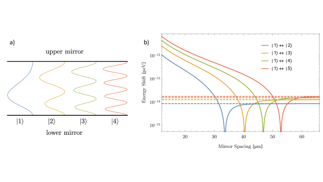
Figure 4: (a) Sketch of the lowest energy bound states of the neutrons in the double mirror configuration. (b) Corrections $|\Delta E_{\mathrm{CP}}(n,m)|$ of the transition energies due to the Casimir–Polder interaction of the neutron in the double mirror configuration as a function of the mirror spacing. Dashed lines indicate the correction of the transition energies for a single-mirror setup. The mirrors are modeled with the plasma model ($\omega_{\mathrm{P}}=1.37\cdot 10^{16}\,\mathrm{rad}/\mathrm{s}$).

Using equation (22), we can now compute first-order energy corrections for transitions between the different bound states. Modeling the reflecting mirrors with the plasma model, we show different transition energies as a function of the mirror spacing $l$ in Fig. 4(b). We see that by varying the mirror spacing, one can manipulate the influence of the Casimir–Polder effect on the different transitions. In particular, for small mirror spacings, the effect is increased by several orders of magnitude with respect to the correction in case of a single-mirror setup (dashed lines).

References

- (1) H. B. G. Casimir, Proc. K. Ned. Akad. Wet. 51, 793 (1948).
- (2) E. M. Lifshitz, Sov. Phys. JETP 2, 73 (1956).
- (3) P. W. Milonni, The Quantum Vacuum (Academic Press, New York, 1994).
- (4) H. B. G. Casimir and D. Polder, Phys. Rev. 73, 360 (1948).
- (5) T. H. Boyer, Phys. Rev. A 9, 2078 (1974).
- (6) V. Hushwater, Am. J. Phys. 65, 381 (1997).
- (7) G. Feinberg and J. Sucher, J. Chem. Phys. 48, 3333 (1968).
- (8) A. Salam, Int. J. Quantum Chem. 78, 437 (2000).
- (9) C. Henkel and K. Joulain, Europhys. Lett. 72, 929 (2005).
- (10) O. Kenneth, I. Klich, A. Mann and M. Revzen, Phys. Rev. Lett. 89, 033001 (2002).
- (11) T. H. Boyer, Phys. Rev. 180, 19 (1969).
- (12) Y. Tikochinsky and L. Spruch, Phys. Rev. A 48, 4236 (1993).
- (13) C. Henkel, B. Power and F. Sols, J. Phys. Conf. Ser. 19, 34 (2005).
- (14) S. Y. Buhmann, D.-G. Welsch and T. Kampf, Phys. Rev. A 72, 032112 (2005).
- (15) H. Safari, D.-G. Welsch, S. Y. Buhmann and S. Scheel, Phys. Rev. A 78, 062901 (2008).
- (16) H. Haakh, F. Intravaia, C. Henkel, S. Spagnolo, R. Passante, B. Power and F. Sols, Phys. Rev. A, 80, 062905 (2009).
- (17) G. Bimonte, G. L. Klimchitskaya and V. M. Mostepanenko Phys. Rev. A 79, 042906 (2009).
- (18) J. E. Lennard-Jones, Trans. Faraday Soc. 28, 333 (1932).
- (19) C. Farina, F. C. Santos and A. C. Tort, J. Phys. A: Math. Gen. 35, 2477 (2002).
- (20) C. Farina, F. C. Santos and A. C. Tort, Am. J. Phys. 70, 421 (2002).
- (21) F. M. Serry, D. Walliser and G. J. Maclay, J. Appl. Phys. 84, 2501 (1998).
- (22) J. N. Munday, F. Capasso and V. A. Parsegian, Nature 457, 170 (2009).
- (23) J. M. Obrecht, R. J. Wild, M. Antezza, L. P. Pitaevskii, S. Stringari and E. A. Cornell, Phys. Rev. Lett. 98, 063201 (2007).
- (24) H. Failache, S. Saltiel, M. Fichet, D. Bloch, M. Ducloy, Phys. Rev. Lett. 83, 5467 (1999).
- (25) F. S. S. Rosa, D. A. R. Dalvit and P. W. Milonni, Phys. Rev. Lett. 100, 183602 (2008).
- (26) F. S. S. Rosa, D. A. R. Dalvit and P. W. Milonni, Phys. Rev. A 78, 032117 (2008).
- (27) S. J. Rahi, M. Kardar and T. Emig, Phys. Rev. Lett. 105, 070404 (2010).
- (28) M. Babiker and G. Barton, Proc. R. Soc. Lond. Ser. A 326, 255 (1972).
- (29) J. F. Babb and M. S. Hussein, EPJ Web of Conferences 113, 08001 (2016).
- (30) J. Baumann, R. Gahler, J. Kalus and W. Mampe, Phys. Rev. D 37, 3107 (1988).
- (31) C. Abel et al, Phys. Rev. Lett. 124, 081803 (2020).
- (32) I. Altarev et al, (2015), J. Appl. Phys. 117, 183903 (2015).
- (33) H. Rauch, H. Lemmel, M. Baron and R. Loidl, Nature 417, 630 (2002).
- (34) S. Y. Buhmann, Dispersion Forces I—Macroscopic Quantum Electrodynamics and Ground-State Casimir, Casimir–Polder and van der Waals Forces (Springer, Heidelberg, 2012).
- (35) J. J. Sakurai, Modern Quantum Mechanics (Addison–Wesley, New York, 1994).
- (36) H. Stöcker, Taschenbuch der Physik, 2nd Ed. (Harri Deutsch, Frankfurt, 1994).
- (37) M. Babiker and G. Barton, J. Phys. A: Math. Gen. 9, 129 (1976).
- (38) I. Brevik, S. A. Ellingsen, K. A. Milton, New J. Phys. 8, 236 (2006).
- (39) M. Bordag, G. L. Klimchitskaya, U. Mohideen, V. M. Mostepanenko, Advances in the Casimir effect (Oxford University Press, Oxford, 2009) and references therein.
- (40) R. Bennett and C. Eberlein, Phys. Rev. A 88, 012107 (2013).
- (41) R. Bennett, S. Y. Buhmann and C. Eberlein, Phys. Rev. A 98, 022515 (2018).
- (42) Palik, E. D. (ed.), Handbook of Optical Constants of Solids III (Academic Press, New York, 1991).
- (43) I. Pirozhenko and A. Lambrecht, Phys. Rev. A 77, 013811 (2008).
- (44) G. V. Kulin, A. I. Frank, S. V. Goryunov, D. V. Kustov, P. Geltenbort, M. Jentschel, A. N. Strepetov and V. A. Bushuev, Nucl. Instrum. Meth. Phys. Res. A 792, 38 (2015).
- (45) P. A. Zyla et al, Prog. Theor. Exp. Phys. 2020, 083C01 (2020).
- (46) G. Cronenberg et al, Nat. Phys. 14 1022 (2018).
- (47) R. Sedmik et al, J. Synch. Investig. 14, 195 (2020).
- (48) G. Cronenberg, H. Filter, M. Thalhammer, T. Jenke, H. Abele and P. Geltenbort, PoS (EPS-HEP2015) 408 (2015).
- (49) H. Abele, T. Jenke, H. Leeb and J. Schmiedmayer, Phys. Rev. D 81, 065019 (2010).
- (50) A. Westphal, H. Abele, S. Baeßler, V. V. Nesvizhevsky, K. V. Protasov and A. Y. Voronin, Eur. Phys. J. C51, 367 (2007).