Where Are Most of the Globular Clusters in Today’s Universe?

Abstract

The total number of globular clusters (GCs) in a galaxy rises continuously with the galaxy luminosity $L$, while the relative number of galaxies decreases with $L$ following the Schechter function. The product of these two very nonlinear functions gives the relative number of GCs contained by all galaxies at a given $L$. It is shown that GCs, in this universal sense, are most commonly found in galaxies within a narrow range around $L_{\star}$. In addition, blue (metal-poor) GCs outnumber the red (metal-richer) ones globally by 4 to 1 when all galaxies are added, pointing to the conclusion that the earliest stages of galaxy formation were especially favorable to forming massive, dense star clusters.

1. Introduction

Galaxies with luminosities higher than $L\sim 10^{7}L_{\odot}$ – in essence, all but the very smallest dwarfs – have measurable numbers of globular clusters (GCs), the massive compact star clusters that were preferentially formed during the earliest stages of star formation during galaxy evolution. The number of GCs present in a given galaxy increases dramatically with host galaxy mass or luminosity, but not in a simple linear way (Harris et al., 2013, hereafter HHA13). At the same time, the relative number of galaxies decreases continuously with $L$ following the empirically based Schechter function (Schechter, 1976).

Combining these two opposing trends leads to a rather simple question: which galaxies contribute the most to the total number of globular clusters in the universe? Dwarf galaxies have very few GCs individually, but there are huge numbers of such galaxies. Contrarily, the biggest GC populations are to be found in central supergiant ellipticals like M87, but these are very rare galaxies. Which ones are the most important when added up over the entire galaxy population?

At the same time, we can address the question of the two classic subpopulations of GCs, the blue (metal-poor) and red (metal-rich) ones that are consistently seen to form a bimodal distribution in GC luminosity versus color (e.g. Brodie & Strader, 2006). Color index increases monotonically with GC metallicity and thus is a useful proxy for [Fe/H], with the dividing line between blue and red near [Fe/H] $\simeq-1$. Whereas the blue GCs are consistently found in all galaxies from dwarfs to giants, the red ones reside preferentially in massive galaxies; quantitative discussions of this trend are given by, e.g., Peng et al. (2006, 2008) and Harris et al. (2015) (hereafter HHH15). Because the metal-poor blue GCs are found in all galaxies, it could therefore be expected that they would outnumber the metal-richer ones in total, but it is not immediately clear by how much.

In this paper, some simple GC demographics are calculated to gain a first answer to these questions. As will be seen below, the discussion draws heavily on recent observational gains that establish the numbers of blue, red, and all GCs within galaxies covering their entire luminosity range (see HHA13, HHA15). In what follows I have adopted a distance scale of $H_{0}=70$ km s^-1 Mpc^-1 wherever necessary.

2. Analysis

In Figure 1, the total number of GCs ($N_{GC}$) is plotted versus host galaxy luminosity ($L$), from data for 418 galaxies of all types as listed in the recent catalog of HHA13. Here, no discrimination is made by galaxy type (spiral, S0, E), but as shown in HHA13 and HHH15, differences by type appear to have only second-order effects. For about half the observed sample (n=216), the original observations are of sufficient photometric precision and depth to resolve the standard bimodal distribution in GC colors and thus to obtain the red and blue fractions as well.

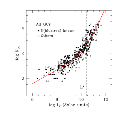
Figure 1.— Total number of globular clusters $N_{GC}$ versus host galaxy luminosity $(L_{V}/L_{\odot})$, with data from the catalog of HHA13. Solid symbols denote galaxies in which the relative numbers of blue (metal-poor) and red (metal-rich) GCs are known, while open symbols denote galaxies in which only the totals have been estimated. The equation for the interpolation curve is given in the text. The vertical dashed line shows $L_{\star}$ from the Schechter function.

For our purposes here, a useful interpolation curve giving the trend of $N_{GC}$ versus $L(gal)$, is

$${\rm log}N_{GC}=\begin{cases}-3.71+0.548x&(x<9.35),\\ -0.30+0.66x-0.1815x^{2}+0.014x^{3}&(x\geq 9.35)\end{cases}$$ (1)

where $x$ = log $(L_{V}/L_{\odot})$. A marked change in the slope of this relation happens near $L\sim 2\times 10^{9}L_{\odot}$; for the dwarfs fainter than that transition we find $N_{GC}\sim L^{0.5}$, while for large galaxies above it we find roughly $N_{GC}\sim L^{1.4}$. The ratio of these two quantities is the classic specific frequency $S_{N}=const(N_{GC}/L_{V})$ (Harris & van den Bergh, 1981), which has a well known characteristic U-shaped dependence on $L$.

In Figure 2, the same relation is shown but now divided into the blue and red subpopulations. The approximate interpolation curves shown in the Figure are, for the blue GCs,

$${\rm log}N_{GC}=\begin{cases}-3.39+0.51x&(x<9.35),\\ 15.418-3.84x+0.25x^{2}&(x\geq 9.35)\end{cases}$$ (2)

and for the red GCs,

$${\rm log}N_{GC}=\begin{cases}-3.75+0.48x&(x<9.35),\\ -13.31+1.50x&(x\geq 9.35)\,.\end{cases}$$ (3)

The Schechter function giving the relative number of galaxies per unit luminosity is

$$\phi(L)dL\,=\,\phi_{o}({L\over L_{\star}})^{\alpha}e^{-(L/L_{\star})}dL\,.$$ (4)

The parameters ($\alpha,L_{\star}$) may empirically depend somewhat on environment, but in this case the goal is simply to track the first-order behavior of GC populations averaged over all environments. The values adopted here are $\alpha=-1.26$ and $L_{\star}=2.77\times 10^{10}L_{\odot}$ from the SDSS DR6 database discussed by Montero-Dorta & Prada (2009); many other versions close to this pair of values can be found in the recent literature, but the precise numbers do not affect the results of the following discussion in any significant way.

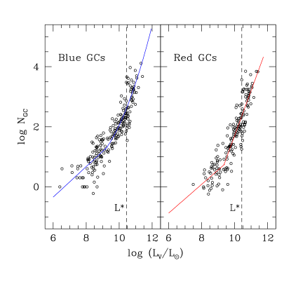
Figure 2.— Left panel: Total number of blue (metal-poor) globular clusters versus host galaxy luminosity; Right panel: total number of red (metal-rich) clusters. The equations for the interpolation curves are given in the text. The vertical dashed lines denote the Schechter-function $L_{\star}$.

Calculating the total number of GCs in all galaxies at a given $L$ is then a matter of multiplying Equation (4) numerically with either (1), (2), or (3) depending on which GC subpopulation we want to track. The results in smoothed histogram form are shown in Figure 3, which gives the total number of GCs in all galaxies within a constant logarithmic bin size $\Delta{\rm log}L=0.01$. In rough terms, this graph gives the relative probability that a globular cluster anywhere in the universe will be sitting in a host galaxy of luminosity (log $L$), or equivalently at a given absolute magnitude.

The shapes of all three curves in Fig. 3 peak strongly at intermediate luminosities very near $L_{\star}$, with a long gradual ramp down towards the dwarf galaxies at lower $L$. Dwarf galaxies are very common but they do not have enough GCs per galaxy to dominate the totals; and contrarily, the highest$-L$ supergiant ellipticals have tens of thousands of GCs each but they are too rare to dominate. What is perhaps surprising is the height and relative sharpness of the population peak. Specifically, we find the following features:

• For all GCs combined, the peak is at log $(L/L_{\odot})\simeq 10.53$ and 50% of the population lies in the range log $(L/L_{\odot})=9.86-10.95$ (a factor of 12 in $L$).

• For the blue GCs, the peak is at log $(L/L_{\odot})\simeq 10.5$ and 50% of the population lies between log $(L/L_{\odot})=9.78-10.93$ (a factor of 14).

• For the red GCs, the peak is at log $(L/L_{\odot})\simeq 10.6$ and 50% of them lie between log $(L/L_{\odot})=10.03-10.99$ (a factor of 9).

The reason why these peaks are rather high and narrow can be seen from Figs. 1 and 2. $N_{GC}$ begins rising steeply near log $(L/L_{\odot})\sim 9.5$, which is still a decade below $L_{\star}$. Thus the Schechter function is still on the flat part of its curve ($L<L_{\star}$) and the number of galaxies at a given $L$ is declining only slowly. Once $L$ passes $L_{\star}$, however, the number of host galaxies declines so steeply that it forces all the curves in Fig. 3 rapidly downward. In short, the galaxies near $L_{\star}$ provide the “best compromise” situation for GC populations in a universal sense: they have typically several hundred GCs per galaxy, and are still numerous enough cosmologically to dominate the GC totals.

The general appearance of Fig. 3 to some extent resembles the Li & White (2009) model calculation of the total amount of stellar mass contributed by galaxies of a given luminosity or baryonic mass (see their Fig. 5). In both cases the distribution is sharply peaked near $\L_{\star}$. However, the long tail towards low $L$ for the GC numbers is noticeably more prominent than for all stellar mass, reflecting the empirical fact that dwarf galaxies have higher average specific frequencies than $L_{\star}$-type ones.

For comparison, Figure 4 presents the cumulative distribution. Half the population of blue GCs resides in galaxies with $L<1.3\times 10^{10}L_{\odot}$, whereas half the red GC population falls within galaxies with $L<2.8\times 10^{10}L_{\odot}$, a crossing point more than twice as high.

It is also noteworthy from Fig. 4 that the blue, metal-poor GCs make up almost 80% of all globular clusters in the universe. A major reason for this predominance is that in the dwarf-galaxy regime (log $(L/L_{\odot}\lesssim 9.5$) there are almost no metal-rich GCs present, and it is only in the very luminous (and rare) supergiants that they make up comparable numbers to the metal-poor ones (see, e.g., Peng et al., 2006; Harris, 2009; Harris et al., 2014, for recent examples).

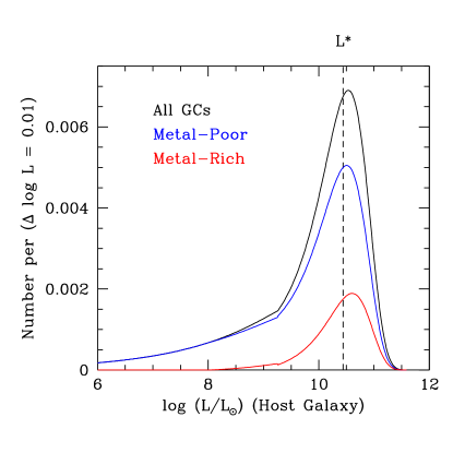
Figure 3.— Relative number of globular clusters in all galaxies at a given luminosity (log $L$). The numbers are for a constant bin size $\Delta{\rm log}L=0.01$ ($\Delta M_{V}=0.025$ magnitude). The values are normalized so that the total integrated over all $L$ equals 1. Black curve: the distribution for all GCs combined, regardless of metallicity; Blue curve: the distribution for only the metal-poor (blue) GCs; and Red curve: the distribution for only the metal-rich (red) GCs. The sum of the blue and red curves by definition equals the upper curve. The vertical dashed line denotes the Schechter-function $L_{\star}$.

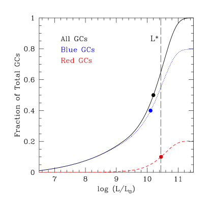
Figure 4.— The fraction of all globular clusters within galaxies with luminosities $\leq L$. The large solid dots indicate the halfway points along each curve; i.e. half the clusters are found in galaxies with $L\leq L_{\bullet}$ in each case. The vertical dashed line denotes the Schechter-function $L_{\star}$.

In Figure 5, another version of the probability distribution is shown, but now plotted versus galaxy halo mass $M_{h}$ rather than luminosity; $M_{h}$ is dominated by dark matter. The Figure shows the total mass in GCs within all galaxies at a given $M_{h}$ rather than the total number, but these are nearly equivalent given the very shallow increase of mean GC mass with galaxy mass (HHA13). This graph was generated through the combination of (a) a double-Schechter-function form of the number of galaxies per unit stellar mass $M_{\star}$, from (Kelvin et al., 2014), (b) conversion of $M_{\star}$ to $M_{h}$ via the stellar-to-halo mass ratio SHMR with the convenient parametrization of Guo et al. (2010), and finally (c) the total mass in GCs within a galaxy of a given $M_{h}$, which has a simple linear form (HHH15).

The graph indicates that GCs are most likely to be found within galaxy halos near $\sim 10^{13}M_{\odot}$, but the peak is much broader than in Fig. 3, a result of the very nonlinear conversion of $M_{\star}$ (baryonic mass) to $M_{h}$. The slight upturn of the curve for $\lesssim 10^{11}M_{\odot}$ is quite uncertain (see HHH15 for a discussion of the data), but is partly determined by the steeper slope of the double Schechter function for the smallest dwarfs (Kelvin et al., 2014). However, this calculation is more or less arbitrarily cut off below $M_{h}=10^{10}M_{\odot}$, since dwarfs below this limit have $<1$ GC each according to the empirical evidence (see HHH15).

Figure 5.— Total mass in all GCs within galaxies at a given halo mass $M_{h}$. The numbers are for a constant bin size $\Delta{\rm log}M_{h}=0.01$. The values are normalized so that the total integrated over all $L$ equals 1. Black curve: the distribution for all GCs combined, regardless of metallicity; Blue curve: the distribution for only the metal-poor (blue) GCs; and Red curve: the distribution for only the metal-rich (red) GCs. The sum of the blue and red curves by definition equals the upper curve. The vertical dashed line denotes the Schechter-function $L_{\star}$.

3. Summary and Discussion

In this paper some broad-brush demographics of globular cluster populations are discussed; for the first time, it is possible to estimate quantitatively (though admittedly only to first order) which galaxies are responsible for contributing most of the GCs in the present-day universe. The combination of the nonlinear shapes of both the $N_{GC}$ versus $L$ function, and the Schechter function for galaxy numbers, demonstrates that galaxies in a narrow range around the Schechter $L_{\star}$ contribute the most.

Expressed in terms of galaxy halo mass (i.e. total mass) rather than luminosity, GCs are predominantly found within halos in the broad range $\sim 10^{12-14}M_{\odot}$, with the peak near $10^{13}M_{\odot}$.

The primary result of this discussion is shown in Fig. 3. It should be seen essentially as a snapshot in time, valid only for the present day: as the universe evolves and the continual process of galaxy merging continues, the biggest galaxies grow by absorbing their small neighbors. Thus over time, the peak in Fig. 3 will shift to higher $L$ and the tail at lower $L$ will shrink. In the past at much higher redshift, the galaxy population was much more dominated by dwarfs and the GC population peak was correspondingly at lower $L$.

The result that the metal-poor GCs outnumber the metal-richer ones by a global ratio of roughly 4 to 1 is striking. The implication for galaxy evolution is that the very earliest stages of hierarchical merging, when baryonic matter was predominantly in quite low-metallicity gas, was exceptionally favorable for the formation of dense massive star clusters (see also Kruijssen, 2015). The bulk of low-metallicity GC formation appears to have happened near $z\sim 5$ (e.g. VandenBerg et al., 2013; Forbes et al., 2015, and references cited there), while the metal-richer “red” population predominated later near $z\sim 2-3$, much nearer the peak of the cosmic star formation rate (e.g. Madau & Dickinson, 2014). At that later time, the remaining gas was much more enriched, but it was not as successful at producing the extremely dense $\sim 10^{5}-10^{7}M_{\odot}$ protocluster clouds within which GCs could form (Harris & Pudritz, 1994; Kravtsov & Gnedin, 2005; Elmegreen et al., 2012; Li & Gnedin, 2014; Kruijssen, 2015).

In the discussion above, the term “globular cluster” is taken implicitly to mean classically old, massive star clusters. If we broaden that definition to include massive star clusters formed at any time, then it would be appropriate to include YMCs (young massive star clusters, also sometimes referred to as super star clusters in the literature) formed in low-redshift mergers between galaxies, as is seen in nearby active merger remnants (e.g. Trancho et al., 2014, 2007; Whitmore et al., 2014; Goudfrooij, 2012; Zepf et al., 1999; Carlson et al., 1998, among others). These young GCs will add to the metal-rich GC population and to some extent increase their fraction of the universal population. However, even in the most prominent mergers (see the citations above for examples) only some dozens of clusters are added that are $\gtrsim 10^{5}M_{\odot}$ and thus likely to survive for many Gyr. These will not add significantly to the old clusters already present when added up over all galaxies. In essence, the GC production in any merger old or young will depend critically on the amount of cold gas available, so most GC formation happened in the early universe (see Li & Gnedin, 2014, for discussion).

Lastly, the present discussion does not account for GCs either in the Intergalactic Medium (IGM) or Intracluster Medium (ICM), i.e. ones not definitely associated with any individual galaxy. True IGM clusters far from any galaxy are extremely hard to find and their numbers are generally presumed to be be very small, lacking any evidence to the contrary. ICM populations of GCs are also not well studied as yet, but are known to exist in a few rich clusters of galaxies such as Virgo or Coma (Peng et al., 2011; Durrell et al., 2014; West et al., 2011; Alamo-Martínez et al., 2013). The cases studied so far indicate that these ICM GCs add up to roughly the same numbers as are associated with the central Brightest Cluster Galaxy in their local environment, and would therefore not change the totals estimated here significantly.

References

- Alamo-Martínez et al. (2013) Alamo-Martínez, K. A., Blakeslee, J. P., Jee, M. J., Côté, P., Ferrarese, L., González-Lópezlira, R. A., Jordán, A., Meurer, G. R., Peng, E. W., & West, M. J. 2013, ApJ, 775, 20
- Brodie & Strader (2006) Brodie, J. P. & Strader, J. 2006, ARA&A, 44, 193
- Carlson et al. (1998) Carlson, M. N., Holtzman, J. A., Watson, A. M., Grillmair, C. J., Mould, J. R., Ballester, G. E., Burrows, C. J., Clarke, J. T., Crisp, D., Evans, R. W., Gallagher, III, J. S., Griffiths, R. E., Hester, J. J., Hoessel, J. G., Scowen, P. A., Stapelfeldt, K. R., Trauger, J. T., & Westphal, J. A. 1998, AJ, 115, 1778
- Durrell et al. (2014) Durrell, P. R., Côté, P., Peng, E. W., Blakeslee, J. P., Ferrarese, L., Mihos, J. C., Puzia, T. H., Lançon, A., Liu, C., Zhang, H., Cuillandre, J.-C., McConnachie, A., Jordán, A., Accetta, K., Boissier, S., Boselli, A., Courteau, S., Duc, P.-A., Emsellem, E., Gwyn, S., Mei, S., & Taylor, J. E. 2014, ApJ, 794, 103
- Elmegreen et al. (2012) Elmegreen, B. G., Malhotra, S., & Rhoads, J. 2012, ApJ, 757, 9
- Forbes et al. (2015) Forbes, D. A., Pastorello, N., Romanowsky, A. J., Usher, C., Brodie, J. P., & Strader, J. 2015, MNRAS, 452, 1045
- Goudfrooij (2012) Goudfrooij, P. 2012, ApJ, 750, 140
- Guo et al. (2010) Guo, Q., White, S., Li, C., & Boylan-Kolchin, M. 2010, MNRAS, 404, 1111
- Harris (2009) Harris, W. E. 2009, ApJ, 699, 254
- Harris et al. (2015) Harris, W. E., Harris, G. L., & Hudson, M. J. 2015, ApJ, 806, 36
- Harris et al. (2013) Harris, W. E., Harris, G. L. H., & Alessi, M. 2013, ApJ, 772, 82
- Harris et al. (2014) Harris, W. E., Morningstar, W., Gnedin, O. Y., O’Halloran, H., Blakeslee, J. P., Whitmore, B. C., Côté, P., Geisler, D., Peng, E. W., Bailin, J., Rothberg, B., Cockcroft, R., & Barber DeGraaff, R. 2014, ApJ, 797, 128
- Harris & Pudritz (1994) Harris, W. E. & Pudritz, R. E. 1994, ApJ, 429, 177
- Harris & van den Bergh (1981) Harris, W. E. & van den Bergh, S. 1981, AJ, 86, 1627
- Kelvin et al. (2014) Kelvin, L. S., Driver, S. P., Robotham, A. S. G., Taylor, E. N., Graham, A. W., Alpaslan, M., Baldry, I., Bamford, S. P., Bauer, A. E., Bland-Hawthorn, J., Brown, M. J. I., Colless, M., Conselice, C. J., Holwerda, B. W., Hopkins, A. M., Lara-López, M. A., Liske, J., López-Sánchez, Á. R., Loveday, J., Norberg, P., Phillipps, S., Popescu, C. C., Prescott, M., Sansom, A. E., & Tuffs, R. J. 2014, MNRAS, 444, 1647
- Kravtsov & Gnedin (2005) Kravtsov, A. V. & Gnedin, O. Y. 2005, ApJ, 623, 650
- Kruijssen (2015) Kruijssen, J. M. D. 2015, MNRAS, 454, 1658
- Li & White (2009) Li, C. & White, S. D. M. 2009, MNRAS, 398, 2177
- Li & Gnedin (2014) Li, H. & Gnedin, O. Y. 2014, ApJ, 796, 10
- Madau & Dickinson (2014) Madau, P. & Dickinson, M. 2014, ARA&A, 52, 415
- Montero-Dorta & Prada (2009) Montero-Dorta, A. D. & Prada, F. 2009, MNRAS, 399, 1106
- Peng et al. (2011) Peng, E. W., Ferguson, H. C., Goudfrooij, P., Hammer, D., Lucey, J. R., Marzke, R. O., Puzia, T. H., Carter, D., Balcells, M., Bridges, T., Chiboucas, K., del Burgo, C., Graham, A. W., Guzmán, R., Hudson, M. J., Matković, A., Merritt, D., Miller, B. W., Mouhcine, M., Phillipps, S., Sharples, R., Smith, R. J., Tully, B., & Verdoes Kleijn, G. 2011, ApJ, 730, 23
- Peng et al. (2006) Peng, E. W., Jordán, A., Côté, P., Blakeslee, J. P., Ferrarese, L., Mei, S., West, M. J., Merritt, D., Milosavljević, M., & Tonry, J. L. 2006, ApJ, 639, 95
- Peng et al. (2008) Peng, E. W., Jordán, A., Côté, P., Takamiya, M., West, M. J., Blakeslee, J. P., Chen, C.-W., Ferrarese, L., Mei, S., Tonry, J. L., & West, A. A. 2008, ApJ, 681, 197
- Schechter (1976) Schechter, P. 1976, ApJ, 203, 297
- Trancho et al. (2007) Trancho, G., Bastian, N., Miller, B. W., & Schweizer, F. 2007, ApJ, 664, 284
- Trancho et al. (2014) Trancho, G., Miller, B. W., Schweizer, F., Burdett, D. P., & Palamara, D. 2014, ApJ, 790, 122
- VandenBerg et al. (2013) VandenBerg, D. A., Brogaard, K., Leaman, R., & Casagrande, L. 2013, ApJ, 775, 134
- West et al. (2011) West, M. J., Jordán, A., Blakeslee, J. P., Côté, P., Gregg, M. D., Takamiya, M., & Marzke, R. O. 2011, A&A, 528, A115
- Whitmore et al. (2014) Whitmore, B. C., Chandar, R., Bowers, A. S., Larsen, S., Lindsay, K., Ansari, A., & Evans, J. 2014, AJ, 147, 78
- Zepf et al. (1999) Zepf, S. E., Ashman, K. M., English, J., Freeman, K. C., & Sharples, R. M. 1999, AJ, 118, 752