Melting of a nonequilibrium vortex crystal in a fluid film with polymers: elastic versus fluid turbulence

Abstract

We perform a direct numerical simulation (DNS) of the forced, incompressible two-dimensional Navier-Stokes equation coupled with the FENE-P equations for the polymer-conformation tensor. The forcing is such that, without polymers and at low Reynolds numbers Re, the film attains a steady state that is a square lattice of vortices and anti-vortices. We find that, as we increase the Weissenberg number Wi, a sequence of nonequilibrium phase transitions transforms this lattice, first to spatially distorted, but temporally steady, crystals and then to a sequence of crystals that oscillate in time, periodically, at low Wi, and quasiperiodically, for slightly larger Wi. Finally, the system becomes disordered and displays spatiotemporal chaos and elastic turbulence. We then obtain the nonequilibrium phase diagram for this system, in the ${\mbox{Wi}}-\Omega$ plane, where $\Omega\propto\mbox{Re}$, and show that (a) the boundary between the crystalline and turbulent phases has a complicated, fractal-type character and (b) the Okubo-Weiss parameter $\Lambda$ provides us with a natural measure for characterizing the phases and transitions in this diagram.

I Introduction

The equilibrium melting transition, from a spatially periodic crystal to a homogeneous liquid, has been studied extensively Ramakrishnan and Yussouff (1979); Haymet (1987); Chaikin and Lubensky (2000); Oxtoby (1991); Singh (1991); Perlekar and Pandit (2010). Nonequilibrium analogs of this transition have been explored in, e.g., the melting of colloidal crystals by shear Das et al. (2002) and the turbulence-induced melting of a periodic array of vortices and anti-vortices in a forced, two-dimensional (2D), fluid film Perlekar and Pandit (2010). We elucidate, via extensive direct numerical simulations (DNSs), the nonequilibrium melting of a periodic array of vortices and anti-vortices in a forced, 2D, fluid film with polymer additives; we refer to this periodic array as a nonequilibrium, 2D crystal; this is also called a cellular flow Gotoh and Yamada (1984, 1987) in some studies.

We show that such a crystal can be melted either (a) by increasing the Reynolds numbers Re or (b) by increasing the Weissenberg number Wi. Case (a) can be thought of as a nonequilibrium melting transition, which is driven by fluid turbulence Perlekar and Pandit (2010); Ouellette and Gollub (2007, 2008) and in which the disordered phase is a turbulent fluid that shows dissipation reduction, because of the polymer additives Perlekar et al. (2010, 2006); Gupta et al. (2015). Case (b) is also a nonequilibrium melting transition; in this case the vortex crystal melts into a disordered state, which is a polymeric fluid that shows elastic turbulence Groisman and Steinberg (2000, 2001) or rheochaos Ganapathy and Sood (2006); Majumdar and Sood (2011). We show that this system of driven vortices and anti-vortices provides an excellent laboratory for studying the crossover from the dissipation-reduction to the elastic-turbulence regimes in a fluid film.

Case (a), namely, turbulence-induced melting, has been explored in experiments Ouellette and Gollub (2007, 2008), which use a spatially periodic force to impose a nonequilibrium vortex crystal on a fluid film at low Re; this crystal melts, at high Re, into a disordered, nonequilibrium, liquid-type phase. This melting problem has been studied by using linear-stability analysis Gotoh and Yamada (1984, 1987), for the first instability of the vortex crystal, and direct numerical simulations (DNS) Perlekar and Pandit (2010); Braun et al. (1997); Molenaar et al. (2007). These DNSs have explored the nonequilibrium phase diagram of this driven, dissipative system by using techniques from nonlinear dynamics Perlekar and Pandit (2010); Braun et al. (1997); Molenaar et al. (2007) and generalizations of order parameters that are used to characterize equilibrium crystals Ramakrishnan and Yussouff (1979); Haymet (1987); Chaikin and Lubensky (2000); Perlekar and Pandit (2010).

To the best of our knowledge, case (b), namely, elastic-turbulence-induced melting of a vortex crystal, has not been explored in experiments, even though there have been several experimental studies of elastic turbulence Groisman and Steinberg (2000, 2001) and the related phenomenon of rheochaos Ganapathy and Sood (2006); Majumdar and Sood (2011). Direct numerical simulations of 2D fluid films with polymer additives have begun to explore the Berti et al. (2008); Berti and Boffetta (2010) elastic-turbulence-induced melting of spatially periodic flows; the Kolmogorov-flow pattern investigated in Ref. Berti et al. (2008); Berti and Boffetta (2010) is a one-dimensional crystal.

The nonequilibrium vortex crystal, whose melting we study, is a 2D crystal. To describe the ordering in this crystal and its subsequent melting, either by elastic or fluid turbulence, we follow the treatment of Ref. Perlekar and Pandit (2010), which has investigated this problem in the absence of polymers. In particular, we solve the incompressible, 2D, Navier-Stokes (NS) equation, for the fluid film, coupled to the FENE-P equation, for the polymer-conformation tensor $\mathcal{C}$; this provides a good description of our system if we can neglect the film thickness and the Marangoni effect, and if the Mach number is low Perlekar and Pandit (2010); Chomaz and Cathalau (1990); Chomaz (2001); Perlekar and Pandit (2009). The force we use yields, at low Re, a spatially periodic array of vortices and antivortices that is stationary in time; we call this a vortex crystal.

As we increase either (a) the forcing amplitude and, thereby Re or (b) the polymer-relaxation time $\tau_{P}$ and, hence, Wi, this crystal loses stability and gives way to a variety of nonequilibrium states. We show that time series of the energy of the fluid, their power spectra, and Poincaré maps help us to understand the spatiotemporal evolution of this system and its sequence of nonequilibrium transitions (cf., Refs. Perlekar and Pandit (2010); Braun et al. (1997); Molenaar et al. (2007) for turbulence-induced melting in a fluid film without polymers).

Our exploration of these transitions, which is inspired by the density-functional theory of the crystallization of a liquid Ramakrishnan and Yussouff (1979); Chaikin and Lubensky (2000); Oxtoby (1991); Singh (1991); Perlekar and Pandit (2010), is based on order parameters for our vortex crystal. The crystal density is periodic in space; the density-functional theory uses its Fourier coefficients as order parameters.

We follow Ref. Perlekar and Pandit (2010) and use the Okubo-Weiss field $\Lambda\equiv\det(A)$ in the vortex-crystal instead of the crystal density $\rho({\bf r})$, in the density-functional theory mentioned above; $A$ has elements $A_{ij}\equiv\partial_{i}u_{j}$, with $u_{j}$ the $j^{th}$ component of the velocity. The Okubo-Weiss criterion Okubo (1970); Weiss (1991), first developed to characterize the local topology of inviscid, incompressible, 2D, fluid flow, is also useful if viscosity and air-drag-induced friction are present Perlekar and Pandit (2009); Rivera et al. (2001); Elhmaïdi et al. (1993); this criterion states that $\Lambda>0$, where the flow is vortical, and $\Lambda<0$, where it is extensional or strain-dominated Okubo (1970); Weiss (1991). In a nonequilibrium vortex crystal, $\Lambda({\bf r})$ has the Fourier expansion

$$\Lambda({\bf r})=\sum_{\bf k}{\hat{\Lambda}}_{\bf k}\exp(\imath{\bf k}\cdot{\bf r}),$$ (1)

where ${\bf k}$ are the reciprocal-lattice vectors and the ${\hat{\Lambda}}_{\bf k}$ are the natural order parameters for the vortex crystal. In our 2D vortex crystal, the counterpart of the structure factor $S({\bf k})$, for a crystal Ramakrishnan and Yussouff (1979); Chaikin and Lubensky (2000); Oxtoby (1991); Singh (1991); Perlekar and Pandit (2010), is the 2D spectrum

$$E_{\Lambda}({\bf k})\equiv\langle{\hat{\Lambda}}_{\bf k}{\hat{\Lambda}}_{\bf-k}\rangle,$$ (2)

where the angular brackets denote the average over the nonequilibrium state of our system (and not a Gibbsian thermal average); this state can (a) be independent of time, (b) exhibit periodic or quasiperiodic oscillations, or (c) be spatiotemporally chaotic and turbulent, but statistically steady. We define

$$G({\bf r})=\langle\overline{\Lambda({\bf x+r})\Lambda({\bf x})}\rangle,$$ (3)

an autocorrelation function whose spatial Fourier transform is related to $E_{\Lambda}({\bf k})$. This characterizes the spatial correlations in our system (the overbar in Eq. 3 indicates the average over the origin ${\bf x}$). As we show below, the near isotropy of the turbulent phase implies that, to a very good approximation, $G$ depends only on $r\equiv\mid{\bf r}\mid$ here; and it characterizes the short-range vortical order in our 2D fluid film, exactly as the density correlation function $g(r)$ does in an isotropic liquid at equilibrium Ramakrishnan and Yussouff (1979); Chaikin and Lubensky (2000); Oxtoby (1991); Singh (1991); Perlekar and Pandit (2010). We also follow the spatiotemporal evolution of the polymer-conformation tensor ${\cal C}$ and relate it to the spatiotemporal evolution of $\Lambda$.

We use the order parameters, defined above, to obtain many interesting results for the elastic-turbulence-induced melting of such a 2D vortex crystal in a fluid film with polymer additives. We first describe our principal results qualitatively. We show that, as Re or Wi increase, the steady, ordered, vortex crystal proceeds to the disordered, turbulent state via a sequence of nonequilibrium transitions between different nonequilibrium phases, which we list in Table 1 (column four): SX is the original, temporally steady, crystal, with a square unit cell that is imposed by the force; this is followed by phases of type SXA, which are temporally steady crystals that are distorted relative to SX; we then find distorted crystals that displays periodic (OPXA) or quasiperiodic (OQPXA) oscillations in time; finally, the system exhibits spatiotemporal chaos and turbulence (SCT). We conjecture that OPXA and OQPXA are actually several (perhaps an infinity) different nonequilibrium spatiotemporal crystals, which are periodic in space and time; given the spatial and temporal resolutions of our calculation, we can identify only some of these. In addition to the order parameters and correlation functions mentioned above, we also examine the spatiotemporal evolution of the polymer-conformation tensor $\mathcal{C}$ in these phases. Our work leads to a rich, nonequilibrium phase diagram for our system. This has not been studied hitherto.

The remainder of this paper comprises the following Sections. Section 2, which is devoted to the equations that we use to model 2D fluid films with polymer additives and the numerical methods we employ. Section 3 contains our results. Section 4 is devoted to a discussion of our results and to conclusions.

II Model and Numerical Methods

To study a 2D fluid film with polymer additives, we write the 2D, incompressible, NS and FENE-P equations in terms of the streamfunction $\psi$ and the vorticity $\omega=\nabla\times\bf u(\bf x,t)$, where ${\bf u}\equiv(-\partial_{y}\psi,\partial_{x}\psi)$ is the fluid velocity at the point $\bf x$ and time $t$, as follows (we use the nondimensional form suggested in Ref. Platt et al. (1991) for 2D fluid films without polymer additives):

$$D_{t}{\bf\omega} = \nabla^{2}{\bf\omega}/{\Omega}+\frac{\beta}{\Omega\mbox{Wi}}\nabla\times\nabla.[f(r_{P}){\cal C}]-\alpha\omega+F_{\omega};$$ (4)

$$\nabla^{2}{\bf\psi} = {\bf\omega};$$ (5)

$$D_{t}{\cal C} = {\cal C}.(\nabla{\bf u})+{(\nabla{\bf u})^{T}}.{\cal C}-\frac{{f(r_{P}){\cal C}}-{\cal I}}{\mbox{Wi}};$$ (6)

here, $D_{t}\equiv\partial_{t}+{\bf u}\cdot\nabla$, the uniform solvent density $\rho=1$, $\alpha$ is the non-dimensionalized, air-drag-induced friction coefficient, $\beta=\mu/\nu$, the Weissenberg number ${\mbox{Wi}}=\tau_{P}(F_{amp}/(nk\nu))$, $\nu$ is the kinematic viscosity, $\mu$ the zero-shear viscosity parameter for the solute (FENE-P), $\tau_{P}$ the polymer relaxation time, and $F_{\omega}\equiv-n^{3}[\cos(nx)+\cos(ny)]/\Omega$ is the non-dimensionalized, spatially periodic force, whose injection wave vector is related to $n$, $\alpha=n\nu\alpha^{\prime}k/F_{amp}$, and $\Omega=nF_{amp}/(\nu^{2}k^{3})=n{\mbox{Re}}$, where $F_{amp}$ is the forcing amplitude, and $\alpha^{\prime}$ is the coefficient of friction, Re is the Reynolds number. We non-dimensionalize lengths by a factor $k/n$, with $k$ a wave number or inverse length Platt et al. (1991). The $x$ and $y$ components of the velocity are $u_{1}\equiv u$ and $u_{2}\equiv v$, respectively. The superscript $T$ denotes a transpose, ${\cal C}_{\alpha\beta}\equiv{\langle{R_{\alpha}}{R_{\beta}}\rangle}$ are the elements of the polymer-conformation tensor (angular brackets indicate the average over polymer configurations), the identity tensor ${\cal I}$ has the elements $\delta_{\alpha\beta}$, $f(r_{P})\equiv{(L^{2}-2)/(L^{2}-r_{P}^{2})}$ is the FENE-P potential that ensures finite extensibility, and $r_{P}\equiv\sqrt{{\rm Tr}(\cal C)}$ and $L$ are, respectively, the length and the maximal possible extension of the polymers.

Our direct numerical simulation (DNS) of Eqs. (4)-(6) uses the MPI code that we have developed to study fluid turbulence with polymer additives in fluid films Gupta et al. (2015). We use periodic boundary conditions, a square simulation domain of side ${\mathbb{L}}=2\pi$, and $N^{2}$ collocation points; these boundary conditions are well suited for studying vortex crystals with square unit cells. We use a fourth-order, Runge-Kutta scheme, with time step $\delta t$, for time marching and an explicit, fourth-order, central-finite-difference scheme in space and the Kurganov-Tadmor (KT) shock-capturing scheme Kurganov and Tadmor (2000) for the advection term in Eq. (6), because this scheme (see Eq. (7) of Ref. Perlekar et al. (2010)) successfully resolves steep gradients in ${\cal C}_{\alpha\beta}$ and, thereby, minimizes dispersion errors. We solve the Poisson equation (5) in Fourier space by using a pseudospectral method and the FFTW library Frigo and Johnson (1999). We choose $\delta t$ to be small enough to prevent $r_{P}$ from becoming larger than $L$ (if $r_{P}>L$, there is a numerical instability). To preserve the symmetric-positive-definite (SPD) nature of $\cal C$ at all times we adapt to 2D the Cholesky-decomposition scheme of Refs. Perlekar et al. (2010, 2006); Gupta et al. (2015); Vaithianathan and Collins (2003). In particular, we define ${\cal J}\equiv f(r_{P}){\cal C}$, so Eq. (6) becomes

$$D_{t}{\cal J}={\cal J}.(\nabla{\bf u})+({\nabla\bf u})^{T}.{\cal J}-s({\cal J}-{\cal I})+q{\cal J},$$ (7)

where $s=(L^{2}-2+j^{2})/(\tau_{P}L^{2})$, $q=[d/(L^{2}-2)-(L^{2}-2+j^{2})(j^{2}-2)/(\tau_{P}L^{2}(L^{2}-2))]$, $j^{2}\equiv Tr({\cal J})$, and $d=Tr[{\cal J}.(\nabla{\bf u})+(\nabla{\bf u})^{T}.{\cal J}].$ Note that ${\cal C}$, and hence ${\cal J}$, are SPD matrices, so ${\cal J}={\cal LL}^{T}$, where ${\cal L}$ is a lower-triangular matrix with elements $\ell_{ij}$, such that $\ell_{ij}=0$ for $j>i$. We can now use Eq.(7) to obtain, for $1\leq i\leq 2$ and $\Gamma_{ij}=\partial_{i}u_{j},$

$${D_{t}\ell_{11}} = \Gamma_{11}\ell_{11}+\Gamma_{21}\ell_{21}+\frac{1}{2}\Big{[}(q-s)\ell_{11}+\frac{s}{\ell_{11}}\Big{]},$$

$${D_{t}\ell_{21}} = \Gamma_{12}\ell_{11}+\Gamma_{21}\frac{\ell_{22}^{2}}{\ell_{11}}+\Gamma_{22}\ell_{21}$$

$${}+\frac{1}{2}\Big{[}(q-s)\ell_{21}-s\frac{\ell_{21}}{\ell^{2}_{11}}\Big{]},$$

$${D_{t}\ell_{22}} = -\Gamma_{21}\frac{\ell_{21}\ell_{22}}{\ell_{11}}+\Gamma_{22}\ell_{22}$$ (8)

$${}+\frac{1}{2}\Big{[}(q-s)\ell_{22}-\frac{s}{\ell_{22}}\left(1+\frac{\ell^{2}_{21}}{\ell^{2}_{11}}\right)\Big{]}.$$

Equation(8) preserves the SPD property of $\cal C$ if $\ell_{ii}>0$; we enforce this, as in Refs. Perlekar et al. (2010, 2006); Gupta et al. (2015), by considering the evolution of $\ln(\ell_{ii})$ instead of $\ell_{ii}$.

In most of our studies, we use a time step $\delta t=10^{-3}$ to $10^{-4}$ for $N=128$; its precise value depends on the value of the polymer-relaxation time $\tau_{P}$; for $\tau_{P}\simeq 1$, $\delta t=10^{-3}$ and $\delta t=10^{-4}$ otherwise ($\tau_{P}>1$). Our results do not change significantly if we use $N=256$ or $N=1024$ (we have checked this in representative cases). We obtain long time series for several variables (see below) to make sure that the temporal evolution of our system is captured accurately; most of our runs are at least as long as $5\times 10^{6}\delta t$. We monitor the time-evolution of the total kinetic energy $E(t)\equiv\overline{{\bf u}^{2}}$ and calculate the stream function $\psi$, vorticity $\omega$, polymer-conformation tensor $\mathcal{C}$, the Okubo-Weiss parameter $\Lambda$, and the kinetic energy spectrum $E(k)\equiv\sum_{k-1/2<k^{\prime}\leq k+1/2}k^{\prime 2}\langle|\hat{\bf\psi}({\bf k^{\prime}},t)|^{2}\rangle_{t}$, where $\langle\rangle_{t}$ indicates the time average over the statistically steady state. From these we obtain $E_{\Lambda}({\bf k})$ and $G({\bf r})$, by averaging over $40$ configurations of $\Lambda({\bf r})$, which are separated from each other by $10^{5}\delta t$; to eliminate the effects of initial transients, we remove data from the first $10^{6}$ time steps before we collect data for these averages. From $\psi$ we obtain the velocity and thence the ${\bf k}=(1,0)$ component of the Fourier transform $\hat{v}$ of the $y$ component $v$ of ${\bf u}$. We use the time series of $E(t)$ to obtain its temporal Fourier transform $E(f)$ and from that the power spectrum $\mid E(f)\mid$, which we use to differentiate between periodic, quasiperiodic, and chaotic temporal evolutions. We also use Poincaré-type sections, namely, plots of $\Im\hat{v}_{(1,0)}$ versus $\Re\hat{v}_{(1,0)}$ at successive times (for the Kolmogorov flow see Ref. Platt et al. (1991)).

The equation of motion for a small, rigid particle (henceforth, an inertial particle) in an incompressible flow Maxey and Riley (1983); Gatignol (1983) assumes the following simple form Bec et al. (2006); Boffetta et al. (2004), if the particle is much heavier than the advecting fluid:

$$\frac{d{\bm{x}}}{dt}={\bm{v}}(t);\frac{d{\bm{v}}}{dt}=-\frac{{\bm{v}}(t)-{\bf u}[{\bm{x}}(t),t]}{\tau_{\rm s}};$$ (9)

here, ${\bm{v}}$ and ${\bm{x}}$ are, respectively, the velocity and position of an inertial particle, $\tau_{\rm s}=(2a^{2})/(9\nu\rho_{\rm f})$ is the Stokes or response time of the particle, whose ratio with the Kolmogorov dissipation time $T_{\eta}$ is the Stokes number ${\rm St}=\tau_{\rm s}/T_{\eta}$. We assume that the radius of a particle $a\ll\eta$, where $\eta$ is the dissipation scale of the carrier fluid, and that the particle density is so low that we can neglect interactions between particles. We also assume, as in Ref. De Lillo et al. (2012), that the polymer additives affect the inertial-particle velocity ${\bm{v}}(t)$ only by virtue of their effect on the Eulerian velocity ${\bf u}[{\bm{x}}(t),t]$ of the fluid at the position of the inertial particle. We show below that the spatial distribution of such inertial particles in the flow can also be used to distinguish the nonequilibrium crystalline and turbulent states in our system.

III Results

We now present the results of our DNS. We begin with an overview, in the first subsection. In the next subsection, we present the nonequilibrium phase diagram that we obtain from our calculations. We then present the results of our numerical simulations for $n=4$ and the ranges of parameters given in Table 1. In the third and fourth subsections, respectively, we present our results for $\Omega=1$ and $\Omega=22$. In the fifth subsection, we report our results for the order parameters, spatial correlation functions, and kinetic-energy spectra that we have defined above; and the last subsection contains our results for the spatial patterns of polymers and inertial particles.

III.1 Overview

We demonstrate below how our crystal of vortices melts, as we increase Wi for a fixed, low value of $\Omega$, through a sequence of transitions. At somewhat higher values of $\Omega$, at which the vortex crystal has already reached a melted state because of fluid turbulence, we find that this turbulent state moves first to a frozen state, as we increase Wi; this frozen state melts again as Wi increases some more. The air-drag-induced friction delays these transitions; we have checked this in some representative cases. However, to make contact with earlier studies of turbulence-induced melting of a vortex crystal Perlekar and Pandit (2010); Braun et al. (1997); Molenaar et al. (2007) without polymers, we do not include air-drag-induced friction here; our conclusions are not altered qualitatively by this.

The steady-state solution Platt et al. (1991); Perlekar and Pandit (2010), of Eq. (4) is $\omega_{s,n}=-n[\cos(nx)+\cos(ny)]$, if $\mbox{Wi}=0$ and $\Omega<\Omega_{s,n}$; here the subscript $s$ stands for steady state. We examine the destabilization of this solution, by increasing Wi, while we hold $\Omega$ fixed, for one representative value of $n$, namely, $n=4$ for which $\Omega_{s,4}\simeq 5.657$ (see Ref. Perlekar and Pandit (2010)). The initial vorticity is taken to be $\omega=\omega_{s,n}+10^{-4}\sum_{m_{1}=0,m_{2}=0}^{2,2}[\sin(m_{1}x+m_{2}y)+\cos(m_{1}x+m_{2}y)]m_{2}^{2}/\sqrt{(m_{1}^{2}+m_{2}^{2})}$; and the system then evolves under the force $F_{\omega}$. For a fixed value of $\Omega$, we increase Wi in steps of $0.1$; and we carry out simulations for $\Omega=1,2$, and from then to $\Omega=26$ in steps of $2$. To track the nonequilibrium transitions in our system, say from SXA to SCT, we have also carried out runs in which we increase Wi in steps of $\simeq 0.01$. We have validated our numerical scheme by comparing our results with those of Refs. Platt et al. (1991); Perlekar and Pandit (2010). Reference  Platt et al. (1991) studies a Kolmogorov flow $F_{\omega}=n\cos(ny)$; and Ref. Perlekar and Pandit (2010) uses an external force of the form $F_{\omega}\equiv-n^{3}[\cos(nx)+\cos(ny)]/\Omega$, which is exactly the same as the one we employ.

$Run$	$\Omega$	Wi	$\rm{Order}$
${\tt R1-1}$	$1$	$\mbox{Wi}\leq 1.9$	$\rm{SX}$
${\tt R1-2}$	$1$	$2\leq\mbox{Wi}\leq 9$	$\rm{OPXA}$
${\tt R1-3}$	$1$	$\mbox{Wi}\geq 10$	$\rm{SCT}$
${\tt R22-1}$	$22$	$\mbox{Wi}=0$	$\rm{SCT}$
${\tt R22-2}$	$22$	$0<\mbox{Wi}<0.45$	$\rm{OPXA}$
${\tt R22-3}$	$22$	$\mbox{Wi}=0.5$	$\rm{SXA}$
${\tt R22-4}$	$22$	$0.55<\mbox{Wi}<0.8$	$\rm{OPXA}$
${\tt R22-5}$	$22$	$\mbox{Wi}\geq 1$	$\rm{SCT}$

Table 1: Table indicating the number of the Run (e.g., R1-1), the value of $\Omega$, and the type of order. SX : original, steady square crystal (the pattern depends on $n$); SXA : temporally steady crystals slightly distorted compared to SX; OPXA : crystal that is distorted slightly relative to SX and with temporal oscillations; OQPXA : OPXA but with quasiperiodic temporal oscillations; SCT : disordered phase with spatiotemporal chaos and turbulence. We have carried out $\simeq 400$ such Runs.

For $\mbox{Wi}=0$ and $\Omega<\Omega_{s,n}$, the $\Lambda$ field shows alternating vortical and extensional regions, which are also referred to as centers and saddles; these are arranged in a two-dimensional square lattice, which we illustrate via pseudocolor plots of $\Lambda$, for $n=4$, in Fig. 1 (a). For $\Omega=20$, which is well beyond $\Omega_{s,4}\simeq 5.657$, the fluid becomes turbulent; but, on the addition of polymers, Wi increases, and the fluid again forms a 2D vortex lattice, which we illustrate via pseudocolor plots of $\Lambda$, for $n=4$, in Fig. 1 (b). In Figs. 2 (a) and (b) we show the corresponding pseudocolor plots of the streamfunction $\psi$.

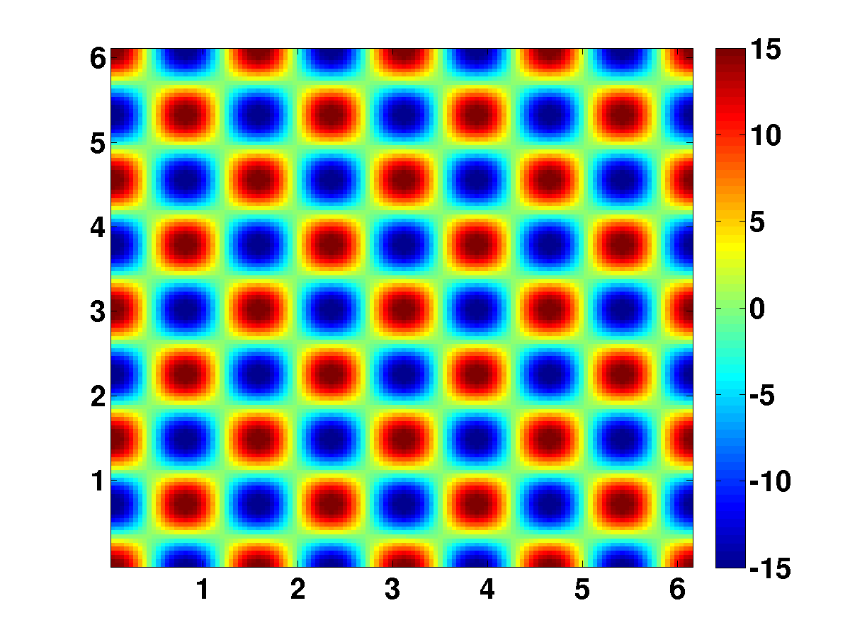
Figure 1: (Color online) Pseudocolor plots of the Okubo-Weiss parameter $\Lambda$ for (a) $\Omega=1$ and $\mbox{Wi}=0$ and (b) $\Omega=20$ and $\mbox{Wi}=1$; these show vortex-crystal states. Given our color bar in (a), vortical regions are red and strain-dominated regions are dark blue.

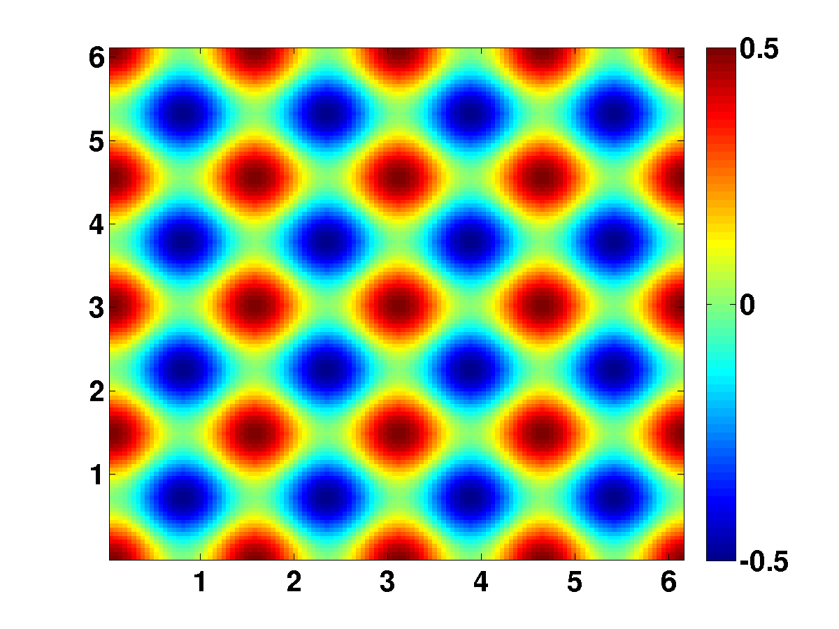
Figure 2: (Color online) Pseudocolor plots of the stream function $\psi$, illustrating vortex-crystal states, for (a) $\Omega=1$ and $\mbox{Wi}=0$ and (b) $\Omega=20$ and $\mbox{Wi}=1$.

III.2 Nonequilibrium Phase Diagram

We have carried out a very large number ($\simeq 400$) of DNS studies of our system for a wide range of parameter values in the $(\mbox{Wi}$-$\Omega)$ plane; only a very small fraction of these parameter values are listed in Table 1. For each one of these parameter sets we calculate the quantities, such as $E(t)$, which we have defined above; and from these calculations we obtain the rich, nonequilibrium phase diagram of Fig. 3 (a), in which blue circles represent the steady crystal SXA, green circles represent either temporally periodic (OPXA) or quasiperiodic (OQPXA) states, and the red circles represent the state SCT that displays spatiotemporal chaos and turbulence. The most striking feature of this nonequilibrium phase diagram is that the boundaries between the different states are very complicated, with a fractal-type interleaving of the states SXA, OPXA/OQPXA, and SCT; this is especially clear in Fig. 3(b), which shows a detailed view of the phase diagram in the vicinity of the these boundaries. Earlier studies of elastic turbulence seem to have missed the complicated nature of these boundaries because they have not been able to examine these transition in as much detail as we have done.

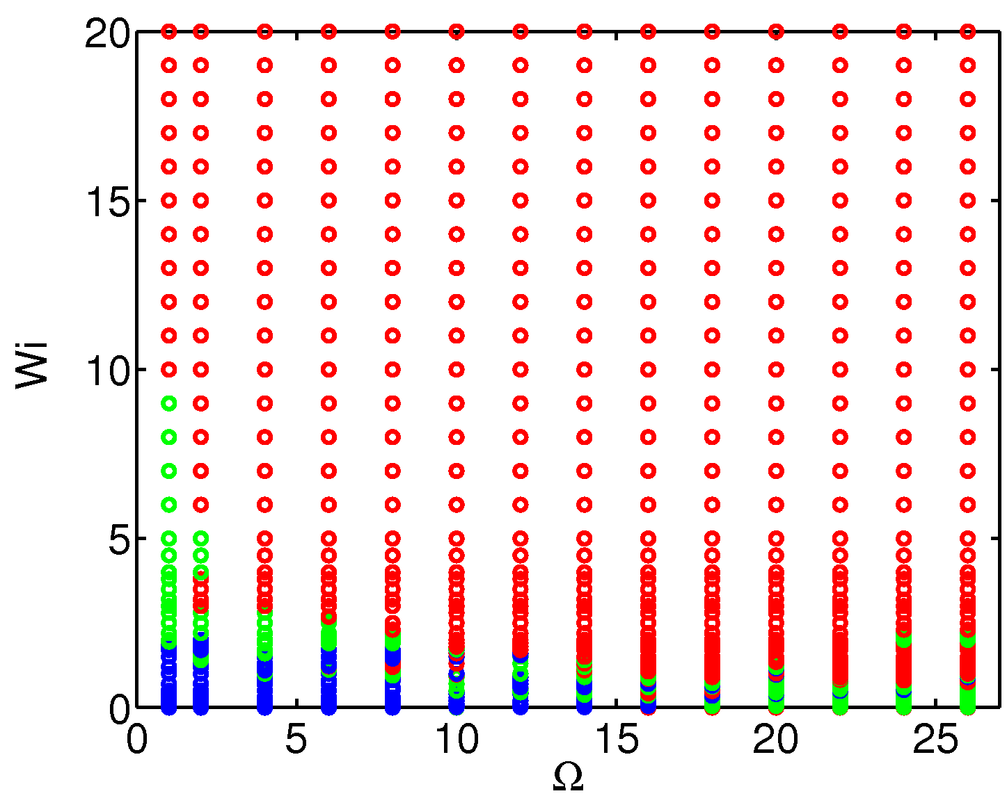
Figure 3: (Color online) (a) Phase diagram of our 2D system with polymer additives in the Wi-$\Omega$ plane, where blue circles represent the regions SX and SXA, green circles represent the regions OPXA and OQPXA, and the red circles represents the region SCT; (b) an enlarged version of a region of the phase diagram in (a).

Fractal-type boundaries between different nonequilibrium states have been obtained in nonequilibrium phase diagrams for some other extended dynamical systems. Examples of such boundaries can be found in the transition to turbulence in pipe flow Schneider et al. (2007), the transitions between different spiral-wave patterns in mathematical models for cardiac tissue Shajahan et al. (2007, 2009), and the transition from no-dynamo to dynamo regimes in a shell model for magnetohydrodynamic (MHD) turbulence Sahoo et al. (2010). In many dynamical systems, a fractal basin boundary can separate the basin of attraction of a fixed point or a limit cycle from the domain of attraction of a strange attractor; thus, a small change in the initial condition can lead either to the simple dynamical evolutions, associated with fixed points or limit cycles, or to chaos, because of a strange attractor. The 2D Navier-Stokes (NS) and FENE-P equations that we study here comprise a $4N^{2}$-dimensional dynamical systems, where $N^{2}$ is the number of grid points; the factor of $4$ appears here because we have the 2D vorticity and the three independent components of the $\cal L$ matrix at each grid point. It is not feasible to find the complete basin boundaries for such a high-dimensional dynamical system (we use $N\sim 10^{2}$ so $4N^{2}\sim 4\times 10^{4}$); however, we can reasonably assume that complicated, fractal-type boundaries separate the basins of attraction of the SXA, OPXA/OQPXA, and SCT states. Note that we do not change the initial condition; instead, we change our dynamical system by changing the parameters $F_{amp}$ and $\tau_{P}$ and, hence, ${\Omega}$ and Wi. This change affects the long-time evolution of our 2D NS and FENE-P system as sensitively as does a change in the initial conditions because the fractal basin boundary itself changes with these parameters. Reference Schneider et al. (2007) has found such a sensitive dependence on model parameters in the transition to turbulence and the edge of chaos in pipe flow (see their Fig. 3, which shows that the border, in parameter space, between the laminar and turbulent regions is very complicated, in much the same way as the phase boundary is in our study). In Refs. Shajahan et al. (2007, 2009), it has been shown that the spatiotemporal evolution of spiral waves of electrical activation depends sensitively on inhomogeneities in partial-differential-equation models for ventricular tissue; changes in the positions of these inhomogeneities in models for cardiac tissue correspond in our system to changes in parameters such as $\Omega$ and Wi. A shell-model study of the dynamo transition in MHD has also found such a fractal-type boundary, separating dynamo and no-dynamo regimes, in the plane of the magnetic Reynolds number and the magnetic Prandtl number Sahoo et al. (2010).

In the next two subsections we describe in detail the results of our calculations for two representative values of $\Omega$, namely, $1$ and $22$, and a range of values of Wi (Table 1). We have carried out many such calculations ($\simeq 400$) to obtain the phase diagram of Fig. 3.

III.3 The case $\Omega=1$

If $\Omega=1$, which lies in region $\Omega<\Omega_{s,n=4}$, the steady-state solution is $\omega_{s,n=4}$, in the absence of polymers. When we add FENE-P polymers to the 2D Navier-Stokes fluid and increase the Weissenberg number Wi, the steady-state solution $\omega_{s,n=4}$ becomes unstable. For the range of values of Wi in our runs ${\tt R1-1}$ (Table 1), we obtain a steady vortex crystal, which is shown by the pseudocolor plots of $\psi$ and $\Lambda$ in Figs. 4(a) and (b), respectively, for the illustrative value $\mbox{Wi}=1$; for this set of parameters, Fig. 4(c) shows the reciprocal-space spectrum $E_{\Lambda}$, which has clear, dominant peaks at the forcing wave vectors.

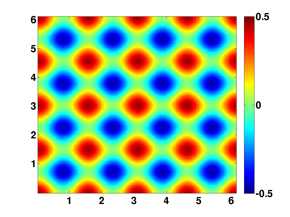
Figure 4: (Color online) Pseudocolor plots for $\Omega=1$ and $\mbox{Wi}=1$ : (a) the streamfunction $\psi$ and (b) the Okubo-Weiss parameter $\Lambda$; (c) a filled contour plot of the $E_{\Lambda}$, reciprocal-space spectrum; this shows peaks at the forcing wave vectors.

As we increase Wi beyond $1.9$, new dynamical regimes appear in the range of values for our runs $\tt R1-2$. In particular, we observe, for $\Omega=1$ and $\mbox{Wi}=3$, that the time series of $E(t)$ is periodic (Fig. 5 (a)) and its power spectrum $|E(f)|$ (Fig. 5(b)) shows one dominant peak, with hardly any sign of higher harmonics. Thus, the Poincaré-type map in the $(\Re[\hat{v}(1,0)],\Im[\hat{v}(1,0)])$ plane (Fig. 5(c)) displays a simple attractor. In Figs. 5(d) and (e), we show, for these parameter values, pseudocolor plots of $\psi$ and $\Lambda$, respectively; there is spatial undulation in the former and the latter is deformed relative to SX (Fig. 1(a)). In the reciprocal-space spectrum $E_{\Lambda}$ (Figure 5(f)), we do not see any major peaks, other than the ones at the forcing wave vectors, because the deformation of the original crystal is weak; the amplitudes of these dominants peaks are smaller than those of their counterparts, at the forcing wave vectors, in Fig.4(c).

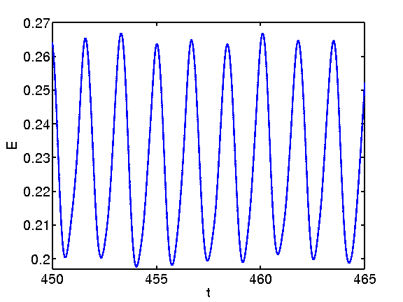
Figure 5: (Color online) Plots, for $\Omega=1$ and $\mbox{Wi}=3$ : (a) the time evolution of the energy $E(t)$, (b) its power spectrum $|E(f)|$ versus the frequency $f$, and (c) the Poincaré-type section in the plane $(\Re[\hat{v}(1,0)],\Im[\hat{v}(1,0)])$. Pseudocolor plots of (d) the streamfunction $\psi$, (e) the Okubo-Weiss parameter $\Lambda$, and (f) a filled contour plot of the reciprocal-space spectrum $E_{\Lambda}$; the amplitudes of the principal peaks in (f) are lower than the amplitudes of their counterparts, at the forcing wave vectors, in Fig. 4(c).

An additional increase of Wi (runs ${\tt R1-3}$ with $\mbox{Wi}>10$) leads to chaotic temporal evolution and a disordered set of vortices and antivortices in space. Thus, we have states with spatiotemporal chaos and turbulence; for our nonequilibrium system, turbulent states with spatiotemporal chaos are the analogs of the disordered liquid state, which appears on the melting of an equilibrium crystal Ramakrishnan and Yussouff (1979); Haymet (1987); Chaikin and Lubensky (2000); Oxtoby (1991); Singh (1991); Perlekar and Pandit (2010). We illustrate a state with spatiotemporal chaos for $\Omega=1$ and $\mbox{Wi}=20$ by the plots in Fig. 6. In particular, Fig. 6(a) shows the chaotic energy time series $E(t)$, whose power spectrum $|E(f)|$ (Fig 6(b)) shows a broad background, which indicates temporal chaos. The scattered points in the Poincaré-type section in the $(\Re[\hat{v}(1,0)],\Im[\hat{v}(1,0)])$ plane confirm the presence of chaos. The disorder of this state is shown in the pseudocolor plots of $\psi$ and $\Lambda$ in Figs. 9(d) and (e), respectively; and the associated reciprocal-space spectrum $E_{\Lambda}({\bf k})$ (Fig. 9(f)) shows many new Fourier modes in addition to the residual peaks at the forcing wave vectors.

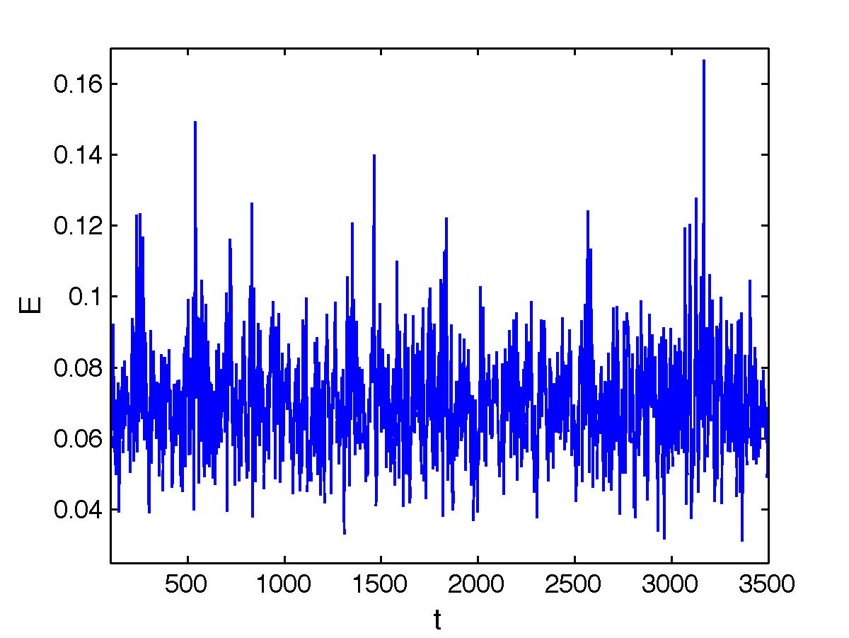
Figure 6: (Color online) Plots for $\Omega=1$ and $\mbox{Wi}=20$ : (a) the time evolution of the energy $E(t)$, (b) its power spectrum $|E(f)|$ versus the frequency $f$, and (c) the Poincaré-type section in the plane $(\Re[\hat{v}(1,0)],\Im[\hat{v}(1,0)])$. Pseudocolor plots of (d) the streamfunction $\psi$ and (e) the Okubo-Weiss parameter $\Lambda$; and (f) a filled contour plot of the reciprocal-space spectrum $E_{\Lambda}$, which shows that various Fourier modes are present in addition to those at the forcing wave vectors.

Thus, we see that the onset of elastic turbulence can lead to vortex-crystal melting, through a very rich sequence of transitions, even when $\Omega$ is itself too small to melt this nonequilibrium crystal. The spatial autocorrelation function $G({\bf r})$ and the evolution of the order parameters $\langle{\hat{\Lambda}_{\bf k}}\rangle$ with Wi are given in the fifth subsection.

III.4 The case $\Omega=22$

If we do not have any polymers and if $\Omega=22$, which is greater than $\Omega_{s,n=4}$, the steady-state solution $\omega_{s,n=4}$ is unstable, and the temporal evolution of our system is chaotic as we can see from the time series of the energy in Fig. 7(a). Its power spectrum $|E(f)|$, which is plotted in Fig. 7(b), has several peaks in a broad background, and the Poincaré-type section in the $(\Re[\hat{v}(1,0)],\Im[\hat{v}(1,0)])$ (Fig. 7 (c)) displays points that cover a two-dimensional area. The disordered spatial structure of this state, shown by the pseudocolor plots of $\psi$ and $\Lambda$ in Figs. 7 (d) and (e), respectively, indicates that this state is spatiotemporally chaotic and turbulent. Figure 7 (f) shows the reciprocal-space energy spectrum $E_{\Lambda}$, which exhibits a large number of Fourier modes in addition to the ones at the forcing wave vectors.

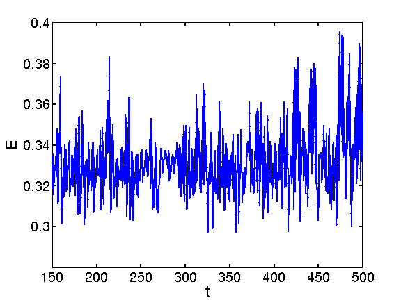
Figure 7: (Color online) Plots for $\Omega=22$ and $\mbox{Wi}=0$ : (a) the time evolution of the energy $E(t)$, (b) its power spectrum $|E(f)|$ versus the frequency $f$, and (c) the Poincaré-type section in the plane $(\Re[\hat{v}(1,0)],\Im[\hat{v}(1,0)])$. Pseudocolor plots of (d) the streamfunction $\psi$ and (e) the Okubo-Weiss parameter $\Lambda$; and (f) a filled contour plot of the reciprocal-space spectrum $E_{\Lambda}$, which shows a large number of Fourier modes in addition to the ones at the forcing wave vectors.

When we add polymers to our 2D Navier-Stokes system at $\Omega=22$, these polymers lead first to a reappearance of states that are periodic in time; this occurs, e.g., for the range of Wi covered in runs $\tt R22-2$. For $\mbox{Wi}=0.3$, Fig. 8(a) shows that time series of the energy is periodic in time and its power spectrum $|E(f)|$ (Fig. 8(b)) has a fundamental peak at $f_{0}=2.5\times 10^{-3}$ and harmonics at $f_{1}=2f_{0}$, $f_{2}=3f_{0}$, $f_{4}=4f_{0}$, and $f_{5}=5f_{0}$. The Poincaré-type section in the $(\Re[\hat{v}(1,0)],\Im[\hat{v}(1,0)])$ plane in Fig. 8 (c) exhibits a simple attractor, which is consistent with the periodic behaviors that emerge from Figs. 8(a) and (b). The spatial organization of this state, shown by pseudocolor plots of $\psi$ and $\Lambda$ in Figs. 8 (d) and (e), respectively, is disordered, although some vestiges of the unit cells of the original crystal are visible in the pseudocolor plot of $\Lambda$; and Fig. 8 (f) shows the reciprocal-space spectrum $E_{\Lambda}$.

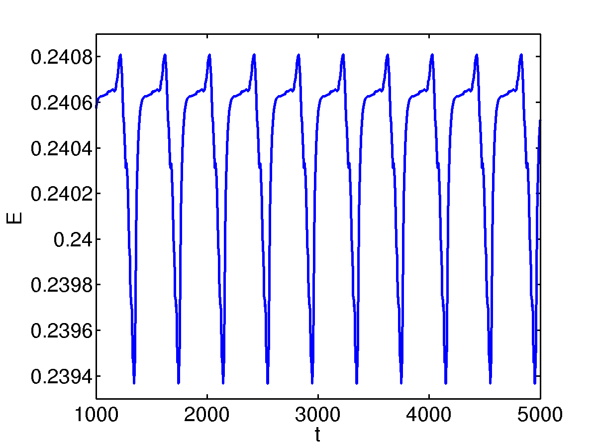
Figure 8: (Color online) Plots for $\Omega=22$ and $\mbox{Wi}=0.3$ : (a) the time evolution of the energy $E(t)$, (b) the power spectrum $|E(f)|$ versus the frequency $f$, and (c) the Poincaré-type section in the plane $(\Re[\hat{v}(1,0)],\Im[\hat{v}(1,0)])$. Pseudocolor plots of (d) the streamfunction $\psi$ and (e) the Okubo-Weiss parameter $\Lambda$; (f) a filled contour plot of the reciprocal-space spectrum $E_{\Lambda}$.

If we increase the Weissenberg number to $\mbox{Wi}=0.5$ in run $\tt R22-3$, we obtain a new steady state that is a vortex crystal; however, it is not exactly the same as the original vortex crystal as can be seen clearly by comparing the pseudocolor plots of $\Lambda$ in Figs. 1(a) and  9(b). This difference is even more striking if we compare the pseudocolor plots of $\psi$ shown in Figs. 9(a) and 2(a). Not surprisingly, then, the reciprocal-space energy spectrum $E_{\Lambda}$ shows new peaks in addition to the ones at the forcing wave vectors, which now appear with a reduced amplitude.

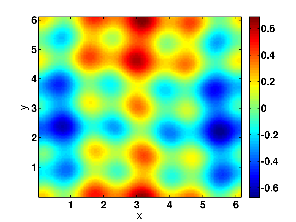
Figure 9: (Color online) Pseudocolor plot for $\Omega=22$ and $\mbox{Wi}=0.5$ : (a) the streamfunction $\psi$ and (b) the Okubo-Weiss parameter $\Lambda$; and (c) a filled contour plot of the reciprocal-space spectrum $E_{\Lambda}$, which shows peaks at the forcing wave vectors, but with amplitudes that are lower than for their counterparts in Fig.4(c).

If we increase Wi some more (runs $\tt R22-4$ with $0.55\leq\mbox{Wi}\leq 0.8$), we obtain a spatiotemporal crystal, i.e., one that is spatially periodic and which also oscillates in time Perlekar and Pandit (2010). For instance, if $\mbox{Wi}=0.7$, the time series of the energy is periodic in time, as shown in Fig. 10(a); and Fig. 10(b) shows that its power spectrum $|E(f)|$ has only one dominant peak, which is a clear indication that the temporal evolution is periodic. Figure 10(c) shows the Poincaré-type section in the $(\Re[\hat{v}(1,0)],\Im[\hat{v}(1,0)])$ plane, which displays that the projection of the attractor on this plane is a closed loop. Figures 10(d) and (e) show pseudocolor plots of $\psi$ and $\Lambda$, respectively; and the associated reciprocal-space spectrum $E_{\Lambda}$ (Fig. 10(f)) shows dominant peaks principally at the forcing wave vectors.

Figure 10: (Color online) Plots for $\Omega=22$ and $\mbox{Wi}=0.7$ : (a) the time evolution of the energy $E(t)$, (b) the power spectrum $|E(f)|$ versus the frequency $f$, and (c) the Poincaré-type section in the plane $(\Re[\hat{v}(1,0)],\Im[\hat{v}(1,0)])$. Pseudocolor plots of (d) the streamfunction $\psi$ and (e) the Okubo-Weiss parameter $\Lambda$; and (f) a filled contour plot of the reciprocal-space spectrum $E_{\Lambda}$.

We now increase Wi again (run $\tt R22-5$); the temporal evolution of the system becomes chaotic and the spatial organization of the vortex crystal is distorted. Thus, we finally enter a state with spatiotemporal chaos and turbulence (SCT); this is our analog of the disordered, liquid state, which appears on the melting of an equilibrium crystal Ramakrishnan and Yussouff (1979); Chaikin and Lubensky (2000); Oxtoby (1991); Singh (1991). However, some vestiges of the incipient crystalline ordering can still be found in reciprocal-space spectra, as we illustrate for $\mbox{Wi}=20$ in Fig. 11. From the time series $E(t)$ of the energy (Fig. 11(a)), it is clear that system is chaotic; this is confirmed by the power spectrum $|E(f)|$ (Fig. 11(b)), which displays several peaks, and the Poincaré-type section in the $(\Re[\hat{v}(1,0)],\Im[\hat{v}(1,0)])$ plane (Fig. 11(c)), in which the points fill a two-dimensional area. The disordered spatial organization of vortical structures is shown in Figs. 11(d) and (e) via pseudocolor plots of $\psi$ and $\Lambda$, respectively. The reciprocal-space spectrum $E_{\Lambda}(k)$ (Fig. 11(f)) shows residual peaks at the forcing wave vectors, which indicate the incipient vortex crystal, but the other Fourier modes show that long-range spatial periodicity has been lost in this SCT state.

Thus, our careful study of the case $\Omega=22$, for various values of Wi, shows how the turbulent SCT state, at $\mbox{Wi}=0$, gives way to the states OPXA, SXA, and OPXA states, as we increase Wi (Table 1); finally these states show reentrant melting into the SCT state.

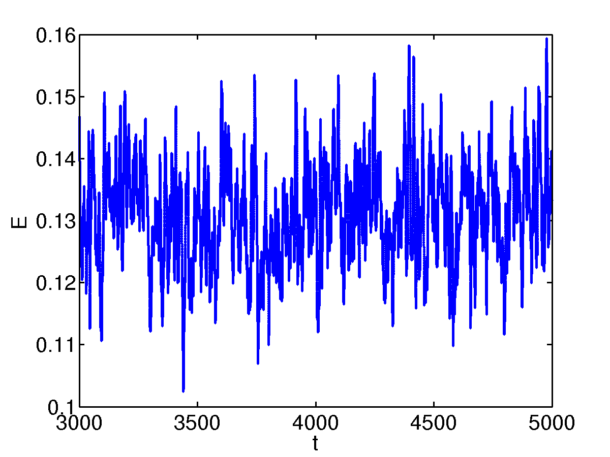
Figure 11: (Color online) Plots for $\Omega=22$ and $\mbox{Wi}=20$ : (a) the time evolution of the energy $E(t)$, (b) the power spectrum $|E(f)|$ versus the frequency $f$, and (c) the Poincaré-type section in the plane $(\Re[\hat{v}(1,0)],\Im[\hat{v}(1,0)])$. Pseudocolor plots of (d) the streamfunction $\psi$ and (e) the Okubo-Weiss parameter $\Lambda$; and (f) a filled contour plot of the reciprocal-space spectrum $E_{\Lambda}$.

III.5 Order Parameters, Spatial Correlation Functions, and Kinetic-Energy Spectra

We now use statistical measures that are employed in the density-functional theory Ramakrishnan and Yussouff (1979); Chaikin and Lubensky (2000); Oxtoby (1991); Singh (1991) of freezing. In particular, we examine the dependence of the order parameters $\langle{\hat{\Lambda}}_{\bf k}\rangle$ and the spatial autocorrelation function $G({\bf r})$, defined in Eq. (3), on Wi and $\Omega$. Recall that equilibrium melting is a first-order transition at which $\rho_{\bf G}$ jumps discontinuously from a nonzero value in the crystal to zero in the liquid. The melting of our nonequilibrium vortex crystal is far more complicated, in all parts of the parameter space of the phase diagram of Fig. 3, because there are many transitions.

For our nonequilibrium vortex crystal $\Re\langle{\hat{\Lambda}}_{\bf k}\rangle$, which is obtained by summing ${\hat{\Lambda}}_{\bf k}$ over the four forcing wave vectors, is the analog of the order parameters $\Re\langle\rho_{\bf G}\rangle$ in a conventional crystal. $\Re\langle{\hat{\Lambda}}_{\bf k}\rangle$ changes with Wi as shown, respectively, for (a) $\Omega=1$ and ${\bf k}=(4,4)$ and (b) $\Omega=22$ and ${\bf k}=(4,4)$ in Figs. 12 (a) and (b). For $\Omega=1$ and small values of Wi, the steady state of our system is SX, so the Fourier modes at the forcing wave vector are the most significant ones. As we increase Wi, our nonequilibrium system undergoes a series of transitions from SX to the turbulent state SCT (see above); therefore, $\Re\langle{\hat{\Lambda}}_{\bf k}\rangle$ decreases with Wi as we show in Fig. 12(a). For $\Omega=22$ and $\mbox{Wi}=0$, we begin with a system that is disordered and turbulent; if we then increase Wi, our system first goes to the state SX, so $\Re\langle{\hat{\Lambda}}_{\bf k}\rangle$ first increases as we show in Fig. 12(b); as we increase Wi, the system becomes turbulent and disordered again, so $\Re\langle{\hat{\Lambda}}_{\bf k}\rangle$ decreases at large Wi (Fig. 12(b)).

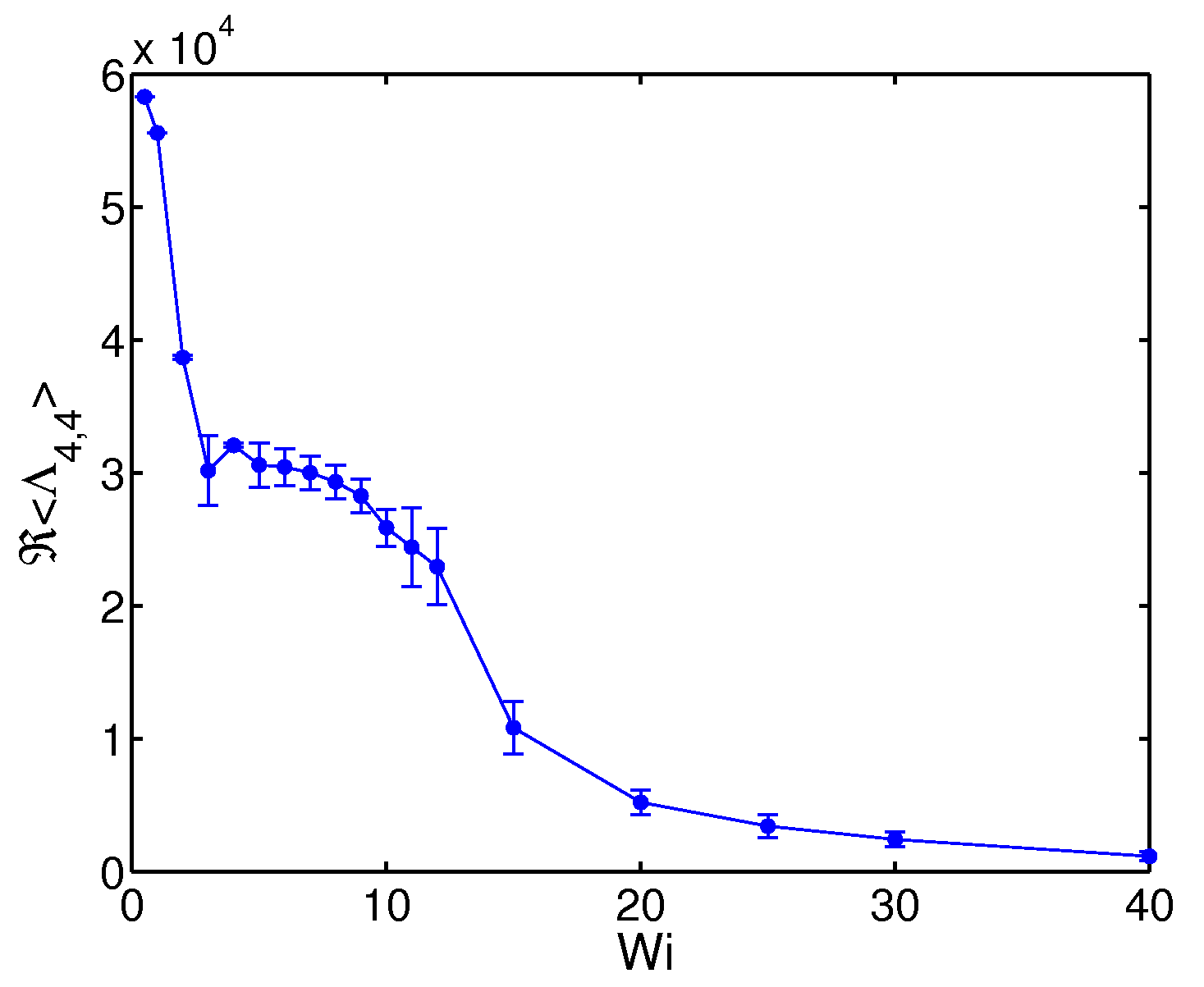
Figure 12: (Color online) Plots of $\langle{\hat{\Lambda}}_{{\bf k}=(4,4)}\rangle$ versus Wi for (a) $\Omega=1$ and for (b) $\Omega=22$; in (b) $\langle{\hat{\Lambda}}_{4,4}\rangle$ first increases with Wi, goes through a maxima, which corresponds to an OPXA state, and then decreases after that.

We give representative plots of the correlation function $G({\bf r})$ (see Eq.(3)) in Figs. 13 (a)-(d). For the crystal, we calculate $G({\bf r})$ along the line from ${\bf r}=(\pi/2,\pi/2)$ and ${\bf r}=(\pi/2,\pi)$; this shows periodic peaks [Figs. 13 (a) for $\Omega=1,\mbox{Wi}=1$] with widths that are related to those of vortical or strain-dominated regions. In the turbulent phase, we use a circular average of $G$ [Figs. 13 (b), (c), and (d) for $\Omega=1$ and $\mbox{Wi}=20$, $\Omega=22$ and $\mbox{Wi}=0$, and $\Omega=22$ and $\mbox{Wi}=20$, respectively]; these peaks decay over a length scale that yields the degree of short-range order. This decay is similar to the decay of spatial correlation functions in a disordered liquid phase in an equilibrium system. For similar, but not the same, correlation functions in a viscoelastic Taylor-Couette flow see Refs. Latrache et al. (2012, 2016).

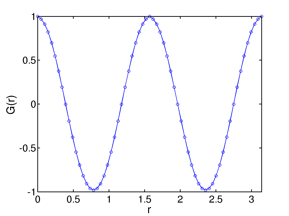
Figure 13: (Color online) (a) Plot of $G({\bf r})$ for the crystalline state with $\Omega=1$ and $\mbox{Wi}=1$ along the line connecting ${\bf r}=(\pi/2,\pi/2)$ and ${\bf r}=(\pi/2,\pi)$; and plots of the circularly averaged $G({\bf r})$ in the turbulent state with (b) $\Omega=1$ and $\mbox{Wi}=20$, (c) $\Omega=22$ and $\mbox{Wi}=0$, and (d) $\Omega=22$ and $\mbox{Wi}=20$.

We have also obtained the energy spectra $E(k)$ in two parts of the turbulent state of our system; the first part is dominated by elastic turbulence and the other one lies in the region of fluid turbulence, where polymers lead to dissipation reduction. For a given resolution, there is one qualitative difference between the energy spectra in these two regimes. In the forward-cascade part of $E(k)$, the slope of the energy spectrum is higher in the elastic-turbulence regime than in the dissipation-reduction regime as we show in Fig. 14 (a), for $\Omega=4$ and $\mbox{Wi}=10$ (red line with circles), $\Omega=4$ and $\mbox{Wi}=40$ (green line with squares), and $\Omega=50$ and $\mbox{Wi}=5$ (black line with triangles). The exponent of the energy spectra is $\simeq-3.2$, which is in reasonable agreement with the exponent in laboratory experiments of Groisman and Steinberg Groisman and Steinberg (2004). Note that, in both elastic-turbulence and dissipation-reduction regimes, the energy spectra show that the energy of the polymeric fluid is spread over many decades of $k$ (or, equivalently, over many length scales); this is a well-known signature of turbulent flows, whether they are engendered by large Re or large Wi. We have also obtained the spectrum of polymer stretching, which is defined as $[Tr(C)](k)\equiv\sum_{k-1/2<k^{\prime}\leq k+1/2}k^{\prime 2}\langle|\widehat{C_{11}}({\bf k^{\prime}},t)|^{2}+|\widehat{C_{22}}({\bf k^{\prime}},t)|^{2}\rangle_{t}$, where $\langle\rangle_{t}$ denotes the time average over the statistically steady state. In Fig. 14 (b) we show the polymer-stretching spectra, for $\Omega=4$ and $\mbox{Wi}=10$ (red line with circles), $\Omega=4$ and $\mbox{Wi}=40$ (green line with squares), and $\Omega=50$ and $\mbox{Wi}=5$ (black line with triangles).

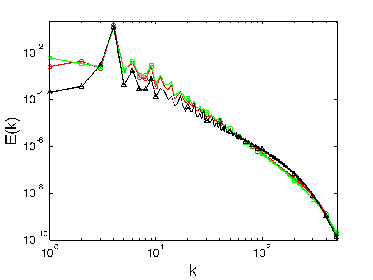
Figure 14: (Color online) Plots of (a) energy spectra $E(k)$ versus $k$ and (b) polymer stretching spectra $[{\rm Tr}{\cal C}](k)$ versus $k$, for $\Omega=4$ and $\mbox{Wi}=10$ (red line with circles), $\Omega=4$ and $\mbox{Wi}=40$ (green line with squares), and $\Omega=50$ and $\mbox{Wi}=5$ (black line with triangles).

III.6 Spatial Patterns of Polymers and Inertial Particles in the Nonequilibrium States of our System

It is instructive to study the spatial patterns of polymers and inertial particles in the nonequilibrium states of our system; we show below that such patterns also provide clear signatures of these states. In Figs. 15 (a), (b), (c), and (d) we show contours of the polymer stretching $r_{P}^{2}$ superimposed on pseudocolor plots of the Okubo-Weiss field $\Lambda$ for $\Omega=1$ and $\mbox{Wi}=1$ (crystalline state), $\Omega=1$ and $\mbox{Wi}=20$ (melted crystal in the elastic-turbulence regime), $\Omega=22$ and $\mbox{Wi}=0.5$ (frozen crystal), and $\Omega=22$ and $\mbox{Wi}=20$ (melted crystal in the dissipation-reduction regime), respectively. As we have seen in Ref Gupta et al. (2015), the polymers stretch preferentially in extensional regions, where $\Lambda<0$; thus, the patterns of their extension mirror the spatial periodicity or lack thereof in the crystalline and turbulent phases, respectively. The spatiotemporal evolution of the plots in Fig. 15 is given in Video crystal-rp-a, b, c, and d at http://www.physics.iisc.ernet.in/$\sim$rahul/movies.html .

The analogs of Figs. 15 (a), (b), (c), and (d), with polymers replaced by inertial particles (black dots), are given in Figs. 16 (a), (b), (c), and (d), respectively. We see from these plots that inertial particles organize themselves in regions where $\Lambda\simeq 0$; thus, their spatial organization can also be used to surmise the underlying periodicity of a nonequilibrium vortex crystal. This method of visualization has been used in experiments on fluid films without polymers Ouellette and Gollub (2007, 2008). All these plots are for a Stokes number ${\rm St}\simeq 1$. Note the wavy patterns of particles across the flow field, which are strongly influenced by the forcing field; these patterns are not permanent; and, as the elastic turbulence changes the particle positions, these wavy patterns of particles disappear; similar patterns appear later in time, but at different places in the simulation domain.

The analogs of Figs. 16 (a), (b), (c), and (d), with the $\Lambda$ field replaced by polymers, are given in Figs. 17 (a), (b), (c), and (d), respectively. We see from these plots that the correlation between the spatial organizations of polymers and inertial particles is not dramatic. This is not surprising insofar as the polymers stretch preferentially where $\Lambda<0$, whereas inertial particles tend to cluster in regions where $\Lambda\simeq 0$.

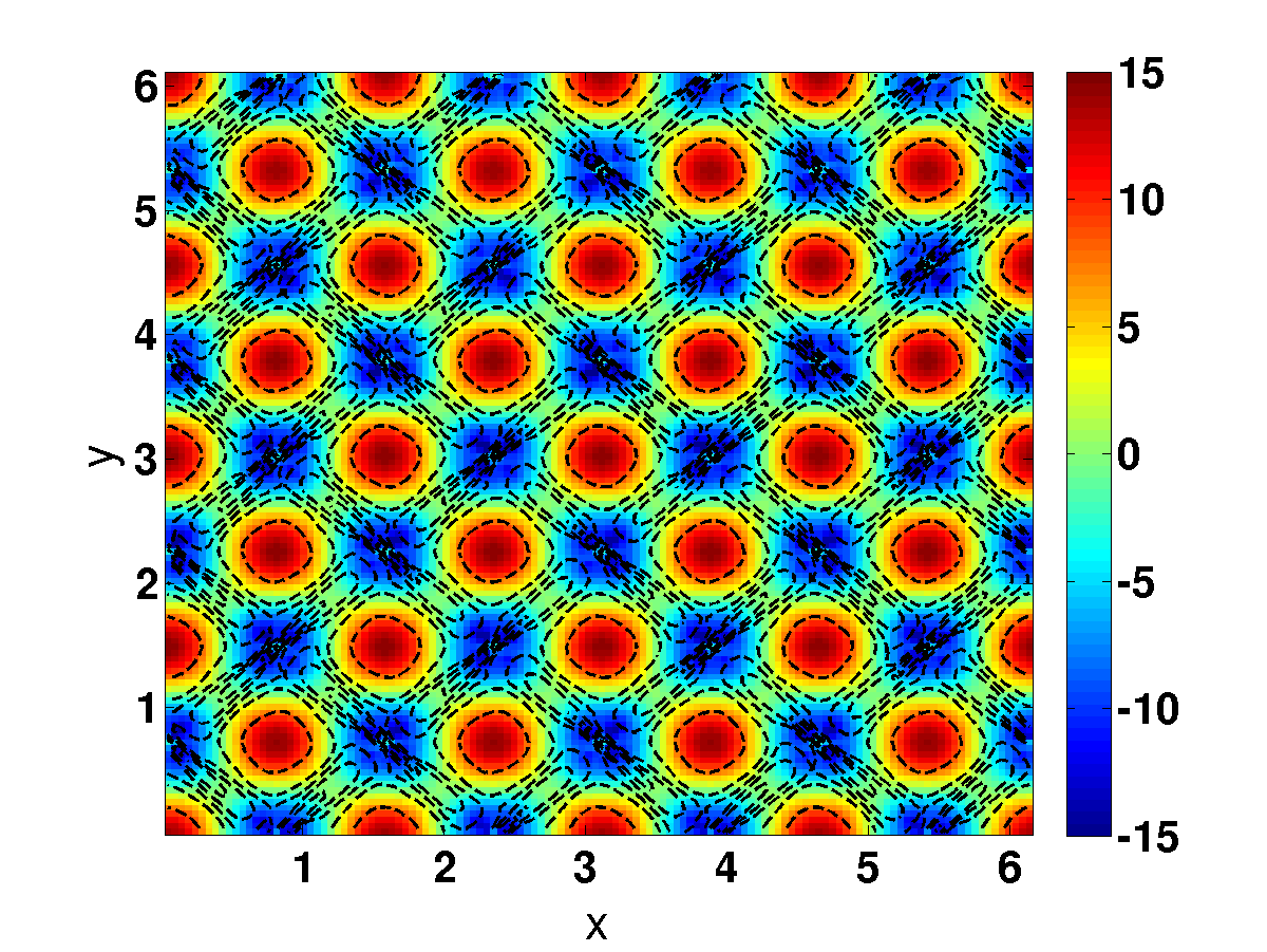
Figure 15: (Color online) Plots of contours of the polymer stretching $r_{P}^{2}$ superimposed on a pseudocolor plot of the Okubo-Weiss field $\Lambda$ for (a) $\Omega=1$ and $\mbox{Wi}=1$ (crystalline phase), (b) $\Omega=1$ and $\mbox{Wi}=20$ (melted crystal in the elastic-turbulence regime), (c) $\Omega=22$ and $\mbox{Wi}=0.5$ (frozen crystal), and (d) $\Omega=22$ and $\mbox{Wi}=20$ (melted crystal in the dissipation-reduction regime).

Figure 16: (Color online) Particle positions (black dots) superimposed on pseudocolor plots of the Okubo-Weiss field $\Lambda$ for (a) $\Omega=1$ and $\mbox{Wi}=1$ (crystalline phase), (b) $\Omega=1$ and $\mbox{Wi}=20$ (melted crystal in the elastic-turbulence regime), (c) $\Omega=22$ and $\mbox{Wi}=0.5$ (frozen crystal), and (d) $\Omega=22$ and $\mbox{Wi}=20$ (melted crystal in the dissipation-reduction regime).

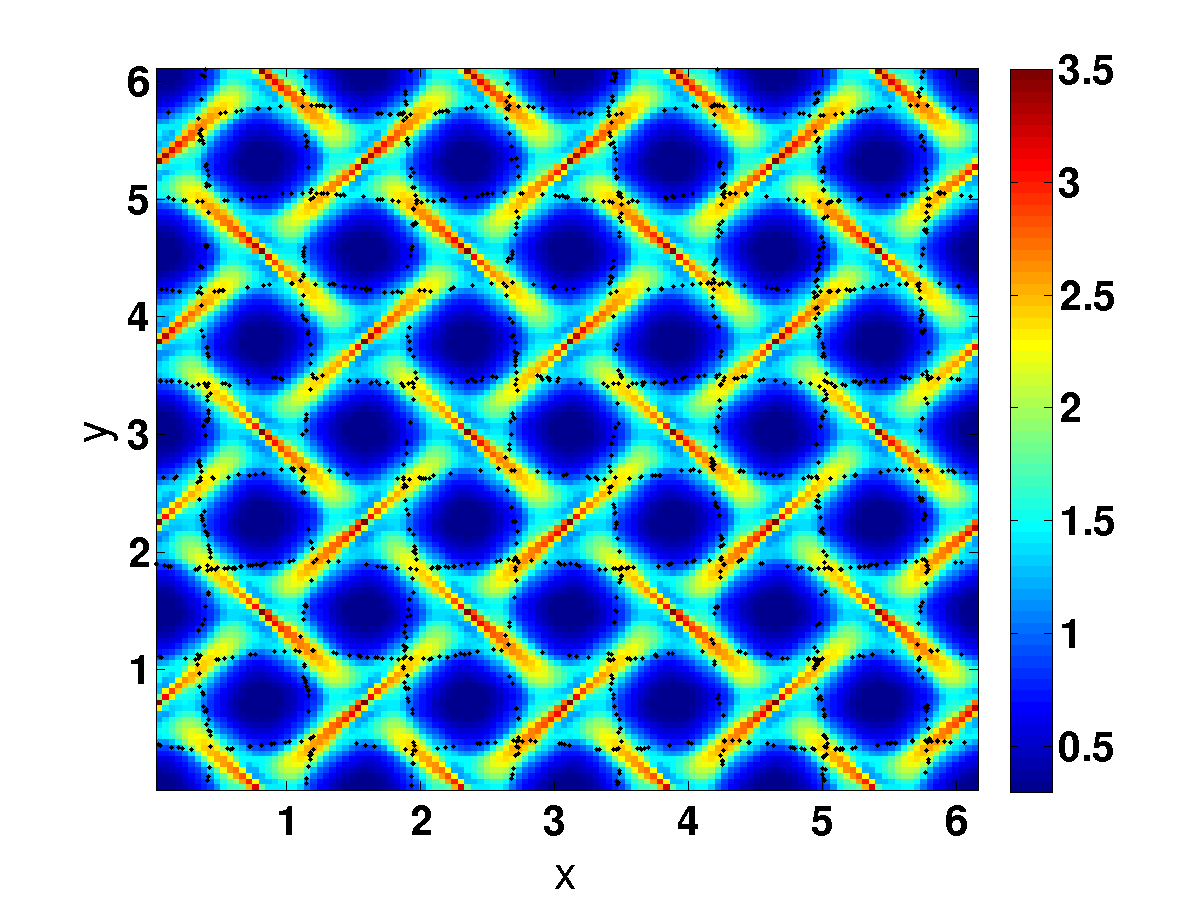
Figure 17: (Color online) Particle positions (black dots) superimposed on a pseudocolor plot of the polymer stretching $r_{P}^{2}$ for (a) $\Omega=1$ and $\mbox{Wi}=1$ (crystalline phase), (b) $\Omega=1$ and $\mbox{Wi}=20$ (melted crystal in the elastic-turbulence regime), (c) $\Omega=22$ and $\mbox{Wi}=0.5$ (frozen crystal), and (d) $\Omega=22$ and $\mbox{Wi}=20$ (melted crystal in the dissipation-reduction regime).

IV Conclusions

Our detailed DNS elucidates the nature of melting of a vortex crystal in a nonequilibrium, forced, thin fluid film with polymer additives. This melting can be induced by (a) elastic turbulence at low Reynolds numbers Re (or $\Omega$) but large Weissenberg numbers Wi (or $\tau_{P}$), (b) fluid turbulence at low Wi but large $\Omega$, or (c) a combination of these two types of turbulence (see Figs. 3 (a) and (b)). Our work leads to the rich, nonequilibrium phase diagram of Fig. 3. The topology of this phase diagram and the intricate natures of the boundaries between the different phase in it have neither been anticipated nor been studied hitherto.

Our work builds on the DNS study of Ref. Perlekar and Pandit (2010), which uses ideas from the density-functional theory of freezing Ramakrishnan and Yussouff (1979); Chaikin and Lubensky (2000); Oxtoby (1991); Singh (1991), nonlinear dynamics, and turbulence to characterize the phases and transitions in the melting, by turbulence, of a nonequilibrium vortex crystal in a 2D fluid film. Most studies of the turbulence-induced melting of a vortex crytal in a fluid film do not include polymer additives; for an overview of such studies we refer the reader to Ref. Perlekar and Pandit (2010). The DNS study of 2D fluid films with polymer additives Gupta et al. (2015); Berti et al. (2008); Berti and Boffetta (2010), which uses the Oldroyd-B model, is an exception; it has studied the elastic-turbulence-induced melting of spatially periodic Kolmogorov-flow pattern, which is, in our terminology, a one-dimensional crystal. To the best of our knowledge, there is no study of vortex crystals in fluid films with polymers, which brings together the variety of methods we use to analyze the melting of such crystals.

We follow Ref. Perlekar and Pandit (2010), which does not include polymers, in (a) identifying the order parameters for the vortex crystal, (b) characterizing the series of transitions in terms of $\psi$ and $\Lambda$, the energy time series $E(t)$, and their Fourier transforms, and (c) using the spatial correlation functions $G$ in crystalline and turbulent phases. However, we go considerably beyond the study of Ref. Perlekar and Pandit (2010) by including polymers and, therefore, (a) a new dimensionless control parameter, the Weissenberg number Wi (or $\tau_{P}$), (b) the polymer-conformation tensor field ${\mathcal{C}}$, and (c) inertial particles. Therefore, we can examine the nonequilibrium phase diagram of this system in a two-dimensional parameter space (see Figs. 3 (a) and (b)) and elucidate the organization of polymers and inertial particles in the flow, both in crystalline and turbulent phases. We show also that our system provides a natural laboratory in which we can study the crossover from elastic-turbulence to dissipation-reduction regimes in the turbulent phase.

We refer the reader to Ref. Perlekar and Pandit (2010) for a discussion of the thermodynamic limit and finite-size effects in such systems of nonequilibrium, vortex crystals. No study (including ours) has addressed these issues because, for large system sizes, we need very large DNSs to characterize the temporal evolution of the system. If we extract a correlation length from the correlation function $G$, it is much smaller than the linear size of our simulation domain in the turbulent phase (SCT), so our results should not change if we increase the system size. However, subtle size dependence might occur in the ordered phase because of the inverse cascade, well known in 2D fluid turbulence, which might lead to undulations that give rise to crystals with ever larger unit cells, whose size can be controlled only by the inclusion of friction. A systematic study of such subtle finite-size effects lies beyond the scope of our study.

The sequence of transitions that take us from a vortex crystal to the turbulent state is far richer than conventional equilibrium melting. The former differ from the latter in another important way: To maintain the steady states, statistically or strictly steady, we must impose the force $F_{\omega}$; in the language of phase transitions, this force is a symmetry-breaking field, both in the ordered and disordered phases. Therefore, there is no symmetry difference between the disordered, turbulent state and the ordered vortex crystal, as we see directly from the vestiges of the dominant peaks in the reciprocal-space spectra $E_{\Lambda}({\bf k})$; and the order parameters $\langle{\hat{\Lambda}}_{\bf k}\rangle$, with ${\bf k}=(4,4)$ the forcing wave vectors, do not become exactly zero in the turbulent phase; however, they do become very small. Moreover, our nonequilibrium vortex crystal undergoes a sequence of transitions from an ordered state to an undulating crystal and then to a fully turbulent state; there is no external or thermal noise here and hence no fluctuations in the perfect vortex crystal; this has no equilibrium analog.

We hope that our study will encourage experimental groups to try to obtain the rich phase diagram of the melting of a nonequilibrium vortex crystal in a fluid film with polymer additives. In particular, experiments on such a system could look for spatiotemporal crystals, which are periodic both in space and time and which cannot be obtained easily in nonequilibrium, hard-matter settings. Furthermore, the reentrant crystallization, i.e., the recrystallization, with an increase in Wi, of the melted crystal, which emerges from our detailed DNS, is certainly worth exploring in experiments. We have recently learnt of a shell-model study of elastic turbulence that is just published Ray and Vincenzi (2016).

V Acknowledgments

We thank the Council for Scientific and Industrial Research, University Grants Commission, and Department of Science and Technology (India) for support, SERC (IISc) for computational resources, and P.Perlekar, D. Mitra, S.S. Ray, and D. Vincenzi for discussions. AG acknowledges gratefully funding from the European Research Council under the European Community’s Seventh Framework Programme (FP7/2007-2013)/ERC Grant Agreement N. 279004.

References

References

- Ramakrishnan and Yussouff (1979) T. V. Ramakrishnan and M. Yussouff, Physical Review B 19, 2775 (1979).
- Haymet (1987) A. Haymet, Annual Review of Physical Chemistry 38, 89 (1987).
- Chaikin and Lubensky (2000) P. M. Chaikin and T. C. Lubensky, Principles of condensed matter physics, vol. 1 (Cambridge Univ Press, 2000).
- Oxtoby (1991) D. Oxtoby, Les Houches Summer School Lectures vol LI (1991).
- Singh (1991) Y. Singh, Physics Reports 207, 351 (1991).
- Perlekar and Pandit (2010) P. Perlekar and R. Pandit, New Journal of Physics 12, 023033 (2010).
- Das et al. (2002) M. Das, S. Ramaswamy, and G. Ananthakrishna, EPL (Europhysics Letters) 60, 636 (2002).
- Gotoh and Yamada (1984) K. Gotoh and M. Yamada, Physical Society of Japan, Journal 53, 3395 (1984).
- Gotoh and Yamada (1987) K. Gotoh and M. Yamada, Fluid dynamics research 1, 165 (1987).
- Doering and Gibbon (1995) C. R. Doering and J. D. Gibbon, Applied analysis of the Navier-Stokes equations, vol. 12 (Cambridge University Press, 1995).
- Ouellette and Gollub (2007) N. T. Ouellette and J. P. Gollub, Physical Review Letters 99, 194502 (2007).
- Ouellette and Gollub (2008) N. T. Ouellette and J. P. Gollub, Physics of Fluids 20, 064104 (2008).
- Perlekar et al. (2010) P. Perlekar, D. Mitra, and R. Pandit, Physical Review E 82, 066313 (2010).
- Perlekar et al. (2006) P. Perlekar, D. Mitra, and R. Pandit, Physical Review Letters 97, 264501 (2006).
- Gupta et al. (2015) A. Gupta, P. Perlekar, and R. Pandit, Phys. Rev. E 91, 033013 (2015).
- Groisman and Steinberg (2000) A. Groisman and V. Steinberg, Nature 405, 53 (2000).
- Groisman and Steinberg (2001) A. Groisman and V. Steinberg, Nature 410, 905 (2001).
- Ganapathy and Sood (2006) R. Ganapathy and A. K. Sood, Physical review letters 96, 108301 (2006).
- Majumdar and Sood (2011) S. Majumdar and A. K. Sood, Physical Review E 84, 015302 (2011).
- Braun et al. (1997) R. Braun, F. Feudel, and N. Seehafer, Physical Review E 55, 6979 (1997).
- Molenaar et al. (2007) D. Molenaar, H. J. H. Clercx, G. J. F. van Heijst, and Z. Yin, Physical Review E 75, 036309 (2007).
- Berti et al. (2008) S. Berti, A. Bistagnino, G. Boffetta, A. Celani, and S. Musacchio, Physical Review E 77, 055306 (2008).
- Berti and Boffetta (2010) S. Berti and G. Boffetta, Physical Review E 82, 036314 (2010).
- Chomaz and Cathalau (1990) J. M. Chomaz and B. Cathalau, Physical Review A 41, 2243 (1990).
- Chomaz (2001) J. Chomaz, Journal of Fluid Mechanics 442, 387 (2001).
- Perlekar and Pandit (2009) P. Perlekar and R. Pandit, New Journal of Physics 11, 073003 (2009).
- Okubo (1970) A. Okubo, in Deep Sea Research and Oceanographic Abstracts (Elsevier, 1970), vol. 17, pp. 445–454.
- Weiss (1991) J. Weiss, Physica D: Nonlinear Phenomena 48, 273 (1991).
- Rivera et al. (2001) M. Rivera, X.-L. Wu, and C. Yeung, Physical Review Letters 87, 044501 (2001).
- Elhmaïdi et al. (1993) D. Elhmaïdi, A. Provenzale, and A. Babiano, Journal of Fluid Mechanics 257, 533 (1993).
- Platt et al. (1991) N. Platt, L. Sirovich, and N. Fitzmaurice, Physics of Fluids A 3, 681 (1991).
- Kurganov and Tadmor (2000) A. Kurganov and E. Tadmor, Journal of Computational Physics 160, 241 (2000).
- Frigo and Johnson (1999) M. Frigo and S. G. Johnson, Massachusetts Institute of Technology (1999).
- Vaithianathan and Collins (2003) T. Vaithianathan and L. R. Collins, Journal of Computational Physics 187, 1 (2003).
- Maxey and Riley (1983) M. R. Maxey and J. J. Riley, Physics of fluids 26, 883 (1983).
- Gatignol (1983) R. Gatignol, J. Mec. Theor. Appl 1, 143 (1983).
- Bec et al. (2006) J. Bec, L. Biferale, G. Boffetta, A. Celani, M. Cencini, A. Lanotte, S. Musacchio, and F. Toschi, Journal of Fluid Mechanics 550, 10 (2006).
- Boffetta et al. (2004) G. Boffetta, F. De Lillo, and A. Gamba, Physics of Fluids 16, L20 (2004).
- De Lillo et al. (2012) F. De Lillo, G. Boffetta, and S. Musacchio, Physical Review E 85, 036308 (2012).
- Schneider et al. (2007) T. M. Schneider, B. Eckhardt, and J. A. Yorke, Physical review letters 99, 034502 (2007).
- Shajahan et al. (2007) T. K. Shajahan, S. Sinha, and R. Pandit, Physical Review E 75, 011929 (2007).
- Shajahan et al. (2009) T. K. Shajahan, A. R. Nayak, and R. Pandit, PloS one 4, e4738 (2009).
- Sahoo et al. (2010) G. Sahoo, D. Mitra, and R. Pandit, Physical Review E 81, 036317 (2010).
- Latrache et al. (2012) N. Latrache, O. Crumeyrolle, and I. Mutabazi, Physical Review E 86, 056305 (2012).
- Latrache et al. (2016) N. Latrache, N. Abcha, O. Crumeyrolle, and I. Mutabazi, Physical Review E 93, 043126 (2016).
- Groisman and Steinberg (2004) A. Groisman and V. Steinberg, New Journal of Physics 6, 29 (2004).
- Ray and Vincenzi (2016) S. S. Ray and D. Vincenzi, Europhys. Lett. 114, 44001 (2016).