Efficient Bayesian Inference for Multivariate Factor Stochastic Volatility Models

Abstract

We discuss efficient Bayesian estimation of dynamic covariance matrices in multivariate time series through a factor stochastic volatility model. In particular, we propose two interweaving strategies (Yu and Meng, 2011) to substantially accelerate convergence and mixing of standard MCMC approaches. Similar to marginal data augmentation techniques, the proposed acceleration procedures exploit non-identifiability issues which frequently arise in factor models. Our new interweaving strategies are easy to implement and come at almost no extra computational cost; nevertheless, they can boost estimation efficiency by several orders of magnitude as is shown in extensive simulation studies. To conclude, the application of our algorithm to a 26-dimensional exchange rate data set illustrates the superior performance of the new approach for real-world data.

Abstract

This document contains supplementary material for the paper “Efficient Bayesian Inference for Multivariate Factor Stochastic Volatility Models”. It encloses (A.1) details of the various sampling steps of Algorithm 1 and details concerning the R package factorstochvol, (A.2) the data generating parameter values for the simulation study in Section 4, and (A.3) further results for the exchange rate data discussed in Section 5.

Forthcoming in:
Journal of Computational and Graphical Statistics
doi:10.1080/10618600.2017.1322091

Keywords: Ancillarity-sufficiency interweaving strategy (ASIS), Curse of dimensionality, Data augmentation, Dynamic correlation, Dynamic covariance, Exchange rate data, Markov chain Monte Carlo (MCMC)

1 Introduction

The analysis of multivariate time series has become a vivid research area over the last decades, where both methodological as well as computational advances have made it possible to estimate more and more complex models. In parallel, real-world applications with an ever-increasing amount of data call for the joint modeling of many simultaneous and often co-varying observations over time. However, already the number of pair-wise co-movements increases quadratically with the number of time series, let alone higher-dimensional dependency structures. This property, often referred to as the curse of dimensionality, can often be mitigated in various ways by imposing a lower-dimensional latent factor structure, thereby effectively reducing the number of parameters to a feasible amount. In the paper at hand, we particularly focus on the case where these factors are allowed to have time-varying variances which in turn drive the multivariate dynamics. To the best of our knowledge, models of this type have first been discussed by Jacquier et al. (1994), Shephard (1996), and Kim et al. (1998). We particularly focus on the model formulation brought forward by Chib et al. (2006).

Applications of multivariate factor stochastic volatility models typically reside in the field of financial econometrics, most prominently in areas that involve accurate quantification of uncertainty and risk. Examples thereof are asset allocation (e.g. Aguilar and West, 2000; Han, 2006; Zhou et al., 2014) and asset pricing (e.g. Nardari and Scruggs, 2007). These models extend standard factor pricing models such as the arbitrage pricing theory (Ross, 1976) and the capital asset pricing model (Sharpe, 1964; Lintner, 1965) by relaxing the assumption that the multivariate volatility dynamics are constant over time.

Statistical estimation of these models can be challenging, and a variety of solutions such as quasi-maximum likelihood (e.g. Harvey et al., 1994) or simulated maximum likelihood (e.g. Liesenfeld and Richard, 2006; Jungbacker and Koopman, 2006) have been proposed. For medium to high dimensional problems, Bayesian MCMC estimation (Pitt and Shephard, 1999; Aguilar and West, 2000; Chib et al., 2006; Han, 2006; Omori et al., 2007) is probably the most efficient estimation method, however, it is associated with a considerable computational burden when the number of assets is moderate to large.

The aim of this work is to outline a reliable method for Bayesian inference that performs well for a wide range of data sets while at the same time being easy to implement and convenient to extend. Therefore, we combine an efficient method for estimating univariate stochastic volatility models introduced by Kastner and Frühwirth-Schnatter (2014) with a standard Gibbs sampler for regression problems. To ensure fast convergence and proper mixing of the MCMC chains we augment this simple procedure with interweaving strategies introduced by Yu and Meng (2011). Through extensive simulation studies and a real-world example, we demonstrate the effectiveness of our procedure which can boost sampling efficiency by a factor of 100 and more.

The remainder of this paper is structured as follows. Section 2 establishes notation for the factor stochastic volatility model framework and discusses questions about model specification and identification. Section 3 gives an in-depth exposure to the estimation algorithm and its implementation, whereby the focus is placed on the novel interweaving strategies employed. Section 4 presents measures of sampling efficiency for simulated data sets and compares the algorithms presented. Section 5 discusses a case study with $26$ daily EUR exchange rates. Section 6 concludes.

2 The Multivariate Factor Stochastic Volatility Model

In a multivariate framework, the quadratic growth of the number of covariances alongside their inherent time-variability calls for a model which is sufficiently parsimoniously specified. At the same time, the model needs to be flexible enough to have the potential to capture typical features of financial and economic time series such as volatility clustering and volatility co-movement. On top of that, common irregularities in the data require the model to be robust with respect to idiosyncratic shocks.

The multivariate factor stochastic volatility (SV) model (Chib et al., 2006) aims at uniting simplicity with flexibility and robustness. It is simple in the sense that the potentially high-dimensional observation space is reduced to a lower-dimensional orthogonal latent factor space, just like in the case of the classic factor model. It is flexible in the sense that these factors are allowed to exhibit volatility clustering, and it is robust in the sense that idiosyncratic deviations are themselves stochastic volatility processes, thereby allowing for the degree of volatility co-movement to be time-varying.

2.1 Model Specification

For each point in time $t=1,\ldots,T$, let ${\bm{y}}_{t}=(y_{1t},\ldots,y_{mt})^{{}^{\prime}}$ be a zero-mean vector of $m$ observed returns and let ${\bm{f}}_{t}=(f_{1t},\ldots,f_{rt})^{{}^{\prime}}$ be a vector of $r$ unobserved latent factors. In analogy to the static factor model, the observations are assumed to be driven by the latent factors and the idiosyncratic innovations. In the case of the factor stochastic volatility model, however, both the idiosyncratic innovations as well as the latent factors are allowed to have time-varying variances, depending on $m+r$ latent volatilities ${\bm{h}}_{t}=({\bm{h}}_{t}^{U},{\bm{h}}_{t}^{V})$, where ${\bm{h}}_{t}^{U}=(h_{1t},\ldots,h_{mt})^{{}^{\prime}}$ and ${\bm{h}}_{t}^{V}=(h_{m+1,t},\ldots,h_{m+r,t})^{{}^{\prime}}$. In short, we have

$${\bm{y}}_{t}=\bm{\Lambda}{\bm{f}}_{t}+{\bm{{{U}}}}_{t}({\bm{h}}_{t}^{U})^{1/2}\bm{\epsilon}_{t},\qquad{\bm{f}}_{t}={\bm{V}}_{t}({\bm{h}}^{V}_{t})^{1/2}\bm{\zeta}_{t},$$ (1)

where $\bm{\Lambda}$ is an unknown $m\times r$ factor loadings matrix, ${\bm{{{U}}}}_{t}({\bm{h}}^{U}_{t})=\mbox{\text{d}iag}\!\left(\exp(h_{1t}),\ldots,\exp(h_{mt})\right)$ is a diagonal $m\times m$ matrix containing the idiosyncratic (series-specific) variances, and ${\bm{V}}_{t}({\bm{h}}^{V}_{t})=\mbox{\text{d}iag}\!\left(\exp(h_{m+1,t}),\ldots,\exp(h_{m+r,t})\right)$ is a diagonal $r\times r$ matrix containing the factor variances. These variances are themselves modeled as latent variables whose logarithms follow independent autoregressive processes of order one, i.e. for $i=1,\ldots,m+r$:

$$h_{it} = \mu_{i}+\phi_{i}(h_{i,t-1}-\mu_{i})+\sigma_{i}\eta_{it},$$ (2)

with unknown initial value $h_{i0}$.

All innovations are assumed to follow independent standard normal distributions, i.e. $\bm{\epsilon}_{t}\sim\mathcal{N}_{m}\!\left({\bm{{0}}},{{\bm{I}}}_{m}\right)$, $\bm{\zeta}_{t}\sim\mathcal{N}_{r}\!\left({\bm{{0}}},{{\bm{I}}}_{r}\right)$, and $\bm{\eta}_{t}\sim\mathcal{N}_{m+r}\!\left({\bm{{0}}},{{\bm{I}}}_{m+r}\right)$, where $\bm{\eta}_{t}=(\eta_{1t},\dots,\eta_{m+r,t})^{\prime}$. This implies following structure:

$${\bm{y}}_{t}=\bm{\Lambda}{\bm{f}}_{t}+\bm{\varepsilon}_{t},\qquad{\bm{f}}_{t}|{\bm{h}}_{t}\sim\mathcal{N}_{r}\!\left({\bm{{0}}},{\bm{V}}_{t}({\bm{h}}^{V}_{t})\right),$$ (3)

with $\bm{\varepsilon}_{t}|{\bm{h}}_{t}\sim\mathcal{N}_{m}\!\left({\bm{{0}}},{\bm{{{U}}}}_{t}({\bm{h}}_{t})\right)$. One of the main reasons for estimating a factor SV model is to reliably estimate the potentially time-varying conditional covariance matrix of ${\bm{y}}_{t}$ which, for the model at hand, is given by $\text{cov}({\bm{y}}_{t}|{\bm{h}}_{t})={\bm{\Sigma}}_{t}({\bm{h}}_{t})=\bm{\Lambda}{\bm{V}}_{t}({\bm{h}}^{V}_{t})\bm{\Lambda}^{\prime}+{\bm{{{U}}}}_{t}({\bm{h}}^{U}_{t})$. Note that because ${\bm{{{U}}}}_{t}({\bm{h}}^{U}_{t})$ is diagonal, all covariances between the component series are governed by the latent factors. Marginally with respect to ${\bm{h}}_{t}$, ${\bm{y}}_{t}$ is a process with non-Gaussian stationary distribution.

2.2 Identification Issues

Whenever certain combinations of parameter values result in (almost) identical maxima in the likelihood function, estimation of the corresponding parameter values from data can become impossible. Consequently, observationally equivalent parameter constellations must be ruled out for reliable statistical inference and a large body of literature dealing with this issue has arisen. In particular, Frühwirth-Schnatter and Lopes (2017) give an overview of recent advances in the context of static Bayesian factor models, and Sentana and Fiorentini (2001) specifically discuss identification for models where the factors exhibit conditional heteroscedasticity (but innovations are assumed to be homoscedastic). If not dealt with properly, usually through certain restrictions on the parameter space, sensible interpretation of the posterior distribution is not possible (“nonidentifiability”). In less severe cases (“near-nonidentifiability”), MCMC algorithms and other estimation procedures often lack convergence and thus provide unreliable results. For the model at hand, we face several issues related to this problem.

First, to prevent factor rotation and column switching, one option is to follow the usual convention and set the upper triangular part of $\bm{\Lambda}$ to zero and $\mbox{\text{d}iag}\!\left(\bm{\Lambda}\right)$ nonzero (e.g. Geweke and Zhou, 1996). Doing so, however, imposes an – often unwanted – order dependence. We therefore also discuss the possibility to leave the factor loadings matrix unrestricted and deal with column switching through post-processing of the MCMC draws.

Second, without identifying the scaling of either the $j$th column of $\bm{\Lambda}$ or the variance of $f_{jt}$, the model is not identified. The usual remedy (e.g. Aguilar and West, 2000; Chib et al., 2006; Han, 2006; Lopes and Carvalho, 2007; Nakajima and West, 2013; Zhou et al., 2014) is that the diagonal loading elements in model (3) are fixed to one, i.e. $\Lambda_{jj}=1$, for $j=1,\ldots,r$, while the level $\mu_{m+j}$ of the factor volatilities $h_{m+j,t}$ in model (2) (which corresponds to the scaling of $f_{jt}$) is modeled to be unknown. This approach implies that the first $r$ variables are leading the factors and thus makes variable ordering an even more important modeling decision. To alleviate this issue, we leave the diagonal elements $\Lambda_{jj}$ in model (3) unrestricted, an intuitive interpretation being that “leadership” of a factor can be shared by several series. Instead, we fix the level $\mu_{m+j}$ of the factor volatilities $h_{m+j,t}$ at zero:

$$h_{it}=(1-\phi_{i})\mu_{i}+\phi_{i}h_{i,t-1}+\sigma_{i}\eta_{it},\quad i=1,\ldots,m,$$

$$h_{m+j,t}=\phi_{m+j}h_{m+j,t-1}+\sigma_{m+j}\eta_{m+j,t},\quad j=1,\ldots,r.$$ (4)

This assumption, alongside the prior distribution on the loadings introduced in Section 3.1, identifies the factor variance.

Finally, each column of $\bm{\Lambda}$ is only identified up to a possible sign switch. We deal with this (lightweight) identification issue a posteriori, meaning that we run our MCMC sampler in the unrestricted model and identify signs afterwards, see Section A.1.4 in Appendix A.1 for details.

Factor model (3) together with the $m+r$ SV models (4) defines our baseline parameterization, however alternative parameterizations will be exploited in Section 3.3 in the context of efficient MCMC estimation of the factor SV model.

3 Bayesian Inference

We perform Bayesian inference based on a set of carefully selected proper priors which are introduced in Section 3.1 and develop efficient schemes for full conditional MCMC sampling in the remaining subsections.

3.1 Prior Distributions

Independently for each $i\in\{1,\dots,m+r\}$, priors for the univariate SV processes are chosen as in Kastner and Frühwirth-Schnatter (2014): $p(\mu_{i},\phi_{i},\sigma_{i})$ = $p(\mu_{i})p(\phi_{i})p(\sigma_{i})$, where the level $\mu_{i}\in\mathbb{R}$ is equipped with the usual normal prior $\mu_{i}\sim\mathcal{N}\!\left(b_{\mu},B_{\mu}\right)$, the persistence parameter $\phi_{i}\in(-1,1)$ is chosen according to $(\phi_{i}+1)/2\sim\mathcal{B}\!\left(a_{0},b_{0}\right)$ as in Kim et al. (1998), and the volatility of log variance $\sigma_{i}\in\mathbb{R}^{+}$ is implied by $\sigma_{i}^{2}\sim B_{\sigma}\times\chi^{2}_{1}=\mathcal{G}\!\left(\frac{1}{2},\frac{1}{2B_{\sigma}}\right)$. The initial state $h_{i0}$ is distributed according to the stationary distribution of the AR($1$) process (2), i.e. $h_{i0}|\mu_{i},\phi_{i},\sigma_{i}\sim\mathcal{N}\!\left(\mu_{i},\sigma_{i}^{2}/(1-\phi_{i}^{2})\right)$. For every unrestricted element of the factor loadings matrix we choose independent zero-mean Gaussian distributions, i.e. $\Lambda_{ij}\sim\mathcal{N}\!\left(0,B_{\Lambda}\right)$.

3.2 Full Conditional MCMC estimation

Bayesian inference operates directly in the latent variable model (3) and (4) and relies on data augmentation by introducing the latent volatilities ${\bm{h}}=\{{\bm{h}}_{i,\bullet}\},i=1,\ldots,m+r$, where ${\bm{h}}_{i,\bullet}=(h_{i0},h_{i1},\dots,h_{iT})^{\prime}$, and the latent factors ${\bm{f}}=\{{\bm{f}}_{j,\bullet}\},j=1,\ldots,r$, where ${\bm{f}}_{j,\bullet}=(f_{j1},\dots,f_{jT})^{\prime}$, as latent data. This allows to set up a simple scheme for full conditional MCMC sampling which is outlined in Algorithm 1 and discussed in detail thereafter.

Algorithm 1.

Choose appropriate starting values for $\mu_{i}$, $i\in\{1,\dots,m\}$, $\phi_{i}$ and $\sigma_{i}$, $i\in\{1,\dots,m+r\}$, as well as $\bm{\Lambda}$, ${\bm{h}}$ and ${\bm{f}}$ and repeat the following steps:

1. Perform in total $m+r$ univariate SV updates of the $m$ idiosyncratic variances ${\bm{h}}_{i,\bullet}$ as well as the parameters $(\mu_{i},\phi_{i},\sigma_{i})$, independently for each $i=1,\dots,m$, and of the $r$ factor variances ${\bm{h}}_{m+j,\bullet}$ as well as the parameters $(\phi_{m+j},\sigma_{m+j})$, independently for each $j=1,\dots,r$.

2. For $i=1,\dots,m$, sample each row $\bm{\Lambda}_{i,\bullet}$ of the factor loading matrix from $\bm{\Lambda}_{i,\bullet}|{\bm{f}},{\bm{y}}_{i,\bullet},{\bm{h}}_{i,\bullet}$. This step constitutes $m$ independent $\tilde{r}_{i}$-variate regression problems with $T$ observations, where $\tilde{r}_{i}$ denotes the number of unrestricted elements in $\bm{\Lambda}_{i,\bullet}$.

3. Redraw the diagonal elements of $\bm{\Lambda}$ through interweaving into the state equation for the latent factors (shallow interweaving) or through interweaving into the state equation for the latent volatilities (deep interweaving).

4. For $t=1,\dots,T$, sample ${\bm{f}}_{t}$ from ${\bm{f}}_{t}|\bm{\Lambda},{\bm{y}}_{t},{\bm{h}}_{t}$, constituting $T$ independent $r$-variate regression problems with $m$ observations.

For Step (a), observe that conditional on knowing the latent factors ${\bm{f}}$ and the loadings $\bm{\Lambda}$, we are dealing with $m+r$ independent, univariate SV models where the latent state equations (4) are combined with following observation equations:

$$\log(y_{it}-\bm{\Lambda}_{i,\bullet}{\bm{f}}_{t})^{2} = h_{it}+\log\epsilon_{it}^{2},\qquad i=1,\ldots,m,$$ (5)

$$\log f_{jt}^{2} = h_{m+j,t}+\log\zeta_{jt}^{2},\qquad j=1,\ldots,r.$$ (6)

Hence, sampling the latent volatilities ${\bm{h}}_{i,\bullet}$ as well as the parameters $(\mu_{i},\phi_{i},\sigma_{i})$ for $i=1,\ldots,m+r$ (with $\mu_{i}=0$ for $i>m$) in Step (a) amounts to $m+r$ univariate SV updates. Consequently, the substantial amount of research on this matter which has emerged in the last two decades can directly be applied. In particular, we follow recent findings in Kastner and Frühwirth-Schnatter (2014), where an efficient sampling scheme is proposed and evaluated, and simply use the implementation in the R package stochvol (Kastner, 2016a) as a “plug-in” for Step (a) of the factor SV sampler presented in Algorithm 1; see Appendix A.1.1 for more details and additional references on MCMC estimation for univariate SV models.

On the other hand, conditional on knowing the latent volatilities ${\bm{h}}$, we are dealing in (3) with a factor model with heteroscedastic errors. Nevertheless, given ${\bm{h}}$, ${\bm{f}}$ and $\bm{\Lambda}$ may be sampled conditionally on each other from the respective multivariate normal distributions in a similar manner as for a standard factor model (Lopes and West, 2004). This approach is conceptually straightforward, see Appendix A.1.2 for details how to sample in Step (b) each row $\bm{\Lambda}_{i,\bullet}$ of the factor loading matrix from $\bm{\Lambda}_{i,\bullet}|{\bm{f}},{\bm{y}}_{i,\bullet},{\bm{h}}_{i,\bullet}$, where ${\bm{y}}_{i,\bullet}=(y_{i1},\ldots,y_{iT})^{\prime}$, and Appendix A.1.3 for details how to sample in Step (c) the factor ${\bm{f}}_{t}$ from ${\bm{f}}_{t}|\bm{\Lambda},{\bm{y}}_{t},{\bm{h}}_{t}$ for $t=1,\dots,T$.

After discarding a certain amount of initial draws (the burn-in), the standard full conditional sampler iterates steps (a), (b) and (c) of Algorithm 1, but not (b*), and should, in principle, yield draws from the joint posterior distribution. However, when estimating factor SV models through such an MCMC scheme, slow convergence and poor mixing (i.e. high correlation of posterior draws) can become a potentially prohibitive issue. This phenomenon substantiates in enormous autocorrelation of posterior draws – even after thinning – and can render MCMC output practically useless. For certain data sets, the burn-in phase may take extremely long and a huge amount of samples has to be discarded before the draws can be considered to emerge from the posterior distribution. Additionally, even after burn-in, these draws often show extraordinarily high autocorrelation and thus only explore the target distribution painstakingly slowly. These so-called badly mixing samplers do not only prolong computation time, they also frequently lead to unreliable estimates and misleading results. The simulation study in Section 4 illustrates that this can happen for the standard full conditional sampler even with data simulated from the true model, see e.g. the top of the two panels in Figure 1. Consequently, a carefully crafted posterior simulator is of utmost importance.

To overcome this problem, Chib et al. (2006) propose to sample the factor loading matrix $\bm{\Lambda}$ from the marginalized conditional posterior $p(\bm{\Lambda}|{\bm{y}},{\bm{h}})$, without conditioning on the factors ${\bm{f}}$. This distribution, however, is not available in closed form, and to sample from it requires a rather involved Metropolis-Hastings update where the proposal distribution is based on numerically maximizing the often high-dimensional conditional likelihood function and approximating its Hessian matrix at every MCMC iteration. To avoid this potential bottleneck, we employ the simpler full conditional procedure outlined in Algorithm 1 but enhance it in Step (b*) by employing two variants of an ancillarity-sufficiency interweaving strategy (ASIS) (Yu and Meng, 2011), called shallow interweaving and deep interweaving, which are explained in detail in Section 3.3.

Applications to simulated data in Section 4 as well as to exchange rate data in Section 5 illustrate how adding Step (b*) boosts MCMC dramatically, in particular for deep interweaving; compare e.g. the top panel in Figure 1 to the remaining panels. Section A.1.5 in Appendix A.1 provides comments on practical implementation of the boosted Algorithm 1 using the R package factorstochvol (Kastner, 2016b).

3.3 Boosting Full Conditional MCMC through Interweaving

As discussed in Section 3.2, the standard full conditional sampler outlined in Algorithm 1 is based on data augmentation in the parameterization (3) and (4) of the factor SV model and suffers from slow convergence like so many other MCMC schemes which alternate between sampling from the full conditionals of the latent states and the model parameters. A large literature has emerged discussing various techniques to improve such algorithms, in particular reparameterization (Papaspiliopoulos et al., 2007), marginal data augmentation (van Dyk and Meng, 2001), and interweaving strategies (Yu and Meng, 2011).

Reparameterization relies on data augmentation in a different parameterization of the model with alternative latent variables. In particular, so-called non-centered parameterizations where unknown model parameters are moved from the latent state equation to the observation equation proved to be useful, see e.g. Frühwirth-Schnatter and Wagner (2010) in the context of state space modeling of time series. However, MCMC estimation based on different data augmentation schemes will often be efficient in separate regions of the parameter space, as demonstrated e.g. by Kastner and Frühwirth-Schnatter (2014) in the context of univariate SV models. This suggests to combine different data augmentation schemes to obtain an improved sampler.

Marginal data augmentation employs a randomly sampled “working parameter” to transform the baseline parameterization to an expanded, unidentified latent variable model in which the model parameters are updated conditional on the (randomly) transformed latent variables. This technique has been applied to the basic factor model, using the undefined scaling of the factors as a working parameter (Ghosh and Dunson, 2009; Frühwirth-Schnatter and Lopes, 2017), however, it is not easily extended to factor SV models, in particular if the latent volatilities should be part of the acceleration scheme.

The ancillarity-sufficiency interweaving strategy (ASIS), introduced by Yu and Meng (2011), provides another principled way to interweave two different data augmentation schemes by re-sampling certain parameters conditional on the latent variables in an alternative parameterization of the model, thereby combining “best of different worlds”. ASIS has been successfully employed in a variety of contexts such as univariate SV models (Kastner and Frühwirth-Schnatter, 2014) and dynamic linear state space models (Simpson, 2015; Simpson et al., 2017). To boost Algorithm 1, we apply ASIS to the factor SV model in the present paper. Two interweaving strategies – called shallow interweaving and deep interweaving – are derived in Section 3.3.1, where the diagonal elements $\Lambda_{11},\ldots,\Lambda_{rr}$ of the factor loadings matrix are resampled in Step (b*) in two alternative parameterizations of the model.

As will become clear in the following sections, deep interweaving typically yields the highest sampling efficiency gains and is thus the generally recommended strategy. However, also shallow interweaving has its merits. First, being conditionally conjugate, it is somewhat easier to implement. Second, it can be applied also to static factor models which are by construction not suited for deep interweaving (see also Bitto and Frühwirth-Schnatter, 2016).

3.3.1 Shallow and Deep Interweaving

As discussed in Section 2.2, our baseline parameterization (3) and (4) is just one of several alternative ways to handle the scaling problem inherent in factor SV models and this identification issue is exploited by our schemes.

The parameterization underlying shallow interweaving constrains the diagonal elements of the factor loadings matrix to be equal to 1, whereas the variances of the factors depend on $r$ unknown scaling parameters ${\bm{D}}=\mbox{\text{d}iag}\!\left(\Lambda_{11},\ldots,\Lambda_{rr}\right)$. The latent volatility processes are modeled as in the baseline parameterization (4), whereas the factor model takes a different form:

$${\bm{y}}_{t}=\bm{\Lambda}^{\star}{\bm{f}}^{\star}_{t}+\bm{\varepsilon}_{t},\qquad{\bm{f}}^{\star}_{t}|{\bm{h}}_{t},\Lambda_{11},\ldots,\Lambda_{rr}\sim\mathcal{N}_{r}\!\left({\bm{{0}}},{\bm{D}}^{2}{\bm{V}}_{t}({\bm{h}}^{V}_{t})\right),$$ (7)

with a lower triangular loading matrix $\bm{\Lambda}^{\star}$ where $\Lambda^{\star}_{11}=1,\ldots,\Lambda^{\star}_{rr}=1$. The idiosyncratic errors $\bm{\varepsilon}_{t}$ are distributed as in (3). Factor model (3) in the baseline parameterization can be transformed into factor model (7) through a simple linear transformation:

$${\bm{f}}^{\star}_{t}={\bm{D}}{\bm{f}}_{t},\qquad t=1,\ldots,T,\qquad\bm{\Lambda}^{\star}=\bm{\Lambda}{\bm{D}}^{-1}.$$ (8)

Boosting through shallow interweaving consists of three parts. First, transformation (8) is used to move the current posterior draws of the latent factors ${\bm{f}}_{t}$ and the factor loading matrix $\bm{\Lambda}$ from the baseline parameterization to parameterization (7). Second, the scale parameters $\Lambda_{11},\ldots,\Lambda_{rr}$, contained in ${\bm{D}}$, are resampled in parameterization (7), conditionally on the transformed values ${\bm{f}}^{\star}$, from $p(\Lambda_{11},\ldots,\Lambda_{rr}|{\bm{f}}^{\star},\bm{\Lambda}^{\star},{\bm{h}})$. Finally, the new values $\Lambda_{11}^{\mbox{\rm\tiny new}},\ldots,\Lambda_{rr}^{\mbox{\rm\tiny new}}$ are used in transformation (8) to move ${\bm{f}}^{\star}_{t}$ and $\bm{\Lambda}^{\star}$ back to new draws ${\bm{f}}_{t}^{\mbox{\rm\tiny new}}$ and $\bm{\Lambda}^{\mbox{\rm\tiny new}}$ in the baseline parameterization.

It is evident from transformation (8) that shallow interweaving only affects the factors and the factor loading matrix, whereas the latent volatilities remain untouched. This is the feature that makes shallow interweaving also applicable to static factor models. However, to achieve boosting also for the $r$ factor volatilities, deep interweaving is based on an alternative SV model for the factor volatilities where the level is assumed to be unknown. The parameterization underlying deep interweaving relies on the factor model

$${\bm{y}}_{t}=\bm{\Lambda}^{\star}{\bm{f}}^{\star}_{t}+\bm{\varepsilon}_{t},\qquad{\bm{f}}^{\star}_{t}|{\bm{h}}^{\star}_{m+j,\bullet}\sim\mathcal{N}_{r}\!\left({\bm{{0}}},\mbox{\text{d}iag}\!\left(e^{h^{\star}_{m+1,t}},\ldots,e^{h^{\star}_{m+r,t}}\right)\right),$$ (9)

where $\bm{\Lambda}^{\star}$ has the same structure as in the factor model (7) for shallow interweaving and the idiosyncratic errors $\bm{\varepsilon}_{t}$ are distributed as before, with the univariate SV models for the $m$ underlying volatilities following (4). However, the $r$ latent factor volatilities $h^{\star}_{m+j,t}$ follow alternative univariate SV models where the level is $\mu_{m+j}=\log\Lambda_{jj}^{2}$ rather than zero:

$$h^{\star}_{m+j,t} = \mu_{m+j}(1-\phi_{m+j})+\phi_{m+j}h^{\star}_{m+j,t-1}+\sigma_{m+j}\eta_{m+j,t}.$$ (10)

This parameterization can be motivated by moving the parameters $\Lambda_{11},\ldots,\Lambda_{rr}$ from factor model (7) into SV model (10), since:

$$f^{\star}_{jt}|\Lambda_{jj},h_{m+j,t}\sim\mathcal{N}\!\left(0,\Lambda_{jj}^{2}e^{h_{m+j,t}}\right)=\mathcal{N}\!\left(0,e^{\log\Lambda_{jj}^{2}+h_{m+j,t}}\right)=\mathcal{N}\!\left(0,e^{h^{\star}_{m+j,t}}\right).$$

Hence, the baseline parameterization can be transformed into parameterization (9) and (10) by applying transformation (8) to the factors and the factor loadings, as well as the following transformation to the factor volatilities:

$$h^{\star}_{m+j,t}=h_{m+j,t}+\log\Lambda_{jj}^{2},\quad t=0,\ldots,T,\quad j=1,\ldots,r.$$ (11)

Boosting through deep interweaving also consists of three parts: first, transformations (8) and (11) are used to move from the current draws of ${\bm{f}}_{t}$, $\bm{\Lambda}$ and the factor log-variances $h_{m+j,t}$ from the baseline parameterization to parameterization (9) and (10). Second, the scale parameters $\Lambda_{11},\ldots,\Lambda_{rr}$ are resampled in parameterization (10) conditionally on the transformed values ${\bm{h}}^{\star}_{m+j,\bullet}=(h^{\star}_{m+j,0},\ldots,h^{\star}_{m+j,T})^{\prime}$ from $p(\Lambda_{11},\ldots,\Lambda_{rr}|{\bm{h}}^{\star}_{m+1,\bullet},\cdots,{\bm{h}}^{\star}_{m+r,\bullet},\bm{\Lambda}^{\star})$. Based on the new values $\Lambda_{11}^{\mbox{\rm\tiny new}},\ldots,\Lambda_{rr}^{\mbox{\rm\tiny new}}$, transformations (8) and (11) are inverted to move ${\bm{f}}^{\star}_{t}$, $\bm{\Lambda}^{\star}$, $h^{\star}_{m+j,t}$ back to new draws ${\bm{f}}_{t}^{\mbox{\rm\tiny new}}$, $\bm{\Lambda}^{\mbox{\rm\tiny new}}$, $h_{m+j,t}^{\mbox{\rm\tiny new}}$ in the baseline parameterization.

Both interweaving strategies are summarized in Algorithm 2. Details on resampling $\Lambda_{jj}^{\mbox{\rm\tiny new}}$ are provided in Section 3.3.2. It is evident that deep interweaving affects the factors, the factor loading matrix as well as the latent factor volatilities and for this reason is more effective in boosting MCMC for factor SV models than shallow interweaving.

Algorithm 2 (Shallow and Deep Interweaving).

Denote the original posterior draws for $\bm{\Lambda}_{\bullet,j}$, ${\bm{f}}_{j,\bullet}$, and ${\bm{h}}_{m+j,\bullet}$ in Algorithm 1 by $\bm{\Lambda}_{\bullet,j}^{\mbox{\rm\tiny old}}$, ${\bm{f}}_{j,\bullet}^{\mbox{\rm\tiny old}}$, and ${\bm{h}}_{m+j,\bullet}^{\mbox{\rm\tiny old}}$ and perform following steps independently for each $j=1,\ldots,r$ in Step (b*):

1. Determine the vector $\bm{\Lambda}^{\star}_{\bullet,j}$, containing the $k_{j}$ free parameters $\Lambda^{\star}_{ij}=\Lambda_{ij}^{\mbox{\rm\tiny old}}/\Lambda_{jj}^{\mbox{\rm\tiny old}}$ in the $j$th column of the transformed factor loading matrix $\bm{\Lambda}^{\star}$.

2. For shallow interweaving, define ${\bm{f}}^{\star}_{j,\bullet}=\Lambda_{jj}^{\mbox{\rm\tiny old}}{\bm{f}}_{j,\bullet}^{\mbox{\rm\tiny old}}$ and sample a new value $\Lambda_{jj}^{\mbox{\rm\tiny new}}$ from $p(\Lambda_{jj}|\bm{\Lambda}^{\star}_{\bullet,j},{\bm{f}}^{\star}_{j,\bullet},{\bm{h}}_{m+j,\bullet})$. For deep interweaving, define ${\bm{h}}^{\star}_{m+j,\bullet}={\bm{h}}_{m+j,\bullet}^{\mbox{\rm\tiny old}}+2\log|\Lambda_{jj}^{\mbox{\rm\tiny old}}|$ and sample $\Lambda_{jj}^{\mbox{\rm\tiny new}}$ from $p(\Lambda_{jj}|\bm{\Lambda}^{\star}_{\bullet,j},{\bm{h}}^{\star}_{m+j,\bullet},\phi_{m+j},\sigma_{m+j})$; see Section 3.3.2 for details.

3. Update $\bm{\Lambda}_{\bullet,j}$, ${\bm{f}}_{j,\bullet}$, and, for deep interweaving, also ${\bm{h}}_{m+j,\bullet}$:

   $$\bm{\Lambda}_{\bullet,j}=\frac{\Lambda_{jj}^{\mbox{\rm\tiny new}}}{\Lambda_{jj}^{\mbox{\rm\tiny old}}}\bm{\Lambda}_{\bullet,j}^{\mbox{\rm\tiny old}},\qquad{\bm{f}}_{j,\bullet}=\frac{\Lambda_{jj}^{\mbox{\rm\tiny old}}}{\Lambda_{jj}^{\mbox{\rm\tiny new}}}{\bm{f}}_{j,\bullet}^{\mbox{\rm\tiny old}},\qquad{\bm{h}}_{m+j,\bullet}={\bm{h}}_{m+j,\bullet}^{\mbox{\rm\tiny old}}+2\log\left|\frac{\Lambda_{jj}^{\mbox{\rm\tiny old}}}{\Lambda_{jj}^{\mbox{\rm\tiny new}}}\right|.$$

3.3.2 Sampling the scaling parameters in the alternative representations

To derive the full conditional posterior distribution of $\Lambda_{jj}$, we combine the appropriate full conditional likelihood function with the Gaussian prior $\Lambda_{jj}\sim\mathcal{N}\!\left(0,B_{\Lambda}\right)$. In addition, the prior $\bm{\Lambda}^{\star}_{\bullet,j}|\Lambda_{jj}^{2}\sim\mathcal{N}_{k_{j}}\!\left(0,B_{\Lambda}/\Lambda_{jj}^{2}{{\bm{I}}}_{k_{j}}\right)$ of the transformed factor loadings in column $j$ contributes to the posterior distribution of $\Lambda_{jj}^{2}$ because its scale depends on $\Lambda_{jj}^{2}$.

For shallow interweaving, we sample $\Lambda_{jj}^{2}$ and define $\Lambda_{jj}^{\mbox{\rm\tiny new}}$ as the square root of $\Lambda_{jj}^{2}$. Combining the likelihood obtained from factor model (7) with the implied prior $\Lambda^{2}_{jj}\sim\mathcal{G}\!\left(1/2,1/(2B_{\Lambda})\right)$ and $p(\bm{\Lambda}^{\star}_{\bullet,j}|\Lambda_{jj}^{2})$ yields

$$p(\Lambda_{jj}^{2}|\bm{\Lambda}^{\star}_{\bullet,j},{\bm{f}}^{\star}_{j,\bullet},{\bm{h}}_{m+j,\bullet}) \propto p({\bm{f}}^{\star}_{j,\bullet}|{\bm{h}}_{m+j,\bullet},\Lambda_{jj}^{2})p(\bm{\Lambda}^{\star}_{\bullet,j}|\Lambda_{jj}^{2})p(\Lambda_{jj}^{2}),$$

which is the product of $T$ univariate Gaussian densities with $\Lambda_{jj}^{2}$ appearing as part of the variance, $k_{j}$ univariate Gaussian densities with $\Lambda_{jj}^{2}$ appearing as part of the precision, and one Gamma density with $\Lambda_{jj}^{2}$ appearing as argument. Thus, the resulting posterior distribution of $\Lambda_{jj}^{2}$ is Generalized Inverse Gaussian, i.e.

$$\Lambda_{jj}^{2}|\bm{\Lambda}^{\star}_{\bullet,j},{\bm{f}}^{\star}_{j,\bullet},{\bm{h}}_{m+j,\bullet}\sim\text{GIG}\!\left(\frac{1+k_{j}-T}{2},\frac{1}{B_{\Lambda}}\left(1+(\bm{\Lambda}^{\star}_{\bullet,j})^{\prime}\bm{\Lambda}^{\star}_{\bullet,j}\right),\sum_{t=1}^{T}\frac{{f_{jt}^{*}}^{2}}{e^{h_{m+j,t}}}\right),$$ (12)

where $\text{GIG}\!\left(p,a,b\right)$ has a density proportional to $x^{p-1}\exp\left\{-\frac{1}{2}(ax+b/x)\right\}$. Given an efficient method to draw from the GIG such as the adaptive rejection sampling algorithm provided by Hörmann and Leydold (2013), sampling from (12) is straightforward. For practical implementation, we use the R package GIGrvg (Leydold and Hörmann, 2015) which provides a C/C++ interface to avoid the cost of interpreting code at every MCMC iteration, thereby rendering the re-updating negligible in terms of overall computation time.

For deep interweaving, we sample $\Lambda_{jj}$ indirectly through $\mu_{m+j}=\log\Lambda_{jj}^{2}$. Combining the implied prior $p(\mu_{m+j})\propto\exp\left\{\mu_{m+j}/2-e^{\mu_{m+j}}/{(2B_{\Lambda})}\right\}$ with the likelihood obtained from SV model (10) and the priors $h^{\star}_{m+j,0}|\mu_{m+j},\phi_{m+j},\sigma^{2}_{m+j}\sim\mathcal{N}\!\left(\mu_{m+j},\sigma_{m+j}^{2}/(1-\phi_{m+j}^{2})\right)$ and $\bm{\Lambda}^{\star}_{\bullet,j}|\mu_{m+j}\sim\mathcal{N}_{k_{j}}\!\left(0,B_{\Lambda}e^{-\mu_{m+j}}{{\bm{I}}}_{k_{j}}\right)$ yields the posterior

$$p(\mu_{m+j}|\bm{\Lambda}^{\star}_{\bullet,j},{\bm{h}}^{\star}_{m+j,\bullet},\phi_{m+j},\sigma^{2}_{m+j})\propto p({\bm{h}}^{\star}_{m+j,\bullet}|\mu_{m+j},\phi_{m+j},\sigma^{2}_{m+j})p(\bm{\Lambda}^{\star}_{\bullet,j}|\mu_{m+j})p(\mu_{m+j}),$$

which has a non-standard form. To generate draws from this density, we consider an independence Metropolis-Hastings update in the spirit of Kastner and Frühwirth-Schnatter (2014). Since the likelihood $p(h^{\star}_{m+j,1},\ldots,h^{\star}_{m+j,T}|h^{\star}_{m+j,0},\mu_{m+j},\phi_{m+j},\sigma^{2}_{m+j})$ is the kernel of a Gaussian density in $\mu_{m+j}$, it can be used to construct an auxiliary posterior under a conjugate auxiliary prior $p_{\text{aux}}(\mu_{m+j}|\sigma^{2}_{m+j},\phi_{m+j})\sim\mathcal{N}\!\left(0,B_{0}\sigma^{2}_{m+j}/(1-\phi_{m+j})^{2}\right)$ with $B_{0}$ large. Consequently, we draw a proposal $\mu_{m+j}^{\text{prop}}$ from the $\mathcal{N}\!\left(m_{j}^{\mu},S_{j}^{\mu}\right)$ distribution with:

$$m_{j}^{\mu}=\frac{\sum_{t=1}^{T-1}h^{\star}_{{m+j},t}+(h^{\star}_{m+j,T}-\phi_{m+j}h^{\star}_{m+j,0})/(1-\phi_{m+j})}{T+1/B_{0}},\quad S_{j}^{\mu}=\frac{\sigma_{m+j}^{2}/(1-\phi_{m+j})^{2}}{T+1/B_{0}}.$$

Denoting the old value of $\mu_{m+j}$ by $\mu_{m+j}^{\mbox{\rm\tiny old}}$, this proposal gets accepted with probability $\min(1,R)$, where

$$R=\frac{p(\bm{\Lambda}^{\star}_{\bullet,j}|\mu^{\text{prop}}_{m+j})p(h^{\star}_{m+j,0}|\mu_{m+j}^{\text{prop}},\phi_{m+j},\sigma^{2}_{m+j})p(\mu_{m+j}^{\text{prop}})}{p(\bm{\Lambda}^{\star}_{\bullet,j}|\mu^{\mbox{\rm\tiny old}}_{m+j})p(h^{\star}_{m+j,0}|\mu_{m+j}^{\mbox{\rm\tiny old}},\phi_{m+j},\sigma^{2}_{m+j})p(\mu_{m+j}^{\mbox{\rm\tiny old}})}\times\frac{p_{\text{aux}}(\mu_{m+j}^{\mbox{\rm\tiny old}}|\sigma^{2}_{m+j},\phi_{m+j})}{p_{\text{aux}}(\mu_{m+j}^{\text{prop}}|\sigma^{2}_{m+j},\phi_{m+j})}.$$

In case of acceptance, set $\Lambda_{jj}^{\text{new}}=e^{\mu_{m+j}^{\text{prop}}/2}$; otherwise, let $\Lambda_{jj}^{\text{new}}=\Lambda_{jj}^{\text{old}}$.

To conclude, we add two remarks. First, note that it is easy to combine both interweaving schemes within the MCMC sampler by daisy-chaining the corresponding steps. Second, note that any nonzero element of the $j$th factor column $\bm{\Lambda}_{\bullet,j}$ can be used to boost its mixing (not only the diagonal element $\Lambda_{jj}$). This is useful in particular when no loading matrix restrictions are enforced as it cannot be guaranteed that the diagonal elements are nonzero. Thus, in such situations, one could use a randomly selected (nonzero) element of each loadings column instead. Alternatively, one could also use the element whose absolute value is maximal.

4 Simulation Study

In order to compare the different algorithms in terms of sampling efficiency, a simple simulation experiment is conducted. We use $m=10$ (simulated) series and $r=2$ (simulated) factors to generate $T=1000$ observations, thereby imposing the usual lower triangular constraint. The data generating parameter values – listed in Table A.2.1 in Appendix A.2 – are kept constant, whereas the data generating process as well as the estimation procedure is repeated $100$ times. Each time, the draws are initialized at the data generating values; then, $5100\,000$ draws are obtained of which $100\,000$ are discarded as burn-in. Prior hyperparameters are set as follows: $B_{\Lambda}=1$, $b_{\mu}=0$, $B_{\mu}=100$, $a_{0}=20$, $b_{0}=1.5$, and $B_{\sigma}=1$.

Figure 1: Trace plots of $10\,000$ draws from $p(\Lambda_{11}|\bm{y})$ (left hand side) and empirical autocorrelation functions of all $5000\,000$ draws (right hand side) obtained via the standard sampler (top), shallow interweaving (middle), and deep interweaving (bottom).

To gain insight about the mixing behavior of the different sampling strategies, trace plots (i.e. time series plots of the MCMC draws) for $\Lambda_{11}$ are displayed in the left hand panel of Figure 1. Even though the plots depict only the first $10\,000$ iterations after burn-in, it becomes very clear that the mixing of the non-interwoven sampler is extremely slow. The algorithm doesn’t seem to explore the posterior distribution within a reasonable amount of draws which renders this output practically useless in terms of posterior inference. Moreover, the burn-in period for this sampler would need to be chosen extremely long to avoid strong dependence on the starting values. This situation is slightly mitigated when using shallow interweaving; nevertheless, mixing is still poor and for reliable posterior inference many draws are required. Turning towards the deeply interwoven sampler, one can observe quick mixing and hardly any visible autocorrelation.

Investigating autocorrelations of the draws via the empirical autocorrelation function confirms this picture; the right hand panel of Figure 1 shows that the empirical autocorrelation function for draws from $p(\Lambda_{11}|\bm{y})$ decays very quickly for the sampler using deep interweaving which is not the case for the other two samplers, where visible autocorrelation remains even at large lags.

A convenient and common way of measuring sampling (in)efficiency is by means of the inefficiency factor (IF), sometimes called the (integrated) autocorrelation time. It is defined as the ratio of the numerical variance of a statistic which is estimated from the Markov chain to the variance of that statistic when estimated from independent draws, thereby quantifying the relative loss of efficiency when inferring from correlated as opposed to independent samples. In other words, to achieve the same inferential accuracy about some posterior moment of some parameter as with $k$ independent samples, $\text{IF}\times k$ MCMC draws are required. For the paper at hand, we use the R package coda (Plummer et al., 2006) to estimate the inefficiency factors.

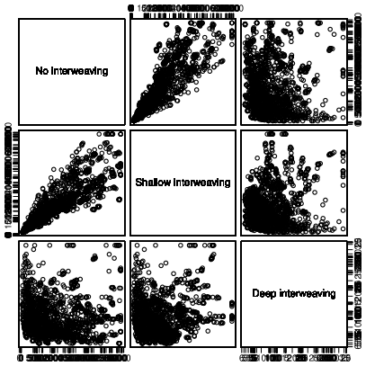
Figure 2: Left: Boxplots of estimated inefficiency factors for posterior draws from $p(\Lambda_{11}|\bm{y}^{[i]})$ where $\bm{y}^{[i]},i\in\{1,\dots,100\}$, denote artificially generated data sets whose underlying parameters are identical, cf. Table A.2.1 in Appendix A.2. Right: Pairwise scatter plots thereof.

Moreover, when investigating performance of MCMC samplers through simulation studies, it is of great importance to take sample variation into account; even when identical parameter values are used for the generation of latent variables and data, sampling (in)efficiency may vary greatly. To illustrate this, we show box plots of the inefficiency factors stemming from repeated data generating processes in the left panel of Figure 2. Note the enormous range for the standard sampler; depending on the data, IFs of $5000$ or more are not uncommon, while at the same time IFs of around $100$ can be observed. However, independently of the actual data, interweaving attenuates this effect drastically and increases efficiency uniformly. The right panel of Figure 2 shows pairwise scatter plots of these IFs. Note that shallow interweaving yields efficiency improvements which are more or less independent of the actual data (around five-fold for all data sets), whereas deep interweaving IFs appear less clearly correlated.

	1	2
1	2901.87
2	2630.89	999.88
3	2931.02	233.08
4	2936.83	673.08
5	2909.98	876.57
6	2772.16	934.87
7	2303.80	958.02
8	1463.70	968.13
9	605.16	974.56
10	113.16	976.10

(a) No interweaving

	1	2
1	462.07
2	434.09	186.39
3	460.59	80.57
4	457.71	141.30
5	451.84	164.85
6	437.95	174.34
7	406.73	178.91
8	337.78	181.54
9	215.53	183.30
10	67.89	184.30

(b) Shallow interweaving

	1	2
1	8.56
2	10.81	8.69
3	8.48	10.92
4	8.55	9.00
5	8.79	8.46
6	9.33	8.25
7	10.38	8.19
8	12.36	8.17
9	16.07	8.14
10	22.07	8.18

(c) Deep interweaving

Table 1: Average IFs for factor loadings matrix $\bm{\Lambda}$.

	$f_{1,1000}$	$f_{2,1000}$	$h_{11,1000}$	$h_{12,1000}$
No interweaving	121.54	53.30	232.23	21.59
Shallow interweaving	48.98	20.42	127.24	16.27
Deep interweaving	3.79	3.76	5.44	5.85

Table 2: Average IFs for the final factors $f_{jT}$ and their log-variances $h_{m+j,T}$, $j\in\{1,2\}$.

To provide a more complete picture, we list the inefficiency factors for all elements of $\bm{\Lambda}$ for the various algorithms in Table 1, averaged over all $100$ runs. Note that shallow interweaving permits efficiency gains of around two- to eight-fold as opposed to the standard sampler, whereas deep interweaving delivers gains up to around $400$-fold.

It comes as no surprise that sampling (in)efficiencies of draws for the volatility parameters $\mu_{i}$, $i\in\{1,\dots,m\}$ as well as $\phi_{i}$ and $\sigma_{i}$, $i\in\{1,\dots,m+r\}$ are not affected substantially by this interweaving strategy, thus they are not reported here. It is however worth noting that the inefficiency of factor ${\bm{f}}_{j,\bullet}$ and factor log-variance draws ${\bm{h}}_{m+j,\bullet}$, $j\in\{1,\dots,r\}$ may be influenced by bad mixing of $\bm{\Lambda}$. For illustration, IFs are reported for the final factors $f_{1T}$ and $f_{2T}$ and their log-variances $h_{m+1,T}$ and $h_{m+2,T}$ in Table 2.

Figure 3: Log predictive Bayes factors in favor of the $r$-factor model over the no-factor model. The first $500$ returns in the data set are treated as prior information and log one-day-ahead predictive likelihoods are accumulated over the following $500$ days. Circles connected with a solid line indicate values obtained with completely unrestricted loadings matrices; triangles connected with dashed lines indicate values where the loadings matrix is restricted to be lower triangular.

To conclude the simulation exercise, we investigate predictive performance of under- and overfitting models through cumulative log predictive Bayes factors in Figure 3; see Kastner (2017) for computational details. It stands out that the biggest predictive gain over a model that ignores contemporaneous correlations comes from introducing the first factor, i.e. allowing for co-volatility through one common factor. Then, as expected, the second factor bumps the predictive score to its maximum. After that, it remains (almost) constant for three and more factors, irrespectively of whether the lower triangular restriction is enforced or not. This points out that underfitting models are severly worse in terms of prediction while overfitting models hardly suffer from the extra parameters introduced.

Note that, similar to a scree plot in principal component analysis, Figure 3 can also be used as a graphical tool for finding the appropriate number of factors. For this exercise, we clearly find the true number of two factors.

5 Application to Exchange Rate Data

AUD	Australia dollar	CAD	Canada dollar	CHF	Switzerland franc
CNY	China yuan renminbi	CZK	Czech R. koruna	DKK	Denmark krone
GBP	UK pound	HKD	Hong Kong dollar	HRK	Croatia kuna
HUF	Hungary forint	IDR	Indonesia rupiah	JPY	Japan yen
KRW	South Korea won	MYR	Malaysia ringgit	NOK	Norway krone
NZD	New Zealand dollar	PHP	Philippines peso	PLN	Poland zloty
RON	Romania fourth leu	RUB	Russia ruble	SEK	Sweden krona
SGD	Singapore dollar	THB	Thailand baht	TRY	Turkey lira
USD	US dollar	ZAR	South Africa rand

Table 3: Currency abbreviations.

In this section, we analyze exchange rates with respect to EUR. Data was obtained from the European Central Bank’s Statistical Data Warehouse and ranges from April 1, 2005 to August 6, 2015. It contains $m=26$ (all which were available for this time frame) daily exchange rates on $2650$ days listed in Table 3. For further analysis, we thus use $T=2649$ demeaned log returns. The data is displayed in Figure A.3.1 in Appendix A.3. Common “stylized facts” of financial time series are clearly visible; note e.g. the obvious volatility clustering during 2008 and 2009 and again throughout late 2014 and early 2015. To put the robustness of our sampler to the test, we use the data as-is, i.e. without excluding series containing extreme outliers such as the CHF spike on January 14, 2015 or the near collapse of RUB around December 16, 2014.

5.1 Model Specification

For selecting the number of factors in this application, it is important to keep in mind the primary purpose of the analysis. Different sampling strategies are applied, depending on whether identification of $\bm{\Lambda}$ is of no concern (e.g. for covariance matrix prediction only), or whether identification is instrumental for understanding the unobserved, underlying factors.

For the first case, we experimented with fitting unrestricted models to the exchange rates data. This implies that the method is completely invariant to series ordering and there are no model-implied “leading factors” as is usually the case. With respect to selecting the number of factors, we found that higher-order models without any restriction on the factor loadings matrix yield higher marginal likelihoods and are thus recommended. Figure 4 illustrates this via log predictive Bayes factors.

Figure 4: Log predictive Bayes factors in favor of the $r$-factor model over the no-factor model. The first $1000$ returns in the data set are treated as prior information and log one-day-ahead predictive likelihoods are accumulated over the following $1000$ days. Circles connected with a solid line indicate values obtained with completely unrestricted loadings matrices; triangles connected with dashed lines indicate values where the loadings matrix is restricted to be lower triangular. The component series are ordered alphabetically.

If identification is warranted, an important step is the appropriate ordering of the variables, before the usual lower triangular structure is imposed on the factor loadings matrix to guarantee mathematical identifiability, as outlined in Section 2.2. This, however, makes inference on the factor loadings matrix dependent on the appropriate ordering of the variables. We exemplify this by the predictive Bayes factors for models where the component series are ordered alphabetically and the lower triangular structure is imposed on the first three series appearing in Table 3, namely AUD, CAD and CHF. As shown in Figure 4, for a given number of factors $r$, the log predictive Bayes factors of the constrained models are consistently smaller than for the unrestricted models, indicating that a purely mathematical identifiability constraint may be in conflict with the data.

Also for the constrained models, the log predictive Bayes factors are ever increasing for the exchange rate data. However, it stands out that the relative gain per additional factor is highest for few factors, flattening out quickly. Furthermore, draws of the factor loading matrix in these higher-order models are difficult to identify, in particular, if the lower triangular constraint is in conflict with the data and spurious factors, i.e. factors which are significantly loaded on by only few series, are present (see Frühwirth-Schnatter and Lopes, 2017, for a detailed discussion of this issue in the static factor context). Thus, to keep presentation feasible and to avoid spurious factors, we restrict ourselves to a model with $r=4$ factors for the following in-depth discussion.

One way to find constraints that are not in conflict with the data is to post-process the MCMC draws of an unrestricted sampler with $r=4$ factors, a method that has been applied in Conti et al. (2014) and Aßmann et al. (2016). Note that rather than reordering the variables before imposing a lower triangular constraint, we can choose three (out of the 26) currencies, and impose the $r(r-1)/2=6$ zero restrictions on the corresponding factor loadings, see e.g. Dunn (1973). While the choice of these currencies is not unique, inference is robust to specific choices, as long as the corresponding currencies serve as “leaders” for specific factors. This is exemplified by Figure A.3.3 which displays the posterior median of the MCMC draws of the factor loadings obtained from an unrestricted sampler with $r=4$. To solve column switching, the columns of $\bm{\Lambda}$ are rearranged by the size of their maximum median loading. According to Figure A.3.3 in Appendix A.3, USD is a definite candidate to lead factor one, PLN leads a second factor, and AUD leads a third factor. Alternatively, identification could be based on any other currency strongly loading on factor 1 (such as HKD or CNY), in combination with HUF (instead of PLN) and NZD (instead of AUD).

Prior hyperparameters are the same as for the simulation study in Section 4. A sensitivity analysis shows that none of the hyperparameter choices turn out to be very influential in this particular application with the exception of the prior factor loadings variances $B_{\Lambda}$. These, however, are only important for the absolute scaling of the factors and do not notably influence the relative loadings sizes or predictive Bayes factors. We run each sampler for $550\,000$ iterations, discard the first $50\,000$ draws as burn-in, leaving $500\,000$ which we use for posterior inference. Even after this substantial amount of iterations, it is not clear that the sampler without interweaving has properly converged; we therefore omit its presentation. IFs from the interwoven samplers are presented in Table A.3.1 in Appendix A.3.

Finally, we identify the signs of the loadings in the post-processing phase by investigating the MCMC draws. For each factor, the series whose posterior absolute loadings distribution is furthest away from zero is assigned a positive sign, the other loadings are aligned thereafter, see also Section A.1.4 in Appendix A.1.

5.2 Posterior Factor Volatilities and their Loadings

We begin by discussing the log-variances of the latent factors, visualized in Figure 6, alongside the corresponding factor loadings whose marginal posterior distributions are depicted in Figure 6 and whose posterior means are listed in Table 4.

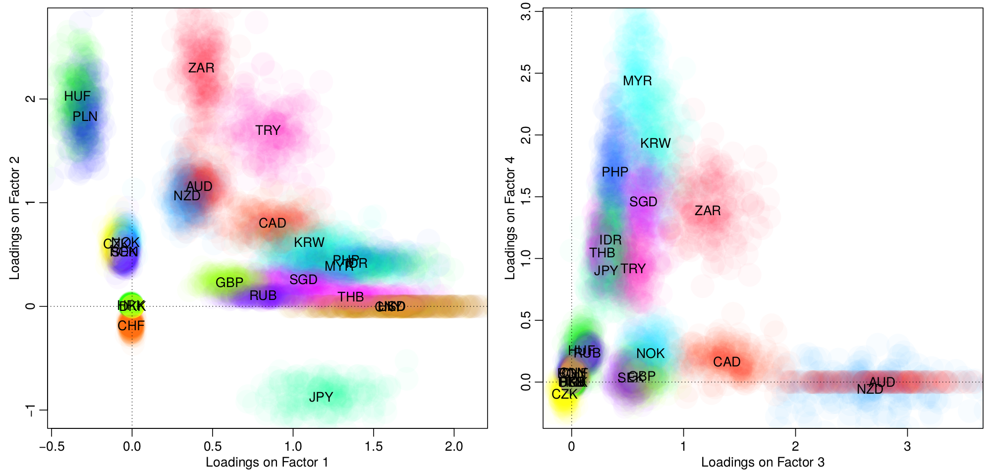
Figure 5: Marginal posteriors of the factor log-variances $h_{m+j,t},j=1,\dots,4$ ($\text{mean}\pm 2\times\text{sd}$).

Figure 6: Marginal posterior distribution of the factor loadings, visualized through arbitrarily colored scatterplots of MCMC draws.

$\bm{\Lambda}_{\bullet,1}$ $\bm{\Lambda}_{\bullet,2}$ $\bm{\Lambda}_{\bullet,3}$ $\bm{\Lambda}_{\bullet,4}$ AUD 0.418 1.156 2.772 * CAD 0.873 0.805 1.389 CHF -0.184 CNY 1.592 0.076 CZK -0.099 0.605 DKK 0.002 GBP 0.605 0.230 0.627 HKD 1.611 0.003 0.005 HRK HUF -0.339 2.028 IDR 1.395 0.419 0.347 1.153 JPY 1.176 -0.875 0.310 0.904 KRW 1.100 0.617 0.750 1.935

$\bm{\Lambda}_{\bullet,1}$ $\bm{\Lambda}_{\bullet,2}$ $\bm{\Lambda}_{\bullet,3}$ $\bm{\Lambda}_{\bullet,4}$ MYR 1.285 0.391 0.587 2.439 NOK 0.619 0.704 NZD 0.342 1.066 2.665 PHP 1.330 0.449 0.389 1.702 PLN -0.292 1.835 * * RON -0.051 0.530 RUB 0.813 0.104 0.138 0.237 SEK -0.049 0.529 0.527 SGD 1.065 0.260 0.642 1.463 THB 1.358 0.092 0.273 1.049 TRY 0.845 1.702 0.549 0.920 USD 1.614 * * * ZAR 0.431 2.303 1.219 1.390

Table 4: Posterior means of $p(\bm{\Lambda}|{\bm{y}})$, in alphabetical order. Blank entries signify that the respective marginal distribution is not bound away from zero with at least 99% posterior probability. Starred entries are those which have been set to zero a priori.

The first factor can clearly be interpreted as the USD-driven one, as the pegged triplet USD, CNY and HKD loads very highly on this factor, alongside many other currencies. Its volatility is generally very smooth, rising in the aftermath of the 2008 financial crisis and going down again after 2009; a second increase can be seen in the second half of 2014, possibly in connection with the Greek government-debt crisis. Factor 2’s log-variance appears slightly less persistent and more volatile, it is driven by ZAR, the only African currency in the sample, alongside Eastern Europe’s / Southwestern Asia’s HUF, PLN and TRY. Interestingly, JPY loads negatively on this factor. The third factor shows a similar overall pattern as the first. The highest loading series for this factor are AUD and NZD, emphasizing the Trans-Tasman relations. Other commodity currencies such as ZAR and CAD also load highly on this factor. Factor 4 is clearly driven by the currencies of the Tiger Cub economies such as MYR, KRW, PHP and SGD.

5.3 Posterior Volatilities and Correlations

In order not to overload the graphical displays used to visualize the results of the analysis, we display the results for a two-year period only for the rest of this section. More specifically, we look at the years 2008 and 2009, covering the most volatile span during the financial crisis. Irrespectively of that, the full data set has been used for estimation and other time spans could be displayed analogously.

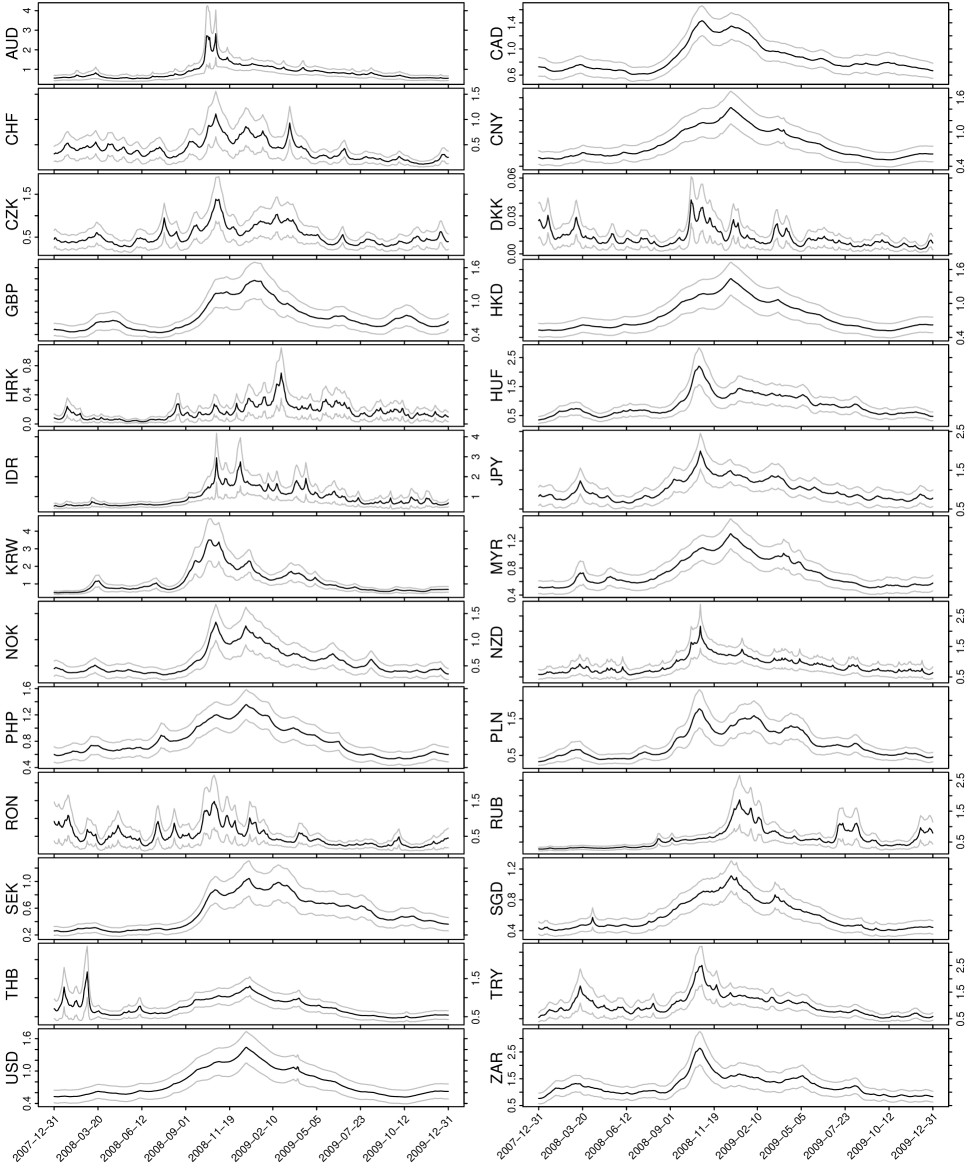
Figure 7: Posterior volatilities of exchange rate log returns with respect to EUR, from the last day of 2007 until the last day of 2009 ($\text{mean}\pm 2\times\text{sd}$).

We start out by visualizing the marginal posterior means of univariate volatilities for all $26$ currencies in Figure 7 from the last day of 2007 until the last day of 2009. Series such as DKK or HRK are (very) closely pegged to EUR and unsurprisingly show very low volatility throughout the crisis. Other European currencies (CHF, RON, SEK, CZK) follow suit. Tiger Cub economies such as PHP, HKD, THB, and MYR align very closely with USD and CNY. The most volatile currencies during this period are KRW, ZAR, IDR, JPY, and also TRY, followed by NZD, AUD, and CAD. Overall, it stands out that even though some series-specific ups and downs can be spotted, a common trend is clearly visible.

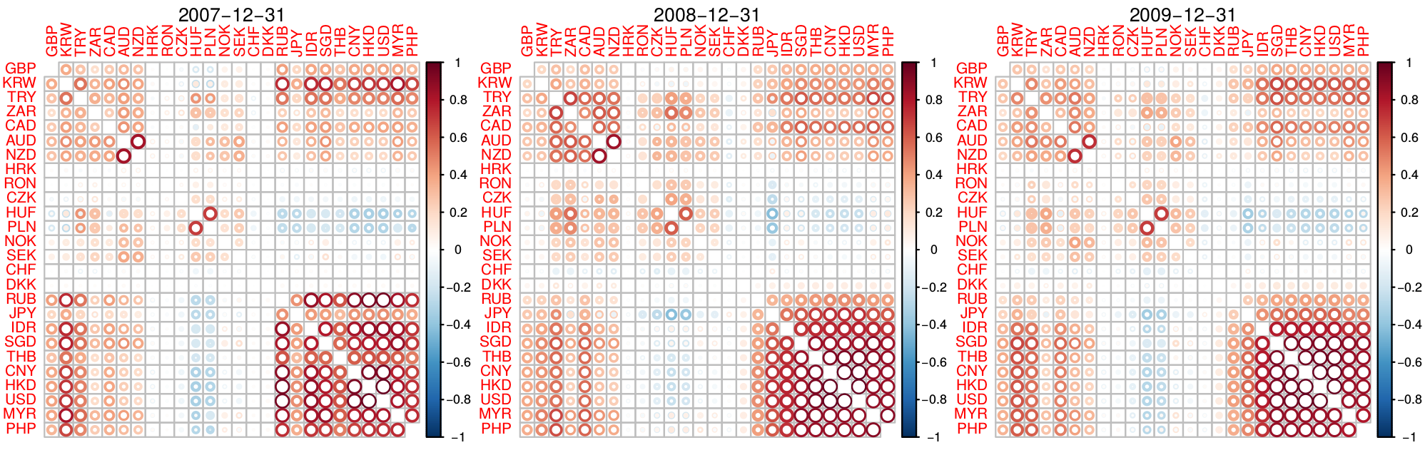
Figure 8: Posterior correlation matrices on the last trading days of 2006, 2007, and 2008. For each element, the size of the outer/inner circle is determined by the posterior mean plus/minus two posterior standard deviations, thereby indicating posterior uncertainty. Color and opacity are determined by the posterior mean. The remaining days are visualized in a video to be found online at https://vimeo.com/212887492.

Next, implied correlation matrices are displayed in Figure 8, exemplified for the last day of 2007, 2008, and 2009. Additionally to displaying the mean posterior pairwise correlations (at the given dates) via color and shading, these plots visualize posterior uncertainty; the outer and inner circles’ sizes correspond to $\text{posterior mean}\pm 2\text{ standard deviations}$, respectively. The images were generated using the R package corrplot (Wei, 2016); its option hclust (hierarchical clustering) was used for ordering the series to emphasize the blocks of currencies.

To further illustrate variability over time, we determine the posterior means of the pairwise time-varying correlations of USD against the other currencies which are plotted in Figure A.3.2 in Appendix A.3. As was to be expected, correlations of CNY and HKD with USD are almost always very close to one; IDR, THB, SGD, MYR, and PHP show rather high correlation throughout. The correlation between USD and RUB on the other hand falls from around $0.9$ in early 2008 to around $0.4$ in late 2009, whereas THB moves in the opposite direction; its correlation with USD is around $0.5$ at the beginning of the time window and increases quickly to around $0.9$. Eastern European non-euro currencies, in particular PLN and HUF, appear to be slightly negatively correlation with USD throughout the entire period.

6 Conclusion and Outlook

Estimating time-varying (dynamic) covariance and correlation matrices of financial and economic time series constitutes a current and active area of research. One of the main challenges thereby is the curse of dimensionality, i.e. the fact that the number of elements of these matrices grows quadratically with the number of observed series. We address this issue by imposing a low-dimensional latent factor structure where the factors are allowed to exhibit stochastic volatility and thereby govern co-movement of volatility over time. To conduct reliable statistical inference, we propose novel Bayesian MCMC algorithms which exploit the model-inherent identifiability constraints. By interweaving different (but mathematically equivalent) parameterizations, the proposed strategies substantially improve mixing of draws obtained from the posterior distribution, in particular for the factor loadings matrix. The method proposed is fully automatic in the sense that the end-user is not required to manually adjust any tuning parameters.

In an extensive case study discussing exchange rates with respect to EUR we show that the algorithm plays well with real-world data that exhibits a fair degree of outliers (e.g. CHF, RUB) which are captured through the idiosyncratic stochastic volatility components. The model structure allows for a covariance decomposition in four interpretable factors (USD/CNY driven, Eastern Europe, commodity currencies, Tiger Cub economies). These, alongside the idiosyncratic volatilities, drive the dynamics of the joint correlation structure. The pairwise correlations with USD range from “almost perfect” (CNY, HKD) over “hardly existent” (CHF, HRK) to “slightly negative” (PLN, HUF) with a varying and time-dependent degree of variability.

Concerning extensions of the model, we point out that due to the modular nature of MCMC, all the ideas of this paper can be straightforwardly generalized to models that independently model the mean, be it through a simple nonzero mean vector, a local level model, external regressors, or via (vector) autoregressive processes. For models where the level of the returns explicitly depends on the (co-)volatilities (volatility-in-mean-type-effects, see e.g. Chan, 2017) or the returns are assumed to be correlated with the (co-)volatilities (leverage-type-effects, see e.g. Ishihara and Omori, 2017), more involved estimation methods are required; this unfortunately places their discussion outside the scope of this paper. Nevertheless, due to the growing number of successful applications of interweaving methods in different contexts, there is good reason to hope for similar effects when they are used for these type of factor SV model extensions.

SUPPLEMENTARY MATERIAL

Web Appendix

containing (A.1) details of the various sampling steps of Algorithm 1 and details concerning the R package factorstochvol, (A.2) the data generating parameter values for the simulation study in Section 4, and (A.3) further results for the exchange rate data discussed in Section 5. (.pdf file)

Video

displaying the time-varying conditional correlation matrix distribution for the full data set (cf. Figure 8). Available at https://vimeo.com/212887492. (.avi file)

R-package

factorstochvol, version 0.8.3, containing code to run the samplers described in the paper. Available at https://cran.r-project.org/package=factorstochvol. (GNU zipped tar file)

Replication code

for the results in the paper, including the exchange rate data. (GNU zipped tar file)

Web Appendix to “Efficient Bayesian Inference
for Multivariate Factor Stochastic Volatility
Models”

Gregor Kastner

Department of Finance, Accounting and Statistics
WU Vienna University of Economics and Business, Austria
gregor.kastner@wu.ac.at

Sylvia Frühwirth-Schnatter
Department of Finance, Accounting and Statistics
WU Vienna University of Economics and Business, Austria
sfruehwi@wu.ac.at

Hedibert Freitas Lopes
Insper, Brazil
hedibertfl@insper.edu.br

Appendix A.1 Details on MCMC Sampling

A.1.1 Details on Updating the Volatilities

The latent equations

$$h_{it} = (1-\phi_{i})\mu_{i}+\phi_{i}h_{i,t-1}+\sigma_{i}\eta_{it},\qquad i=1,\ldots,m,$$ (A.1.1)

$$h_{m+j,t} = \phi_{m+j}h_{m+j,t-1}+\sigma_{m+j}\eta_{m+j,t},\qquad j=1,\ldots,r,$$ (A.1.2)

are combined with the (augmented) observation equation (3), yielding

$$\log(y_{it}-\bm{\Lambda}_{i,\bullet}{\bm{f}}_{t})^{2} = h_{it}+\log\varepsilon_{it}^{2},\qquad i=1,\ldots,m,$$ (A.1.3)

$$\log f_{jt}^{2} = h_{m+j,t}+\log\zeta_{jt}^{2},\qquad j=1,\ldots,r.$$ (A.1.4)

Due to the modular nature of MCMC methods, updating the latent log-variances ${\bm{h}}$ and the corresponding parameters appearing in (A.1.1) and (A.1.2) amounts to $m+r$ independent updates with augmented data appearing on the left hand side of (A.1.3) and (A.1.4).

Each of these $m+r$ models is a univariate stochastic volatility (SV) model as introduced by Taylor (1982). References about its efficient Bayesian estimation include Jacquier et al. (1994); Shephard (1994); Shephard and Pitt (1997); Kim et al. (1998); Omori et al. (2007); Strickland et al. (2008); McCausland et al. (2011); Kastner and Frühwirth-Schnatter (2014); Shestopaloff and Neal (2014). Consequently, the substantial amount of research on this matter which has emerged in the last two decades can directly be applied. In particular, we follow Kastner and Frühwirth-Schnatter (2014) and simply use the implementation in the R (R Core Team, 2017) package stochvol (Kastner, 2016c) as a “plug-in” for the factor SV sampler discussed in this paper (set dontupdatemu to TRUE for sampling factor volatilities). The SV update in stochvol can be accessed from R through the functions svsample and svsample2, whereas the latter is a stripped-down version of the former that omits input checking and post-processing. Moreover, in order to maximize execution speed when large models are to be fitted, C/C++ level access to the core update function is provided. Note that the number of function calls may be in the range of billions and more, thus even tiny costs for code interpretation can quickly accumulate. The R level interface was employed for prototyping and proof-of-concept implementations (cf. Kastner et al., 2014). For the results reported in this paper, direct access to update was used. A detailed description of this procedure is given in Kastner (2016a) and the package manual.

A.1.2 Details on Sampling the Loadings

Because $y_{it}\sim\mathcal{N}\!\left(\bm{\Lambda}_{i,\bullet}{\bm{f}}_{t},e^{h_{it}}\right)$, sampling the loadings conditionally on ${\bm{f}}$ constitutes a Bayesian regression problem with heteroscedastic errors. Letting $\tilde{r}_{i}$ denote the number of unrestricted elements in row $i$, rewriting yields

$$\tilde{\bm{y}}_{i}\sim\mathcal{N}_{T}\!\left(\bm{X}_{i}\bm{\Lambda}_{i,\bullet}^{\prime},{{\bm{I}}}_{T}\right),$$

where $\tilde{\bm{y}}_{i}=(y_{i1}e^{-h_{i1}/2},\dots,y_{iT}e^{-h_{iT}/2})^{\prime}$ denotes the $i$th normalized observation vector and

$$\bm{X}_{i}=\begin{bmatrix}f_{11}e^{-h_{i1}/2}&\cdots&f_{\tilde{r}1}e^{-h_{i1}/2}\\ \vdots&&\vdots\\ f_{1T}e^{-h_{iT}/2}&\cdots&f_{\tilde{r}T}e^{-h_{iT}/2}\end{bmatrix}$$

is the $T\times\tilde{r}_{i}$ design matrix. Thus, independently for each $i$, sampling from $\bm{\Lambda}_{i,\bullet}|{\bm{f}},{\bm{y}}_{i,\bullet},{\bm{h}}_{i,\bullet}$ is achieved by performing a Gibbs-update from

$$\bm{\Lambda}_{i,\bullet}^{\prime}|{\bm{f}},{\bm{y}}_{i,\bullet},{\bm{h}}_{i,\bullet},\sim\mathcal{N}_{\tilde{r}}\!\left(\bm{b}_{iT},\bm{B}_{iT}\right),$$

with $\bm{B}_{iT}=(\bm{X}_{i}^{\prime}\bm{X}_{i}+B_{\Lambda}^{-1}{{\bm{I}}}_{\tilde{r}_{i}})^{-1}$ and $\bm{b}_{iT}=\bm{B}_{iT}\bm{X}_{i}^{\prime}\tilde{\bm{y}}_{i}$.

A.1.3 Details on Sampling the Factors

Sampling the factors ${\bm{f}}_{t}$ for each $t=1,\ldots,T$ conditionally on the factor loadings $\bm{\Lambda}$ and the volatilities ${\bm{h}}_{t}$, i.e. from ${\bm{f}}_{t}|\bm{\Lambda},{\bm{y}}_{t},{\bm{h}}_{t}$, is again a standard Bayesian regression problem. We have

$$\tilde{\bm{y}}_{t}\sim\mathcal{N}_{m}\!\left(\bm{X}_{t}{\bm{f}}_{t},{{\bm{I}}}_{m}\right),$$

where $\tilde{\bm{y}}_{t}=(y_{1t}e^{-h_{1t}/2},\dots,y_{mt}e^{-h_{mt}/2})^{\prime}$ denotes the normalized observation vector at time $t$ and

$$\bm{X}_{t}=\begin{bmatrix}\Lambda_{11}e^{-h_{1t}/2}&\cdots&\Lambda_{1r}e^{-h_{1t}/2}\\ \vdots&&\vdots\\ \Lambda_{m1}e^{-h_{mt}/2}&\cdots&\Lambda_{mr}e^{-h_{mt}/2}\\ \end{bmatrix},$$

is the $m\times r$ design matrix. Independently for each $t$, the posterior is consequently given by

$${\bm{f}}_{t}|\bm{\Lambda},{\bm{y}}_{t},{\bm{h}}_{t}\sim\mathcal{N}_{r}\!\left(\bm{b}_{mt},\bm{B}_{mt}\right),$$

where $\bm{B}_{mt}=(\bm{X}_{t}^{\prime}\bm{X}_{t}+{\bm{V}}_{t}({\bm{h}}^{V}_{t})^{-1})^{-1}$ and $\bm{b}_{mt}=\bm{B}_{mt}(\bm{X}_{t}^{\prime}\tilde{\bm{y}}_{t})$.

A.1.4 Sign Identification

For sensible interpretation of the factor loadings their signs have to be identified. If done a posteriori, this requires the selection of one series per factor whose loadings distribution is sufficiently bound away from zero. For the paper at hand, we simply investigate the absolute values of the posterior draws from the loadings distribution. For each factor, the series whose smallest absolute MCMC draw is largest gets assigned a positive sign which in turn implies the signs for all other loadings on this factor. In other words, letting $K$ denote the number of MCMC draws after burn-in, in order to identify factor $j=1,\dots,r$, we assign a positive sign to the posterior distribution of $|\Lambda_{ij}|$, where $i$ is chosen to be

$$\operatorname*{arg\,max}_{i\in\{1,\ldots,m\}}\left(\min_{k\in\{1,\ldots,K\}}\left|\Lambda_{ij}^{(k)}\right|\right).$$

Subsequently, we align the other loadings on factor $j$ accordingly. To achieve this behavior in factorstochvol, use signident with method = "maximin". In order to simply use the leading factors to identify the loadings, use signident with method = "diagonal". For the exchange rate data, the sign of factor 1 is identified via USD, factor 2 via ZAR, factor 3 via AUD, and factor 4 via MYR.

A.1.5 A Note on Implementation

High-dimensional models, in particular models with many latent variables, pose a non-negligible computational challenge to those aiming for efficient MCMC implementations. In principle, each individual MCMC step can be straightforwardly computed in parallel. In practice, however, doing so is only useful in shared memory environments (e.g. through multithreading/multiprocessing) as the increased communication overhead in distributed memory environments easily outweighs the speed gains. Apart from within-steps-parallelization, MCMC is of intrinsically iterative nature in the sense that posterior draws are generated conditionally on older draws. Thus, they cannot be parallelized straightforwardly and call for compiled and optimized programming languages to avoid the cost of code interpretation at every iteration. Moreover, memory access needs to be optimized, as large amounts of latent variable draws must be stored either temporary (if required only for the next conditional draws) or more permanently (if required for direct posterior inference). In this paper, we tackle the computational burden by using high-performance C and C++ code, interfaced to R via RcppArmadillo (Eddelbuettel and Sanderson, 2014). Additionally to providing an interface between R and C++, RcppArmadillo also accommodates fast linear algebra routines by means of the Armadillo library (Sanderson, 2010). For ease-of-use, all code is bundled in the R package factorstochvol (Kastner, 2016b) which is available on the Comprehensive R Archive Network (CRAN).

Appendix A.2 Simulation Study

The data generating parameter values for the simulation study in Section 4 are listed in Table A.2.1.

$\bm{\Lambda}_{\text{true}}$	1	2
1	1.00
2	0.90	1.00
3	0.80	0.10
4	0.70	0.20
5	0.60	0.30
6	0.50	0.40
7	0.40	0.50
8	0.30	0.60
9	0.20	0.70
10	0.10	0.80

(a) Factor loadings

	$\mu_{\text{true}}$	$\phi_{\text{true}}$	$\sigma_{\text{true}}$
1	-2.00	0.80	0.60
2	-1.90	0.82	0.55
3	-1.80	0.84	0.50
4	-1.70	0.86	0.45
5	-1.60	0.88	0.40
6	-1.50	0.90	0.35
7	-1.40	0.92	0.30
8	-1.30	0.94	0.25
9	-1.20	0.96	0.20
10	-1.10	0.98	0.15

(b) Idiosyncratic volatility parameters

	$\phi_{\text{true}}$	$\sigma_{\text{true}}$
1	0.99	0.10
2	0.95	0.30

(c) Factor volatility parameters

Table A.2.1: Data generating values.

Appendix A.3 Application to Exchange Rate Data

This section provides additional results for exchange rate data analyzed in Section 5. Figure A.3.1 depicts the raw data. The pairwise correlations of USD against the other currencies as implied by the model discussed in detail in the main paper are plotted in Figure A.3.2. Inefficiency factors for posterior draws from the factor loadings using the interwoven samplers, i.e. deep and shallow interweaving, are presented in Table A.3.1. Finally, Figure A.3.3 visualizes the posterior medians of the factor loadings in a $4$-factor model without any restrictions on the factor loadings matrix. The factor ordering has been determined through a post-processing procedure; factors are sorted according to their average median posterior loadings.

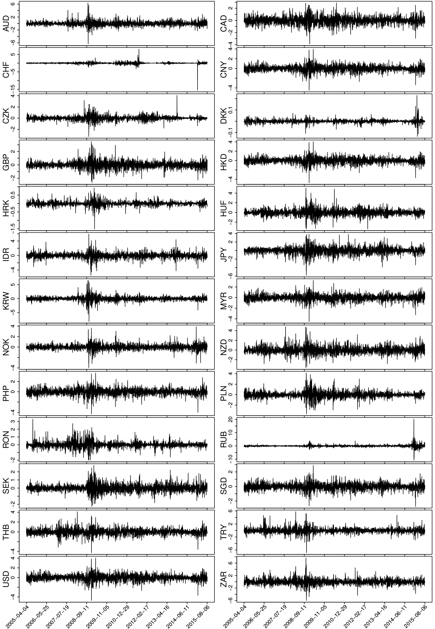
Figure A.3.1: Demeaned log returns of EUR exchange rates.

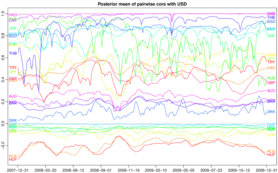
Figure A.3.2: Posterior means of pairwise correlations with USD.

	$\bm{\Lambda}_{\bullet,1}$	$\bm{\Lambda}_{\bullet,2}$	$\bm{\Lambda}_{\bullet,3}$	$\bm{\Lambda}_{\bullet,4}$
AUD	414	588	901	*
CAD	704	608	842	25
CHF	8	203	38	25
CNY	784	12	21	128
CZK	207	770	28	19
DKK	99	7	23	6
GBP	719	176	717	9
HKD	786	40	74	72
HRK	11	10	13	5
HUF	399	861	58	30
IDR	770	525	386	609
JPY	749	661	129	228
KRW	752	555	669	812
MYR	766	420	582	911
NOK	28	618	665	28
NZD	315	526	881	56
PHP	784	557	417	813
PLN	388	903	*	*
RON	70	710	26	14
RUB	780	224	189	146
SEK	39	630	600	11
SGD	785	356	803	898
THB	780	82	483	753
TRY	694	824	342	230
USD	786	*	*	*
ZAR	358	855	608	340

(a) Shallow interweaving

	$\bm{\Lambda}_{\bullet,1}$	$\bm{\Lambda}_{\bullet,2}$	$\bm{\Lambda}_{\bullet,3}$	$\bm{\Lambda}_{\bullet,4}$
AUD	32	49	29	*
CAD	26	40	27	17
CHF	6	45	28	14
CNY	27	9	11	27
CZK	18	47	10	9
DKK	10	7	10	5
GBP	25	24	24	9
HKD	27	36	35	34
HRK	5	6	6	5
HUF	27	47	50	16
IDR	26	39	23	30
JPY	26	39	40	24
KRW	26	38	26	31
MYR	26	43	28	34
NOK	16	38	24	13
NZD	34	46	28	51
PHP	26	39	23	32
PLN	26	49	*	*
RON	16	42	26	10
RUB	26	28	18	22
SEK	15	39	24	12
SGD	27	42	29	33
THB	26	25	25	32
TRY	26	42	29	23
USD	27	*	*	*
ZAR	27	43	26	24

(b) Deep interweaving

Table A.3.1: Estimated inefficiency factors for posterior draws of the factor loadings.

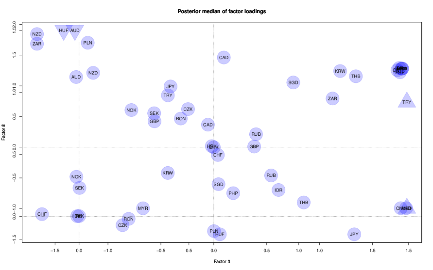
Figure A.3.3: Posterior medians of the factor loadings in the unrestricted model. The factors have been ordered according to their average posterior median loadings. An up-pointing triangle means that this series was used for sign-identification in the horizontal direction, a down-pointing triangle means it was used for sign-identification in the vertical direction.

References

- Aguilar and West (2000) Aguilar, O. and M. West (2000). Bayesian dynamic factor models and portfolio allocation. Journal of Business & Economic Statistics 18(3), 338–357.
- Aßmann et al. (2016) Aßmann, C., J. Boysen-Hogrefe, and M. Pape (2016). Bayesian analysis of static and dynamic factor models: An ex-post approach toward the rotation problem. Journal of Econometrics 192(1), 190–206.
- Bitto and Frühwirth-Schnatter (2016) Bitto, A. and S. Frühwirth-Schnatter (2016). Achieving shrinkage in a time-varying parameter model framework. arxiv pre-print 1611.01310v1.
- Chan (2017) Chan, J. (2017). The stochastic volatility in mean model with time-varying parameters: An application to inflation modeling. Journal of Business & Economic Statistics 35(1), 17–28.
- Chib et al. (2006) Chib, S., F. Nardari, and N. Shephard (2006). Analysis of high dimensional multivariate stochastic volatility models. Journal of Econometrics 134(2), 341–371.
- Conti et al. (2014) Conti, G., S. Frühwirth-Schnatter, J. J. Heckman, and R. Piatek (2014). Bayesian exploratory factor analysis. Journal of Econometrics 183(1), 31–57.
- Dunn (1973) Dunn, J. E. (1973). A note on sufficiency condition for uniqueness of a restricted factor matrix. Psychometrika 38(1), 141–143.
- Eddelbuettel and Sanderson (2014) Eddelbuettel, D. and C. Sanderson (2014). RcppArmadillo: Accelerating R with high-performance C++ linear algebra. Computational Statistics and Data Analysis 71, 1054–1063.
- Frühwirth-Schnatter and Lopes (2017) Frühwirth-Schnatter, S. and H. F. Lopes (2017). Parsimonious Bayesian factor analysis when the number of factors is unknown. Technical report.
- Frühwirth-Schnatter and Wagner (2010) Frühwirth-Schnatter, S. and H. Wagner (2010). Stochastic model specification search for Gaussian and partial non-Gaussian state space models. Journal of Econometrics 154(1), 85–100.
- Geweke and Zhou (1996) Geweke, J. and G. Zhou (1996). Measuring the pricing error of the arbitrage pricing theory. The Review of Financial Studies 9(2), 557–587.
- Ghosh and Dunson (2009) Ghosh, J. and D. B. Dunson (2009). Default prior distributions and efficient posterior computation in Bayesian factor analysis. Journal of Computational and Graphical Statistics 18(2), 306–320.
- Han (2006) Han, Y. (2006). Asset allocation with a high dimensional latent factor stochastic volatility model. Review of Financial Studies 19(1), 237–271.
- Harvey et al. (1994) Harvey, A. C., E. Ruiz, and N. Shephard (1994). Multivariate stochastic variance models. Review of Economic Studies 61(2), 247–264.
- Hörmann and Leydold (2013) Hörmann, W. and J. Leydold (2013). Generating generalized inverse Gaussian random variates. Statistics and Computing 24(4), 1–11.
- Ishihara and Omori (2017) Ishihara, T. and Y. Omori (2017). Portfolio optimization using dynamic factor and stochastic volatility: Evidence on fat-tailed error and leverage. The Japanese Economic Review 68(1), 63–94.
- Jacquier et al. (1994) Jacquier, E., N. G. Polson, and P. E. Rossi (1994). Bayesian analysis of stochastic volatility models. Journal of Business & Economic Statistics 12(4), 371–389.
- Jungbacker and Koopman (2006) Jungbacker, B. and S. J. Koopman (2006). Monte Carlo likelihood estimation for three multivariate stochastic volatility models. Econometric Reviews 25(2–3), 385–408.
- Kastner (2016a) Kastner, G. (2016a). Dealing with stochastic volatility in time series using the R package stochvol. Journal of Statistical Software 69(5), 1–30.
- Kastner (2016b) Kastner, G. (2016b). factorstochvol: Bayesian estimation of (sparse) latent factor stochastic volatility models. R package version 0.8.3.
- Kastner (2016c) Kastner, G. (2016c). stochvol: Efficient Bayesian inference for stochastic volatility (SV) models. R package version 1.3.2.
- Kastner (2017) Kastner, G. (2017). Sparse Bayesian time-varying covariance estimation in many dimensions. arxiv pre-print 1608.08468.
- Kastner and Frühwirth-Schnatter (2014) Kastner, G. and S. Frühwirth-Schnatter (2014). Ancillarity-sufficiency interweaving strategy (ASIS) for boosting MCMC estimation of stochastic volatility models. Computational Statistics and Data Analysis 76, 408–423.
- Kastner et al. (2014) Kastner, G., S. Frühwirth-Schnatter, and H. F. Lopes (2014). Analysis of exchange rates via multivariate Bayesian factor stochastic volatility models. In E. Lanzarone and F. Ieva (Eds.), The Contribution of Young Researchers to Bayesian Statistics – Proceedings of BAYSM2013, Volume 63 of Springer Proceedings in Mathematics & Statistics, pp. 181–186. Springer.
- Kim et al. (1998) Kim, S., N. Shephard, and S. Chib (1998). Stochastic volatility: Likelihood inference and comparison with ARCH models. Review of Economic Studies 65(3), 361–393.
- Leydold and Hörmann (2015) Leydold, J. and W. Hörmann (2015). GIGrvg: Random variate generator for the GIG distribution. R package version 0.4.
- Liesenfeld and Richard (2006) Liesenfeld, R. and J.-F. Richard (2006). Classical and Bayesian analysis of univariate and multivariate stochastic volatility models. Econometric Reviews 25(2–3), 335–360.
- Lintner (1965) Lintner, J. (1965). The valuation of risk assets and the selection of risky investments in stock portfolios and capital budgets. The Review of Economics and Statistics 47(1), 13–37.
- Lopes and Carvalho (2007) Lopes, H. F. and C. M. Carvalho (2007). Factor stochastic volatility with time varying loadings and Markov switching regimes. Journal of Statistical Planning and Inference 137(10), 3082–3091.
- Lopes and West (2004) Lopes, H. F. and M. West (2004). Bayesian model assessment in factor analysis. Statistica Sinica 14(1), 41–67.
- McCausland et al. (2011) McCausland, W. J., S. Miller, and D. Pelletier (2011). Simulation smoothing for state-space models: A computational efficiency analysis. Computational Statistics and Data Analysis 55(1), 199–212.
- Nakajima and West (2013) Nakajima, J. and M. West (2013). Dynamic factor volatility modeling: A Bayesian latent threshold approach. Journal of Financial Econometrics 11(1), 116–153.
- Nardari and Scruggs (2007) Nardari, F. and J. T. Scruggs (2007). Bayesian analysis of linear factor models with latent factors, multivariate stochastic volatility, and APT pricing restrictions. Journal of Financial and Quantitative Analysis 42(4), 857–891.
- Omori et al. (2007) Omori, Y., S. Chib, N. Shephard, and J. Nakajima (2007). Stochastic volatility with leverage: Fast and efficient likelihood inference. Journal of Econometrics 140(2), 425–449.
- Papaspiliopoulos et al. (2007) Papaspiliopoulos, O., G. Roberts, and M. Sköld (2007). A general framework for the parameterization of hierarchical models. Statistical Science 22(1), 59–73.
- Pitt and Shephard (1999) Pitt, M. K. and N. Shephard (1999). Time-varying covariances: A factor stochastic volatility approach. In J. M. Bernardo, J. O. Berger, A. P. Dawid, and A. F. M. Smith (Eds.), Bayesian Statistics 6 – Proceedings of the Sixth Valencia International Meeting, pp. 547–570. Oxford: Oxford University Press.
- Plummer et al. (2006) Plummer, M., N. Best, K. Cowles, and K. Vines (2006). CODA: Convergence diagnosis and output analysis for MCMC. R News 6(1), 7–11.
- R Core Team (2017) R Core Team (2017). R: A Language and Environment for Statistical Computing. R Foundation for Statistical Computing.
- Ross (1976) Ross, S. A. (1976). The arbitrage theory of capital asset pricing. Journal of Economic Theory 13(3), 341–360.
- Sanderson (2010) Sanderson, C. (2010). Armadillo: An open source C++ linear algebra library for fast prototyping and computationally intensive experiments. Technical Report, NICTA.
- Sentana and Fiorentini (2001) Sentana, E. and G. Fiorentini (2001). Identification, estimation and testing of conditionally heteroskedastic factor models. Journal of Econometrics 102(2), 143–164.
- Sharpe (1964) Sharpe, W. F. (1964). Capital asset prices: A theory of market equilibrium under conditions of risk. The Journal of Finance 19(3), 425–442.
- Shephard (1994) Shephard, N. (1994). Partial non-Gaussian state space. Biometrika 81(1), 115–131.
- Shephard (1996) Shephard, N. (1996). Statistical aspects of ARCH and stochastic volatility. In D. R. Cox, O. E. Barndorff-Nielsen, and D. V. Hinkley (Eds.), Time Series Models in Econometrics, Finance and Other Fields, pp. 1–67. London: Chapman & Hall.
- Shephard and Pitt (1997) Shephard, N. and M. K. Pitt (1997). Likelihood analysis of non-Gaussian measurement time series. Biometrika 84(3), 653–667.
- Shestopaloff and Neal (2014) Shestopaloff, A. Y. and R. M. Neal (2014). Efficient Bayesian inference for stochastic volatility models with ensemble MCMC methods. Technical report.
- Simpson (2015) Simpson, M. (2015). Application of interweaving in DLMs to an exchange and specialization experiment. In S. Frühwirth-Schnatter, A. Bitto, G. Kastner, and A. Posekany (Eds.), Bayesian Statistics from Methods to Models and Applications – Research from BAYSM 2014, Volume 126 of Springer Proceedings in Mathematics & Statistics, pp. 75–90. Springer.
- Simpson et al. (2017) Simpson, M., J. Niemi, and V. Roy (2017). Interweaving Markov chain Monte Carlo strategies for efficient estimation of dynamic linear models. Journal of Computational and Graphical Statistics 26(1), 152–159.
- Strickland et al. (2008) Strickland, C. M., G. M. Martin, and C. S. Forbes (2008). Parameterisation and efficient MCMC estimation of non-Gaussian state space models. Computational Statistics and Data Analysis 52(6), 2911–2930.
- Taylor (1982) Taylor, S. J. (1982). Financial returns modelled by the product of two stochastic processes: A study of daily sugar prices 1691–79. In O. D. Anderson (Ed.), Time Series Analysis: Theory and Practice 1, pp. 203–226. Amsterdam: North-Holland.
- van Dyk and Meng (2001) van Dyk, D. and X.-L. Meng (2001). The art of data augmentation. Journal of Computational and Graphical Statistics 10(1), 1–50.
- Wei (2016) Wei, T. (2016). corrplot: Visualization of a correlation matrix. R package version 0.77.
- Yu and Meng (2011) Yu, Y. and X.-L. Meng (2011). To center or not to center: that is not the question—an ancillarity-suffiency interweaving strategy (ASIS) for boosting MCMC efficiency. Journal of Computational and Graphical Statistics 20(3), 531–570.
- Zhou et al. (2014) Zhou, X., J. Nakajima, and M. West (2014). Bayesian forecasting and portfolio decisions using dynamic dependent sparse factor models. International Journal of Forecasting 30(4), 963–980.