Holographic Curvature Perturbations in a Cosmology with a Space-Like Singularity

Abstract

We study the evolution of cosmological perturbations in an anti-de-Sitter (AdS) bulk through a cosmological singularity by mapping the dynamics onto the boundary conformal fields theory by means of the AdS/CFT correspondence. We consider a deformed AdS space-time obtained by considering a time-dependent dilaton which induces a curvature singularity in the bulk at a time which we call $t=0$, and which asymptotically approaches AdS both for large positive and negative times. The boundary field theory becomes free when the bulk curvature goes to infinity. Hence, the evolution of the fluctuations is under better controle on the boundary than in the bulk. To avoid unbounded particle production across the bounce it is necessary to smooth out the curvature singularity at very high curvatures. We show how the bulk cosmological perturbations can be mapped onto boundary gauge field fluctuations. We evolve the latter and compare the spectrum of fluctuations on the infrared scales relevant for cosmological observations before and after the bounce point. We find that the index of the power spectrum of fluctuations is the same before and after the bounce.

I Introduction

In spite of its many successes, cosmology faces a number of outstanding theoretical and fundamental challenges. One of the most fundamental questions that remain to be answered in cosmology is the singularity problem. Singularities appear in many cosmological models and are unavoidable in some contexts like Einstein gravity with matter fields that do not violate the null energy condition (NEC). Both Standard Big Bang cosmology and the inflationary universe scenario Guth realized in the context of scalar field matter coupled to classical General Relativity are examples where an initial Big Bang singularity is present (see the classic paper Hawking for the proof that an initial singularity appears in Standard Big Bang cosmology and Borde for an extension to inflationary cosmology). Bouncing cosmologies, alternative scenarios for the evolution of the universe where a contraction period precedes the expansion of the universe, also have singularities at the bounce point, at least if they are realized within the realm of Einstein or dilaton gravity coupled to matter obeying the NEC. One can avoid Big Bang/Big Crunch singularities by postulating matter which violates the NEC (see e.g. quintom ; ghost ; Galileon for some specific models, and RHBmbRev for a review), or by going beyond, Einstein gravity (e.g. by choosing gravitational Lagrangians with specifically chosen higher derivative terms BM , by considering the Horava-Lifshitz gravitational action HLbounce , or by assuming certain nonlocal gravitational Lagrangians Biswas ). However, there are doubts as to whether these constructions can be embedded in a consistent quantum theory of gravity Adams . A consistent understanding of singularity resolution can presumably only be studied in such an ultraviolet complete theory, superstring theory being the prime example.

In this context the AdS/CFT correspondence could come to use. This correspondence Maldacena is a proposal for a non-perturbative treatment of string theory and states that the dynamics of a bulk Anti-de Sitter (AdS) space-time that includes gravity is encoded in the boundary of this space-time, where a conformal field theory (CFT) with no gravity lives. This conjecture has been used in many different fields of physics, from black hole physics to condensed matter, with great success (for a review e.g. AdS-CFTrev ). It has already been proposed in the literature that the AdS/CFT correspondence could be used to resolve cosmological singularities HH ; CHT ; CHTproblem ; CHT2 , specially in the context of singular bouncing models such as the Pre-Big-Bang PBB and Ekpyrotic Ekp scenarios.

Bouncing cosmologies have recently been studied extensively as possible alternatives to cosmological inflation for producing the fluctuations which we are currently mapping out with observations. If the equation of state of matter in the contracting phase has $w>-1/3$, where $w$ is the ratio of pressure to energy density, then scales exit the Hubble radius during contraction. Hence, it is possible to have a causal generation mechanism for fluctuations in the same way as in inflationary cosmology, where scales exit the Hubble radius in an expanding phase if the equation of state of matter obeys $w<-1/3$. As was pointed out in FB ; Wands , if the equation of state of matter during the time interval when scales which are measured now in cosmological observations exit the Hubble radius has the equation of state $w=0$ (i.e. a matter-dominated equation of state), then initial vacuum perturbations originating on sub-Hubble scales acquire a scale-invariant spectrum, the kind of spectrum which fits observations well . A scale-invariant spectrum of fluctuations can also be obtained in the Pre-Big-Bang PBBsi and in the Ekpyrotic NewEkp scenarios, making use of entropy modes. The major problem in these analyses is that the fluctuations have to be matched from the contracting phase to the expanding phase across a singularity (for singular bouncing cosmologies) or in the region of high curvature (in nonsingular models in which new physics provides a nonsingular bounce) where the physics is not under controle. This is the second place where the AdS/CFT correspondence could become useful: the boundary theory becomes weakly coupled precisely where the bulk theory becomes strongly coupled, and hence we can expect that the evolution of the fluctuations on the boundary will be better behaved.

We here consider a time-dependent deformation of AdS DT1 ; DT2 ; DT3 ; DT4 (see also CH1 ; CH2 ) which yields a contracting phase with increasing curvature leading to a bulk singularity at a time which we call $t=0$. The evolution for $t>0$ is the mirror inverse of what happens for $t<0$. This means that the bulk is expanding with decreasing curvature. The challenge for our work hence is to explore if the AdS/CFT correspondence can be used to determine the cosmological perturbations in the expanding phase starting with some initial cosmological perturbations in the contracting phase. In the case of a singular bouncing bulk cosmology this question cannot be answered from the point of view of the bulk evolution of those perturbations, and in a non-singular bouncing setup the evolution in the bulk cannot be reliably computed in a perturbative approach. For example, there are ambiguities if one wants to apply the matching condition approach HV ; DM to connect early time to late time fluctuations (see e.g. DV ). The goal of our work is to avoid these difficulties in the bulk evolution in the strongly coupled region by mapping the dynamics onto the boundary theory which is weakly coupled near $t=0$. The AdS/CFT correspondence presents an unique opportunity to understand the effects of a bulk singularity on cosmological observables. Specifically, we are interested in computing the amplitude and slope of the spectrum of cosmological perturbations after the bounce given the spectrum before the bounce.

In Brandenberger:2016egn the authors studied the evolution of matter scalar field perturbations using the AdS/CFT correspondence in a deformed AdS₅ spacetime, where a spacelike singularity is present. This background spacetime is a time dependent background studied before in DT1 ; DT2 ; DT3 ; DT4 where the dilaton bulk field has a time dependence which as $t\rightarrow 0$ produces a curvature singularity. The bulk theory is weakly coupled for $|t|>t_{b}$ and strongly coupled for smaller values of $|t|$. In the context of this background the authors studied dilaton perturbations on a hypersurface perpendicular to the AdS radial coordinate, starting with a scale invariant spectrum on super-Hubble scales at early times $t<-t_{b}$. When bulk gravity becomes strongly coupled at $t=-t_{b}$, the perturbations were mapped to the boundary theory, a $\mathcal{N}=4$ Super Yang-Mills (SYM) theory, and the fluctuations of the corresponding boundary fields were then evolved from $t=-t_{b}$ to $t=t_{b}$. This SYM model has a time-dependent coupling constant that goes to zero at the same time as the singularity occurs in the bulk. However, in spite of the fact that the boundary theory becomes free at $t=0$, it was found that infinite particle production occurs between $t=-t_{b}$ and $t=0$. Thus, it was necessary to introduce a cutoff: the coupling constant was kept finite but small in a short period of time $|t|<\xi$ around the singularity, where $\xi\ll t_{b}$. This made it possible to evolve the fluctuations unambiguously past the time $t=0$ where the bulk singularity occurs until the late time $t=t_{b}$ after the singularity after which the bulk theory becomes weakly coupled again. After that, for the infrared modes that are of cosmological interest (and whose wavelength is much larger than the Hubble radius already at the time $t=-t_{b}$), the bulk scalar field perturbations were reconstructed. It was found that the late time scalar field perturbations have a scale invariant spectrum, showing that the spectral index does not change while passing through the region of the highly curved (and maybe even singular) bulk. On the other hand, the amplitude of the scalar field perturbation spectrum is amplified - a consequence of the squeezing of the perturbation modes on super-Hubble scales in the contracting phase.

The evolution of scalar matter perturbations is interesting since it offers us a good guide as to the evolution of gravitational waves . However, of more interest in cosmology is the spectrum of the scalar metric perturbations, since those lead to the adiabatic density perturbations responsible for structure formation in the universe. The goal of the present paper is to extend the analysis of Brandenberger:2016egn to the case of cosmological perturbations.

Scalar cosmological perturbations are more complicated to analyze than matter scalar field fluctuations. They are made up of a combination of metric and matter inhomogeneities which take different forms in different coordinate systems. In the case of purely adiabatic perturbations the information about the inhomogeneities is most conveniently encoded in the quantity $\mathcal{R}$, the curvature perturbation in comoving gauge (the gauge in which the matter field fluctuation vanishes Bardeen ), a quantity that remains constant in time outside the Hubble radius BST ; BK ; Lyth ; AB ; LV .

According to the AdS/CFT dictionary, the metric perturbation $\delta g_{\mu\nu}$ has as its dual operator in the CFT the expectation value of the boundary energy momentum tensor. In order to reconstruct the curvature perturbations (which are a combination of the metric and the matter fluctuations) in the future of the space-time singularity, one needs to know the full evolution of the boundary operators corresponding to both the bulk matter scalar field and the metric perturbations.

We argue in this paper that there exists a gauge choice that can simplify this problem. We generalize the spatially flat gauge to the $5$-dimensional case. This gauge allows us to describe the curvature perturbations as a function only of the perturbations of the scalar field, that represents the matter in our space-time. We do this by using the gauge freedom to gauge away the metric perturbations degrees of freedom which leaves us with only the scalar field perturbations. Because of this choice of gauge we only need to know how the scalar field perturbations behave at late times. This allows us to perform the same analysis as in Brandenberger:2016egn , and to evolve the perturbations of a scalar field using the boundary theory in a singular deformed AdS₅ space-time. With this gauge choice, the analysis of scalar field fluctuations is all we need to be able to reconstruct the curvature perturbations in the future of the space-time singularity.

This paper is organized as follows. Section II contains a summary of the dynamics of the deformed AdS bulk space-time containing a spacelike singularity. In Section III we discuss the cosmological perturbations in this deformed AdS₅ space-time and present the generalized spatially flat gauge. Section IV shows the main result, namely how to obtain the curvature perturbation at late times evolving from an initial bulk perturbation using the AdS/CFT correspondence. We find that the spectral index is not changed when comparing the spectrum at late and early times, but that there is an increase in amplitude resulting from the squeezing of the Fourier mode wave functions.

II Bulk Dynamics

We are interested in studying cosmological backgrounds in the context of the AdS/CFT correspondence. Some time-dependent backgrounds in string theory were studied in DT1 ; DT2 ; DT3 ; DT4 where the bulk solution can be thought as a time-dependent deformation of $AdS_{5}\times S^{5}$ with a corresponding $\mathcal{N}=4$ supersymetric Yang-Mills (SYM) theory with a time dependent gauge coupling constant as a dual theory.

This background bulk solution can be described by the line element

$$ds^{2} = \frac{\ell^{2}}{z^{2}}\left(dz^{2}+\tilde{g}_{ab}dx^{a}dx^{b}\right)$$ (1)

$$= \frac{\ell^{2}}{z^{2}}\left[dz^{2}+\frac{2|\tau|}{3\ell}\left(-d\tau^{2}+\delta_{ij}dx^{i}dx^{j}\right)\right]\,,\quad\quad t\gtrless 0,\;z\in(0,+\infty)\,,$$

plus a $d\Omega^{2}_{5}$ term representing the $S^{5}$ factor. In the second line we are choosing a special Kasner type solution. Note that $\tau$ denotes conformal time.The dilaton profile is given by

$$\phi(x)=\phi(t)=\sqrt{3}\ln\left(\frac{|t|}{\ell}\right)\,,\quad\Rightarrow\quad e^{\phi(x)}=\left(\frac{|t|}{\ell}\right)^{\sqrt{3}}\,,$$ (2)

with $\ell$ being the AdS scale. Throughout this paper we use conventions that Greek letters $\mu,\nu,\dots$ run over all of the five space-time indices $0,\dots 4$ with $z$ the AdS radial dimension; latin indices from the beginning of the alphabet $a,b,\dots$ run over the indices $0,\dots,3$ corresponding to the four-dimensional space-time perpendicular to the AdS radial direction, and Latin letters $i,j,\dots$ run over the spatial indices $1,2,3$.

This solution can be embedded in a solution of a $10$-dimensional type IIB supergravity theory provided that the metric and the dilaton satisfy the equations of motion

$$\partial_{\mu}\left(\sqrt{-\tilde{g}}\tilde{g}^{\mu\nu}\partial_{\nu}\phi(x)\right)=0,\quad R_{ab}[\tilde{g}]=\frac{1}{2}\nabla_{a}\Phi\nabla_{b}\phi(x)\,.$$ (3)

The bosonic sector of this embedding includes a RR $5$-form flux which supports the $S^{5}$ tensor factor of the space-time. The $S^{5}$ factor will not play a role in the following and we will thus not track it further.

The element (1) is easily recognized to be a deformation of the line element of pure AdS in Poicaré coordinates, where the AdS coordinate runs from $z=0$ at the boundary to $z=\infty$ at the Poincaré horizon. In pure AdS the induced metric on constant-$z$ hypersurfaces is the Minkowski metric. In our solution the induced metric is instead composed of two copies of a Friedmann-Robertson-Walker (FRW) metric, as seen in (1), one for $t<0$ describing a collapsing geometry, and another for $t>0$ describing an expanding geometry. The solution contains a spacelike singularity, ”Big Crunch” singularity, at $t=0$. It is also singular as $z\to\infty$ at any fixed $t\neq 0$. This can be seen in Figure  1. Due to this latter fact, the spacetime cannot be Cauchy-extended beyond the Poincaré horizons which bound the coordinate chart. The string coupling is given by $g_{s}=e^{\phi(x)}$ and goes to zero at the singularity. If the singularity can be resolved by mapping the dynamics to the boundary, we will have a stringy realization of a boucing scenario.

We are assuming the the bulk universe initially begins in an AdS vacuum at some early moment $t_{i}$ and the background is given by a weakly coupled supergravity theory. At the moment $-t_{b}$, the bulk gravity becomes strongly coupled but at the same time the boundary gauge theory become weakly coupled. Hence, after the time $-t_{b}$ the evolution on the boundary becomes tractable in perturbation theory. On the future side of the bulk singularity, the boundary theory remains tractable perturbatively until the time $t_{b}$ when the the bulk theory becomes weakly coupled again at the cost of the boundary theory becoming strongly coupled. At that time we can reconstruct the bulk information (at least in the vicinity of the boundary) from boundary data (see e.g. Hamilton1 ; Hamilton2 ; Kabat ; Ian ).

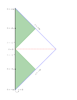
Figure 1: Conformal diagram of the background space-time. The spacelike singularities is shown in red. The vertical axis is time $t$, the horizontal direction represents the coordinate $z$ (with the boundary on the left side). If there were no deformation of $AdS$, the region drawn would correspond to the Poincare patch of $AdS$. The green regions may be covered by Fefferman-Graham FG charts with Minkowski boundary metrics.

We will take our space-time to be the hypersurface of some constant AdS radial coordinate $z$. We will be interested in considering linear fluctuations of matter and scalar metric degrees of freedom on this surface at some initial time $t\ll-t_{b}$, and computing the corresponding fluctuations on the same constant $z$ surface in the future of the singularity, once the bulk theory once again becomes weakly coupled, i.e. at $t=t_{b}$.

To resolve the singularity in the background (1, 2) and study the evolution of perturbations to the future of $t=-t_{b}$ we will map the problem onto the boundary using the AdS/CFT dictionary. We can see that the boundary of this $5$ dimensional solution is conformally flat and has a second order pole as $z\rightarrow 0$. So, in order to do holography we must specify a conformal frame, i.e. we must provide a defining function $\Omega(x)$ which behaves like $O(z^{2})$ as $z\to 0$, and which in turn selects the induced boundary metric $h_{ab}(x)$ via

$$ds^{2}_{bndry}:=h_{ab}(x)dx^{a}dx^{b}=\lim_{z\to 0}\Omega^{2}(x)\gamma_{ab}(x)dx^{a}dx^{b}\,,$$ (4)

where $\gamma_{ij}$ is the metric of a maximally symmetric three-dimensional hypersurface (the metric of Euclidean three space, of the three sphere or the three-dimensional hypersphere). The above is an asymptotic solution in Fefferman-Graham form FG that represents the conformal structure. There are two natural choices for $\Omega(x)$. First, if we select

$$\Omega_{\rm FRW}(x)=\frac{z}{\ell},$$ (5)

then the boundary limit is particularly simple and the conformal boundary has metric $h_{ab}(x)=\gamma_{ab}(x)$. We refer to this as the FRW frame. A second choice is

$$\Omega_{\rm M}(x)=\left(\frac{3z^{2}}{2\ell|t|}\right)^{1/2}\,.$$ (6)

With this choice the boundary metric is flat. We refer to this as the Minkowski frame. It is important to realize that $\Omega_{M}(x)$ is singular as $t\to 0$, and as a result the conformal transformation implied by $\Omega_{M}(x)$ is singular. One of our basic assumptions is that this conformal transformation is nevertheless a symmetry of the CFT.

Let us now turn to the CFT description of our solution. In this time-dependent background, the dual boundary theory is a $\mathcal{N}=4$ SYM theory with a source. Following the usual dictionary Skenderis:2000in , the AdS-Neumann part of $\phi(x)$ sets the value of the Yang-Mills coupling via

$$g^{2}_{YM}(x)=\lim_{z\to 0}e^{\phi(x)}\,.$$ (7)

In the Minkowski frame, this theory lives in flat space. Note that when the non-normalizable part of $\phi(x)$ varies with time, as in our example, the SYM theory in the boundary is sourced by a coupling that is time-dependent. So, the time dependent dilaton in the bulk corresponds to a time-dependent Yang-Mills coupling in the boundary. This coupling goes to zero as $t\rightarrow 0$ and the CFT becomes free.

III Cosmological Perturbations in the Deformed AdS₅

We want to compute the cosmological perturbations from the space-time described above. In Brandenberger:2016egn , we perturbed only the scalar field, namely, the dilaton, and treated the perturbations of the dilaton. However, to fully describe the cosmological perturbations, we need to include the perturbations of the metric. For this, we need to perturb this deformed AdS₅ metric (see e.g. 5dflucts for general discussions of cosmological fluctuations in brane world like five dimensional space-times).

Our starting point is the perturbed five-dimensional space-time metric

$$g_{MN}\,=\,g_{MN}^{(0)}\,+\,\delta g_{MN}\,,$$ (8)

where the first term on the right hand side denotes the background metric which depends only on $t$ and $z$, and the second the linear fluctuations (which depend on all five space-time coordinates).

We can make a field redefinition in order to write the background metric in the following way:

$$ds^{2}\,=\,d\bar{z}^{2}+\tilde{g}_{ab}d\bar{x}^{a}d\bar{x}^{b}\,,$$ (9)

where $\bar{z}=(l/z)z$ and $\bar{x}^{\mu}=(l/z)x^{\mu}$. In some papers in the literature this is called a Gaussian normal coordinate system, and it is equivalent to restrict the coefficient in front of the $z$-part of the metric to be unity. In the following we will drop the tilde signs on the coordinates.

After including linear fluctuations, the metric can be written, performing the usual scalar-vector-tensor decomposition with respect to spatial rotations on the constant $z$ spatial hypersurface, as (see e.g. MFB ; RHBfluctrev )

$$ds^{2}\,=\,-dz^{2}(1+C_{0})+C_{a}dx^{a}+a^{2}(\tau)\left[\left(1+2\Phi\right)d\bar{\tau}^{2}-2B_{i}d\bar{x}^{i}d\bar{\tau}-\left(\delta_{ij}+h_{ij}\right)\right]dx^{i}dx^{j}\,,$$ (10)

where $\tau$ is the conformal time given by $d\tau=dt/a(t)$, and $\Phi,B_{i}$ and $h_{ij}$ are functions of all space-time variables. The linear quantities $C_{0}$ and $C_{a}$ are new metric fluctuations associated with the presence of the radial AdS direction. We can further decompose the $3-$vector $B_{i}$ into a scalar and a divergenceless part and the rank-$2$ symmetric tensor $h_{ij}$ into scalar, a vector and tensor parts:

$$B_{i}\, = \,\partial_{i}B+\hat{B}_{i}$$ (11)

$$h_{ij}\, = \,2\Psi\delta_{ij}+2\left(\partial_{i}\partial_{j}-\frac{1}{3}\delta_{ij}\nabla^{2}\right)E+\left(\partial_{i}\hat{E}_{j}+\partial_{j}\hat{E}_{i}\right)+2\hat{E}_{ij}\,,$$

where this decomposition is irreducible since the hatted quantities are divergenceless, $\partial^{i}\hat{E}_{i}$ and $\partial^{i}\hat{E}_{ij}=0$, and the tensor part is traceless, $\hat{E}^{i}_{i}=0$. Note that the tensor $\hat{E}_{ij}$ corresponds to gravitational waves, $\hat{B}_{i}$ and $\hat{E}_{j}$ to vector perturbations, and the remaining functions $\Phi,\Psi,B$ and $E$ to the scalar metric perturbations. This perturbed metric and the variables are analogous to the fluctuations in a usual $4$-dimensional cosmology when restricted to constant $z$ slices. However, one needs to remember that the quantities calculated also depend of the coordinate $z$. In the following we will neglect vector perturbations and gravitational waves.

Together with the metric perturbations, we need to perturb the energy-momentum tensor of the $5$-dimensional bulk. The matter content in our case is the dilaton field. This can be perturbed as follows, as in Brandenberger:2016egn

$$\bar{\phi}\left(z,\mathbf{x},t\right)\,=\,\phi\left(z,\mathbf{x},t\right)+\delta\phi\left(z,\mathbf{x},t\right)\,,$$ (12)

where $\phi$ represents the background dilaton field and $\delta\phi$ its linear perturbation.

General relativity allows for a freedom in the choice of the coordinate system. At the linearized level the space of coordinate transformation is five-dimensional, allowing us to impose five gauge conditions in order to remove residual gauge degrees of freedom. As is done in the four space-time dimensional theory of cosmological perturbations we use two of these gauge freedoms to simplify the scalar sector of the metric. One choice is longitudinal gauge in which one sets $B=E=0$. Two gauge degrees of freedom are vector from the point of view of the constant $z$ hypersurfaces and can be used to reduce the number of vector modes, and the remaining gauge degree of freedom involves the $z$ direction and could be used to set $C_{0}=0$. Making these choices, the scalar cosmological fluctuations involve the variables $\Phi,\Psi$ and $\delta\phi$ (plus the variables $C_{a}$ which will not be important for us). An alternative choice is to pick the spatially flat gauge (uniform curvature gauge) in which the curvature on the constant time (and $z$) hypersurfaces is constant in space. In the absence of anisotropic stress $\Phi$ and $\Psi$ coincide, and the Einstein constraint equation related the other two variables . Hence, on a fixed $t$ and $z$ hypersurface, the information about scalar cosmological perturbations is encoded in terms of a single function.

Our goal will be to compute the evolution of the $3+1$ dimensional curvature fluctuation variable $\mathcal{R}$, which in the absence of entropy fluctuations is conserved on super-Hubble scales and thus encodes the relevant information about the scalar cosmological perturbations. It is hence the useful variable to track on super-Hubble scales, the scales we are interested in in this work (and also the ones which are of interest in inflationary cosmology).

We choose to work in uniform curvature gauge. In this gauge, the variable $\mathcal{R}$ is on super-Hubble scales given by

$$\mathcal{R}\,=\,-\frac{\mathcal{H}}{\phi^{\prime}}\delta\phi\,.$$ (13)

in terms of the scalar field fluctuation $\delta\phi$. The coefficient relating $\mathcal{R}$ and $\delta\phi$ is given by the comoving Hubble constant and by the background scalar field. Note that a prime indicated the derivative with respect to conformal time.

The variance for $\mathcal{R}$ in this gauge is given by the variance of $\delta\phi$. For each Fourier mode we have

$$\langle|\mathcal{R}_{k}|^{2}\rangle\,=\,\left(\frac{\mathcal{H}}{\phi^{\prime}}\right)^{2}\langle|\delta\phi_{k}|^{2}\rangle\,.$$ (14)

IV Holographic Curvature Perturbation at Late Times

The goal of the section is to calculate the conserved curvature perturbation in our deformed spacetime at late times. With the general spatially flat gauge developed above, we are able to write the curvature perturbation in terms of the perturbations of the scalar field and its background value. This is important in our setup, since it avoids one having to understand how the metric perturbations evolve holographically in this singular spacetime.

In our previous work Brandenberger:2016egn , we showed a prescription for obtaining the bulk perturbation of a scalar field $\delta\phi$, the dilaton in our case, at late times $t>t_{b}$ in the weakly coupled region of the expanding period, given initial conditions for the perturbations of the scalar field in the bulk in the weakly coupled contracting phase. We were interested to understand how the presence of the singularity affects the initial scalar field perturbations. In particular, we investigated if the power spectrum given in the bulk at past times is changed after the singularity. We showed that the final spectrum of $\delta\phi_{k}$ remains scale invariant, given it was scale invariant in the past.

We now show how to use the results of our previous work to compute the quantity that is of interest in cosmology, the curvature perturbation. As we saw in the previous section, then when working in the uniform spatial curvature gauge we only need the power spectrum of the scalar field to obtain the power spectrum $P_{\mathcal{R}}$ of the curvature perturbations

$$P_{\mathcal{R}}\,=\,\left(\frac{\mathcal{H}}{\phi^{\prime}}\right)^{2}P_{\delta\phi}=\frac{1}{2\pi^{2}}k^{3}\left(\frac{\mathcal{H}}{\phi^{\prime}}\right)^{2}|\delta\phi_{k}\left(z,t\right)|^{2}\,.$$ (15)

Thus, if we have the solution of the bulk scalar field in the future of the singularity, $\delta\phi_{k}(+t_{b})$, we are able to obtain the power spectrum of the curvature perturbation from the above relation.

As it was shown in Brandenberger:2016egn , the bulk scalar field fluctuations in the future of the singulariy can be locally reconstructed from the boundary data via Hamilton1 ; Hamilton2

$$\delta\phi\left(t,x,z\right)\,=\,\int dt^{\prime}d^{3}yK\left(t^{\prime},y|t,x,z\right)\mathcal{O}\left(t^{\prime},y\right)\,,$$ (16)

where the kernel $K\left(t^{\prime},y|t,x,z\right)$ is the smearing function. The important property of this smearing function is that its support is confined to the “AdS causal wedge”, i.e. to points with $|\delta t|\equiv t^{\prime}-t<z$ (see Fig. 2). The exact form of the smearing function will not be important for our analysis.This construction is similar to a boundary value problem (see also Ian ; Alberto ). This means that $\delta\phi\left(t,x,z\right)$ corresponds to a local operator $\mathcal{O}\left(y,t^{\prime}\right)$ in the CFT, with a map defined by the smearing function.

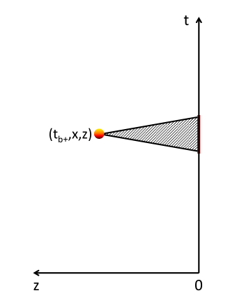
Figure 2: Sketch of the reconstruction process for bulk operators in the future of the singularity. The vertical axis is time, the horizontal axis indicates the radial coordinate $z$. The solid line is the boundary.The bulk field at a point with coordinates $(t_{b}^{+},x,z)$ is given by integrating the boundary data against the boundary-to-bulk propagator. The integration involves data in the shaded region only. The solid curves connecting the bulk point to the boundary are null geodesics.

We can make a translation in the time and space coordinates: $t^{\prime}=t+s$ and $y=x+y^{\prime}$. The smearing function is invariant under translations of the $x$ coordinates. In pure AdS it would also be invariant under time translations. In the case of our deformed AdS, the kernel has an explicit time-dependence. The important point is that the kernel has support within the AdS causal wedge. Hence, as long as we consider values of $z$ not too far from the boundary, the region of support of the kernel for the time $t=t_{b}$ is far away from the space-time singularity, and the kernel is hence well defined. The fact that the kernel is independent of the three dimensional spatial coordinates $x$ on the fixed $z$ surface implies that the kernel does not effect the shape of the power spectrum.

Our interest is to be able to find the spectrum of the perturbations in the future. For that, we need to work with the Fourier transform of (16). This is given by:

$$\delta\phi_{k}\left(z,t\right)\, = \int dsd^{3}y^{\prime}e^{-iky^{\prime}}K\left(t+s,y^{\prime}|z,t\right)\mathcal{O}\left(k,t+s\right)\,,$$ (17)

$$\simeq \int ds\underbrace{\int d^{3}y^{\prime}K\left(s+t,y^{\prime}|z,t\right)}_{M(t,s,z)}\mathcal{O}\left(k,t+s\right)$$

where in the last line we considered only the IR limit, the one of interest for cosmological perturbations. We can see from this equation that $\mathcal{O}\left(k,t+s\right)$ has the same $k$-dependence of $\delta\phi_{k}$, with the amplitude smeared and calculated at a translated time.

We do not need to know the exact form of the kernel for our deformed AdS₅. All we need to assume is the existence of such a smoothing function with a causal structure similar to the one for pure AdS (obtained in Hamilton1 ; Hamilton2 ). The differences would appear in the time-mode solution, since here we have FRW spacetime on the boundary instead of Minkowski, leading to a different normalization for $K(s,y^{\prime}|z)$. Also, this function has support on the causal wedge of $AdS$, and selects only data on the boundary that is space-like separated with $\mathbf{ky^{\prime}}<<1$, given by the values of $\mathbf{y^{\prime}}$ where the smearing function does not vanish. It is very important in our case that the only data necessary for the reconstruction of the bulk field is local, since the presence of the singularity makes part of the data in the past inaccessible in the future of the deformed AdS Poincare chart. We can see that from the green regions of Figure 1.

We can then write the power spectrum of the uniform curvature perturbation with respect to the boundary data. From equation (15), and knowing that for our bulk $\mathcal{H}=a^{\prime}/a$, where

$$a(\tau)\,=\,\frac{2}{3}\frac{|\tau|}{l}\,,$$ (18)

we have

$$P_{\mathcal{R}}(k,t) =\frac{1}{\left(2\pi l\right)^{2}}k^{3}|\delta\phi_{k}\left(z,t\right)|^{2}$$

$$=\frac{1}{\left(2\pi l\right)^{2}}k^{3}\left|\int dsM(s,z)\mathcal{O}\left(k,t+s\right)\right|^{2}\,.$$ (19)

Thus, the power spectrum of ${\mathcal{R}}$ has the same slope as that of the boundary operator ${\mathcal{O}}$. This boundary operator given in this equation is known from the AdS/CFT correspondence: The scalar field in the bulk corresponds to the expectation value of the trace of the square of the field strength of a conformal field theory living on the boundary:

$${\mathcal{O}}\,=\,\langle\mathrm{tr}F^{2}\rangle\,.$$ (20)

This is the same operator whose evolution was studied in our previous paper Brandenberger:2016egn , and in the following we will just briefly summarize the analysis which relates the late time spectrum of ${\mathcal{O}}$ with the initial spectrum of $\delta\phi$.

In our case, the boundary conformal field theory is a $\mathcal{N}=4$ Super Yang Mills (SYM) theory in $3+1$-dimensions with a Yang-Mills coupling that varies in time, inherited from the time-dependent dilaton from the bulk. Given this theory, we can evaluate the operator, since

$$F_{\mu\nu}\,=\,2\partial_{[\mu}A_{\nu]}-i\left[A_{\mu},A_{\nu}\right]\,.$$ (21)

We ignore the term with the commutator since this is subdominant in our analysis. We adopt Coulomb gauge ($\partial_{i}A^{i}=0$) and set $A_{0}=0$. Then the Fourier transform of the field strength tensor reduces to

$$\mathrm{Tr}[F^{2}(k,t)]\,=\,2\dot{A}_{k}^{2}-2(k_{j}A_{k_{i}})^{2}+2k_{i}A_{k_{j}}k^{j}A^{k_{i}}\,,$$ (22)

where summation over the index $k$ is implied. We are only interested in the infrared (IR) modes, where $k$ is small, so we can drop the last two term of the previous expression and thus obtain the approximate relation

$$\mathrm{Tr}[F^{2}(k,t)]\,=\,2\dot{A}_{k}^{2}\,.$$ (23)

where once again summation over $k$ is implied.

The fundamental field of this theory is the vector field $A_{\mu}$, and this can be evolved in time, given its equation of motion in the boundary. So, the field $A_{\mu}(+t_{b})$, necessary to calculate the operator $\mathcal{O}\left(x,t_{b}\right)$ can be evolved from a initial vector field through $t=0$, the time when the singularity happens. This time also corresponds to the place where the YM coupling vanishes and the theory becomes free.

Since the gauge theory becomes free, it could have been expected that the gauge field fluctuations pass through $t=0$ without any problem. However, as discussed in Brandenberger:2016egn this is not the case. In terms of the original Fourier space modes $A(k,t)$ there is a branch cut in the evolution equations, and in terms of the canonically normalized field corresponding to $A(k,t)$ there is in fact a divergence. This divergence corresponds to the blowup of particle production which is expected from the point of view of the bulk theory, where the fluctuation modes obtain infinite squeezing at $t=0$. Hence, it is not surprising that at the level of fluctuations the boundary theory at this point also becomes sick and infinite particle production occurs. This does not allow us to evolve the field passed $t=0$. In order to be able perform this evolution, we imposed a regularization of the YM coupling, making it constant during a period $\left[-\xi,\xi\right]$, where $\xi$ is smaller than $t_{b}$, and matching the solutions (and their first derivatives) in the periods $t<-\xi$, $-\xi<t<\xi$ and $t>\xi$.

We perform this matching in the boundary theory since in the bulk, at times $\xi=\sqrt{\alpha^{\prime}}$, where $\alpha^{\prime}$ is the string scale, the Ricci scalar reaches the string scale and the bulk supergravity description breaks down. So, matching in the boundary can be performed at time $\xi$, much closer to the singularity, where the bulk theory is already in the strong limit. Since the theory in the boundary has no gravity, this matching is under much better control and goes closer to the singularity than what could be done by working in the bulk.

With that, we can relate the solution of the field $A_{\mu}$ from early to late times past the singularity, first re-scaling the gauge field by $\tilde{A}_{k}(t)=e^{\phi/2}A_{k}(t)$ to obtain a canonically normalized field. The analysis of Brandenberger:2016egn yielded the result

$$\tilde{A}_{k}(t)=|t|^{\frac{1}{2}}\left[D_{J}^{+}J_{\nu_{g}}\left(|kt|\right)+D_{Y}^{+}Y_{\nu_{g}}\left(|kt|\right)\right]\,,$$ (24)

where the mode coefficients $D_{J}^{+}$ and $D_{Y}^{+}$ are related to the ones $D_{J}^{-}$ and $D_{Y}^{-}$before the singularity by:

$$D_{J}^{+} =\frac{1}{2\nu_{g}}D_{Y}^{-}+2^{-2\nu_{g}}\left(1+\frac{1}{2\nu_{g}}\right)\left(k\xi\right)^{2\nu_{g}}D_{J}^{-}\,,$$ (25)

$$D_{Y}^{+} =-\frac{1}{2\nu_{g}}D_{J}^{-}+2^{2\nu_{g}}\left(1-\frac{1}{2\nu_{g}}\right)\left(k\xi\right)^{-2\nu_{g}}D_{Y}^{-}\,.$$ (26)

At late times, at time $t=t_{b}$, when we map the results from the boundary to the bulk, the gauge field is then given by:

$$\tilde{A}_{k}(t_{b})\simeq\left(\frac{t_{b}}{\xi}\right)^{2\nu_{g}}\tilde{A}\left(-t_{b}\right)\,,$$ (27)

which means that the $k$-dependence if the field remains the same after passing through the singularity, changing only its amplitude that is enhanced by the factor

$$\mathcal{F}(t)\,=\,\left(t_{b}/\xi\right)^{2\nu_{g}}\,.$$ (28)

So, given an initial condition in the gauge field $A_{k}(-t_{b})$, we can time evolve this field until time $t_{b}$ in the future of the singularity, and then calculate the operator $\mathrm{Tr}\left[F^{2}(k,t^{\prime})\right]$ and obtain the power spectrum.

This initial value for the gauge field in the boundary theory can be inferred from the initial scalar field in the bulk. As done in our previous work, we choose a particular scaling of the Fourier modes of the boundary gauge field such that the operator $\mathcal{O}$ has the same amplitude and scaling as what is induced from the bulk scalar field fluctuations which we are starting out with. From (20) and (23) we have

$$m_{pl}^{4}\delta\phi^{in}(k)\,=\,\frac{1}{2}\int_{0}^{k}d^{3}k^{\prime}\dot{A}^{in}\left(\frac{k+k^{\prime}}{2}\right)\dot{A}^{in}\left(\frac{k-k^{\prime}}{2}\right)V^{1/2}\,=\,\mathrm{Tr}\left[F^{2}(-t_{b})\right]_{k}\,=\,\mathcal{O}\left(k,-t_{b}\right)\,,$$ (29)

where $V$ is a normalization volume introduced in the definition of the Fourier transform (such that the Fourier modes of $A$ have the mass dimension of a harmonic oscillator, i.e. $-1/2$). This integral can be performed in two regions, $R_{1}$ where $k<k^{\prime}$, and $R_{2}$ where $k>k^{\prime}$. In region $R_{1}$ we can set $k^{\prime}=0$ and get, approximately

$$m_{pl}^{4}\delta\phi^{in}(k)\,\sim\,k^{3}\dot{A}_{k}^{2}V^{1/2}\,.$$ (30)

In the case when the initial bulk scalar field has a scale invariant power spectrum, $\delta\phi\propto k^{-3/2}$, the gauge field at $t=-t_{b}$, the time of matching onto the boundary in the past, has $A_{k}^{in}(t)=A_{k}(-t_{b})\sim k^{-9/4}$. Assuming this scaling for the gauge Fourier modes, it can easily be seen that Region $R_{2}$ gives gives a contribution comparable to (30). With the initial conditions given by (29) and the growth of the gauge modes given by (27) we can write the boundary data in the future, encoded in the operator:

$$\mathcal{O}\left(k,t\right)\,=\,\frac{(4\nu_{g})^{2}}{\xi^{4\nu_{g}}}t^{2(2\nu_{g})}\frac{1}{2}\int_{0}^{k}d^{3}k^{\prime}\dot{A}\left(\frac{k+k^{\prime}}{2},-t_{b}\right)\dot{A}\left(\frac{k-k^{\prime}}{2},-t_{b}\right)V^{1/2}=\mathrm{Tr}\left[F^{2}(-t_{b})\right]_{k}\,.$$ (31)

Now we have all the ingredients to obtain the power spectrum of curvature perturbations past the singularity, given an initial bulk scalar field perturbation in the past:

$$P_{\mathcal{R}} =\frac{k^{3}}{\left(2\pi\right)^{2}}\left|\int dsM(s,z)\mathrm{Tr}\left[F^{2}(t_{b})\right]_{k}\right|^{2}\,,$$

$$=\frac{\left(4\nu_{g}\right)^{4}}{\left(2\pi\right)^{2}\xi^{8\nu_{g}}}\,k^{3}\,t^{4(2\nu_{g})}\left|\int dsM(s,z)\frac{1}{2}\int_{0}^{k}d^{3}k^{\prime}\dot{A}\left(\frac{k+k^{\prime}}{2},-t_{b}\right)\dot{A}\left(\frac{k-k^{\prime}}{2},-t_{b}\right)V^{1/2}\right|^{2}\,.$$ (32)

Integrating over region $R_{1}$, and taking $k^{\prime}=0$, we have

$$P_{\mathcal{R}} =\frac{\left(4\nu_{g}\right)^{4}}{\left(2\pi\right)^{2}\xi^{8\nu_{g}}}\,k^{3}\,t^{4(2\nu_{g})}\left|\int dsM(s,z)\,k^{3}\dot{A}^{2}(k,-t_{b})\right|^{2}\,,$$

$$=\frac{\left(4\nu_{g}\right)^{4}}{\left(2\pi\right)^{2}\xi^{8\nu_{g}}}\,k^{3}\,t^{4(2\nu_{g})}\left|\int dsM(s,z)m_{pl}^{4}\delta\phi^{in}(-t_{b})\right|^{2}\,.$$ (33)

For the case presented in Brandenberger:2016egn when we have a scale invariant spectrum for the bulk scalar field in the past, with $\delta\phi^{in}\propto k^{-3/2}$, this implies that $\dot{A}(k,-t_{b})\propto k^{-9/4}$. Plugging this expression into (33) we see that at $t=t_{b}$ in the future:

$$P_{\mathcal{R}} \simeq\frac{\left(4\nu_{g}\right)^{4}}{\left(2\pi l\right)^{2}\xi^{8\nu_{g}}}\,t_{b}^{4(2\nu_{g})}\bigl{[}\int dsM(s,z)\bigr{]}^{2}m_{pl}^{8}\,.$$ (34)

The power spectrum for the curvature perturbations is scale invariant. This means that the index of the power spectrum of the curvature flluctuations is not changed after passing through the singularity. So, if we start in the contracting phase with a scale invariant power spectrum of curvature fluctuations before the singularity, then the final curvature perturbations will also be scale invariant, carrying at late times an enhancement factor in the amplitude, related to particle production occurring on super-Hubble scales close to the bulk singularity.

V Conclusions and Discussion

We have used the AdS/CFT correspondence to propagate cosmological fluctuations from the contracting phase to the expanding phase of a time-dependent deformation of an AdS bulk space-time which has a curvature singularity at a time $t=0$. The bulk space-time is weakly coupled for $|t|>t_{b}$, and strongly coupled for $|t|<t_{b}$. Since the CFT on the boundary becomes weakly coupled for $|t|<t_{b}$, we map the bulk perturbations onto the boundary at the transition time $t=-t_{b}$, evolve the fluctuations in the conformal field theory until $t=t_{b}$, and then reconstruct the bulk perturbations.

We have shown that there is a gauge choice for the bulk space-time coordinates in which the information about cosmological fluctuations can be encoded in terms of the dilaton perturbations. This is the frame we use to map the inhomogeneities onto the boundary. We use the same choice of coordinates to reconstruct the bulk for in the future of the strongly coupled bulk region, i.e. for $t>t_{b}$.

For the background with a bulk curvature singularity, particle production in the boundary theory diverges at $t=0$. Hence, to obtain a well-defined evolution, we need to regulate the boundary theory (and thus also the bulk theory) in some time interval $|t|<\xi$, where $\xi\ll t_{b}$. In the regulated theory, it is then possible to unambiguously compute the evolution of the linearlized cosmological perturbations. We find that, as in the case of dilaton fluctuations in Brandenberger:2016egn , the spectral index of infrared perturbations is the same before entering and after exiting the region of large space-time curvature. The amplitude of the spectrum, on the other hand, changes by a factor which depends on the ratio of $t_{b}$ and $\xi$. These results agree with what is obtained in some models of nonsingular bounces in which rather ad hoc new physics is used to obtain the bounce (see e.g. 5dflucts ). What is satisfying in our approach is that the bounce is obtained using fundamental ingredients from superstring theory.

There are other ways to obtain a bouncing cosmology from superstring theory. One recent example makes use of the $T$-duality symmetry in the Euclidean time direction to obtain a so-called S-brane bounce Sbrane . Another approach is in Edna . It is also possible that as a consequence of the Hagedorn spectrum of string states Hagedorn coupled with the T-duality symmetry in compact spatial directions one obtains an early emergent Hagedorn phase BV , in which case thermal fluctuations of a gas of strings would be the source of the observed cosmological perturbations NBV . These different approaches lead to signatures which are distinguishable (and also distinguishable from conventional inflationary cosmology) in cosmological observations, in particular because of different predictions of the tilt of the gravitational wave spectrum BNPV , the running of the spectrum Edward and the amplitude and shape of the three point function of the curvature fluctuation fnl .