Understanding the negative binomial multiplicity fluctuations in relativistic heavy ion collisions

Abstract

By deriving a general expression for multiplicity distribution (a conditional probability distribution) in statistical model, we demonstrate the mismatches between experimental measurements and previous theoretical calculations on multiplicity fluctuations. From the corrected formula, we develop an improved baseline measure for multiplicity distribution under Poisson approximation in statistical model to replace the traditional Poisson expectations. We find that the ratio of the mean multiplicity to the corresponding reference multiplicity are crucial to systemically explaining the measured scale variances of total charge distributions in different experiments, as well as understanding the centrality resolution effect observed in experiment. The improved statistical expectations, albeit simple, work well in describing the negative binomial multiplicity distribution measured in experiments, e.g. the cumulants (cumulant products) of total (net) electric charge distributions.

I Introduction

Event-by-event multiplicity fluctuations are expected to provide us crucial informations about the hot and dense Quantum chromodynamics (QCD) matter created in heavy ion collision (HIC) Stephanov et al. (1999); Jeon and Koch (1999); Stephanov (2009); Bazavov et al. (2012); Gupta et al. (2011). In experiment Aggarwal et al. (2010); Adamczyk et al. (2014a); Adler et al. (2007); Adare et al. (2008); Adamczyk et al. (2014b); Tang (2014); Adare et al. (2016), the multiplicity distribution of total (net-conserved) charges published by STAR and PHENIX Collaboration were calculated using particles with specific kinematic cuts (denoted as sub-event $B$), and the centrality cuts were made using particles with some other acceptance windows (denoted as sub-event $A$). To avoid auto correlation, these two sub-events have been separated by different pseudorapidity intervals or particle species. For example, in the net-charges case Adamczyk et al. (2014b), the kinematic cut for the centrality-definition particles in sub-event $A$ is $1.0>|\eta|>0.5$ and for the moment-analysis particles in sub-event $B$ is $|\eta|<0.5$, where $\eta$ is pseudorapidity. In this work, we always use $q$ to represent the multiplicity in sub-event $B$ for the study of multiplicity distribution, and use $k$ to represent the multiplicity in sub-event $A$ for the centrality definition. The latter $k$ is also called reference multiplicity. It is observed in experiments Adler et al. (2007); Adare et al. (2008); Adamczyk et al. (2014b); Tang (2014); Adare et al. (2016) that the (total, positive, negative, net) charge distribution can be well described by the negative binomial distribution (NBD),

$$\mathrm{NBD}(q;p,r)\equiv\frac{(q+r-1)!}{q!(r-1)!}p^{q}(1-p)^{r},$$ (1)

where $p$ ($0<p<1$) is the success probability in each trial, and $q$ ($r$) is the number of success (failure).

Due to its success in describing the ratios of particle multiplicities data in a broad energy range of relativistic heavy ion collisions (see e.g. Andronic et al. (2006) and the references therein), the statistical model and its variations has been regarded as one of the basic tools in studying the baseline prediction for the data on multiplicity fluctuations Cleymans et al. (2005); Begun et al. (2004, 2007); Garg et al. (2013); Karsch and Redlich (2011); Alba et al. (2014); Fu (2013); Bhattacharyya et al. (2015); Braun-Munzinger et al. (2011); Karsch et al. (2016); Bzdak et al. (2013). For the mathematical convenience, the Poisson distribution, which can be obtained from grand canonical ensemble (GCE) with Boltzmann statistics Cleymans et al. (2005); Begun et al. (2004); Karsch and Redlich (2011) have been frequently used in HIC as one basic baseline measure for multiplicity fluctuations Aggarwal et al. (2010); Adamczyk et al. (2014a, b). To understand the deviations of data from Poisson distributions, there are many effects have been studied in statistical models, e.g. finite volume effect, quantum effect, experimental acceptance, as well as the resonance decays which were once considered as one of the major contributions to the deviations. Despite many improvements of statistical models Cleymans et al. (2005); Begun et al. (2004, 2007); Garg et al. (2013); Karsch and Redlich (2011); Alba et al. (2014); Fu (2013); Bhattacharyya et al. (2015); Braun-Munzinger et al. (2011); Karsch et al. (2016); Bzdak et al. (2013), however, there are still difficulties in their systemically describing the data on negative binomial multiplicity distributions. For example, the measured scale variation of total charge distributions are very different in different centralities and different experiments Alt et al. (2007); Adare et al. (2008); Tang (2014); Mukherjee (2016). This implies that some external effects Gorenstein and Hauer (2008); Gorenstein and Gazdzicki (2011); Gorenstein and Grebieszkow (2014); Skokov et al. (2013); Stodolsky (1995); Wilk and Wlodarczyk (2009); Biro et al. (2014), unrelated to the critical phenomenon, should be included. Recently, the effect of volume fluctuations on cumulants of multiplicity distributions have been studied by Skokov and his collaborations Skokov et al. (2013).

Unfortunately, previous theoretical studies are only focus on the probability distribution $P_{B}(q)$(without volume fluctuations) or $\mathscr{P}_{B}(q)$(with volume fluctuations), but overlook the effect of probability conditions from sub-event A, here we postpone the definitions of $P_{B}(q)$ and $\mathscr{P}_{B}(q)$ to the next section (see Eq. 4). We will show that neither $P_{B}(q)$ nor $\mathscr{P}_{B}(q)$ is the correct formula of probability distribution in describing the experimental measurements on multiplicity fluctuations. Clarifying the mismatches between the experiments and the previous theoretical calculations on multiplicity distributions and then understanding the negative binomial multiplicity distributions of electric charges are the main motivation of this work.

The main observation of this work is that: after including the distribution of principal thermodynamic variables (PTVs) in statistical model (e.g.,distribution of volume, the dominated effect in HIC), the sub-event $A$ and $B$ corresponding to the method used in experiments are correlated to each other in event-by-event analysis, and, as far as we know, this feature have not been taken seriously in previous studies. These correlations make the measured multiplicity distribution becomes a conditional probability distribution (Eq. (8)), instead of the traditional probability distribution (Eq. (4)) discussed in previous studies Cleymans et al. (2005); Begun et al. (2004, 2007); Garg et al. (2013); Karsch and Redlich (2011); Alba et al. (2014); Fu (2013); Bhattacharyya et al. (2015); Braun-Munzinger et al. (2011); Karsch et al. (2016); Bzdak et al. (2013); Gorenstein and Hauer (2008); Gorenstein and Gazdzicki (2011); Gorenstein and Grebieszkow (2014); Skokov et al. (2013). We develope an improved baseline measure for multiplicity distribution under Poisson approximation in statistical model with the corrected probability distributions. The improved statistical expectations, albeit simple, work well in describing the negative binomial multiplicity distribution measured in experiments, e.g.,

• The relations among the scale variances of positive, negative and total charge distributions reported by the NA49 Collaboration Alt et al. (2007) and the PHENIX Collaboration Adare et al. (2008).

• The variances of total charge distributions at $\sqrt{s_{NN}}=27$ GeV reported by the STAR Collaboration Tang (2014).

• The sensitivity of NBD parameters on the transverse momentum range of momentum-analysis particles reported by the PHENIX Collaboration Adare et al. (2008).

• The NBD baselines used for the cumulant products of net-charge distributions reported by the STAR Collaboration Sarkar (2014).

• The differences between the cumulants of net-charges and net-kaons distributions reported by the STAR Collaboration Adamczyk et al. (2014b); Sarkar (2014).

• The centrality resolution effect observed in experiment Luo et al. (2013).

The results indicate that the probability conditions from sub-event A play crucial roles to explain the negative binomial multiplicity distributions of (net) electric charges measured in sub-event B.

The paper is organized as follows. In Sec. II, we will demonstrate the mismatches between experimental measurements and previous theoretical calculations, by deriving a general formula for the multiplicity fluctuation corresponding to the method used in experiment Adler et al. (2007); Adare et al. (2008); Aggarwal et al. (2010); Adamczyk et al. (2014a, b); Tang (2014); Adare et al. (2016). In Sec. III, under Poisson approximation, we will show how to calculate the improved statistical baseline measure for higher order cumulants of multiplicity distributions. We will also give approximate formula for higher order cumulants which can explain most of experimental observables related to multiplicity fluctuations such as the scale variance, the centrality resolution effect, et. al. We will give a summary in the final section.

II General derivation

In this section, we derive a general expression for the multiplicity distribution, related to recent experiments at RHIC Adler et al. (2007); Adare et al. (2008); Aggarwal et al. (2010); Adamczyk et al. (2014a, b); Tang (2014); Adare et al. (2016). To avoid centrality bin width effect in experiment, the cumulant calculations are restricted in a fine bin of centrality (a reference multiplicity bin is the finest centrality bin) Tang (2014); Luo et al. (2013), the bin width depend on the statistics. In this work, we calculate the cumulants of multiplicity distribution as function of reference multiplicity, the relation between the results in reference multiplicity bin and in centrality bin are obvious.

In a specific statistical ensemble (SSE), the probability distribution of multiplicity $X$ is defined as $P_{E}(X;\mathbf{\Omega})$, where $\mathbf{\Omega}$ represents a set of PTVs (e.g.,for GCE, $\mathbf{\Omega}=(T,V,\mu)$). After employing the distribution of PTVs $F(\mathbf{\Omega})$, which was caused by the collisional geometry in HIC, we obtain the multiplicity distribution in statistical model Gorenstein and Hauer (2008); Skokov et al. (2013)

$$\mathscr{P}(X)=\int d\mathbf{\Omega}F(\mathbf{\Omega})P_{E}(X;\mathbf{\Omega}).$$ (2)

On experimental side, $\mathscr{P}(X)$ stand for the multiplicity distribution measured in a specific acceptance windows (e.g.,rapidity, pseudorapidity, transverse momentum, particle species, et.al.). It can be used for centrality definition or for moment analysis. Meanwhile, Eq.(2) can be also regarded as the general formula of $\alpha$-ensemble discussed in Ref. Gorenstein and Hauer (2008).

From Eq.(2), the distribution of reference multiplicity $k$ and the distribution of multiplicity $q$ can be written as

$$\mathscr{P}_{A}(k) = \int d\mathbf{\Omega}F(\mathbf{\Omega})P_{A}(k;\mathbf{\Omega}),$$ (3)

$$\mathscr{P}_{B}(q) = \int d\mathbf{\Omega}F(\mathbf{\Omega})P_{B}(q;\mathbf{\Omega}),$$ (4)

where $P_{A}(k;\mathbf{\Omega})$ and $P_{B}(q;\mathbf{\Omega})$ stand for multiplicity distribution in a SSE with specific acceptance cuts for sub-event $A$ and sub-event $B$, respectively.

It is worth noting that, although $\mathscr{P}_{A}(k)$ can been regarded as distribution of reference multiplicity measured in experiment, neither $P_{B}(k;\mathbf{\Omega})$ nor $\mathscr{P}_{B}(k)$ can be used to represent the experiment measurements Aggarwal et al. (2010); Adamczyk et al. (2014a, b); Tang (2014); Adare et al. (2016). This is because the multiplicity distribution of moment-analysis particles measured in experiment is a conditional probability distribution. Briefly stated, condition refers to the notion that the calculations of cumulants are restricted in a specific centrality (reference multiplicity) bin. We note that $P_{B}(k;\mathbf{\Omega})$ and $\mathscr{P}_{B}(k)$ are independent of the definition of reference multiplicity, and they have been widely discussed in previous studies Cleymans et al. (2005); Begun et al. (2004, 2007); Garg et al. (2013); Karsch and Redlich (2011); Alba et al. (2014); Fu (2013); Bhattacharyya et al. (2015); Braun-Munzinger et al. (2011); Karsch et al. (2016); Bzdak et al. (2013); Gorenstein and Hauer (2008); Gorenstein and Gazdzicki (2011); Gorenstein and Grebieszkow (2014); Skokov et al. (2013). Unfortunately, both of them are not the correct formula for the multiplicity distributions measured in experiment.

The conditional probability distribution for multiplicity $q$ in given reference multiplicity bin $k$ reads,

$$\mathscr{P}_{B|A}(q|k)=\frac{\mathscr{P}_{A\cap B}(q,k)}{\mathscr{P}_{A}(k)}.$$ (5)

where

$$\mathscr{P}_{A\cap B}(q,k)=\int d\mathbf{\Omega}F(\mathbf{\Omega})P_{A\cap B}(q,k;\mathbf{\Omega})$$ (6)

and $P_{A\cap B}(q,k;\mathbf{\Omega})$ is a joint probability distribution for sub-event $A$ and $B$ in a SSE. With some experimental techniques, the two sub-events are expected to be independent of each other. In this case, we have

$$P_{A\cap B}(q,k;\mathbf{\Omega})=P_{B}(q;\mathbf{\Omega})P_{A}(k;\mathbf{\Omega}).$$ (7)

In this work, we focus on such independent approximation. We note that, due to dynamic evolution and the correlation between different particle species in HIC, the independent approximation might be contaminated.

With independent approximation, Eq.(5) can be written as

$$\mathscr{P}_{B|A}(q|k)=\frac{\int d\mathbf{\Omega}F(\mathbf{\Omega})P_{B}(q;\mathbf{\Omega})P_{A}(k;\mathbf{\Omega})}{\mathscr{P}_{A}(k)}.$$ (8)

Consequently, we derive a general expression in statistical model for arbitrary statistical ensemble and arbitrary distribution of PTVs, related to recent data Aggarwal et al. (2010); Adamczyk et al. (2014a, b); Tang (2014) on multiplicity distributions. For a specific calculation, the informations of $P_{A}(k;\mathbf{\Omega})$, $P_{B}(q;\mathbf{\Omega})$, as well as $F(\mathbf{\Omega})$ are required.

Due to $P_{A}(k;\mathbf{\Omega})$ and $F(\mathbf{\Omega})$ appeared in both Eq.(3) and Eq.(8), the connection between the distribution of reference multiplicity $\mathscr{P}_{A}(k)$ and multiplicity distribution of moment-analysis particles $\mathscr{P}_{B|A}(q|k)$ has been established. In the next section, we will show that this connection is crucial to explain the centrality resolution effect measured in experiment Luo et al. (2013).

III Applications: statistical expectations under Poisson approximation

In this section, we calculate the improved baseline measure of cumulants of multiplicity fluctuations under a simple approximation: $P_{A}(k;\mathbf{\Omega})$ and $P_{B}(q;\mathbf{\Omega})$, the distributions in a SSE, can be regarded as Poisson distributions. In a SSE Becattini et al. (1996); Stephanov et al. (1999); Cleymans et al. (2005); Braun-Munzinger et al. (2012); Bhattacharyya et al. (2015), there are many other effects that make the distribution deviates from Poisson distribution, e.g., finite volume effect, quantum effect, resonance decays, experimental acceptance, et.al, which can be a topic for our future study.

The outline of the present section is as follows. In Sec. III.1, we calculate the cumulants of $\mathscr{P}_{A}(k)$ and $\mathscr{P}_{B|A}(q|k)$ under Poisson approximation. With the help of the data of reference multiplicity $\mathscr{P}_{A}(k)$ and mean value distribution $\mathscr{M}(k)$ measured in experiment, we demonstrate how to obtain the higher order cumulants of multiplicity distribution in the improved statistical model. The calculations are directly applied to the net-conserved charges case in Sec. III.2. In Sec. III.3, we calculate the approximate solutions of these higher order cumulants which can explain most of the experiment observables. Finally, in Sec. III.4, a short discussion is given to highlight some of the difficulties in the improved statistical baseline measure.

III.1 Improved statistical baseline measure

In this section, we consider the discussion of one PTV, e.g., the system volume as the dominated effect in HIC. With Poisson approximation

$$P_{A}(k;\lambda)=\frac{\lambda^{k}e^{-\lambda}}{k!}$$ (9)

for sub-event $A$, where the Poisson parameter $\lambda\equiv\lambda(\mathbf{\Omega})$ is determined by $\Omega$ and acceptance cuts, the distribution of reference multiplicity $\mathscr{P}_{A}(k)$ in Eq.(3) can be written as,

$$\mathscr{P}_{A}(k) = \int d\mathbf{\Omega}F(\mathbf{\Omega})\frac{\lambda^{k}e^{-\lambda}}{k!}$$ (10)

$$= \int d\lambda f(\lambda)\frac{\lambda^{k}e^{-\lambda}}{k!},$$

where $f(\lambda)$ is the normalized distribution of Poisson parameter. The scale variance of $\mathscr{P}_{A}(k)$ reads

$$\omega_{A}\equiv\frac{\sigma^{2}_{A}}{M_{A}}=1+\frac{\int d\lambda f(\lambda)(\lambda-M_{A})^{2}}{M_{A}},$$ (11)

where $M_{A}=\int d\lambda f(\lambda)\lambda$ and $\sigma^{2}_{A}$ are the mean value and variance of $\mathscr{P}_{A}(k)$ . The most significant feature of Eq. (11) is that we obtain $\omega_{A}>1$ except one special case $f(\lambda)=\delta(M)$ .

Using Poisson approximation for both sub-event $A$ and sub-event $B$, we obtain the conditional probability distribution from Eq.(8) as

$$\mathscr{P}_{B|A}(q|k) = \frac{1}{\mathscr{P}_{A}(k)}\int d\mathbf{\Omega}F(\mathbf{\Omega})\frac{\lambda^{k}e^{-\lambda}}{k!}\frac{\mu^{q}e^{-\mu}}{q!}$$ (12)

$$= \mathscr{N}(k)\int d\lambda f(\lambda)\frac{\lambda^{k}e^{-\lambda}}{k!}\frac{\mu^{q}e^{-\mu}}{q!},$$

where $\lambda$, $\mu=\mu(\mathbf{\Omega})=\mu(\lambda)$ are the Poisson parameters for sub-event $A$ and $B$ respectively. $\mathscr{N}(k)=1/\mathscr{P}_{A}(k)$ is the normalization factor. Here we have assumed the independent production of A and B in each event (thermal system).

In Statistics, it is convenient to characterize a distribution with its moments or cumulants (see Appendix A for the definitions). The first four cumulants of $\mathscr{P}_{B|A}(q|k)$ read

$$c_{1} = \langle\mu\rangle\equiv\mathscr{M}(k),$$ (13)

$$c_{2} = \langle\mu^{2}\rangle+\langle\mu\rangle-\langle\mu\rangle^{2},$$ (14)

$$c_{3} = \langle\mu^{3}\rangle+\left(1-\langle\mu\rangle\right)\left[3\langle\mu{}^{2}\rangle-2\langle\mu\rangle^{2}+\langle\mu\rangle\right],$$ (15)

$$c_{4} = \langle\mu^{4}\rangle+\left(\langle\mu^{3}\rangle-3\langle\mu\rangle\langle\mu^{2}\rangle+2\langle\mu\rangle^{3}\right)\left(6-4\langle\mu\rangle\right)$$ (16)

$$+\langle\mu^{2}\rangle\left(7-3\langle\mu^{2}\rangle\right)+\langle\mu\rangle-7\langle\mu\rangle^{2}+2\langle\mu\rangle^{4},$$

where$\langle(...)\rangle\equiv\mathscr{N}(k)\int d\lambda f(\lambda)\frac{\lambda^{k}e^{-\lambda}}{k!}(...)$. The scale variance of $\mathscr{P}_{B|A}(q|k)$ is

$$\omega_{B} = 1+\frac{\langle\left(\mu-\langle\mu\rangle\right)^{2}\rangle}{\langle\mu\rangle}\geq 1.$$ (17)

In generally, if we have the distribution of $f(\lambda)$ and $u(\lambda)$, the cumulants in Eq.(13,14,15,16) can be obtained accordingly. Here we introduce a new approach to calculate the higher order cumulants of $\mathscr{P}_{B|A}(q|k)$ using the distributions $\mathscr{P}_{A}(k)$ and $\mathscr{M}(k)$ measured in experiment. Using series expansion, we have

$$\mu=\sum_{m=0}^{N}a_{m}\lambda^{m}.$$ (18)

Therefore,

$$\langle\mu^{n}\rangle = \sum_{m_{1}=0}^{N}\sum_{m_{2}=0}^{N}..\sum_{m_{n}=0}^{N}a_{m_{1}}a_{m_{2}}...a_{m_{n}}$$ (19)

$$\times\frac{(k+\sum_{i=1}^{n}m_{i})!}{k!}\frac{\mathscr{P}_{A}(k+\sum_{i=1}^{n}m_{i})}{\mathscr{P}_{A}(k)}.$$

The coefficients $a_{m}$ can be extracted by fitting the data of $\mathscr{M}(k)$

$$\mathscr{M}(k)=\sum_{m=0}^{N}a_{m}\frac{(k+m)!}{k!}\frac{\mathscr{P}_{A}(k+m)}{\mathscr{P}_{A}(k)}.$$ (20)

with a finite truncation order $N$.

Consequently, with the help of the data of $\mathscr{P}_{A}(k)$ and $\mathscr{M}(k)$, Eq.(19,20) and Eq.(14,15,16) provide a new approach to calculate the second, third and fourth order cumulants of $\mathscr{P}_{B|A}(q|k)$. Here we have assumed the contribution from critical fluctuations, if any, can be neglected for the measured $\mathscr{P}_{A}(k)$ and $\mathscr{M}(k)$. The higher order cumulants can be calculated analogously.

III.2 Net-conserved charges

If we assume the independent production of positive and negative conserved charges in each event, under the Poisson approximation, the conditional probability distribution of net-conserved charges can be obtained from Eq.(8) as

$$\mathscr{P}_{B|A}(n|k)=\mathscr{N}(k)\int d\lambda f(\lambda)(\frac{\lambda^{k}e^{-\lambda}}{k!})\mathrm{Sk}(n;q,\lambda).$$ (21)

Here $\mathrm{Sk}(n;q,\lambda)=(\mu_{+}/\mu_{-})^{n/2}I_{n}(2\sqrt{\mu_{+}\mu_{-}})\exp[-(\mu_{+}+\mu_{-})]$ is the Skellam distribution Braun-Munzinger et al. (2011); Aggarwal et al. (2010) with Poisson parameters $\mu_{+}=\mu_{+}(\lambda)$ and $\mu_{-}=\mu_{-}(\lambda)$ of positive and negative-conserved charges, respectively. $n$ is the multiplicity of net-conserved charges in sub-event $B$. The corresponding cumulants read

$$c_{2}^{N} = c_{2}^{\mu_{+}}+c_{2}^{\mu_{-}}-2(\langle\mu_{+}\mu_{-}\rangle-\langle\mu_{+}\rangle\langle\mu_{-}\rangle),$$ (22)

$$c_{n+1}^{N} = m_{n+1}^{N}-\sum_{s=0}^{n-1}\frac{n!}{s!(n-s)!}m_{n-s}^{N}c_{s+1}^{N},$$ (23)

where $c_{n}^{\mu_{+}}$, $c_{n}^{\mu_{-}}$ are the cumulants of positive and negative-conserved charges respectively. $m_{n}^{N}$ are the raw moments of $\mathscr{P}_{B|A}(n|k)$. Here we give the first four moments which will be used in the following discussions,

$$m_{1}^{N} = \langle\mu_{+}\rangle-\langle\mu_{-}\rangle,$$ (24)

$$m_{2}^{N} = \langle(\mu_{+}-\mu_{-})^{2}\rangle+\langle\mu_{+}\rangle+\langle\mu_{-}\rangle,$$ (25)

$$m_{3}^{N} = \langle(\mu_{+}-\mu_{-})^{3}\rangle+3\langle\mu_{+}^{2}\rangle-3\langle\mu_{-}^{2}\rangle+m_{1}^{N},$$ (26)

$$m_{4}^{N} = \langle(\mu_{+}-\mu_{-})^{4}\rangle+6\langle(\mu_{+}-\mu_{-})^{2}(\mu_{+}+\mu_{-})\rangle$$ (27)

$$+6\langle\mu_{+}^{2}+\mu_{-}^{2}\rangle+m_{2}^{N},$$

and

$$\langle\mu_{+}^{m}\mu_{-}^{n}\rangle = \sum_{s_{1}=0}^{N}..\sum_{s_{m}=0}^{N}\sum_{r_{1}=0}^{N}..\sum_{r_{n}=0}^{N}a_{s_{1}}..a_{s_{m}}$$ (28)

$$\times\bar{a}_{r_{1}}..\bar{a}_{r_{n}}\frac{(k+\sum_{i=1}^{m}s_{i}+\sum_{i=1}^{n}r_{i})!}{k!}$$

$$\times\frac{\mathscr{P}_{A}(k+\sum_{i=1}^{m}s_{i}+\sum_{i=1}^{n}r_{i})}{\mathscr{P}_{A}(k)}.$$

The coefficients $a_{s}$ and $\bar{a}_{r}$ are determined by Eq.(20) with the mean value distribution of positive and negative-conserved charges measured in experiment. Although they were assumed to be produced independently in each event, the relations $c_{n}^{N}=c_{n}^{\mu_{+}}+(-1)^{n}c_{n}^{\mu_{-}}$ are broken in event-by-event analysis (see e.g. Eq.(22)), due to the correlations of positive and negative-conserved charges from the distribution of PTVs.

Obviously, the statistical expectations of multiplicity distribution depend on the multiplicity of reference particles. However, this feature has not been taken seriously in previous studies, and only few observations have been reported. In the following subsection, with the insufficient data, we calculate the approximate solutions of these high cumulants. We will show that these solutions can qualitatively or quantitatively describe most of the observables related to multiplicity fluctuations.

III.3 Approximate solutions

To give the analytic solutions, we consider only the effect from distribution of volume. Due to $\mu$ and $\lambda$ are both proportional to volume in statistical model, the Poisson parameter $\mu$ can be written as $\mu=b\lambda$ and $b$ is independent of $\lambda$. This consideration is also inspired by the near-linear feature of mean value distribution $\mathscr{M}(k)$ measured in experiments (see e.g. Fig. 1). Secondly, except the rapid decreasing of $\mathscr{P}_{A}(k)$ in most-central and most-peripheral collision range, the assumption of $\mathscr{P}_{A}(k+m)/\mathscr{P}_{A}(k)\simeq 1$ is comfortable when $m$ is not too large Adamczyk et al. (2012).

In general, the high order cumulants of $\mathscr{P}_{B|A}(q|k)$ and $\mathscr{P}_{B|A}(n|k)$ in semi-central and semi-peripheral collision range can be well described by the approximate solutions. But for the central and peripheral collision range, the approximate solutions are questionable due to the fact that the assumption of $\mathscr{P}_{A}(k+m)/\mathscr{P}_{A}(k)\simeq 1$ becomes invalid Xu (2016).

The approximate solutions of higher order cumulants of $\mathscr{P}_{B|A}(q|k))$ from Eq.(14,15,16) read

$$c_{2} = \frac{M^{2}}{k+1}+M,$$ (29)

$$c_{3} = \frac{2M^{3}}{(k+1)^{2}}+\frac{3M^{2}}{k+1}+M,$$ (30)

$$c_{4} = \frac{6M^{4}}{(k+1)^{3}}+\frac{12M^{3}}{(k+1)^{2}}+\frac{7M^{2}}{k+1}+M.$$ (31)

where $M\equiv\mathscr{M}(k)$. We find that these approximate solutions obey the standard NBD expectations and the NBD parameters $r$ and $p$ (Eq.(1)) are

$$r = k+1,$$ (32)

$$p = \frac{M}{M+k+1}.$$ (33)

The scale variance $\omega=1+M/(k+1)$ increases with $M$ while $r$ is independent of $M$, these features have been observed in Ref. Adare et al. (2008). In that paper, the authors found that $\omega$ increases with transverse momentum ($p_{T}$) range of moment-analysis particles (see Fig.6 and Fig.7 in that paper), but $r$ (denoted as $k_{\mathrm{NBD}}$ in the reference) show no significant $p_{T}$-dependence (see Fig.8 and Fig.9 in that paper). This is because in Ref. Adare et al. (2008) a narrower $p_{T}$ range correspond to a smaller $M$.

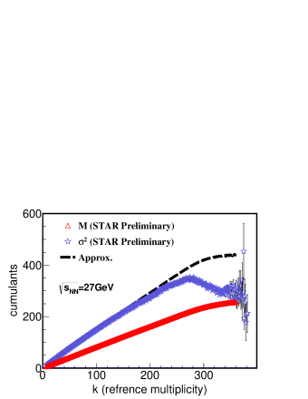
Figure 1: (Color online). Approximate solutions of $\sigma^{2}$ ($c_{2}$) of the total charge multiplicity distribution in Au+Au collisions at $\sqrt{s_{NN}}=27$GeV. The approximate solutions are obtained from Eq.(29). The input distribution $\mathscr{M}(k)$ are taken from Tang (2014).

In Fig. 1, we show the approximate solutions of $\sigma^{2}$ of the total charge multiplicity distribution in Au+Au collisions at $\sqrt{s_{NN}}=27$GeV as function of reference multiplicity $k$. The input distribution $\mathscr{M}(k)$ (open triangle symbol) are taken from Tang (2014). We find that the approximate solution (black-dashed line) can reproduce the experimental results(open star symbol) expect the central collision range. The deviations in most central collision are due to the non-trivial features of $\mathscr{P}_{A}(k)$ in this range, that make the second assumption $\mathscr{P}_{A}(k+m)/\mathscr{P}_{A}(k)\simeq 1$ becomes invalid.

From the approximate solutions, we obtain the relationship among the scale variance of total charge hadrons $\omega_{ch}$, positive hadrons $\omega_{+}$ and negative hadrons $\omega_{-}$

$$\omega_{ch}=\omega_{+}+\omega_{-}-1.$$ (34)

Within the accuracy errors this relations can be used to explain the experiment measurements from NA49 collaborations Alt et al. (2007) and PHENIX collaborations  Adare et al. (2008) surprisingly well, even the effect of resonance decays have not been included in the present study. Moreover, the $M/k$ ratios help to explain the differences on scale variance of total charge distributions measured in different centralities and different experiments Alt et al. (2007); Adare et al. (2008); Tang (2014); Mukherjee (2016).

III.3.1 Net-conserved charges

Analogously, we obtain the approximate solutions of first four cumulants of $\mathscr{P}_{B|A}(n|k)$ as

$$c_{1}^{N} = M_{+}-M_{-},$$ (35)

$$c_{2}^{N} = \frac{(M_{+}-M_{-})^{2}}{k+1}+M_{+}+M_{-},$$ (36)

$$c_{3}^{N} = \frac{2(M_{+}-M_{-})^{3}}{(k+1)^{2}}+\frac{3(M_{+}^{2}-M_{-}^{2})}{k+1}+c_{1}^{N},$$ (37)

$$c_{4}^{N} = \frac{6(M_{+}-M_{-})^{4}}{(k+1)^{3}}+\frac{12(M_{+}-M_{-})^{2}(M_{+}+M_{-})}{(k+1)^{2}}$$ (38)

$$+\frac{6(M_{+}^{2}+M_{-}^{2})}{k+1}+c_{2}^{N},$$

where $M_{+}$ and $M_{-}$ are the mean values of positive and negative conserved charges in a given reference multiplicity bin $k$.

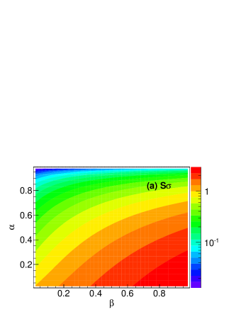
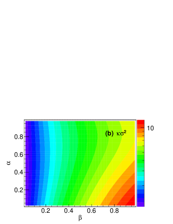
Figure 2: (Color online). The $\beta-\alpha$ plane of $S\sigma$(upper panel) and $\kappa\sigma^{2}$(lower panel) of multiplicity distribution of net-conserved charges. $\beta$ is the multiplicity ratio between positive-conserved charges and the reference multiplicity, $\alpha$ is the multiplicity ratio between negative and positive-conserved charges. For the details, see Eq.(39) and Eq.(40).

Due to less sensitive to the interaction volume and experimental efficiency Karsch and Redlich (2011); Alba et al. (2014); Fu (2013); Aggarwal et al. (2010); Adamczyk et al. (2014a, b), the moment products $S\sigma\equiv c_{3}^{N}/c_{2}^{N}$ and $\kappa\sigma^{2}\equiv c_{4}^{N}/c_{2}^{N}$ have been frequently discussed in both theory and experiment. From the above approximate solutions, we have

$$S\sigma = 2\beta(1-\alpha)+\frac{\beta(1-\alpha^{2})+1-\alpha}{\beta(1-\alpha)^{2}+1+\alpha},$$ (39)

$$\kappa\sigma^{2} = 6\beta(\gamma-\frac{2\alpha}{\gamma})+1,$$ (40)

where $\alpha=M_{-}/M_{+}$, $\beta=M_{+}/(k+1)$ and $\gamma=\beta(1-\alpha)^{2}+1+\alpha$. If $\beta\rightarrow 0$, Eq.(39) and Eq.(40) will back to the Skellam expectations: $S\sigma=(1-\alpha)/(1+\alpha)$ and $\kappa\sigma^{2}=1$.

In Fig. 2 we show the $\beta-\alpha$ plane of $S\sigma$ and $\kappa\sigma^{2}$ from Eq.(39) and Eq.(40). The approximate solutions can explain many observations on multiplicity fluctuations except the most-central and most-peripheral centralities:

1. Centrality resolution effect. The moments and its products $S\sigma$ and $\kappa\sigma^{2}$ not only dependent on the multiplicity ratio between negative and positive conserved charges, but also depend on the multiplicity used for centrality definition. This property has been found in both experimental measurements and some model calculations Luo et al. (2013), which was considered as centrality resolution effect. More specifically, a larger pseudorapidity range of reference multiplicity contribute to a smaller values of $S\sigma$ and $\kappa\sigma^{2}$ due to its smaller $\beta$, and vice versa.

2. Net-charge versus net-kaon. Comparison with the cumulants of net-charges and net-kaons distributions, the $\kappa\sigma^{2}$ of net-charges distributions will be larger than the net-kaons one due to its larger $\beta$ and $\alpha$, see Fig. 2(b). But for $S\sigma$, there is a competition between $\beta$ and $\alpha$, because $S\sigma$ increase with $\beta$ and decrease with $\alpha$, as it was shown in Fig. 2(a). Meanwhile, due to the smaller $\beta$ in net-kaons case, its cumulants will be more closer to the Skellam baseline measure than in the net-charges case. These features are in consist with data Adamczyk et al. (2014b); Sarkar (2014).

3. Independent production approximation. As we have mentioned before, the independent production relations of positive and negative-conserved charges has been violated in event-by-event analysis. Moreover, the NBD baselines obtained by $c_{n}^{N}=c_{n}^{\mu_{+}}+(-1)^{n}c_{n}^{\mu_{-}}$ overestimate the higher order cumulants of net-conserved charges distributions Adamczyk et al. (2014b). However, the corrections for $S\sigma$ and $\kappa\sigma^{2}$ depended on the parameters $\beta$ and $\alpha$.

4. Quantitative estimation. Using $(M_{+}+M_{-})\simeq k\gg(M_{+}-M_{-})$ in the net-charge case Adamczyk et al. (2014b), we have $\beta\simeq 1/(1+\alpha)$, $\alpha\simeq 1$ and

   $$S\sigma \simeq \frac{4(1-\alpha)}{1+\alpha},$$ (41)

   $$\kappa\sigma^{2} \simeq 4,$$ (42)

   which are about four times of the Skellam expectations. The results are shown in Fig. 3 and Fig. 4. We find that the approximate solutions of $S\sigma$ are closer to the experiment data/NBD baselines than the Skellam baselines given in Adamczyk et al. (2014b). The approximate solutions of $\kappa\sigma^{2}$ are colser to the NBD baselines, but fail to quantitatively reproduce the data. This indicate the existence of correlations of positive and negative charges Adamczyk et al. (2014b) and/or the correlations between the moment-analysis parameters and the reference particles. Notice that, though it have been shown in the figures, the approximate solutions in $0-5\%$ and $60-80\%$ centrality bins are questionable due to the non-trivial features of $\mathscr{P}_{A}(k)$ in these ranges.

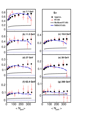
Figure 3: (Color online). Approximate solutions of $S\sigma$ of the net-charge multiplicity distribution in Au+Au collisions at $\sqrt{s_{NN}}=7.7$ to $200$ GeV. The data, Skellam and NBD baselines are taken from  Adamczyk et al. (2014b). The approximate solutions are four times of the Skellam measures, see Eq.(41).

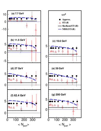
Figure 4: (Color online). Similar to Fig. 3, but for $\kappa\sigma^{2}$. The approximate solutions are four times of the Skellam measures, see Eq.(42).

III.4 Comments and discussion

In this section we have calculated the improved baseline measure of higher order cumulants of multiplicity distribution. We found that, even uner Poisson approximation, the statistical baseline measure deviates from the Poisson measure. However, as we have mentioned, even in a SSE there are some other effects that make the multiplicity fluctuation deviates from Poisson distribution. These corrections should be taken into account especially in the case of $\beta\rightarrow 0$ when the former deviations are small.

In general, the two sub-events used for centrality definition and for moment-analysis are expected to be totally independent of each event. However, the unexpected correlations between them, as well as the correlations between the positive and negative-conserved charges in net-conserved charges case, might contaminate our discussions.

These correlations might be one of the reason why the Binomial distribution instead of NBD have be observed in experiment Adamczyk et al. (2014a) for the protons and anti-protons distributions. We notice that the two sub-events used for centrality definition and for moment analysis share a common pseudorapidity range. Using a transport dynamic model Westfall (2015), the author found that the high order cumulants of net-proton distributions are sensitive to the definition of reference multiplicity. Meanwhile, due to the small $\beta$ in proton and anti-proton cases, some other corrections might overcome the correction discussed in this work, and alter the classifications of proton and anti-proton distributions.

IV Conclusion

The traditional calculations of higher order cumulants of multiplicity distributions are incomplete due to lack of the distribution of principal thermodynamic variables and the probability condition from reference multiplicity. After including the distribution of principal thermodynamic variables, we have derived a general expression for the multiplicity distribution in terms of a conditional probability with arbitrary statistical ensembles and distribution of thermodynamic variables. As an application, we have used the general formula to calculate higher order cumulants under the Poisson approximation.

We found that the improved baseline measure for multiplicity distribution mimics the negative binomial distribution instead of Poisson one, though the Poisson distribution was used as input in a specific statistical ensemble. The deviation of the new baseline measure from the Poisson one increases with the ratio of the mean multiplicity $M$ to the corresponding reference multiplicity $(k+1)$. The basic statistical expectations work well in describing the negative binomial multiplicity distribution measured in experiments, e.g. the cumulants (cumulant products) for multiplicity distribution of total (net) charges.

Similar to the trivial Poisson expectations, the basic statistical expectations can be directly constructed from experiment, but with the data of mean multiplicity $\mathscr{M}(k)$ and distribution of reference multiplicity $\mathscr{P}_{A}(k)$ . However, we note that currently the exact statistical measure cannot be fully determined because of insufficient data. These data are crucial for calculation of the new baseline measure especially in most central collision due to non-trivial feature of $\mathscr{P}_{A}(k)$ in this range. The measurements of these distributions are highly expected in the future to pin down the exact statistical measure.

Appendix A Moments and cumulants

For a probability distribution $f(x)$, the moment-generating function can be written as,

$$M(t)=\int_{-\infty}^{\infty}f(x)e^{tx}dx.$$ (43)

We obtain the sereies expansion,

$$M(t)=\sum_{n=0}^{\infty}m_{n}\frac{t^{n}}{n!},$$ (44)

where $m_{n}$ is the $n$th-order raw moment for $f(x)$

$$m_{n}=\int_{-\infty}^{\infty}dxx^{n}f(x).$$ (45)

The cumulant-generating function is defined as

$$K(t)=\ln M(t)=\sum_{n=1}^{\infty}c_{n}\frac{t^{n}}{n!},$$ (46)

where $c_{n}$ is the $n$th-order cumulant of $f(x)$. Then we have

$$M(t)=\sum_{n=0}^{\infty}m_{n}\frac{t^{n}}{n!}=\exp(\sum_{n=1}^{\infty}c_{n}\frac{t^{n}}{n!}).$$ (47)

By taking $n$th order derivatives at $t=0$, we have

$$m_{n+1} = \sum_{p=0}^{n}\frac{n!}{p!(n-p)!}m_{n-p}c_{p+1},$$ (48)

$$c_{n+1} = m_{n+1}-\sum_{p=0}^{n-1}\frac{n!}{p!(n-p)!}m_{n-p}c_{p+1},$$ (49)

The first four order explicit relation, which was frequently used in this paper, reads,

$$m_{1} = c_{1},$$ (50)

$$m_{2} = c_{2}+c_{1}^{2},$$ (51)

$$m_{3} = c{3}+3c_{1}c_{2}+c_{1}^{3},$$ (52)

$$m_{4} = c_{4}+4c_{3}c_{1}+3c_{2}^{2}+6c_{2}c_{1}^{2}+c_{1}^{4},$$ (53)

and

$$c_{1} = m_{1}\equiv\mu,$$ (54)

$$c_{2} = m_{2}-m_{1}^{2}\equiv\sigma^{2},$$ (55)

$$c_{3} = m_{3}-3m_{2}m_{1}+2m_{1}^{3}\equiv S\sigma^{3},$$ (56)

$$c_{4} = m_{4}-4m_{3}c_{1}-3m_{2}^{2}+12m_{2}m_{1}^{2}-6m_{1}^{4}$$ (57)

$$\equiv \kappa\sigma^{4},$$

where $\mu$, $\sigma^{2}$, $S$ and $\kappa$ are mean value, variance, skewness and kurtosis of probability distribution $f(x)$, respectively.

For the Poisson distribution, we have

$$c_{1}=c_{2}=c_{3}=c_{4}=\lambda,$$ (58)

where $\lambda$ is the Poisson parameter shown in Eq.(9). The scale variance for Poisson distribution is $\omega=c_{2}/c_{1}=1$.

For the NBD, we have

$$c_{1} = \frac{rp}{1-p},$$ (59)

$$c_{2} = \frac{rp}{(1-p)^{2}},$$ (60)

$$c_{3} = \frac{rp(1+p)}{(1-p)^{3}},$$ (61)

$$c_{4} = \frac{6rp^{2}}{(1-p)^{4}}+\frac{rp}{(1-p)^{2}},$$ (62)

where $r$ and $p$ are NBD parameters shown in Eq.(1). The scale variance for NBD is $\omega=c_{2}/c_{1}=1/(1-p)>1$.

References

- Stephanov et al. (1999) Misha A. Stephanov, K. Rajagopal, and Edward V. Shuryak, “Event-by-event fluctuations in heavy ion collisions and the QCD critical point,” Phys.Rev. D60, 114028 (1999).
- Jeon and Koch (1999) S. Jeon and V. Koch, “Fluctuations of particle ratios and the abundance of hadronic resonances,” Phys. Rev. Lett. 83, 5435–5438 (1999).
- Stephanov (2009) M.A. Stephanov, “Non-Gaussian fluctuations near the QCD critical point,” Phys.Rev.Lett. 102, 032301 (2009).
- Bazavov et al. (2012) A. Bazavov et al., “Freeze-out Conditions in Heavy Ion Collisions from QCD Thermodynamics,” Phys. Rev. Lett. 109, 192302 (2012).
- Gupta et al. (2011) Sourendu Gupta, Xiaofeng Luo, Bedangadas Mohanty, Hans Georg Ritter, and Nu Xu, “Scale for the Phase Diagram of Quantum Chromodynamics,” Science 332, 1525–1528 (2011).
- Aggarwal et al. (2010) M.M. Aggarwal et al. (STAR), “Higher Moments of Net-proton Multiplicity Distributions at RHIC,” Phys.Rev.Lett. 105, 022302 (2010).
- Adamczyk et al. (2014a) L. Adamczyk et al. (STAR), “Energy Dependence of Moments of Net-proton Multiplicity Distributions at RHIC,” Phys.Rev.Lett. 112, 032302 (2014a).
- Adler et al. (2007) S. S. Adler et al. (PHENIX), “Measurement of density correlations in pseudorapidity via charged particle multiplicity fluctuations in Au+Au collisions at s(NN)**(1/2) = 200-GeV,” Phys. Rev. C76, 034903 (2007).
- Adare et al. (2008) A. Adare et al. (PHENIX), “Charged hadron multiplicity fluctuations in Au+Au and Cu+Cu collisions from to 200 GeV,” Phys.Rev. C78, 044902 (2008).
- Adamczyk et al. (2014b) L. Adamczyk et al. (STAR), “Beam energy dependence of moments of the net-charge multiplicity distributions in Au+Au collisions at RHIC,” Phys.Rev.Lett. 113, 092301 (2014b).
- Tang (2014) Aihong Tang (STAR), “Beam Energy Dependence of Clan Multiplicity at RHIC,” J.Phys.Conf.Ser. 535, 012009 (2014).
- Adare et al. (2016) A. Adare et al. (PHENIX), “Measurement of higher cumulants of net-charge multiplicity distributions in AuAu collisions at GeV,” Phys. Rev. C93, 011901 (2016).
- Andronic et al. (2006) A. Andronic, P. Braun-Munzinger, and J. Stachel, “Hadron production in central nucleus-nucleus collisions at chemical freeze-out,” Nucl.Phys. A772, 167–199 (2006).
- Cleymans et al. (2005) J. Cleymans, K. Redlich, and L. Turko, “Probability distributions in statistical ensembles with conserved charges,” Phys.Rev. C71, 047902 (2005).
- Begun et al. (2004) V. V. Begun, M. Gazdzicki, Mark I. Gorenstein, and O. S. Zozulya, “Particle number fluctuations in canonical ensemble,” Phys. Rev. C70, 034901 (2004).
- Begun et al. (2007) V. V. Begun, M. Gazdzicki, Mark I. Gorenstein, M. Hauer, V. P. Konchakovski, and B. Lungwitz, “Multiplicity fluctuations in relativistic nuclear collisions: Statistical model versus experimental data,” Phys. Rev. C76, 024902 (2007).
- Garg et al. (2013) P. Garg, D.K. Mishra, P.K. Netrakanti, B. Mohanty, A.K. Mohanty, et al., “Conserved number fluctuations in a hadron resonance gas model,” Phys.Lett. B726, 691–696 (2013).
- Karsch and Redlich (2011) Frithjof Karsch and Krzysztof Redlich, “Probing freeze-out conditions in heavy ion collisions with moments of charge fluctuations,” Phys.Lett. B695, 136–142 (2011).
- Alba et al. (2014) Paolo Alba, Wanda Alberico, Rene Bellwied, Marcus Bluhm, Valentina Mantovani Sarti, et al., “Freeze-out conditions from net-proton and net-charge fluctuations at RHIC,” Phys.Lett. B738, 305–310 (2014).
- Fu (2013) Jinghua Fu, “Higher moments of net-proton multiplicity distributions in heavy ion collisions at chemical freeze-out,” Phys.Lett. B722, 144–150 (2013).
- Bhattacharyya et al. (2015) Abhijit Bhattacharyya, Rajarshi Ray, Subhasis Samanta, and Subrata Sur, “Thermodynamics and fluctuations of conserved charges in a hadron resonance gas model in a finite volume,” Phys. Rev. C91, 041901 (2015).
- Braun-Munzinger et al. (2011) P. Braun-Munzinger, B. Friman, F. Karsch, K. Redlich, and V. Skokov, “Net-proton probability distribution in heavy ion collisions,” Phys. Rev. C84, 064911 (2011).
- Karsch et al. (2016) Frithjof Karsch, Kenji Morita, and Krzysztof Redlich, “Effects of kinematic cuts on net-electric charge fluctuations,” Phys. Rev. C93, 034907 (2016).
- Bzdak et al. (2013) Adam Bzdak, Volker Koch, and Vladimir Skokov, “Baryon number conservation and the cumulants of the net proton distribution,” Phys. Rev. C87, 014901 (2013).
- Alt et al. (2007) C. Alt et al. (NA49), “Centrality and system size dependence of multiplicity fluctuations in nuclear collisions at 158-A/GeV,” Phys.Rev. C75, 064904 (2007).
- Mukherjee (2016) Maitreyee Mukherjee (ALICE), “Event-by-event multiplicity fluctuations in Pb-Pb collisions in ALICE,” in 11th Workshop on Particle Correlations and Femtoscopy (WPCF 2015) Warsaw, Poland, November 3-7, 2015 (2016) arXiv:1603.06824 [hep-ex] .
- Gorenstein and Hauer (2008) M. I. Gorenstein and M. Hauer, “Statistical Ensembles with Fluctuating Extensive Quantities,” Phys. Rev. C78, 041902 (2008).
- Gorenstein and Gazdzicki (2011) M. I. Gorenstein and M. Gazdzicki, “Strongly Intensive Quantities,” Phys. Rev. C84, 014904 (2011).
- Gorenstein and Grebieszkow (2014) Mark I. Gorenstein and Katarzyna Grebieszkow, “Strongly Intensive Measures for Transverse Momentum and Particle Number Fluctuations,” Phys. Rev. C89, 034903 (2014).
- Skokov et al. (2013) V. Skokov, B. Friman, and K. Redlich, “Volume Fluctuations and Higher Order Cumulants of the Net Baryon Number,” Phys. Rev. C88, 034911 (2013).
- Stodolsky (1995) Leo Stodolsky, “Temperature fluctuations in multiparticle production,” Phys. Rev. Lett. 75, 1044–1045 (1995).
- Wilk and Wlodarczyk (2009) Grzegorz Wilk and Zbigniew Wlodarczyk, “Multiplicity fluctuations due to the temperature fluctuations in high-energy nuclear collisions,” Phys. Rev. C79, 054903 (2009).
- Biro et al. (2014) T. S. Biro, G. G. Barnaföldi, and P. Van, “New Entropy Formula with Fluctuating Reservoir,” Physica 417, 215–220 (2014).
- Sarkar (2014) Amal Sarkar (STAR), “Higher-moment measurements of net-kaon, net-charge and net-proton multiplicity distributions at STAR,” Proceedings, 24th International Conference on Ultra-Relativistic Nucleus-Nucleus Collisions (Quark Matter 2014), Nucl. Phys. A931, 796–801 (2014).
- Luo et al. (2013) Xiaofeng Luo, Ji Xu, Bedangadas Mohanty, and Nu Xu, “Volume fluctuation and auto-correlation effects in the moment analysis of net-proton multiplicity distributions in heavy-ion collisions,” J.Phys. G40, 105104 (2013).
- Becattini et al. (1996) F. Becattini, Alberto Giovannini, and S. Lupia, “Multiplicity distributions in a thermodynamical model of hadron production in e+ e- collisions,” Z. Phys. C72, 491–496 (1996).
- Braun-Munzinger et al. (2012) P. Braun-Munzinger, B. Friman, F. Karsch, K. Redlich, and V. Skokov, “Net-charge probability distributions in heavy ion collisions at chemical freeze-out,” Nucl. Phys. A880, 48–64 (2012).
- Arneodo et al. (1987) M. Arneodo et al. (European Muon), “Comparison of Multiplicity Distributions to the Negative Binomial Distribution in Muon - Proton Scattering,” Z.Phys. C35, 335 (1987).
- Adamus et al. (1988) M. Adamus et al. (EHS/NA22), “Phase Space Dependence of the Multiplicity Distribution in and Collisions at 250-GeV/,” Z.Phys. C37, 215 (1988).
- Ansorge et al. (1989) R.E. Ansorge et al. (UA5), “Charged Particle Multiplicity Distributions at 200-GeV and 900-GeV Center-Of-Mass Energy,” Z.Phys. C43, 357 (1989).
- Aamodt et al. (2010) K. Aamodt et al. (ALICE), “Charged-particle multiplicity measurement in proton-proton collisions at and 2.36 TeV with ALICE at LHC,” Eur.Phys.J. C68, 89–108 (2010).
- Khachatryan et al. (2011) Vardan Khachatryan et al. (CMS), “Charged particle multiplicities in interactions at , 2.36, and 7 TeV,” JHEP 1101, 079 (2011).
- Adamczyk et al. (2012) L. Adamczyk et al. (STAR), “Inclusive charged hadron elliptic flow in Au + Au collisions at = 7.7 - 39 GeV,” Phys.Rev. C86, 054908 (2012).
- Xu (2016) Hao-jie Xu, “Cumulants of multiplicity distributions in most central heavy ion collisions,” (2016), arXiv:1602.07089 [nucl-th] .
- Westfall (2015) Gary D. Westfall, “UrQMD Study of the Effects of Centrality Definitions on Higher Moments of Net Protons at RHIC,” Phys. Rev. C92, 024902 (2015).