Test of the universality of free fall with atoms in different spin orientations

Abstract

We report a test of the universality of free fall (UFF) by comparing the gravity acceleration of the ⁸⁷Rb atoms in $m_{F}=+1$ versus that in $m_{F}=-1$, where the corresponding spin orientations are opposite. A Mach-Zehnder-type atom interferometer is exploited to sequentially measure the free fall acceleration of the atoms in these two magnetic sublevels, and the resultant E$\rm{\ddot{o}}$tv$\rm{\ddot{o}}$s ratio is ${\eta_{S}}=(0.2\pm 1.2)\times 10^{-7}$. This also gives an upper limit of $1.1\times 10^{-21}$ GeV/m for possible gradient field of the spacetime torsion. The interferometer using atoms in $m_{F}=\pm 1$ is highly sensitive to the magnetic field inhomogeneity, and a double differential measurement method is developed to alleviate the inhomogeneity influence. Moreover, a proof experiment by modulating the magnetic field is performed, which validates the alleviation of the inhomogeneity influence in our test.

The universality of free fall (UFF) is one of the fundamental hypotheses in the foundation of Einstein's general relativity (GR) Mis73 . Traditional verifications of the UFF are performed with macroscopic bodies that weight differently or comprise different material Su94 ; Gun97 ; Wil04 ; Sch08 ; Nie87 ; Kur89 ; Car92 ; Dic94 , achieved a level of 10^-13 Gun97 ; Wil04 ; Sch08 . There are also lots of work investigating possible violation of UFF that may be induced by spin-related interactions Heh76 ; Pet78 ; Mas00 ; Zha01 ; Sil07 ; Ni10 ; Yas80 ; Sha02 ; Hu12 , and UFF tests of this kind have been performed with polarized or rotating macroscopic bodies Hay89 ; Fal90 ; Nit90 ; Win91 ; Hou01 ; Zhou02 ; Luo02 ; Ni11 ; Obu14 . In this work two kinds of proposed spin-related couplings are concerned, namely spin-gravity coupling and spin-torsion coupling. The corresponding Hamiltonian operators read as Hou01 ; Obu14

$$\left\{\begin{array}[]{l}{H_{{\rm{spin-gravity}}}}=f(r)\vec{S}\cdot\hat{r}\\ {H_{{\rm{spin-torsion}}}}=-c\vec{S}_{\rm{Tor}}\cdot\vec{S}/2\end{array}\right.,$$ (1)

where $\vec{S}$ is the test mass spin, and $\vec{S}_{\rm{Tor}}$ stands for the spacetime torsion. In Eq. (1), $\vec{r}$ points from the earth center to the test mass, $f(r)$ is an arbitrary scalar function of $r$, and $c$ is the light speed. Although UFF tests involving spin-gravity coupling using polarized macroscopic bodies have achieved a precision of 10^-9, the precision decreases dramatically to a level of 10^-5 when the result is re-interpreted in terms of polarized nucleus and even to 10^-3 in terms of polarized electron Ni10 ; Hou01 . This strongly suggests a direct UFF test using microscopic test masses to investigate spin-gravity coupling. On the other hand, for spin-torsion coupling, it is believed that only matter with intrinsic spin could be affected by the spacetime torsion Yas80 ; Obu14 . And in this sense, spinful atoms appear to be natural sensors for the torsion experiments. The spacetime torsion may change along with space, namely torsion gradient exists, about which there is no information. Here this information will be explored using spinful quantum particles.

UFF tests with quantum objects have earlier been performed with a neutron interferometer Col75 , and in recent years, were carried out by comparing the free fall acceleration between different atoms or between atoms and macroscopic masses Pet99 ; Fray04 ; Mer10 ; Poli11 ; Bon13 ; Zhou15 ; Sch10 . Up to date, the best precision using quantum objects is $7\times 10^{-9}$ Pet99 , if the motivations of these tests are not distinguished. UFF tests on quantum basis are still going on Dic13 and tests with higher aimed precision have been proposed Agu14 ; Har15 . As for spin-related UFF tests with quantum objects, there are few experiments performed. In 2004, the difference of the free fall acceleration with atoms in two different hyperfine states has been tested at $1.2\times 10^{-7}$ Fray04 . Tarallo et al. Tar14 performed an UFF test using the bosonic ⁸⁸Sr isotope versus the fermionic ⁸⁷Sr isotope at $1.6\times 10^{-7}$ by Bloch oscillation. In their experiment, the ⁸⁷Sr atoms were in a mixture of different magnetic sublevels, resulting in an effective sublevel of $\left\langle{{m_{F}}}\right\rangle=0$. They also gave an upper limit for spin-gravity coupling by analyzing the resonance linewidth broadening caused by possible different free fall accelerations between different magnetic sublevels. However, we note that possible anomalous spin-spin couplings Win91 ; Chui93 ; Gle08 or dipole-dipole interaction Lah09 between the ⁸⁷Sr atoms with different magnetic sublevels may disturb, or even cover the spin-gravity coupling effects in their experiment. Since most models describing spin-related couplings imply a dependence on the orientation of the spin, we perform a new UFF test with ⁸⁷Rb atoms sequentially prepared in two opposite spin orientations (Fig. 1), namely $m_{F}=+1$ versus $m_{F}=-1$. The corresponding free fall accelerations are compared by atom inteferometry Pet01 ; Bor02 ; Mul08 ; Zhou12 ; Hu13 , which determines the spin-orientation related E$\rm{\ddot{o}}$tv$\rm{\ddot{o}}$s ratio Eot22 as

$${\eta_{S}}\equiv 2({g_{+}}-{g_{-}})/({g_{+}}+{g_{-}}),$$ (2)

where the gravity acceleration of atoms in $m_{F}=+1$ ($m_{F}=-1$) is denoted as $g_{+}$ ($g_{-}$). This provides a direct way to test spin-orientation related UFF on quantum basis. And according to Eq. (1), if the origin of possible violation of UFF is attributed to spin-torsion coupling, torsion gradient can be linked to $\eta_{S}$ as

$${\partial_{z}}{({S_{{\rm{Tor}}}})_{z}}=-\eta_{S}m({g_{+}}+{g_{-}})/c\Delta{S_{z}},$$ (3)

where $m$ is the atom mass, and $\Delta{S_{z}}$ stands for the difference of the spins projection onto vertical direction. Thus through this kind of UFF test, possible torsion gradient can be also probed.

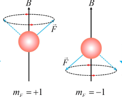
Figure 1: (color online) Schematic of the spin orientations for ⁸⁷Rb atoms in magnetic sublevel $m_{F}=+1$ versus $m_{F}=-1$ of the 5²S_1/2 hyperfine levels. The bias magnetic field $\vec{B}$ defines the external direction to which the atomic spin is referenced. And the total angular momentum $\vec{F}$ of each atom processes around $\vec{B}$.

Compared with UFF tests using polarized or rotating macroscopic masses, it is much easier to prepare atomic ensemble with pure polarization using stimulated Raman transitions Mol92 . However, with atoms in sublevels $m_{F}=\pm 1$, the interferometers are highly sensitive to the magnetic field inhomogeneity. Thus it is necessary to select a relatively homogeneous region for interfering. The magnetic field throughout the shielded interfering tube is mapped Zhou10 ; Hu11 , and the region at about 742 mm height above the magnetic-optical trap (MOT) center is selected out. The magnetic field there varies less than 0.1 mG over several millimeters range in vertical distance with a 115 mG bias magnetic field. Moreover, compensating coils in anti-Helmholtz configuration are utilized to further decrease the inhomogeneity. With an injection current of 110 $\rm\mu$A for the compensating coils, the inhomogeneity is decreased by about one order of magnitude. But the magnetic field shows a binomial variation along with the vertical distance. The phase shift induced by the magnetic field inhomogeneity can be calculated by ${\varphi_{B}}=2{\alpha}[\int_{0}^{T}{B(z(t))dt}-\int_{T}^{2T}{B(z(t))dt}]$ Pet99 ; Zhou10 ; Hu11 ; Dav08 , where $\alpha$ is the strength of first-order Zeeman shift for ⁸⁷Rb atoms in 5${}^{2}{\rm S}_{1/2}$ state, $B(z(t))$ denotes the magnetic field at $z(t)$, and $T$ is the separation time between Raman laser pulses. Considering a binomial variation model of $B(z(t))=B({z_{0}})+{\gamma_{1}}(z(t)-{z_{0}})+{\gamma_{2}}{(z(t)-{z_{0}})^{2}}/2$ (here $\gamma_{1}$ ($\gamma_{2}$) is the first (second) order inhomogeneity coefficient, and $z_{0}$ stands for an arbitrary reference point in the selected region), the phase shift induced by the gravity acceleration and the magnetic field gradient is expressed as

$$\varphi_{{m_{F}}}^{\pm}=\mp{k_{{\rm{eff}}}}{g_{{m_{F}}}}T_{{\rm{eff}}}^{2}+2{\alpha}{m_{F}}{T^{2}}({V_{\pi}}\mp{V_{\rm r}}/2)[{\gamma_{1}}+{\gamma_{2}}({V_{\pi}}+gT/4\mp{V_{\rm r}}/2)T+{\gamma_{2}}(z_{\rm{s}}-z_{0})],$$ (4)

where the superscript $\pm$ denotes the corresponding direction of $\emph{{k}}_{\rm{eff}}$ in the interfering process, with $+$ ($-$) indicating the same (opposite) direction between $\emph{{k}}_{\rm{eff}}$ and local gravity acceleration. And ${T_{{\rm{eff}}}}\equiv T\sqrt{1+2\tau/T+4\tau/\pi T+8{\tau^{2}}/\pi{T^{2}}}$ is the effective separation time accounting for the effect of finite Raman pulses duration ( $\tau$ is the duration of the $\pi/2$ Raman pulse) Li15 . In Eq.(4), the second term corresponds to the effect that induced by the magnetic field inhomogeneity, where $V_{\rm r}$ is the recoil velocity, $V_{\pi}$ is the average vertical velocity of the atoms in $F=1$ at the moment of the interfering $\pi$ pulse (the atoms are initially prepared in $F=1$ before the interfering), and $z_{\rm s}$ is the site where the interfering process begins.

According to Eq. (4), we take three steps to alleviate the influence of the magnetic field inhomogeneity in this work. Firstly, the atomic fountain apex is set near the selected interfering region. Actually, the time of the interfering $\pi$ pulse is only about 3 ms near the apex time here. We find this approach is effective to improve our WEP test. On one hand, with this quasi-symmetrical trajectory for atoms, the influence of the magnetic field inhomogeneity cancels significantly. This cancelation assures a relatively long interrogation time (a separation time as large as $T=25$ ms is allowed here, quite larger than $T=1$ ms in Zhou10 ; Hu11 ), which effectively enlarges the signal of the gravity acceleration. On the other hand, near the fountain apex, the center of the atomic cloud only moves by a 4.2 mm vertical distance during the interfering process. In such a small region, a binomial model for the magnetic field inhomogeneity is appropriate, which validates the following systematic error correction. Secondly, as already adopted in typical atom gravimeters Pet01 , the direction of the effective Raman laser wave vector $\emph{{k}}_{\rm{eff}}$ is reversed to make a differential measurement for each $m_{F}$. From this reversing $\emph{{k}}_{\rm{eff}}$ method, a differential mode measurement result ($\Delta\varphi_{{m_{F}}}^{\rm d}\equiv(\Delta\varphi_{{m_{F}}}^{+}-\Delta\varphi_{{m_{F}}}^{-})/2$) and a common mode measurement result ($\Delta\varphi_{{m_{F}}}^{\rm c}\equiv(\Delta\varphi_{{m_{F}}}^{+}+\Delta\varphi_{{m_{F}}}^{-})/2$) can be obtained. There is a residual influence of the magnetic field inhomogeneity in $\Delta\varphi_{{m_{F}}}^{\rm d}$ due to the opposite directions of the recoil velocities between $+k_{{\rm{eff}}}$ and $-k_{{\rm{eff}}}$ configurations. With only first order magnetic field inhomogeneity considered, this residual effect can be corrected using $\gamma_{1}$ estimated from $\Delta\varphi_{{m_{F}}}^{\rm c}$. For a binomial inhomogeneity, more information is required to perform the correction. In this work, for each $m_{F}$, a further differential measurement is performed by modulating $V_{\pi}$ between two values (denoted as $V_{\pi}^{I}$ and $V_{\pi}^{II}$). We find that the systematic error correction is simplest by setting $V_{\pi}^{II}=-V_{\pi}^{I}\equiv-V_{\pi}^{0}$. Through the double differential measurement, four combined measurement results can be obtained. The explicit expressions for $\Delta\Phi_{{m_{F}}}^{\rm dc}\equiv(\Delta\varphi_{{m_{F}}}^{\rm{d}}[V_{\pi}^{I}]+\Delta\varphi_{{m_{F}}}^{\rm d}[V_{\pi}^{II}])/2$ and $\Delta\Phi_{{m_{F}}}^{\rm cd}\equiv(\Delta\varphi_{{m_{F}}}^{\rm c}[V_{\pi}^{I}]-\Delta\varphi_{{m_{F}}}^{\rm c}[V_{\pi}^{II}])/2$ are respectively

$$\left\{\begin{array}[]{l}\Delta\Phi_{{m_{F}}}^{\rm dc}=-{k_{{\rm{eff}}}}{g_{{m_{F}}}}T_{{\rm{eff}}}^{2}-{\alpha}{m_{F}}{T^{2}}{V_{\rm r}}[{\gamma_{1}}+{\gamma_{2}}({V_{\pi}^{0}+gT/4})T]\\ \Delta\Phi_{{m_{F}}}^{\rm cd}=2{\alpha}{m_{F}}{T^{2}}{V_{\pi}^{0}}[{\gamma_{1}}+{\gamma_{2}}({V_{\pi}^{0}+gT/4})T]\end{array}\right..$$ (5)

We note that in the deduction of Eq. (5) from Eq. (4), $z_{s}$ varies as $V_{\pi}$. According to Eq. (5), the residual influence of the magnetic field inhomogeneity in $\Delta\Phi_{{m_{F}}}^{\rm dc}$ can be corrected as $\Delta\Phi_{{m_{F}}}^{\rm dc}+\Delta\Phi_{{m_{F}}}^{\rm cd}\times({V_{\rm r}}/2{V_{\pi}^{0}})$, which needs not the knowledge of $\gamma_{1}$ and $\gamma_{2}$. Certainly, with the help of other combined results of the double differential measurement, $\gamma_{1}$ and $\gamma_{2}$ can be estimated.

In the reversing $\emph{{k}}_{\rm{eff}}$ differential measurement, it is important to prepare the atomic ensembles in the same average velocity between the $+k_{{\rm{eff}}}$ and $-k_{{\rm{eff}}}$ configurations for each $m_{F}$, namely $V_{\rm s}^{+}=V_{\rm s}^{-}$ ($V_{\rm s}$ denotes the average velocity of the atomic ensemble after the state preparation, and the superscript $\pm$ denotes the $\emph{{k}}_{\rm{eff}}$ configuration). Thus the atomic ensembles experience the same magnetic field inhomogeneity in the modulation of $\emph{{k}}_{\rm{eff}}$, ensuring a perfect differential measurement. Using conventional state preparation method Mol92 ; Lou11 , the equality strongly depends on the pre-determined Zeeman shift and AC-Stark shift, etc. And the variations of these shifts will cause opposite changes for $V_{\rm s}^{+}$ and $V_{\rm s}^{-}$. Here we explore an easy but reliable method to guarantee this equality. For the two interfering configurations, we implement the state preparations using the Raman lasers both configured in $+k_{\rm{eff}}$ with the same Raman lasers effective frequency $\omega_{{\rm{eff}}}$. In this case, for each $m_{F}$, the state preparations are completely the same for the two interfering configurations. Compared with conventional operation of the interferometer, in addition to usual Raman lasers frequency chirp, this method needs an extra shift of $\omega_{{\rm{eff}}}$ after the state preparation. This shift will switch the Raman lasers configuration from $+k_{\rm{eff}}$ to $-k_{\rm{eff}}$ for the interfering process when needed. As for the modulation of $V_{\pi}$, the state preparation procedures are totally the same. And a delay time of about $2V_{\pi}^{0}/g$ ($g\sim 9.79$ m/s²) is inserted in the timing sequence between the state preparation and the interfering for $V_{\pi}^{II}$, which ensures $V_{\pi}^{II}=-V_{\pi}^{I}$.

The experiment is performed in an atom gravimeter detailedly reported in Ref. Zhou12 . It takes 750 ms to load about 10⁸ cold ⁸⁷Rb atoms from a dispenser using a typical MOT. Then the atoms are launched upward and further cooled to about 7 ${\rm\mu}$K with a moving molasses procedure in the atomic fountain. After a flight time of 356 ms from the launch, a Raman $\pi$ pulse with a duration of 46 $\rm\mu$s is employed to implement the state preparation. Then the unwanted atoms are removed by a blow-away beam. When arriving at 742 mm height, the atomic cloud undergoes the $\pi/2-\pi-\pi/2$ Raman pulses with a pulse separation time of $T=25$ ms. The transition probability of the atoms after the interfering is obtained through normalized fluorescence detection. The entire process of a single shot measurement as described above takes 1.5 s. Before the formal data acquisition, $V_{\pi}^{I,II}$ should be measured for each $m_{F}$ to calculate the correction. This velocity is obtained from the spectroscopy of the VSRT Mol92 with a Raman $\pi$ pulse applied at the right moment. The measured average velocities are $V_{\pi}^{I}=30.6(1)$ mm/s and $V_{\pi}^{II}=-30.6(1)$ mm/s for the selected atoms in both $\left|{F=1,{m_{F}}=+1}\right\rangle$ and $\left|{F=1,{m_{F}}=-1}\right\rangle$ (it takes about 180 s to measure one average velocity. In reality, these velocities will change in long term, which will be discussed later).

Finally, the measurement of the gravity acceleration of the atoms in different magnetic sublevels is performed sequentially. For each $m_{F}$, one full interferometry fringe is obtained by scanning the chirp rate of $\omega_{{\rm{eff}}}$ in 20 steps in each $\emph{{k}}_{\rm{eff}}$ configuration for each $V_{\pi}$, namely 30 s for a full fringe. Meanwhile, in order to reduce the effect of possible long-term drift, eight adjacent fringes are grouped as a cycle unit, with one fringe corresponding to one combination of $\emph{{k}}_{\rm{eff}}$, $V_{\pi}$ and $m_{F}$. The switches between the combinations are automatically controlled by the computer. It takes 10 hours to repeat the cycle unit for 150 times, and the phase shifts are extracted by the cosine fitting from the fringes. The Allan deviation calculated from the consecutive measurement of $\Delta\Phi_{{m_{F}}}^{\rm dc}$ shows a short-term sensitivity of about 3.5$\times 10^{-6}g$/$\sqrt{\rm{Hz}}$ for the gravity acceleration measurement with each $m_{F}$.

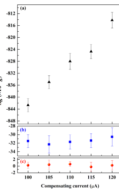
Figure 2: (color online) Estimated $\Delta g$ using different methods in the modulation of the injection current for the compensating coils. The data acquiring time for each injection current is only one hour. In figure (a) no measures are taken to decrease the magnetic field inhomogeneity influence; In figure (b) the conventional differential measurement is adopted to decrease the influence, and in figure (c) the influence is alleviated using the double differential measurement. We note that the error bars in these figures only refer to the statistics standard deviation.

In order to validate the efficiency of alleviating the influence of the magnetic field inhomogeneity in our WEP test by this double differential measurement, in addition to the 110 $\rm\mu$A injection current for the compensating coils, tests with other four values of the current are also performed. And the result is shown in Fig. 2, which is reported as $\Delta g\equiv{g_{+}}-{g_{-}}$ for each injection current (the error bars are only the corresponding statistical standard deviations). In Fig. 2(a), $\Delta g$ is estimated by $\Delta g=(\Delta\varphi_{{m_{F}}=+1}^{+}-\Delta\varphi_{{m_{F}}=-1}^{+})/{k_{\rm{eff}}}T_{\rm{eff}}^{2}$, namely the situation without any differential measurement to decrease the inhomogeneity influence. In Fig. 2(b), $\Delta g$ is estimated by

$$\Delta g=\frac{1}{{{k_{\rm{eff}}}T_{\rm{eff}}^{2}}}[(\Delta\varphi_{{m_{F}}=+1}^{\rm d}+\frac{{{V_{\rm r}}}}{{2V_{\pi}^{0}}}\Delta\varphi_{{m_{F}}=+1}^{\rm c})-(\Delta\varphi_{{m_{F}}=-1}^{\rm d}+\frac{{{V_{\rm r}}}}{{2V_{\pi}^{0}}}\Delta\varphi_{{m_{F}}=-1}^{\rm c})],$$ (6)

which is only capable of eliminating the effect of the first order magnetic field inhomogeneity. And in Fig. 2(c), $\Delta g$ is estimated by

$$\Delta g=\frac{1}{{{k_{\rm{eff}}}T_{\rm{eff}}^{2}}}[(\Delta\Phi_{{m_{F}}=+1}^{\rm dc}+\frac{{{V_{\rm r}}}}{{2V_{\pi}^{0}}}\Delta\Phi_{{m_{F}}=+1}^{\rm cd})-(\Delta\Phi_{{m_{F}}=-1}^{\rm dc}+\frac{{{V_{\rm r}}}}{{2V_{\pi}^{0}}}\Delta\Phi_{{m_{F}}=-1}^{\rm cd})].$$ (7)

According to Fig. 2(a) , the influence of the magnetic field inhomogeneity changes dominantly with the injected current. In Fig. 2(b), the influence of the inhomogeneity has been suppressed by about a factor of 26, but there is still a considerable residual effect. In Fig. 2(c), there is no obvious dependence of $\Delta g$ on the injection current. And what is more important, the residual effect is also suppressed below the level of $10^{-7}g$, which proofs that our correction based on this double differential measurement is quite effective. The statistics result for the 110 $\rm\mu$A compensating current with the 10 hours measurement time is $(-1\pm 3)\times 10^{-8}g$ without any other corrections. It also shows that a majority of the phase shift due to the magnetic field inhomogeneity is canceled in the double differential measurement. The residual effect due to the Raman pulses durations is thus safely neglected here.

In this differential measurement of the gravity acceleration, some disturbances, for example, that are induced by the AC-Stark shift, can be largely suppressed, and other disturbances, for example, that are induced by nearby masses or tilt of the Raman lasers, are common for the atoms in $m_{F}=+1$ and $m_{F}=-1$ and are cancelled in the final comparison. The main systematic error still comes from the effect associated with the magnetic field inhomogeneity. In this work the equality of $V_{\rm s}^{+}$ and $V_{\rm s}^{-}$ is well guaranteed by our special state preparation. However the value of $V_{\rm s}^{+}$ and $V_{\rm s}^{-}$ drifts in a common way due to the change of the AC-Stark shift, which is induced by the variation of the Raman laser power as the room temperature changes periodically. A peak-to-peak variation of 0.25 mm/s for $V_{\pi}$ is observed, which on one hand affects the cancelation in the double differential measurement and on the other hand limits the accuracy of the correction $\Delta\Phi_{{m_{F}}}^{\rm dc}+\Delta\Phi_{{m_{F}}}^{\rm cd}\times({V_{\rm r}}/2{V_{\pi}^{0}})$. The corresponding contributed uncertainty on $\Delta g$ is $1.2\times 10^{-7}g$. We notice that there is a difference of $2\pi\times 2.8$ kHz/G for $\alpha$ between ⁸⁷Rb atoms in $F=1$ versus $F=2$, and the corresponding error is about $-3\times 10^{-8}g$. Though the magnetic field inhomogeneity in the selected interfering region shows a binomial variation, higher order inhomogeneity has been investigated as well. We extent the calculation of Eq. (4) to the case of a third order magnetic field inhomogeneity present, and find our double differential measurement capable to alleviate the influence of the third order inhomogeneity by amount of 70 percent. The final resultant E$\rm{\ddot{o}}$tv$\rm{\ddot{o}}$s ratio (calculated by $\Delta g/g$) is $(0.2\pm 1.2)\times 10^{-7}$, which indicates that the violation of UFF has not been observed at the level of $1.2\times 10^{-7}$ for the atoms with different polarization orientations. According to Eq. (3), this corresponds to a constrain of $1.1\times 10^{-21}$ GeV/m for possible gradient field of spacetime torsion (for this experiment, $\Delta{S_{z}}$ is 2$\left|{{m_{F}}}\right|\hbar$). We note that the bias magnetic field direction is crucial in the deduction of this constrain, since it defines the reference of the spin orientation.

In conclusion, we have tested UFF with atoms in different spin orientations based on a Mach-Zehnder-type atom interferometer, and the violation of UFF is not observed at the level of $1.2\times 10^{-7}$. This work represents the first direct spin-orientation related UFF test on quantum basis, and possible spacetime torsion gradient is also constrained to an upper limit of $1.1\times 10^{-21}$ GeV/m. We anticipate that the precision of this kind of UFF test will be improved by constructing a more homogeneous magnetic field or by exploiting internal-state invariant atom interferometers (see Ref. Fray04 ; Dav08 ; Lev09 ; Berg15 ; Alt13 , for example). In this work, in order to achieve this precision, on one hand, the fountain apex is set near the selected interfering region, and on the other hand, the double differential measurement method as well as the special state preparation method is developed. These strategies may be illuminating for other high precision measurements using atom interferometry.

We thank Yuanzhong Zhang for discussions about the UFF background, Weitou Ni for discussions about UFF tests with macroscopic polarized bodies, Xiangsong Chen, Jianwei Cui and Yungui Gong for discussions about spin-torsion coupling, and Zhifang Xu for discussions about dipole-dipole interaction between atoms. This work is supported by the National Natural Science Foundation of China (Grants Nos. 41127002, 11574099, and 11474115) and the National Basic Research Program of China (Grant No. 2010CB832806).

References

- (1) C. Misner, K. Thorne, and J. Wheeler, Gravitation (Freeman, San Francisco, 1973).
- (2) Y. Su, B. R. Heckel, E. G. Adelberger, J. H. Gundlach, M. Harris, G. L. Smith, and H. E. Swanson, Phys. Rev. D 50, 3614 (1994).
- (3) T. M. Niebauer, M. P. McHugh, and J. E. Faller, Phys. Rev. Lett. 59, 609 (1987).
- (4) K. Kuroda and N. Mio, Phys. Rev. Lett. 62, 1941 (1989).
- (5) S. Carusotto, V. Cavasinni, A. Mordacci, F. Perrone, E. Polacco, E. Iacopini, and G. Stefanini, Phys. Rev. Lett. 69, 1722 (1992).
- (6) J. O. Dickey, P. L. Bender, J. E. Faller et al., Science 265, 482 (1994).
- (7) J. H. Gundlach, G. L. Smith, E. G. Adleberger, B. R. Heckel, and H. E. Swanson, Phys. Rev. Lett. 78, 2523 (1997).
- (8) J. G. Williams, S. G. Turyshev, and D. H. Boggs, Phys. Rev. Lett. 93, 261101 (2004).
- (9) S. Schlamminger, K.-Y. Choi, T. A. Wagner, J. H. Gundlach, and E. G. Adelberger, Phys. Rev. Lett. 100, 041101 (2008).
- (10) F. W. Hehl, P. von der Heyde, G. D. Kerlick, and J. M. Nester, Rev. Mod. Phys. 48, 393 (1976).
- (11) A. Peters, Phys. Rev. D 18, 2739 (1978).
- (12) B. Mashhoon, Class. Quantum Grav. 17, 2399 (2000).
- (13) Y. Z. Zhang, J. Luo, and Y. X. Nie, Mod. Phys. Lett. A 16, 789 (2001).
- (14) A. J. Silenko, O. V. Teryaev, Phys. Rev. D 76, 061101(R) (2007).
- (15) W. T. Ni, Rep. Prog. Phys. 73, 056901 (2010).
- (16) P. B. Yasskin and W. R. Stoeger, Phys. Rev. D 21, 2081 (1980).
- (17) I. L. Shapiro, PHys. Rep. 357, 113 (2002).
- (18) Z. K. Hu, Y. Ke, X. B. Deng, Z. B. Zhou, and J. Luo, Chin. Phys. Lett. 29, 080401 (2012).
- (19) H. Hayasaka and S. Takeuchi, Phys. Rev. Lett. 63, 2701 (1989).
- (20) J. E. Faller, W. J. Hollander, P. G. Nelson, and M. P. Mchugh, Phys. Rev. Lett. 64,825 (1990).
- (21) J. M. Nitschke and P. A. Wilmarth, Phys. Rev. Lett. 64, 2115 (1990).
- (22) D. J. Wineland, J. J. Bollinger, D. J. Heinzen, W. M. Itano, and M. G. Raizen, Phys. Rev. Lett. 67, 1735 (1991).
- (23) L. S. Hou and W. T. Ni, Mod. Phys. Lett. A 16, 763 (2001).
- (24) Z. B. Zhou, J. Luo, Q. Yan, Z. G. Wu, Y. Z. Zhang, and Y. X. Nie, Phys. Rev. D 66, 022002 (2002).
- (25) J. Luo, Y. X. Nie, Y. Z. Zhang, and Z. B. Zhou, Phys. Rev. D 65, 042005 (2002).
- (26) W. T. Ni, Phys. Rev. Lett. 107, 051103 (2011).
- (27) Y. N. Obukhov, A. J. Silenko, and O. V. Teryaev, Phys. Rev. D 90, 124068 (2014).
- (28) R. Colella, A. W. Overhauser, and S. A. Werner, Phys. Rev. Lett. 34, 1472 (1975).
- (29) A. Peters, K. Y. Chung, and S. Chu, Nature (London) 400, 849 (1999).
- (30) S. Fray, C. A. Diez, T. W. Hnsch, and M. Weitz, Phys. Rev. Lett. 93, 240404 (2004).
- (31) S. Merlet, Q. Bodart, N. Malossi, A. Landragin, F. Pereira Dos Santos, O. Gitlein, and L. Timmen, Metrologia 47, L9-L11 (2010).
- (32) N. Poli, F.-Y. Wang, M. G. Tarallo, A. Alberti, M. Prevedelli, and G. M. Tino, Phys. Rev. Lett 106, 038501 (2011).
- (33) A. Bonnin, N. Zahzam, Y. Bidel, and A. Bresson, Phys. Rev. A 88, 043615 (2013).
- (34) D. Schlippert, J. Hartwig, H. Albers et al., Phys. Rev. Lett. 112, 203002 (2014).
- (35) L. Zhou, S. Long, B. Tang, et al., Phys. Rev. Lett. 115, 013004 (2015).
- (36) S. M. Dickerson, J. M. Hogan, A. Sugarbaker, D. M. S. Johnson, and M. A. Kasevich, Phys. Rev. Lett. 111, 083001 (2013).
- (37) D. Aguilera, H. Ahlers, B. Batterlier, et al., Class. Quantum Grav. 31, 159502 (2014).
- (38) J. Hartwig, S. Abend, C. Schubert, et al., New J. Phys. 17, 035011 (2015).
- (39) M. G. Tarallo, T. Mazzoni, N. Poli, D. V. Sutyrin, X. Zhang, and G. M. Tino, Phys. Rev. Lett. 113, 023005 (2014).
- (40) T. C. P. Chui and W. T. Ni, Phys. Rev. Lett. 71, 3247 (1993).
- (41) A. G. Glenday, C. E. Cramer, D. F. Phillips, and R. L. Walsworth, Phys. Rev. Lett. 101, 261801 (2008).
- (42) T. Lahaye, C. Menotti, L. Santos, M. Lewenstein, and T. Pfau, Rep. Prog. Phys. 72, 126401 (2009).
- (43) A. Peters, K. Y. Chung and S. Chu, Metrologia 38, 25 (2001).
- (44) Ch. J. Bordé, Metrologia 39, 435 (2002).
- (45) H. Müller, S. Chiow, S. Herrmann, and S. Chu, Phys. Rev. Lett. 100, 031101 (2008).
- (46) M. K. Zhou, Z. K. Hu, X. C. Duan, B. L. Sun, L. L. Chen, Q. Z. Zhang, and J. Luo, Phys. Rev. A 86, 043630 (2012).
- (47) Z. K. Hu, B. L. Sun, X. C. Duan, M. K. Zhou, L. L. Chen, S. Zhan, Q. Z. Zhang, and J. Luo, Phys. Rev. A 88, 043610 (2013).
- (48) R. Etvs, V. Pekár, and E. Fekete, Ann. Phys. (Leipzig) 68, 11 (1922).
- (49) K. Moler, D. S. Weiss, M. Kasevich, and S. Chu, Phys. Rev. A 45, 342 (1992).
- (50) M. K. Zhou, Z. K. Hu, X. C. Duan, B. L. Sun, J. B. Zhao, and J. Luo, Phys. Rev. A 82, 061602(R) (2010).
- (51) Z. K. Hu, X. C. Duan, M. K. Zhou, B. L. Sun, J. B. Zhao, M. M. Huang, and J. Luo, Phys. Rev. A 84, 013620 (2011).
- (52) J. P. Davis and F. A. Narducci, Journal of Modern Optics 55, 3173 (2008).
- (53) X. Li, C. G. Shao, and Z. K. Hu, J. Opt. Soc. Am. B 32, 248 (2015).
- (54) A. Louchet-Chauvet, T. Farah, Q. Bodart, A. Clairon, A. Landragin, S. Merlet, and F. P. Dos Santos, New J. Phys. 13, 065025 (2011).
- (55) T. Lévèque, A. Gauguet, F. Michaud, F. Pereira Dos Santos, and A. Landragin, Phys. Rev. Lett. 103, 080405 (2009).
- (56) P. Berg, S. Abend, G. Tackmann, C. Schubert, E. Giese, W. P. Schleich, F. A. Narducci, W. Ertmer, and E. M. Rasel, Phys. Rev. Lett. 114, 063002 (2015).
- (57) P. A. Altin, M. T. Johnsson, V. Negnevitsky, et al., New J. Phys. 15, 023009 (2013).