Unidirectional transport of wave packets through tilted discrete breathers in nonlinear lattices with asymmetric defects

Abstract

We consider the transfer of lattice wave packets through a tilted discrete breather (TDB) in opposite directions in the discrete nonlinear Schrödinger model with asymmetric defects, which may be realized as a Bose-Einstein condensate trapped in a deep optical lattice, or as optical beams in a waveguide array. A unidirectional transport mode is found, in which the incident wave packets, whose energy belongs to a certain interval between full reflection and full passage regions, pass the TDB only in one direction, while, in the absence of the TDB, the same lattice admits bi-directional propagation. The operation of this mode is accurately explained by an analytical consideration of the respective energy barriers. The results suggest that the TDB may emulate the unidirectional propagation of atomic and optical beams in various settings. In the case of the passage of the incident wave packet, the scattering TDB typically shifts by one lattice unit in the direction from which the wave packet arrives, which is an example of the tractor-beam effect, provided by the same system, in addition to the rectification of incident waves.

Keywords: Discrete localized modes, Discrete nonlinear Schrödinger (DNLS) equation, Unidirectional transport, Wave packets, Diode effect

I Introduction

Time-periodic spatially localized excitations, called discrete breathers (DBs) AJSievers1998 ; SFlach1998 ; Panos , are supported by diverse nonlinear lattice media, such as arrays of micromechanical cantilevers MSato2006 , coupled Josephson junctions ETrias2000 ; AVUstinov2003 and optical waveguides DNChr ; RMorandotti1999 ; HSEisenberg1998 ; Kobelke (in the latter case, the evolution variable is not time but the propagation distance), antiferromagnets UTSchwarz1999 ; MSato2004 , Bose-Einstein condensates (BECs) ATrombettoni2001 ; BEiermann2004 ; Konotop and Tonks-Girardeau Kolomeisky1992 or superfluid fermionic JuKuiXue2008 gases fragmented and trapped in deep optical lattices (OLs), as well as some dissipative systems MGClerc2011 ; PCMatthews2011 . DBs provide means for energy concentration and transport in waveguides SFlach1998 , polaronic materials JDAndersen1993 , long biological molecules MPeyrard1993 , and other settings Panos .

DBs may represent attractors in dissipative systems SFlach1998 ; PJMartinez2003 ; RSMacKay1998 and self-trapped localized stationary modes in conservative nonlinear lattices GPTsironis1996 ; RLivi2006 ; GSNg2009 (we keep acronym DB in those stationary states too, although a more appropriate name for them may be merely discrete solitons, as they do not feature breathing dynamics). Collisions of moving solitons or phonons (linear wave packets) with stationary DBs were studied too RLivi2006 ; GSNg2009 ; RFranzosi2007 ; XDBai2012 . It was found that, if the amplitude of the incident soliton is too small, it bounces back from the DB. Beyond a specific threshold amplitude, a part of the norm of the incident solitary pulse may be transmitted through the DB. In particular, this transport property is vital for matter-wave interferometry TSchumm2005 and quantum-information processing DJaksch1999 ; GKBrennen1999 ; JKPachos2003 ; A.Kay2006 .

Previous works were mainly dealing with symmetric DBs in perfect lattices, the corresponding transfer mechanism being symmetric with respect to the direction of motion of the incident excitation. On the other hand, unidirectional propagation of waves in specially devised systems has drawn much attention too (see Ref. Lepri , and references therein). In particular, it was experimentally demonstrated that a periodically poled waveguide may serve as an optical diode Assanto . Further, it was predicted that a combination of a Bragg grating with a periodic lattice built of gain and loss elements Bragg-uni , as well as a periodically structured metamaterial meta , a chain of driven ultracold atoms atomic-chain-uni , and chains of coupled microcavities Fabio may give rise to nonreciprocal light transmission. Starting from early work Scalora , it was also demonstrated theoretically that photonic crystals (PCs) with edge modes Ablowitz , PCs with built-in periodic lattices of defects PhotCryst-uni , second-harmonic-generating PCs VKVK , and quasiperiodic PCs Fabio2 , may produce a similar effect. Other theoretically predicted and experimentally realized possibilities for the unidirectional light transmission are offered by $\mathcal{PT}$-symmetric photonic lattices PT-uni . Asymmetric propagation of microwaves micro-uni and electric signals electric-uni was observed, respectively, in appropriately built electromagnetic crystals and electric transmission lines.

Realistic lattices always contain imperfections (defects). In many cases, they dramatically affect the properties of lattices carrying onsite nonlinearities, resulting in a number of new phenomena, such as Anderson localization PWAnderson1958 ; JBilly2008 , intraband discrete breathers GKopidakis2000 , and the disorder-induced Bose-glass phase LFallani2007 . The influence of disorder on the lattice transport was widely investigated too. It was demonstrated, in various settings, that the interplay of the disorder with self-defocusing nonlinearity may replace the localization by subdiffusion AIomin2010 . More subtle dynamical regimes, represented by infinite-dimensional Kolmogorov-Arnold-Moser tori, are possible too MJohansson2010 .

Unlike those works, our subject here is modification of the lattice transport by DBs pinned to local defects. In particular, if defects have an asymmetric shape, they asymmetrically deform pinned lattice solitons (alias discrete breathers) GKopidakis2000 , making them tilted discrete breathers (TDBs). In this work, we consider a one-dimensional discrete nonlinear Schrödinger (DNLS) model with asymmetric defects and demonstrate that, while the underlying lattice admits bidirectional transmission of linear waves, the transmission may be made nonreciprocal for waves hitting a pinned TDB from opposite directions. As a result, we find a “diodelike” transport mode, where the incident wave packets can pass through the TDB only in one direction, provided that the packet’s energy falls into an appropriate interval between cases of full reflection and full passage (for small and large energies, respectively). Thus, while a localized asymmetric defect cannot directly induce the unidirectional transmission, it may create such a regime with the help of the pinned TDB. This is possible because the scattering of waves on a soliton in a nonlinear system is essentially different from the scattering on a defect in the linear counterpart of the same system. In particular, the nonlinearity gives rise to the interaction of the wave with its own complex-conjugate counterpart, which does not happen in the linear limit. The diode mode can be controlled by varying parameters of the underlying defect, as well as the amplitude (i.e., energy) of the pinned TDB.

The paper is organized as follows. In Sec. II, we introduce the model and produce tilted discrete breathers for dilute gases of bosonic atoms trapped in the deep OL. Unidirectional transport of wave packets through the TDBs is reported in Sec. III. Conclusions are presented in Sec. IV. Additional technical details and limit cases are presented in the Appendix.

II The model and tilted discrete breathers

We start by taking the Bose-Hubbard Hamiltonian, which is the basic model that captures the dynamics of a dilute gas of bosonic atoms in the deep OL. In the mean-field approximation, the Hamiltonian for the disordered OL is ZYSun2015 ; DJaksch1998

$$\mathcal{H}\!=\!\sum_{n=1}^{M}\left(\frac{U}{2}|\psi_{n}|^{4}\!+\!\varepsilon_{n}|\psi_{n}|^{2}\right)-\!\frac{J}{2}\!\sum_{n=1}^{M-1}\!\left(\psi_{n}^{\ast}\psi_{n+1}\!+\mathrm{c.c.}\right),$$ (1)

where $n$ $=1,\ldots,M$ is the discrete coordinate of lattice sites, $\psi_{n}$ is the on-site wave function, $J$ is the amplitude of the inter-site hopping, and c.c. stands for the complex conjugate. Further, $U=4\pi\hbar^{2}a_{s}V_{d}/m$ is the strength of the collisional on-site interactions, where $V_{d}$ is the effective mode volume of each site, $m$ is the atomic mass, and $a_{s}$ is the s-wave atomic scattering length. We consider repulsive interactions, with $a_{s}>0$. Lastly, $\varepsilon_{n}$ is on-site energy which accounts for the disorder.

The scaled DNLS equation following from Hamiltonian (1) is

$$i\frac{d\psi_{n}}{dt}\;=\;\lambda\left|\psi_{n}\right|{}^{2}\psi_{n}\!+\varepsilon_{n}\psi_{n}\!-\!\frac{1}{2}\left(\psi_{n-1}\!+\psi_{n+1}\right),$$ (2)

with the normalization defined by $\lambda\equiv U/J$ and $t\equiv JT$, where $T$ is time measured in physical units. Additional rescaling makes it possible to fix the nonlinearity coefficient, which is set below to be $\lambda=3$, unless stated otherwise. Equation (2) conserves Hamiltonian (1) and the total norm, $\sum_{n=1}^{M}|\psi_{n}|^{2}$.

In addition to BEC, Eq. (2) applies to the light propagation in arrays of nonlinear optical waveguides DNChr ; HSEisenberg1998 , with $t$ replaced by the propagation distance ($z$), $\lambda$ being the effective Kerr coefficient, and the inter-site coupling coefficient normalized to be $1$. In this case, $-\varepsilon_{n}$ is proportional to deviation of the local refractive index from its average value, and $\psi_{n}(z)$ is the on-site amplitude of the electromagnetic wave in the spatial domain.

The transport of excitations through the DB is mainly determined by the dynamics at three sites on which a narrow DB is located. Therefore, we first address the trimer model ($M=3$) with system (2) truncated to

$$\begin{split}i\frac{d\psi_{1}}{dt}\;&=\;\lambda\left|\psi_{1}\right|{}^{2}\psi_{1}+\varepsilon_{1}\psi_{1}-\frac{1}{2}\psi_{2},\\ i\frac{d\psi_{2}}{dt}\;&=\;\lambda\left|\psi_{2}\right|{}^{2}\psi_{2}+\varepsilon_{2}\psi_{2}-\frac{1}{2}\left(\psi_{1}+\psi_{3}\right),\\ i\frac{d\psi_{3}}{dt}\;&=\;\lambda\left|\psi_{3}\right|{}^{2}\psi_{3}+\varepsilon_{3}\psi_{3}-\frac{1}{2}\psi_{2},\end{split}$$ (3)

subject to normalization $\sum_{n=1}^{3}\left|\psi_{n}\right|{}^{2}=1.$ First, DB solutions are looked for as

$$\psi_{n}(t)\;=\;A_{n}(t)\exp\left(-\text{$i\mu t$}\right),$$ (4)

with real amplitudes $A_{n}$ and chemical potential $\mu$ (in optics, $-\mu$ is the propagation constant). Localized (self-trapped) discrete modes in the system with the repulsive on-site nonlinearity can be found in the staggered form, i.e., with alternating signs of the amplitudes at adjacent sites Panos ,

$$A_{1}>0,\;\;\;A_{2}=-\sqrt{1-A_{1}^{2}-A_{3}^{2}}<0,\;\;\;A_{3}>0$$ (5)

(written so as to comply with the normalization condition). Then, the substitution of Eq. (4) into Eq. (3) for $\psi_{2}$ yields

$$\mu=\varepsilon_{2}+\lambda\left(1-A_{1}^{2}-A_{3}^{2}\right)+\left(A_{1}+A_{3}\right)/\sqrt{1-A_{1}^{2}-A_{3}^{2}}.$$ (6)

As $\varepsilon_{2}$ can be absorbed into a shift of $\mu$ in Eq. (6), we set $\varepsilon_{2}=0$ below. Two remaining equations for $\psi_{1,3}$ in Eq. (3) are

$$2A_{1,3}\!\!\left[\varepsilon_{1,3}\!\!+\lambda\!\!\left(2A_{1,3}^{2}\!\!+\!\!A_{3,1}^{2}-1\right)\!\right]\!=\frac{2A_{1,3}^{2}\!\!+\!\!A_{3,1}^{2}\!\!+\!\!A_{1}A_{3}\!\!-\!\!1}{\sqrt{1\!\!-\!\!A_{1}^{2}\!\!-\!\!A_{3}^{2}}},$$ (7)

where $\mu$ is eliminated with the help of Eq. (6).

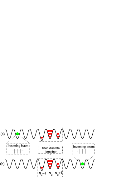
Figure 1: The transport scheme under the consideration. Large green dots denote identical incident wave packets coming from the left in (a) and the right in (b). The middle part schematically shows the TDB, where $\varepsilon_{n}=0$, except for $\varepsilon_{n_{c}-1}<0$.

From Eq. (7), one can obtain different types of stationary solutions. For the symmetric configuration with $\varepsilon_{1}=\varepsilon_{3}$, the stationary states correspond to ordinary symmetric DBs, which have been investigated in detail, including their formation RLivi2006 ; GSNg2009 and transport properties RFranzosi2007 ; XDBai2012 ; HHennig2010 . On the other hand, the setting with $\varepsilon_{1}\neq\varepsilon_{3}$ gives rise to TDB, as schematically shown in the middle part of Fig. 1, where $n_{c}-1$, $n_{c}$, and $n_{c}+1$ may be regarded as $1$, $2$, and $3$, respectively, in the trimer model.

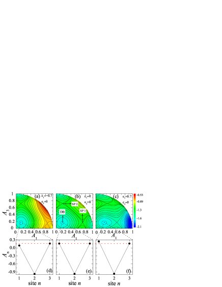
Figure 2: (a)-(c) Contour plots of energy given by Eq. (8) for different $\varepsilon_{1}$ with fixed $\lambda=3$ and $\varepsilon_{3}=0$. (d)-(f) The structure of the DB corresponding to panels (a)-(c), respectively. SP1 and SP2 denote the saddle points.

Here, our aim is to investigate the transport of lattice waves through the TDB, for the wave packets arriving from the opposite directions (see Fig. 1). To this end, we consider the system’s Hamiltonian for configurations taken in the form of Eqs. (4) and (5), which must be taken with the opposite overall sign, due to the above-mentioned staggering transformation:

$$H=-\frac{\lambda}{2}\!\left(A_{1}^{4}\!+\!A_{2}^{4}\!+\!A_{3}^{4}\right)\!-\!\left(\varepsilon_{1}A_{1}^{2}\!+\!\varepsilon_{3}A_{3}^{2}\right)\!-\!\left(A_{1}\!+\!A_{3}\right)\!A_{2}.$$ (8)

The effect of $\varepsilon_{n}$ on the Hamiltonian, considered as a function of $A_{1}$ and $A_{3}$, is shown in Figs. 2(a)-2(c), which exhibits three minima separated by two saddle points SP1 and SP2. The minima refer to the DBs, whose structure is displayed in Figs. 2(d)-2(f) (the trimer model per se was studied in detail in Ref. GKopidakis2000 ). Analytical solutions for SP1, SP2, and DB can be obtained from Eq. (7) in the limit of large $\lambda$ and $\varepsilon_{1},\varepsilon_{3}\rightarrow 0$. Similar to the results of Ref. GKopidakis2000 , the respective energies of SP1 and SP2, $E_{\mathrm{thr}1,2}$, which play the role of thresholds for the perturbed dynamics of the trimer (see below), are

$$E_{\mathrm{thr}1}\! = \!-\!\frac{1}{2}-\frac{\lambda}{4}-\frac{1}{4\lambda}+\frac{1}{4\lambda^{2}}-\frac{1}{4\lambda^{3}}+\frac{9}{16\lambda^{4}}$$ (9)

$$-\varepsilon_{1}\!\!\left(\!\frac{1}{2}\!+\!\!\frac{1}{2\lambda^{3}}\!-\!\frac{5}{8\lambda^{4}}\!\right)\!\!+\!\varepsilon_{1}^{2}\!\!\left(\!\!\frac{1}{4\lambda}\!+\!\!\frac{1}{4\lambda^{2}}\!+\!\!\frac{1}{16\lambda^{3}}\!+\!\!\frac{3}{16\lambda^{4}}\!\!\right)$$

$$-\varepsilon_{1}^{3}\left(\frac{1}{8\lambda^{3}}+\frac{1}{16\lambda^{4}}\right)\!\!-\!\varepsilon_{3}\!\!\left(\!\!\frac{1}{2\lambda^{2}}\!-\!\frac{1}{\lambda^{3}}\!+\!\frac{1}{2\lambda^{4}}\!\!\right)\!,$$

$$E_{\mathrm{thr}2}\! = \!-\!\frac{1}{2}-\frac{\lambda}{4}-\frac{1}{4\lambda}+\frac{1}{4\lambda^{2}}-\frac{1}{4\lambda^{3}}+\frac{9}{16\lambda^{4}}$$ (10)

$$-\varepsilon_{3}\!\!\left(\!\frac{1}{2}\!+\!\!\frac{1}{2\lambda^{3}}\!-\!\frac{5}{8\lambda^{4}}\!\right)\!\!+\!\varepsilon_{3}^{2}\!\!\left(\!\!\frac{1}{4\lambda}\!+\!\!\frac{1}{4\lambda^{2}}\!+\!\!\frac{1}{16\lambda^{3}}\!+\!\!\frac{3}{16\lambda^{4}}\!\!\right)$$

$$-\varepsilon_{3}^{3}\left(\frac{1}{8\lambda^{3}}+\frac{1}{16\lambda^{4}}\right)\!\!-\!\varepsilon_{1}\!\!\left(\!\!\frac{1}{2\lambda^{2}}\!-\!\frac{1}{\lambda^{3}}\!+\!\frac{1}{2\lambda^{4}}\!\!\right)\!.$$

In the case of $\varepsilon_{1}=\varepsilon_{3}=0$, which corresponds to Fig. 2(b), the discrete solitons corresponding to SP1, SP2, and the DB are symmetric, as shown in Fig. 2(e). On the other hand, the asymmetric setting, with

$$\varepsilon_{1}<0,\;\;\;\;\;~{}\varepsilon_{2}=\varepsilon_{3}=0,$$ (11)

with $\varepsilon_{1}=-0.7$, is represented by Fig. 2(a). In this case, the discrete soliton becomes a TDB, as shown in Fig. 2(d), where the norm (alias power, in terms of optics) localized at site $1$ is smaller than in the symmetric case. SP2 remains nearly the same as in the symmetric case, while SP1 moves away from the TDB. The relationship between energy thresholds in this case is $E_{\mathrm{thr}1}>E_{\mathrm{thr}2}$. Similarly, we set $\varepsilon_{3}=0$ and $\varepsilon_{1}=0.7>0$ in Fig. 2(c), which again gives rise to a TDB, with the norm (power) at site $1$ larger than that in the symmetric case, see Fig. 2(f). In this case, SP2 remains nearly unaffected, while SP1 moves towards the TDB, and the relationship between the energy thresholds is $E_{\mathrm{thr}1}<E_{\mathrm{thr}2}$. Note that, in the limit of $\varepsilon_{1}\rightarrow-\infty$, SP1 will disappear and value $E_{\mathrm{thr}1}$ cannot be reached, as shown in Fig. 8(a) in the Appendix.

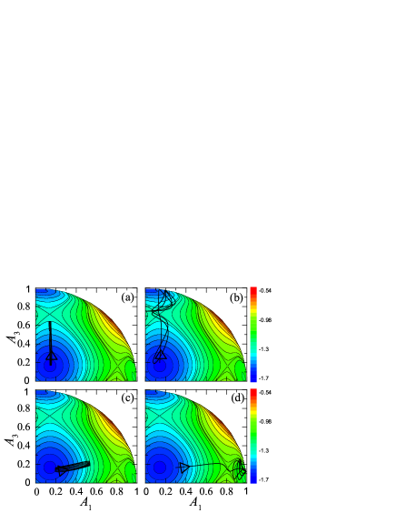
Figure 3: Dynamics of the trimer initiated by the perturbations applied at site $3$ [(a),(b)] or at site $1$ [(c),(d)]. Here $E_{\mathrm{thr}1}=-1.01787>E_{\mathrm{thr}2}=-1.29859$ correspond to SP1 and SP2, respectively. (a) $H=-1.319<E_{\mathrm{thr}2}$, and the orbit cannot climb over SP2. (b),(c) $E_{\mathrm{thr}2}<H=-1.263<E_{\mathrm{thr}1}$, hence the orbit can pass SP2, but cannot pass SP1. (d) $H=-1.011>E_{\mathrm{thr}1}$, and the orbit can climb over the SP1. Perturbation parameters in Eq. (12) are $\delta A_{3}=0.004528$ in (a) and $\delta A_{3}=0.032866$ in (b). Similarly, perturbations applied at site $1$ are $\delta A_{1}=0.055125$ in (c) and $\delta A_{1}=0.158584$ in (d). In all the cases, $\lambda=3$, $\varepsilon_{1}=-0.5$, $\varepsilon_{3}=0$, $A_{1}^{\mathrm{TDB}}=0.1412,A_{3}^{\mathrm{TDB}}=0.1664$, and $\delta\theta=\pi$.

III Unidirectional transport of wave packets

To study the transport of matter waves through the TDB in opposite directions, we first consider the incident wave coming from the right. In terms of the natural representation, $\psi_{n}(t)=A_{n}e^{i\theta_{n}}$, where $A_{n}$ and $\theta_{n}$ are amplitudes and phases at site $n$, the corresponding initial conditions for the trimer approximation may be considered as the stationary TDB disturbed at site $3$:

$$\psi{(t=0)}=\left\{A_{1}^{\mathrm{TDB}},A_{2},(A_{3}^{\mathrm{TDB}}+\delta A_{3})e^{i\delta\theta}\right\},$$ (12)

with $A_{2}=-\sqrt{1-|\psi_{1}|^{2}-|\psi_{3}|^{2}}$, perturbation amplitude $\delta A_{3}$ added at site $3$, and the corresponding phase $\delta\theta$. The resulting evolution of the trimer system, initiated by the perturbation, is shown by black trajectories in Fig. 3 for fixed $\lambda=3$, $\varepsilon_{1}=-0.5$, and $\varepsilon_{3}=0$, so that $E_{\mathrm{thr}1}=-1.01787>E_{\mathrm{thr}2}=-1.29859$. If the perturbation is small, the total energy of the system, $H$, remains smaller than $E_{\mathrm{thr}2}$, hence the orbit is not able to climb over saddle point SP2, while the TDB remains stable. That is, for this case nothing is transferred to site $1$, as shown in Fig. 3(a). If the perturbation is large, so that $H>E_{\mathrm{thr}2}$, the orbit can pass saddle point SP2, and a part of the norm (power) is transferred to site $1$, as shown in Fig. 3(b).

If the incident wave comes from the left, it can be considered as the perturbation added to the stationary TDB at site $1$. Then, one arrives at similar conclusions. First, if the perturbation is small, no transport takes place, as shown in Fig. 3(c). Next, if the perturbation is large, leading to $H>E_{\mathrm{thr}1}$, a part of the norm (power) is transferred to site $3$, as shown in Fig. 3(d).

Note that in Figs. 3(b) and 3(c) we have chosen identical initial conditions, i.e., there are the same energies of the TDB, $H$, and the same incident excitations, coming from the opposite directions. Thus, it follows from the above considerations that, in the intermediate case,

$$E_{\mathrm{thr}2}<H<E_{\mathrm{thr}1},$$ (13)

the transport from one side to the other can take place in Fig. 3(b), while it is forbidden in Fig. 3(c). In other words, the same incident wave can pass from right to left, but not in the opposite direction, which implies non-reciprocal transmission.

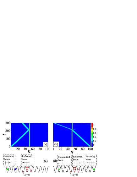
Figure 4: The transfer of incident waves through the stationary TDB in the long lattice ($M=101$ sites), for identical excitations arriving from the left in (a) and from the right in (b), respectively. Colors represent norms at the sites. In (c) and (d), the small and red circles depict the TDBs located, essentially, at sites $50,51$, and $52$, with $A_{50}=0.1502$, $A_{51}=0.974553$, $A_{52}=0.166384$. Circles of different size and color represent the incident, reflected, and transmitted excitations. The amplitudes of the incident excitations are $A_{1}=A_{4}=0.2$ and $A_{2}=A_{3}=0.4$, and its energy is $\delta E=0.39743$. The energy thresholds are $E_{\mathrm{thr}1}=-1.14325$ in (a) and $E_{\mathrm{thr}2}=-1.30276$ in (b) for the excitations arriving from the left and right, respectively. In all the cases, $\lambda=3$, $\varepsilon_{n}=0$, except for $\varepsilon_{50}=-0.3$, and $E_{\mathrm{TDB}}=-1.6573$.

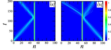
Figure 5: The transfer of incident waves through the stationary TDB in the long lattice ($M=101$ sites) with weaker intrinsic nonlinearity of identical excitations arriving from the left in (a) and the right in (b), respectively (cf. Fig. 4 where the effective nonlinearity of the incident pulses is stronger by a factor $\approx 3$). The TDB is located, essentially, at sites $50,51$, and $52$. The amplitudes of the incident excitations are $A_{1}=A_{4}=0.16$ and $A_{2}=A_{3}=0.32$. In all the cases, $\lambda=2.5$, $\varepsilon_{n}=0$, except for $\varepsilon_{50}=-0.8$, $\varepsilon_{52}=0.5$.

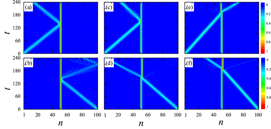
Figure 6: The transfer of incident waves through the stationary TDB in the long lattice ($M=101$ sites) with different energies. Colors represent norms at the sites. The amplitudes of the incident excitations are $A_{2}=A_{3}=0.32$, and its energy is $\delta E=0.2594<0.271$ in (a) and (b); $A_{2}=A_{3}=0.35$ and $0.271<\delta E=0.2966<0.315$ in (c) and (d); $A_{2}=A_{3}=0.4$ and $\delta E=0.38395>0.315$ in (e) and (f). In all the cases, $A_{1}=A_{4}=0.18$, $\lambda=3$, $\varepsilon_{n}=0$, except for $\varepsilon_{50}=-0.05$.

Next, we have performed systematic simulations of the transport of the incident waves in the full extended lattice of size $M=101$ with the embedded TDB. The first typical example is displayed in Fig. 4, where the incident waves arrive from the left or right to collide with the TDB, as shown in Figs. 4(c) and 4(d), respectively. Initially, the TDB is taken in the stationary form predicted by the trimer model, the respective energy thresholds being $E_{\mathrm{thr}1}=-1.14325$ and $E_{\mathrm{thr}2}=-1.30276$, with $\lambda=3$, $\varepsilon_{1}=-0.3$, $\varepsilon_{3}=0$, and $H_{\mathrm{TDB}}=-1.6573$. The initial condition for the incident wave packet was set on four sites of the lattice, $\psi_{\mathrm{in}}(t)=\{A_{n}e^{i\theta_{n}},~{}n=1,2,3,4\},$ with phase shifts corresponding to the staggered ansatz, $\delta\theta_{12}=\delta\theta_{23}=\delta\theta_{34}=\pi$, where $\delta\theta_{jk}=\theta_{j}-\theta_{k}$, cf. Eq. (5). Its energy $\delta E=\sum_{n=1}^{4}\frac{\lambda}{2}A_{n}^{4}+\sum_{n=1}^{3}A_{n}A_{n+1}\cos\theta_{n,n+1}=0.39743$, hence the total energy, including the TDB and the incident wave, is

$$E_{t}=H_{\mathrm{TDB}}+\delta E.$$ (14)

The most interesting case for the simulations is

$$E_{\mathrm{thr}2}<E_{t}<E_{\mathrm{thr}1},$$ (15)

as Eq. (13) suggests that the unidirectional transfer may be expected in this case [parameters of Fig. 4 comply with Eq. (15)]. The simulations confirm this expectation: while the wave arriving from the left is entirely reflected by the TDB, as seen in Figs. 4(a) and 4(c), the one coming from the right is chiefly transmitted through the TDB, although a weak component is reflected, as seen in Figs. 4(b) and 4(d).

Note that, as seen in Fig. 4(b), the impact of the incident packet which passes the TDB leads to a shift of the TDB by one site in the direction from which the packet has arrived. The shift actually takes place against the lattice-potential slope, as seen from Eq. (11). The shift, which is explained by the mutual nonlinear attraction between the incident and pinned modes, is, as a matter of fact, a manifestation of the tractor-beam effect, that has recently drawn much interest in optics tractor . On the other hand, Fig. 4(a) shows that the reflected wave packet does not shift the pinned TDB, which is explained by the balance of the attraction and recoil effects.

If the lattice contains only isolated defects embedded into a regular host medium, the shifts produced by single or multiple scatterings of wave packets may draw the TDB into a uniform section, where the diode effect will disappear. On the other hand, if the lattice is built as a chain of defects of type (11), i.e., weak asymmetry is present at each site, the diode and tractor-beam effects may possibly persist in multiple collisions of incident wave packets with the TDB, until the gradually drifting TDB will hit the edge of the system (the left edge, if the wave packets arrive from the left). Of course, the mean potential slope in such a tilted lattice will eventually give rise to reflection of any incident wave packet, in the absence of the TDB; however, the respective reflection length is much larger than that induced by the TDB, hence the diode effect may plausibly remain discernible in the tilted lattice.

In Fig. 4, the examples of the transmission and reflection are demonstrated for incident wave packets which carry relatively strong nonlinearity. Similar results for incident wave packets with the strength of the intrinsic nonlinearity weaker by a factor of $3$ than in Fig. 4 are displayed in Fig. 5. It is seen that the diode effect acts in this case too. On the other hand, the effect cannot take place for linear wave packets (ones with a very small amplitude), as, having small energies, they do not satisfy condition (15).

Another set of characteristic examples is plotted in Fig. 6, where, keeping fixed parameters of the defect and TDB pinned to it, we illustrate the change of the scattering scenario with the increase of energy $\delta E$ of the incident wave packet. As predicted by the above analysis, at small energies, corresponding to $E_{t}<E_{\mathrm{thr}2}$, see Eq. (14), Figs. 6(a) and 6(b) corroborate that the wave packets cannot pass the TDB in either direction. On the other hand, the diode and tractor-beam effects act in Figs. 6(c) and 6(d), which was generated for $\delta E$ complying with Eq. (15). Lastly, Figs. 6(e) and 6(f), which corresponds to $E_{t}>E_{\mathrm{thr}1}$, demonstrates that left- and right-arriving wave packets easily pass the TDB. In the latter case, the “tractor-beam” effect takes place for either incidence direction.

Collecting results of the simulations for the full lattice, we conclude that $\delta E$ may be used as an efficient control parameter to govern the outcome of the collision of the incident wave packet with the given TDB, in accordance with Eq. (15). To clearly display the results, in Fig. 7 we present the reflection, transmission, and absorption coefficients, defined in terms of the energy, for the passage of the left- and right-incident wave packets through the given TDB versus $\delta E$ in the long lattice ($M=101$ sites), “absorption” meaning that a part of the energy of the incident wave may be spent on weak excitation of the quiescent TDB. Here, the initial conditions similar to those in Fig. 6, with the incident excitation having $A_{1}=A_{4}=0.18$, while its energy, $\delta E$, is adjusted by varying the value of $A_{2}=A_{3}$.The sum of the three coefficients is $1$, as it must be. In region I, $E_{t}<E_{\mathrm{thr}2}<E_{\mathrm{thr}1}$, the transmission coefficients for both the left- and right-incident waves are practically zero. In the middle region II, which corresponds to Eq. (15), only the right-incident wave passes the TDB, while the left wave is reflected, i.e., the TDB-induced diode effect takes place. The effect can be controlled by adjusting $\varepsilon_{n-1}$ and $\varepsilon_{n+1}$. Finally, in region III, $E_{\mathrm{thr}2}<E_{\mathrm{thr}1}<E_{t}$, the TDB is passable in both directions. In particular, if $\varepsilon_{n-1}\rightarrow-\infty$, SP1 disappears [see Fig. 8(a) in the Appendix], and region III does not exist. In the latter case, the incident wave packets cannot pass the TDB from left to right, irrespective of $\delta E$, and the TDB tends to acts as a “full diode”.

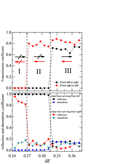
Figure 7: The transmission, reflection, and absorption coefficients for the passage through the stationary TDB in the long lattice ($M=101$ sites) of the same incident wave packet arriving from the left and from the right, as functions of its energy, $\delta E$. The energy thresholds for the excitation coming from the left and right satisfy $E_{\mathrm{thr}1}>E_{\mathrm{thr}2}$, and $\rightarrow$ ($\nrightarrow$) implies that the incident wave can (cannot) pass the TDB. Regions I, II, and III are defined by, respectively, $E_{t}<E_{\mathrm{thr}2}$, $E_{\mathrm{thr}2}<E_{t}<E_{\mathrm{thr}1}$, and $E_{t}>E_{\mathrm{thr}1}$. The TDB is located, essentially, at sites $50,51$, and $52$, with $A_{50}=0.163359$, $A_{51}=0.972447$, and $A_{52}=0.166316$. In all the cases, $\lambda=3$ and $\varepsilon_{n}=0$, except for $\varepsilon_{50}=-0.05$.

IV Conclusion

We have investigated the transport of waves through the TDB in the framework of the DNLS model with the asymmetric on-site defect potential. As a result, the diodelike transport mode has been found, i.e., the unidirectional transfer of the waves across the TDB, in a finite interval of energies of the incident wave packet, while the underlying lattice itself (without the TDB placed at a desired position) cannot operate in such a regime. The underlying mechanism is accurately explained by the consideration of respective energy barriers. If the incident wave packet passes the pinned TDB, the “tractor-beam” effect takes place, with the TDB shifting by one lattice site in the incidence direction, due to its attraction to the incident pulse. The bouncing wave packet does not cause the shift, the attraction being balanced by the recoil.

In the experimental realization of the system in BEC, the defect potential can be created, respectively, as a barrier or well, by a blue- or red-detuned laser beam illuminating the BEC at a particular site ATrombettoni2002 ; JELye2005 ; CFort2005 . In terms of optical waveguide arrays, the potential can be induced by altering the effective refractive index in particular cores. The results suggest a scheme for the implementation of controlled blocking, filtering, and routing of matter-wave and optical beams in guiding networks, as well as for the realization of the tractor-beam mechanism. In particular, the scheme may be useful for steering matter waves in interferometry and quantum-information processing RAVicencio2007 . In addition to working with the atom and optical beams, the present results may find applications in various other contexts to which the DNLS model applies.

Appendix: The consideration of limit cases

In the main text, we mainly consider the passage of wave packets in the opposite directions through the TDB  pinned by the asymmetric local potential. As a result, we have found that the unidirectional passage (the diode effect) strongly depends on the total energy, $E_{t}$, and the threshold energies, $E_{\mathrm{thr}1,2}$. As shown in Fig. 7 in the main text, the TDB is impassable for the wave packets arriving from either side in the case of $E_{t}<E_{\mathrm{thr}2}<E_{\mathrm{thr}1}$, which is defined as region I, and passable in region III, $E_{\mathrm{thr}2}<E_{\mathrm{thr}1}<E_{t}$. On the other hand, in region II, which corresponds to $E_{\mathrm{thr}2}<E_{t}<E_{\mathrm{thr}1}$, the incident wave passes the TDB unidirectionally (from right to left in Fig. 4 of the main text), with a high transmission coefficient. Here, we discuss limit cases in which the absolute value of $\varepsilon_{1}$ is large enough.

In the main text it has been demonstrated that the left- (right-) incident wave packet passes the TDB only when its energy exceeds $E_{\mathrm{thr}1}$ ($E_{\mathrm{thr}2}$). That is, the TDB creates different potential barriers $E_{\mathrm{thr}1}$ and $E_{\mathrm{thr}2}$ for the same wave packet arriving from the different directions. The effect of coefficients $\varepsilon_{n}$, that determine the local defect, on the Hamiltonian, considered as a function of $A_{1}$ and $A_{3}$, is shown in Figs. 2(a) and 2(c) in the main text. When $\varepsilon_{3}=0$ and $\varepsilon_{1}=-0.7$, the discrete soliton is a TDB, with $E_{\mathrm{thr}1}>E_{\mathrm{thr}2}$. In this case, although it is harder for the wave packet to pass the TDB from left to right, it still can do that at $E_{t}>E_{\mathrm{thr}1}$. However, when $\varepsilon_{1}$ is negative, and its absolute is large, the energy at saddle point SP1 is much higher than at SP2, i.e., $E_{\mathrm{thr}1}\gg E_{\mathrm{thr}2}$, as shown in Fig. 8(b). In particular, when $|\varepsilon_{1}|$ is large enough, SP1 disappears, and value $E_{\mathrm{thr}1}$ cannot be reached, as shown in Fig. 8(a) (cf. the consideration of the trimer system in Ref. GKopidakis2000 ). Effectively, in the latter case, the TDB is an infinitely high potential barrier for the wave packet arriving from the left. Hence, irrespective of the magnitude of $E_{t}$, the wave packet cannot pass the TDB from left to right. (as long as the norm of the scattering wave is not too large compared to the norm of the scattering TDB). On the other hand, when $\varepsilon_{1}$ is positive and large enough, SP1 and DB disappear. Accordingly, thresholds $E_{\mathrm{thr}1,2}$ lose their meaning, as shown in Figs. 8(c) and 8(d). Note that the transfer of the wave packet through the TDB from right to left can be controlled by means of potential parameter $\varepsilon_{3}$.

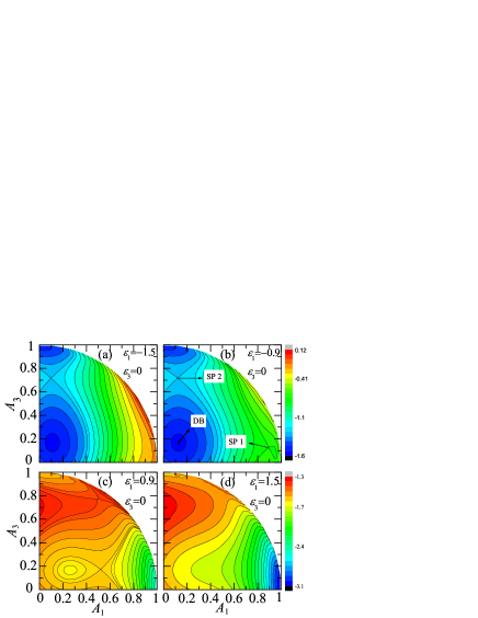
Figure 8: Contour plots of the energy given by Eq. (8) from the main text when the absolute value of $\varepsilon_{1}$ is large enough, with fixed $\lambda=3$ and $\varepsilon_{3}=0$. SP1 and SP2 denote the saddle points.

References

- (1) A. J. Sievers and J. B. Page, in Phonon Physics: The Cutting Edge, Dynamical Properties of Solids Vol. VII (Elsevier, Amsterdam, 1995); S. Aubry, Physica (Amsterdam) 103D, 201 (1997); S. Flach and A. V. Gorbach, Phys. Rep. 467, 1 (2008); J. W. Fleischer, M. Segev, N. K. Efremidis, and D. N. Christodoulides, Nature (London) 422, 147 (2003).
- (2) S. Flach and C. R. Willis, Phys. Rep. 295, 181 (1998).
- (3) P. G. Kevrekidis, The Discrete Nonlinear Schrödinger Equation: Mathematical Analysis, Numerical Computations, and Physical Perspectives (Berlin: Springer, 2009).
- (4) M. Sato, B. E. Hubbard, and A. J. Sievers, Rev. Mod. Phys. 78, 137 (2006).
- (5) E. Trias, J. J. Mazo, and T. P. Orlando, Phys. Rev. Lett. 84, 741 (2000).
- (6) A. V. Ustinov, Chaos 13, 716 (2003).
- (7) D. N. Christodoulides and R. I. Joseph, Opt. Lett. 13, 794 (1988).
- (8) R. Morandotti, U. Peschel, J. S. Aitchison, H. S. Eisenberg, and Y. Silberberg, Phys. Rev. Lett. 83, 2726 (1999).
- (9) F. Lederer, G. I. Stegeman, D. N. Christodoulides, G. Assanto, M. Segev, and Y. Silberberg, Phys. Rep. 463, 1 (2008); Y. V. Kartashov, V. A. Vysloukh, and L. Torner, Progr. Opt. 52, 63 (2009); U. Röpke, H. Bartelt, S. Unger, K. Schuster, and J. Kobelke, Appl. Phys. B 104, 481 (2011).
- (10) F. Eilenberger, S. Minardi, A Szameit, U. Röpke, J. Kobelke, K. Schuster, H. Bartelt, S. Nolte, A. Tünnermann, and T. Pertsch, Opt. Express 19, 23171 (2011).
- (11) U. T. Schwarz, L. Q. English, and A. J. Sievers, Phys. Rev. Lett. 83, 223 (1999).
- (12) M. Sato and A. J. Sievers, Nature (London) 432, 486 (2004).
- (13) A. Trombettoni and A. Smerzi, Phys. Rev. Lett. 86, 2353 (2001); F. K. Abdullaev, B. B. Baizakov, S. A. Darmanyan, V. V. Konotop, and M. Salerno, Phys. Rev. A 64, 043606 (2001); R. Carretero-González and K. Promislow, Phys. Rev. A 66, 033610 (2002); G. I. Alfimov, P. G. Kevrekidis, V. V. Konotop, and M. Salerno, Phys. Rev. E 66, 046608 (2002).
- (14) B. Eiermann, T. Anker, M. Albiez, M. Taglieber, P. Treutlein, K. P. Marzlin, and M. K. Oberthaler, Phys. Rev. Lett. 92, 230401 (2004); O. Morsch and M. Oberthaler, Rev. Mod. Phys. 78, 179 (2006).
- (15) V. A. Brazhnyi and V. V. Konotop, Mod. Phys. Lett. B 18, 627 (2004).
- (16) E. B. Kolomeisky and J. P. Straley, Phys. Rev. B 46, 11749 (1992); E. B. Kolomeisky, T. J. Newman, J. P. Straley, and X. Qi, Phys. Rev. Lett. 85, 1146 (2000).
- (17) J. K. Xue and A. X. Zhang, Phys. Rev. Lett. 101, 180401(2008); A. X. Zhang and J. K. Xue, Phys. Rev. A 80, 043617 (2009).
- (18) M. G. Clerc, R. G. Elias, and R. G. Rojas, Phil. Trans. R. Soc. London Ser. B 369, 412 (2011).
- (19) P. C. Matthews and H. Susanto, Phys. Rev. E 84, 066207 (2011).
- (20) J. D. Andersen and V. M. Kenkre, Phys. Rev. B 47, 11134 (1993).
- (21) M. Peyrard, T. Dauxois, H. Hoyet, and C. R. Willis, Physica D 68, 104 (1993).
- (22) R. S. MacKay and J. A. Sepulchre, Physica D 119, 148 (1998).
- (23) P. J. Martinez, M. Meister, L. M. Floria, and F. Falo, Chaos 13, 610 (2003).
- (24) G. P. Tsironis and S. Aubry, Phys. Rev. Lett. 77, 5225 (1996).
- (25) R. Livi, R. Franzosi, and G. L. Oppo, Phys. Rev. Lett. 97, 060401 (2006).
- (26) G. S. Ng, H. Hennig, R. Fleischmann, T. Kottos, and T. Geisel, New J. Phys. 11, 073045 (2009).
- (27) R. Franzosi, R. Livi, and G.-L. Oppo, J. Phys. B 40, 1195 (2007).
- (28) X.-D. Bai and J.-K. Xue, Phys. Rev. E 86, 066605 (2012). X.-D. Bai, A.-X. Zhang, and J.-K. Xue 88, 062916 (2013).
- (29) T. Schumm, S. Hofferberth, L. M. Andersson, S. Wildermuth, S. Groth, I. Bar-Joseph, J. Schmiedmayer, and P. Krüger, Nat. Phys. 1, 57 (2005).
- (30) D. Jaksch, H. J. Briegel, J. I. Cirac, C. W. Gardiner, and P. Zoller, Phys. Rev. Lett. 82, 1975 (1999).
- (31) G. K. Brennen, C. M. Caves, P. S. Jessen, and I. H. Deutsch, Phys. Rev. Lett. 82, 1060 (1999).
- (32) J. K. Pachos and P. L. Knight, Phys. Rev. Lett. 91, 107902 (2003).
- (33) A. Kay, J. K. Pachos, and C. S. Adams, Phys. Rev. A 73, 022310 (2006).
- (34) S. Lepri and G. Casati, Phys. Rev. Lett. 106, 164101 (2011); S. Lepri and B. A. Malomed, Phys. Rev. E 87, 042903 (2013).
- (35) K. Gallo, G. Assanto, K. R. Parameswaran, and M. M. Fejer, Appl. Phys. Lett. 79, 314 (2001).
- (36) M. Kulishov, J. M. Laniel, N. Bélanger, J. Azaña, and D. V. Plant, Opt. Express 13, 3068 (2005); S. Ding and G. P. Wang, Appl. Phys. Lett. 100, 151913 (2012).
- (37) M. W. Feise, I. V. Shadrivov, and Y. S. Kivshar, Phys. Rev. E 71, 037602 (2005).
- (38) J.-H. Wu, M. Artoni, and G. C. La Rocca, Phys. Rev. Lett. 113, 123004 (2014); C. Sayrin, C. Junge, R. Mitsch, B. Albrecht, D. O’Shea, P. Schneeweiss, J. Volz, and A. Rauschenbeutel, Phys. Rev. X 5, 041036 (2015).
- (39) V. Grigoriev and F. Biancalana, Opt. Lett. 36, 2131 (2011).
- (40) M. Scalora, J. P. Dowling, C. M. Bowden, and M. J. Bloemer, J. Appl. Phys. 76, 2023 (1994).
- (41) M. J. Ablowitz, C. W. Curtis, and Y.-P. Ma, Phys. Rev. A 90, 023813 (2014); Z. Li, R.-X. Wu, Y. Poo, Z. F. Lin, and Q. B. Li, J. Optics 16, 125004 (2014).
- (42) S. Feng and Y. Wang, Optical Materials 35, 1455 (2013); Opt. Exp. 21, 220 (2013); A. Cicek and B. Ulug, Appl. Phys. B - Lasers and Opt. 113, 619 (2013); L. H. Wang, X. L. Yang, X. F. Meng, Y. R. Wang, S. X. Chen, Z. Huang, and G. Y. Dong, Jpn. J. Appl. Phys. 52, 122601 (2013); P. Wang, C. Ren, P. Han, and S. Feng, Opt. Mater. 46, 195 (2015).
- (43) V. V. Konotop and V. Kuzmiak, Phys. Rev. B 66, 14 (2002).
- (44) F. Biancalana, J. Appl. Phys. 104, 093113 (2008).
- (45) H. Ramezani, T. Kottos, R. El-Ganainy, and D. N. Christodoulides, Phys. Rev. A 82, 043803 (2010); A. Regensburger, C. Bersch, M. A. Miri, G. Onishchukov, D. N. Christodoulides, and U. Peschel, Nature 488, 167 (2012); M.-A. Miri, A. Regensburger, U. Peschel, and D. N. Christodoulides, Phys. Rev. A 86, 023807 (2012); J. D’Ambroise, P. G. Kevrekidis, and S. Lepri, J. Phys. A: Math. Theor. 45, 444012 (2012); J. D’Ambroise, S. Lepri, B. A. Malomed, and P. G. Kevrekidis, Phys. Lett. A 378, 2824 (2014); J. Gear, F. Liu, S. T. Chu, S. Rotter, and J. Li, Phys. Rev. A. 91, 033825 (2015); S. Yu, X. Piao, K. W. Yoo, J. Shin, and N. Park, Opt. Express 23, 24997 (2015); Y. Jia, Y. Yan, S. V. Kesava, E. D. Gomez, and N. C. Giebink, ACS Photonics 2, 319 (2015);
- (46) S. Kirihara, M. W. Takeda, K. Sakoda, and Y. Miyamoto, Solid State Comm. 124, 135 (2002).
- (47) F. Tao, W. Chen, W. Xu, J. T. Pan, and S. D. Du, Phys. Rev. E 83, 056605 (2011).
- (48) P. W. Anderson, Phys. Rev. 109, 1492 (1958).
- (49) J. Billy, V. Josse, Z. Zuo, A. Bernard, B. Hambrecht, P. Lugan, D. Clement, L. Sanchez-Palencia, P. Bouyer, and A. Aspect, Nature (London) 453, 891 (2008).
- (50) G. Kopidakis and S. Aubry, Physica D 130, 155 (1999); G. Kopidakis and S. Aubry, Physica D 139, 247 (2000); G. Kopidakis and S. Aubry, Phys. Rev. Lett. 84, 3236 (2000).
- (51) L. Fallani, J. E. Lye, V. Guarrera, C. Fort, and M. Inguscio, Phys. Rev. Lett. 98, 130404 (2007).
- (52) M. I. Molina, Phys. Rev. B 58, 12547 (1998); A. S. Pikovsky and D. L. Shepelyansky, Phys. Rev. Lett. 100, 094101 (2008); S. Flach, D. O. Krimer, and Ch. Skokos, ibid.. 102, 024101 (2009); Ch. Skokos, D. O. Krimer, S. Komineas, and S. Flach, Phys. Rev. E 79, 056211 (2009); H. Veksler, Y. Krivolapov, and S. Fishman, ibid. 80, 037201 (2009); A. Iomin, ibid. E 81, 017601 (2010); E. Lucioni, B. Deissler, L. Tanzi, G. Roati, M. Zaccanti, M. Modugno, M. Larcher, F. Dalfovo, M. Inguscio, and G. Modugno, Phys. Rev. Lett. 106, 230403 (2011); B. Min, T. Li, M. Rosenkranz, and W. Bao, Phys. Rev. A 86, 053612 (2012).
- (53) M. Johansson, G. Kopidakis, and S. Aubry, Europhys. Lett. 91, 50001 (2010).
- (54) Z.-Y. Sun and S. Fishman, Phys. Rev. E 92, 040903(R) (2015).
- (55) D. Jaksch, C. Bruder, J. I. Cirac, C. W. Gardiner, and P. Zoller, Phys. Rev. Lett. 81, 3108 (1998).
- (56) H. Hennig, J. Dorignac, and D. K. Campbell, Phys. Rev. A 82, 053604 (2010).
- (57) A. Novitsky, C.-W. Qiu, and H. Wang, Phys. Rev. Lett. 107, 203601 (2011); S. Sukhov and A. Dogariu, ibid. 107, 203602 (2011); O. Brzobohaty, V. Karasek, M. Siler, L. Chvatal, T. Cizmar, and P. Zemanek, Nature Phot. 7, 123 (2013); V. Shvedov, A. R. Davoyan, C. Hnatovsky, N. Engheta, and W. Krolikowski, ibid. 8, 846 (2014); H. Chen, S. Liu, J. Zi, and Z. F. Lin, ACS Nano 9, 1926 (2015).
- (58) C. Fort, L. Fallani, V. Guarrera, J. E. Lye, M. Modugno, D. S. Wiersma, and M. Inguscio, Phys. Rev. Lett. 95, 170410 (2005).
- (59) J. E. Lye, L. Fallani, M. Modugno, D. S. Wiersma, C. Fort, and M. Inguscio, Phys. Rev. Lett. 95, 070401 (2005).
- (60) A. Trombettoni, A. Smerzi, and A. R. Bishop, Phys. Rev. Lett. 88, 173902 (2002)
- (61) R. A. Vicencio, J. Brand, and S. Flach, Phys. Rev. Lett. 98, 184102 (2007).