Full statistics of erasure processes:
Isothermal adiabatic theory
and a statistical Landauer principle

Abstract. We study driven finite quantum systems in contact with a thermal reservoir in the regime where the system changes slowly in comparison to the equilibration time. The associated isothermal adiabatic theorem allows us to control the full statistics of energy transfers in quasi-static processes. With this approach, we extend Landauer’s Principle on the energetic cost of erasure processes to the level of the full statistics and elucidate the nature of the fluctuations breaking Landauer’s bound.

1 Introduction

Statistical fluctuations of physical quantities around their mean values are ubiquitous phenomena in microscopic systems driven out of thermal equilibrium. Obtaining the full statistics (i.e., the probability distribution) of physically relevant quantities is essential for a complete understanding of work extraction, heat exchanges, and other processes pertaining to these systems. The dominant theoretical and experimental focus in this respect is on classical [ECM, Cr, GC, Ja] and quantum [Ta, Ku] universal fluctuation relations. In our opinion, a task of equal importance is to derive from first principles and experimentally verify the Full Statistics of energy transfers in paradigmatic non-equilibrium processes.

In this note, we contribute to this task by investigating the Full Statistics of the heat dissipated during an erasure process [DL] in the adiabatic limit. While the expected value of this quantity is bounded below by the celebrated Landauer Principle, we show that its Full Statistics possesses extreme outliers: albeit with a small probability, a large heat current breaking Landauer’s bound might be observed. The signature of this phenomena is a singularity of the cumulant generating function of the dissipated heat. Our findings give an additional theoretical prediction to look for in experiments [SSS, PGA] investigating the Landauer bound. The core tool in deriving our results, which is of theoretical interest on its own, is a Full Statistics adiabatic theorem.

Thermodynamics and Information. Thermodynamics and statistical mechanics are intimately linked with information theory through an intriguing world of infernal creatures, thought experiments and analogies. In this world, Maxwell’s demon is effortlessly decreasing the Boltzmann entropy of an ideal gas [Wib], and the Szilard engine is converting the internal energy of a single heat bath into work [Wia]. Both processes are in apparent violation of the second law of thermodynamics. This fundamental law is, however, restored by considering the Shannon entropy of the information acquired by the beings of this world during these processes.

Landauer’s thesis that information is physical [La] provides a guiding principle for exploring the paradoxes of the aforementioned world. Together with Bennett [Be] they argue that information is stored on physical devices and hence its processing has to obey the laws of physics. A bit, an abstract binary variable with values $0/1$, can be implemented by a charge in a capacitor, or a colloidal particle trapped in a double-well. A two level quantum system, called a qubit, can be physically realized by the two energy levels in a quantum dot or in a trapped atom. Irrespective of the realization, the laws of mechanics and thermodynamics apply to these devices.

Conservation of the phase space, in particular, implies that reversible operations (such as the gate mapping $0\to 1$ and vice versa) can be produced with an arbitrary small energy cost, while any irreversible operation would dissipate a certain minimal amount of heat. A paradigmatic example of the latter, invoked when erasing the memory of Maxwell’s demon [Be], is the erasure process (see Figure 1).

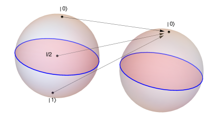
Figure 1: An erasure process maps the Bloch ball, the phase space of a qubit, into a single pure state, e.g., the point $\left|0\right\rangle$. A measurement of the qubit after erasure would not provide any information about the initial state. Since a general quantum operation transforms the Bloch ball into a (possibly degenerate) ellipsoid centered at the image of $I/2$, a process is an erasure process if and only if it maps the completely mixed state $I/2$ into a pure state.

In this process the entire phase space is mapped into a single point. The minimal amount of heat dissipated during this operation is described by the following principle, due to Landauer.

Landauer’s Principle. Specializing to quantum mechanics, we consider the transformation of an initial state $\rho_{\mathrm{i}}$ of a qudit ${\cal S}$ into a final state $\rho_{\rm f}$. If the initial/final entropies $S_{\mathrm{i}/{\rm f}}=-{\rm tr}(\rho_{\mathrm{i}/{\rm f}}\log\rho_{\mathrm{i}/{\rm f}})$ are distinct, then the transition $\rho_{\mathrm{i}}\to\rho_{\rm f}$ is irreversible: it can only be realized by coupling the system ${\cal S}$ to a reservoir ${\cal R}$. The Landauer principle gives a lower bound for the energetic cost of such a transformation in cases when the reservoir is a thermal bath in equilibrium at a given temperature $T=1/k_{B}\beta$. The average heat $\langle\Delta Q\rangle$ dissipated in the reservoir by an arbitrary process which instigates the transition $\rho_{\mathrm{i}}\to\rho_{\rm f}$ is bounded from below as

$$\beta\langle\Delta Q\rangle\geq\Delta S,$$ (1)

where $\Delta S=S_{\mathrm{i}}-S_{\rm f}$ is the entropy difference. If $\rho_{\mathrm{i}}$ is the completely mixed state, and $\rho_{\rm f}$ a pure state, the above process is called erasure. For system with $d$-dimensional Hilbert space, we then have $S_{\mathrm{i}}=\log d$, $S_{\rm f}=0$, and the Landauer bound takes the simple form

$$\beta\langle\Delta Q\rangle\geq\log d.$$ (2)

The Landauer principle is a reformulation of the second law of quantum thermodynamics for qudits [RW, JP]. This can be immediately deduced from the entropy balance equation of the process

$$\Delta S+\langle\sigma\rangle=\beta\langle\Delta Q\rangle.$$ (3)

In one direction, the second law stipulates that the entropy production $\langle\sigma\rangle$ is non-negative, implying Eq. (1), and, in the opposite direction, Inequality (1) implies that $\langle\sigma\rangle\geq 0$. A microscopic derivation of the Landauer Principle was recently given in [RW] for finite dimensional reservoirs and in [JP] for infinitely extended reservoirs. Both works use an appropriate, rigorously justified version of the entropy balance equation (3). Landauer’s Principle was also experimentally confirmed in several classical systems [SLKL, PBVN, Ra, TSU, BAP]; see also the recent reviews [LC, Pe].

Processes involving only finite-volume reservoirs cannot saturate Inequality (1). In fact, tighter lower bounds can be derived in these cases: see [RW] and [GPaM]. In the thermodynamic limit, however, equality is reached by some reversible quasi–static processes [JP]. Such a process is realized by a slowly varying Hamiltonian

$$[0,T]\ni t\mapsto H_{{\cal S}}(t/T)+H_{{\cal R}}+\lambda(t/T)V$$

along any trajectory in the parameter space such that $\lambda(0/1)=0$ and

$$H_{{\cal S}}(0/1)=-\beta^{-1}\log\rho_{\mathrm{i}/{\rm f}}+F_{\mathrm{i}/{\rm f}}I.$$ (4)

Here, $H_{\cal R}$ denotes the Hamiltonian of the reservoir and $V$ its coupling to the system ${\cal S}$, while $F_{\mathrm{i}/{\rm f}}$ are arbitrary constants. In the adiabatic limit $T\to\infty$, the unitary evolution generated by the corresponding Schrödinger equation on the time interval $[0,T]$ transforms the initial state $\rho_{\rm i}$ of the system ${\cal S}$ to its final state $\rho_{\rm f}$, and the equality holds in (1). The quantity $\Delta F=F_{\rm f}-F_{\mathrm{i}}$ is endowed with the meaning of a free energy difference.

Heat Full Statistics. In this work we study the fine balance between heat $\Delta Q$ and entropy $\Delta S$ in such quasi–static transitions, beyond the average value $\langle\Delta Q\rangle$. To saturate Landauer’s bound, we have to work with infinitely extended reservoirs and infinitely slow driving forces, so the definition of $\Delta Q$ is subtle.

The notion of Full Statistics (FS) was introduced in the study of quantum transport [SS, LL1, LL2, LLY] (see also [ABGK, JOPP] for more mathematically oriented approaches) in order to characterize the charge fluctuations in mesoscopic conductors in terms of higher cumulants of their statistical distribution. The later extension of FS to a more general setting, including energy transfers, led to the formulation of fluctuation relations in quantum physics [Ku, Ta]. In this approach, energy variations are not associated to a single observable [TLH] but to a two-time measurement protocol.

Following the works of Kurchan and Tasaki [Ku, Ta] we identify the FS of the dissipated heat $\Delta Q$ with that of the variation in the reservoir energy during the process. This variation is defined as the difference between the outcomes of two energy measurements: one at the initial time $0$ and another one at the final time $T$. The FS of $\Delta Q$ is the probability distribution (pdf) of the resulting classical random variable. The detailed derivation of this FS is given in Section 1.1.

We want to emphasize that the extended reservoir has infinite energy and a continuum of modes. Consequently, to obtain the FS of $\Delta Q$ one has to start with finite reservoirs and perform the thermodynamic limit of the measurement protocol. In this limit, and for generic processes, the random variable $\Delta Q$ acquires a continuous range.

Our main result is an explicit formula for the probability distribution of $\Delta Q$ in the above quasi–static processes which saturate the erasure Landauer bound (2). We show that for the completely mixed initial state $\rho_{\mathrm{i}}=I/d$ and a strictly positive final state $\rho_{\rm f}$ the cumulant generating function of the dissipated heat is given by

$$\log\langle{\rm e}^{-\alpha\Delta Q}\rangle=-\frac{\alpha}{\beta}\log d+\log{\rm tr}\left(\rho_{\rm f}^{1-\frac{\alpha}{\beta}}\right).$$ (5)

Assuming for simplicity that $\rho_{\rm f}$ has the simple spectrum $0<p_{1}<p_{2}<\cdots p_{d}<1$, we can restate our result in terms of pdf: a heat $Q_{k}=\beta^{-1}(\log d+\log p_{k})$ is released during the process with probability $p_{k}$.

We obtained a non-generic atomic probability distribution: $\Delta Q$ is a discrete random variable, with each allowed heat quantum $Q_{k}=\beta^{-1}(\log d+\log p_{k})$ corresponding to an eigenvalue $p_{k}$ of the final state. According to Eq. (4), the associated change of the system energy is

$$E_{\rm f}-E_{\mathrm{i}}=-\beta^{-1}\log p_{k}-\beta^{-1}\log d+\Delta F.$$

Energy conservation then implies that the work done on the total system ${\cal S}+{\cal R}$ during the transition is equal to the change of the free energy $\Delta F$. A posteriori the result is hence interpreted as a fine version of reversibility of the process.

In connection with the erasure process, we further need to consider the limiting case where $\rho_{\rm f}$ becomes a pure state and hence $S_{\rm f}\to 0$. In this limit, the probability distribution of $\Delta Q$ acquires extreme outliers captured by the singularity of the cumulant generating function

$$\lim_{S_{\rm f}\to 0}\log\langle{\rm e}^{-\alpha\Delta Q}\rangle=\begin{cases}-\frac{\alpha}{\beta}\log d&\mbox{if }\alpha<\beta,\\ 0&\mbox{if }\alpha=\beta,\\ \infty&\mbox{if }\alpha>\beta.\end{cases}$$ (6)

The first case corresponds to the cumulant generating function of a deterministic heat dissipation $\Delta Q=\beta^{-1}\Delta S=\beta^{-1}\log d$. In particular, we see that $\beta\langle\Delta Q\rangle=\Delta S$ and all higher cumulants vanish. The discontinuity at $\alpha=\beta$ and the value of the moment generating function at that point is enforced by the fact that $\log\langle{\rm e}^{(\beta-\alpha)\Delta Q}\rangle$ is the cumulant generating function of the heat dissipated in the reservoir by the time reversed evolution. The blow up of the moment generating function for $\alpha>\beta$ is the signature of outliers for $\Delta Q<0$.

We believe that the extreme outliers of the heat probability distribution can be experimentally observed. However, to see these bumps one has to look at the whole moment generating function. Moments themselves have no trace of them. A similar phenomena of hidden long tails in an adiabatic limit has been studied in [CJ].

We proceed with an extended description of our setup. In particular we define the dissipated heat through the Full Statistics of the energy change in the reservoir. We then state the results that allow us to compute the moment generating function in details.

1.1 Abstract setup and outline of the heat FS computation

We consider a finite system ${\cal S}$, with $d$-dimensional Hilbert space, interacting during a time interval $[0,T]$ with a reservoir ${\cal R}$ of finite “size” $L$. The dynamics of the joint system ${\cal S}+{\cal R}$ is governed by the Hamiltonian

$$H^{(L)}(t/T)=H_{\cal S}(t/T)+H_{\cal R}^{(L)}+\lambda(t/T)V.$$ (7)

The reservoir Hamiltonian $H^{(L)}_{\cal R}$ and the interaction $V$ are time independent while the time dependent coupling strength $\lambda(t/T)$ and system Hamiltonian $H_{\cal S}(t/T)$ allow us to control the resulting time evolution. In terms of the rescaled time $s=t/T$, called epoch, the propagator $U^{(T,L)}_{s}$ associated to (7) satisfies the Schrödinger equation

$$\frac{1}{T}\mathrm{i}\partial_{s}U^{(T,L)}_{s}=H^{(L)}(s)U^{(T,L)}_{s},\qquad U^{(T,L)}_{0}=I.$$ (8)

In the following we assume that the controls $\lambda(s)$ and $H_{\cal S}(s)$ together with their first derivatives are continuous functions of $s\in[0,1]$. More importantly, we impose the following boundary conditions:

$$\lambda(0)=\lambda(1)=0,$$ (9)

which ensure that the system decouples from the environment at the initial and the final time, and

$$H_{\cal S}(0)=\beta^{-1}\log d+F_{\mathrm{i}},\qquad H_{\cal S}(1)=-\beta^{-1}\log\rho_{\rm f}+F_{\rm f},$$ (10)

where $F_{\mathrm{i}/{\rm f}}$ are arbitrary constants.

The instantaneous thermal equilibrium state at epoch $s$ and inverse temperature $\beta$ is

$$\eta_{s}^{(L)}=\frac{{\rm e}^{-\beta H^{(L)}(s)}}{{\rm tr}({\rm e}^{-\beta H^{(L)}(s)})},$$

which, taking our boundary conditions into account, reduces to

$$\eta_{\mathrm{i}}^{(L)}=\eta_{0}^{(L)}=\frac{I}{d}\otimes\frac{{\rm e}^{-\beta H_{\cal R}^{(L)}}}{{\rm tr}({\rm e}^{-\beta H_{\cal R}^{(L)}})},\qquad\eta_{\rm f}^{(L)}=\eta_{1}^{(L)}=\rho_{\rm f}\otimes\frac{{\rm e}^{-\beta H_{\cal R}^{(L)}}}{{\rm tr}({\rm e}^{-\beta H_{\cal R}^{(L)}})},$$

at the initial/final epoch $s=0/1$. The initial state of the joint system is $\eta_{\mathrm{i}}^{(L)}$, so that its state at epoch $s$ is given by

$$\rho_{s}^{(T,L)}=U^{(T,L)}_{s}\eta_{\mathrm{i}}^{(L)}U^{(T,L)\ast}_{s}.$$

“Local observables” of the joint system ${\cal S}+{\cal R}$ are operators on ${\cal H}^{(L)}$ which, for large enough $L$, do not depend on $L$. We define the thermodynamic limit of the instantaneous equilibrium states on local observables by

$$\eta^{(\infty)}_{s}(A)=\lim_{L\to\infty}{\rm tr}(\eta_{s}^{(L)}A),$$

provided the limit on the right hand side exists.

For large $T$, the system’s drive is slow: during the long time interval $[0,T]$, the variation of the Hamiltonian $H^{(L)}(t/T)$ stays of order $T^{0}$. The adiabatic evolution is obtained by taking the limit $T\to\infty$. The adiabatic theorem for isothermal processes [ASF1, ASF2, JP] states that for any $s\in[0,1]$ and any local observable $A$,

$$\lim_{T\to\infty}\lim_{L\to\infty}{\rm tr}(\rho^{(T,L)}_{s}A)=\eta^{(\infty)}_{s}(A).$$ (11)

We will discuss this relation in more details and give precise conditions for its validity in Section 2.3. Here we just note that the order of limits is important: one first takes the thermodynamic limit $L\to\infty$ and then the adiabatic limit $T\to\infty$.

We identify the dissipated heat $\Delta Q$ with the change of energy in the reservoir as follows. Let $P_{e}^{(L)}$ denote the orthogonal projection on the eigenspace associated to the eigenvalue $e$ of $H^{(L)}_{\cal R}$. The measurement of $H^{(L)}_{\cal R}$ at the initial epoch $s=0$ gives $e$ with a probability ${\rm tr}(P_{e}^{(L)}\eta_{\mathrm{i}}^{(L)})$. After this measurement the system is in the projected state

$$\frac{P_{e}^{(L)}\eta_{\mathrm{i}}^{(L)}P_{e}^{(L)}}{{\rm tr}\left(P_{e}^{(L)}\eta_{\mathrm{i}}^{(L)}\right)}.$$

The second measurement of $H_{\cal R}^{(L)}$ at the final epoch $s=1$, after the system undergoes the transformation described by the propagator $U^{(T,L)}_{1}$, gives $e^{\prime}$ with the probability

$$\frac{{\rm tr}\left(P_{e^{\prime}}^{(L)}U^{(T,L)}_{1}P_{e}^{(L)}\eta_{\mathrm{i}}^{(L)}P_{e}^{(L)}U^{(T,L)\ast}_{1}\right)}{{\rm tr}\left(P_{e}^{(L)}\eta_{\mathrm{i}}^{(L)}\right)}.$$

It follows that, in this measurement protocol, the probability of observing an amount of heat $\Delta Q$ dissipated in the reservoir is

$${\mathbb{P}}^{(T,L)}(\Delta Q)=\sum_{e^{\prime}-e=\Delta Q}{\rm tr}\left(P_{e^{\prime}}^{(L)}U^{(T,L)}_{1}P_{e}^{(L)}\eta_{\mathrm{i}}^{(L)}P_{e}^{(L)}U^{(T,L)\ast}_{1}\right).$$

This distribution is the Full Statistics of the heat dissipation. Its cumulant generating function is

$$\chi^{(T,L)}(\alpha)=\log\sum_{\Delta Q}\mathbb{P}^{(T,L)}(\Delta Q){\rm e}^{-\alpha\Delta Q}=\log{\rm tr}\left({\rm e}^{-\alpha H_{\cal R}^{(L)}}U^{(T,L)}_{1}{\rm e}^{\alpha H_{\cal R}^{(L)}}\eta_{\mathrm{i}}^{(L)}U^{(T,L)\ast}_{1}\right).$$

In view of the boundary conditions (9) and (10) at the epoch $s=0$, the reservoir Hamiltonian $H_{\cal R}^{(L)}$ and the full initial Hamiltonian $H^{(L)}(0)$ differ by a constant. Thus, we can replace the former by the latter in the above relation. Since the relative Rényi $\alpha$-entropy of two states $\rho$, $\sigma$ is defined by

$$S_{\alpha}(\rho|\sigma)=\log{\rm tr}(\rho^{\alpha}\sigma^{1-\alpha}),$$

a simple calculation leads to the identification

$$\chi^{(T,L)}(\alpha)=S_{\frac{\alpha}{\beta}}(\eta_{\mathrm{i}}^{(L)}|\rho^{(T,L)}_{1}).$$ (12)

The existence of the thermodynamic limit of Renyi’s entropy [JOPP] implies that of the FS. Using the adiabatic limit (11) we obtain

$$\lim_{T\to\infty}\lim_{L\to\infty}\chi^{(T,L)}(\alpha)=S_{\frac{\alpha}{\beta}}(\eta^{(\infty)}_{\mathrm{i}}|\eta^{(\infty)}_{\rm f})=S_{\frac{\alpha}{\beta}}(\rho_{\mathrm{i}}|\rho_{\rm f}).$$

The second equality follows from the boundary condition (9): the states $\eta_{\mathrm{i}/{\rm f}}^{(\infty)}$ factorize and their relative entropy is the sum of the relative entropies of each factor. Since the initial and the final state of the reservoir are identical, their relative entropy vanishes and we are left with the relative entropy between the initial and final states of the system ${\cal S}$ alone. Substituting $\rho_{\mathrm{i}}=I/d$ we recover Eq. (5).

A condition regarding the stability of thermal equilibrium states is the main assumption required for the validity of Eq. (11) and our analysis in general (see Section 2.3). Although this condition is expected to hold in a wide class of systems, it is notoriously difficult to prove from basic principles. Spin networks, and generic spin-fermion models are among the relevant systems for which the condition has been rigorously established although most often with a large temperature–weak coupling assumption. We specialize our discussion to one of these models, in which the thermal states are known to be stable for a weak enough interaction. It describes a one dimensional fermionic chain with an impurity. We would like to stress that this choice of model is not central to the results presented here. They hold for any model exhibiting the same stability behaviour at equilibrium.

1.2 A fermionic impurity model

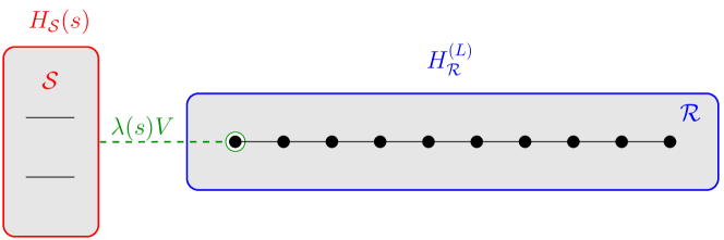
Figure 2: A $2$–level quantum system ${\cal S}$ interacts with a gas of fermions ${\cal R}$ on a one dimensional lattice of size $L$. The epoch-dependent interaction $\lambda(s)V$ couples ${\cal S}$ to the fermions on the first site of this lattice.

We describe a concrete realization of the abstract setup of the previous section. A 2-level quantum system ${\cal S}$ interacts with a reservoir ${\cal R}$, a gas of spinless fermions on a one dimensional lattice of size $L$ (see Figure 2). The system and the reservoir are coupled by a dipolar rotating-wave type interaction between ${\cal S}$ and the fermions on the first site of the lattice. When uncoupled, the reservoir is a free Fermi gas in thermal equilibrium at inverse temperature $\beta$. The thermodynamic limit is obtained by taking the size $L$ of the lattice to infinity. The details are as follows.

The lattice sites are labeled by $x\in\Lambda^{(L)}=\{1,2,\ldots,L\}$. The one-particle Hilbert space of the reservoir is $\ell^{2}(\Lambda^{(L)})$ and we denote by $\delta_{x}$ the delta-function at site $x$. The reservoir is thus described by the antisymmetric Fock space ${\cal H}_{\cal R}^{(L)}=\Gamma(\ell^{2}(\Lambda^{(L)}))$, a $2^{L}$-dimensional Hilbert space. The creation/annihilation operator for a fermion at site $x\in\Lambda^{(L)}$ is $c^{\ast}(x)$/$c(x)$. These operators obey the canonical anti-commutation relation

$$\{c(x),c^{\ast}(x^{\prime})\}=c(x)c^{\ast}(x^{\prime})+c^{\ast}(x^{\prime})c(x)=\delta_{x,x^{\prime}}.$$

The reservoir Hamiltonian

$$H_{\cal R}^{(L)}=\kappa\sum_{\begin{subarray}{c}x,y\in\Lambda^{(L)}\\ |x-y|=1\end{subarray}}c^{\ast}(x)c(y)$$

is the second quantization of $\kappa\Delta^{(L)}$, where $\Delta^{(L)}$ is the discrete Laplacian on $\Lambda^{(L)}$ with Dirichlet boundary conditions,

$$(\Delta^{(L)}f)(x)=\begin{cases}f(2)&\mbox{for }x=1,\\ f(x+1)+f(x-1)&\mbox{for }1<x<L,\\ f(L-1)&\mbox{for }x=L.\\ \end{cases}$$

Thus, $H_{\cal R}^{(L)}$ corresponds to homogeneous hopping between neighboring lattice sites with a hopping constant $\kappa>0$.

The Hilbert space of the system ${\cal S}$ is ${\cal H}_{\cal S}={\mathbb{C}}^{2}$. We denote by $\sigma_{x}$, $\sigma_{y}$ and $\sigma_{z}$ the usual Pauli matrices on ${\cal H}_{\cal S}$. In view of the initial condition $\rho_{\mathrm{i}}=I/2$ and boundary conditions (10), we can assume, without loss of generality, that its Hamiltonian is given by

$$H_{\cal S}(s)=\epsilon(s)I+\gamma(s)\sigma_{z}.$$ (13)

The total Hilbert space is ${\cal H}^{(L)}={\cal H}_{\cal S}\otimes{\cal H}^{(L)}_{\cal R}$. The coupling is achieved by a rotating-wave type interaction between ${\cal S}$ and the fermion on the first lattice site

$$V=\sigma^{-}\otimes c^{*}(1)+\sigma^{+}\otimes c(1),$$

where $\sigma^{\pm}=\frac{1}{2}(\sigma_{x}\pm\mathrm{i}\sigma_{y})$. Note that $V$ is a local observable: it does not depend on the lattice size $L$. This restriction is not strictly necessary but we will not elaborate on this point here.

The Jordan-Wigner transformation maps the fermionic impurity model to a free Fermi gas with one-particle Hilbert space ${\mathbb{C}}\oplus\ell^{2}(\Lambda^{(L)})$ and one-particle Hamiltonian of the Friedrich’s type

$$h(s)=(\epsilon(s)+\gamma(s))I-2\gamma(s)|1\rangle\langle 1|-\lambda(s)(|1\rangle\langle\delta_{1}|+|\delta_{1}\rangle\langle 1|)+\kappa\Delta^{(L)},$$ (14)

where $|1\rangle$ denotes the basis vector of ${\mathbb{C}}$. This allows for a detailed study of the mathematical and physical aspects of this model; see [AJPP1, JKP].

2 Adiabatic limits for thermal states

This section starts with a discussion of the relevant time-scales of the fermionic impurity model of Section 1.2. Then, we investigate the various adiabatic regimes that can be reached by appropriate separations of these time-scales. In particular, we explain why the order of limits in Eq. (11) is relevant for the realization of a quasi-static erasure protocol.

2.1 Time-scales in the impurity model

Adiabatic theory provides a tool to study the dynamics of systems which feature separation of some relevant physical time-scales. To elucidate its meaning in our setup we compare the adiabatic time $T$ with the three relevant dynamical time-scales of our model. We discuss the three adiabatic theorems corresponding to different ordering of $T$ with respect to these time-scales.

For each fixed epoch $s$ we consider the time-scales associated to the dynamics generated by the instantaneous Hamiltonian $H^{(L)}(s)=H_{\cal S}(s)+\lambda(s)V+H_{\cal R}^{(L)}$. In the following discussion we assume that for $s\in]0,1[$ the $s$-dependence of these time-scales is negligible and we omit the variable $s$ from our notation. We reinstate the $s$-dependence in the last paragraph of this subsection.

$T_{\cal S}$: the recurrence time of ${\cal S}$.

This is the quantum analogue of the Poincaré recurrence time, the time after which the isolated ($\lambda=0$) system ${\cal S}$ returns to nearly its initial state; see [BM, CV]. For typical initial states, this time is inversely proportional to the mean level spacing of the system Hamiltonian $H_{\cal S}$. For the fermionic impurity model described in the previous section one has

$$T_{\cal S}\sim\frac{1}{\gamma}.$$

We recall that we use physical units in which energy is the inverse of time, and hence $T_{\cal S}$ is indeed a time-scale.

$T_{{\cal S}+{\cal R}}$: the recurrence time of ${\cal S}+{\cal R}$.

The same as $T_{\cal S}$, but for the coupled ($\lambda\neq 0$) system ${\cal S}+{\cal R}$. The eigenvalues of the discrete Laplacian $\Delta^{(L)}$ are

$$\varepsilon_{k}=2\cos\left(\frac{k\pi}{L+1}\right),\quad(k=1,\ldots,L),$$

and those $H_{\cal R}^{(L)}$ are

$$\kappa\sum_{k=1}^{L}n_{k}\varepsilon_{k},\quad(n_{k}=0,1,2).$$

It follows that the diameter of the spectrum of $H_{\cal R}^{(L)}$ is ${\cal O}(L)$ for large $L$. The same is true for the full Hamiltonian $H^{(L)}$, while $\dim({\cal H}^{(L)})=2^{L+1}$. Thus, the mean level spacing of $H^{(L)}$ is ${\cal O}(L2^{-(L+1)})$ and we conclude that

$$T_{{\cal S}+{\cal R}}=\frac{1}{{\cal O}(L\,2^{-(L+1)})}$$

diverges in the the thermodynamic limit $L\to\infty$.

$T_{m}$: the equilibration time.

This is the time needed for the coupled system ${\cal S}+{\cal R}$ to return to thermal (quasi–)equilibrium after a localized perturbation. In the thermodynamic limit $L=\infty$, the system remains in thermal equilibrium after this time which, in this case, coincides with the mixing time. However, for finite $L$, recurrences appear for times of order $T_{{\cal S}+{\cal R}}$ which is much larger than $T_{m}$. In Section 2.3 we shall argue that for small enough $\lambda>0$, $T_{m}$ stays finite as $L\to\infty$.

In the weak coupling regime, Fermi’s golden rule gives the dependence $T_{m}(\lambda)={\cal O}(\lambda^{-2})$ on the interaction strength $\lambda$. Note in particular that $T_{m}(0)=\infty$. Equilibration is not possible without interaction between ${\cal S}$ and ${\cal R}$.

In the physical systems we have in mind, these time-scales are naturally ordered as

$$T_{\cal S}\ll T_{m}\ll T_{{\cal S}+{\cal R}}.$$

Three physically relevant regimes and one unphysical adiabatic regime are consistent with this ordering (see Figure 3):

1. $T_{\cal S}\ll T\ll T_{m}\ll T_{{\cal S}+{\cal R}}$ (Figure 3 (a)). The adiabatic regime is reached by taking first $L\to\infty$, then $\lambda\to 0$, and finally $T\to\infty$. After the $\lambda\to 0$ limit, the system ${\cal S}$ decouples from the reservoir and the $T\to\infty$ limit yields the standard adiabatic theorem of quantum mechanics [BF, Ka] applied to the isolated system ${\cal S}$.

2. $T_{\cal S}\ll T\sim T_{m}\ll T_{{\cal S}+{\cal R}}$ (Figure 3 (b)). The ordering is the same as in the previous case, but $T$ and $T_{m}$ remain comparable. To reach this regime, one first take $L\to\infty$, and then simultaneously $\lambda\to 0$ and $T\sim\lambda^{-2}\to\infty$. This procedure yields the weak coupling adiabatic theorem of Davies and Spohn [DS, TAS].

3. $T_{\cal S}<T_{m}\ll T\ll T_{{\cal S}+{\cal R}}$ (Figure 3 (c)). This regime corresponds to first taking $L\to\infty$, and then $T\to\infty$ keeping $\lambda\sim{\cal O}(1)$. It is controlled by the adiabatic theorem for isothermal processes [ASF1, ASF2, JP]. After tracing out the degrees of freedom of the reservoir this regime should be equivalent to the Markovian adiabatic theory [SL, Jo, AFGG].

4. $T_{{\cal S}+{\cal R}}\ll T$ (Figure 3 (d)). This unphysical regime is reached by first taking $T\to\infty$. The standard adiabatic theorem applies again, but this time to the joint system ${\cal S}+{\cal R}$. The subsequent thermodynamic limit $L\to\infty$ enforces an infinitely slow driving. We devote the following section to show that the superhero adiabatic theorem associated to this regime gives very different predictions compared to the isothermal adiabatic theorem.

Figure 3: The different time-scale orderings of the adiabatic theorems. In the ordering (a) of the standard adiabatic theorem, the relevant evolution is that of the system ${\cal S}$ with its associated time-scale $T_{\cal S}$. The ordering (c) is associated to the isothermal adiabatic theorem. The ordering for the weak coupling adiabatic theorem (b) is similar with the constraint $T\sim\lambda^{-2}$. In both cases the relevant time-scale is the thermalization time $T_{m}$. The ordering (d) corresponds to the unphysical limit where $T$ is taken to infinity before the thermodynamic limit.

Remark. The family of Hamiltonians $\{H^{(L)}(s)\}_{s\in[0,1]}$ might possess exceptional points at which one or more of the above time-scales diverge. In the standard adiabatic theory these exceptional points correspond to eigenvalue crossings, i.e., accidental degeneracies. The zeroth order adiabatic approximation still holds in the presence of finitely many such exceptional points. In the isothermal adiabatic theory, exceptional points occur whenever $\lambda(s)=0$. Similar to the standard theory, the adiabatic approximation holds also in the presence of finitely many such points. Note in particular that the erasure process has exceptional points at the initial/final epoch $s=0/1$.

2.2 The adiabatic limit for thermal states at finite $L$

Let us apply the standard adiabatic theorem [BF, Ka] to the full Hamiltonian $H^{(L)}(s)$ for finite $L$. For simplicity, we assume that the family $\{H^{(L)}(s)\}_{s\in]0,1[}$ has no exceptional points and admits the representation

$$H^{(L)}(s)=\sum_{k}e_{k}(s)P_{k}(s),$$

where the projections $P_{k}(s)$ are continuously differentiable functions of $s$. Then the adiabatic theorem states that

$$\lim_{T\to\infty}U^{(T,L)}_{s}P_{k}(0)U^{(T,L)\ast}_{s}=P_{k}(s).$$

Hence, given the initial state

$$\eta_{\mathrm{i}}^{(L)}=\frac{{\rm e}^{-\beta H^{(L)}(0)}}{{\rm tr}({\rm e}^{-\beta H^{(L)}(0)})}=\frac{1}{Z_{0}^{(L)}}\sum_{k}{\rm e}^{-\beta e_{k}(0)}P_{k}(0),$$

the final state $\rho^{(T,L)}_{1}$ satisfies

$$\lim_{T\to\infty}\rho^{(T,L)}_{1}=\lim_{T\to\infty}U^{(T,L)}_{1}\eta_{\mathrm{i}}^{(L)}U^{(T,L)\ast}_{1}=\frac{1}{Z_{0}^{(L)}}\sum_{k}{\rm e}^{-\beta e_{k}(0)}P_{k}(1),$$

which only coincides with $\eta_{\rm f}^{(L)}$ if $Z_{0}^{(L)}{\rm e}^{-\beta e_{k}(1)}=Z_{1}^{(L)}{\rm e}^{-\beta e_{k}(0)}$ for all $k$. This is of course a very strong constraint which, in particular, is not satisfied in an erasure protocol.

2.3 The isothermal adiabatic theorem

The main purpose of this section is to formulate a precise statement of the isothermal adiabatic theorem, which is the main technical ingredient of our analysis of quasi-static erasure processes. This requires some preparation and we will start by discussing the thermodynamic limit $L\to\infty$, and in particular the fate of families $\{\rho^{(L)}\}_{L\geq 0}$ of finite volume states in this limit. Then we will introduce the notion of ergodicity which is the main dynamical assumption of the isothermal adiabatic theorem.

The thermodynamic limit.

To avoid technically involved algebraic techniques, we will only work with a potential infinity, i.e., all infinite volume objects will be defined as limits of their finite volume counterparts. A drawback of this approach is that we cannot explain the proof of the isothermal adiabatic theorem, Eq.(11), in details. This proof, which requires the algebraic machinery of quantum statistical mechanics is, however, available in the existing literature [ASF1, ASF2, JP] and it is also given in the companion paper [BFJP]. In the following, we denote all infinite volume quantities with the superscript ^(∞).

A central role in the definition of the thermodynamic limit is played by the set ${\cal A}$ of so-called local observables of the infinite volume system ${\cal S}+{\cal R}$. For our purposes, it will suffice to consider ${\cal A}=\cup_{L\geq 0}{\cal A}^{(L)}$, where ${\cal A}^{(L)}$ is the set of operators which are finite sums of monomials of the form

$$D\otimes c^{\ast}(x_{1})\cdots c^{\ast}(x_{n})c(y_{1})\cdots c(y_{m}),\qquad(x_{i},y_{i}\in\Lambda^{(L)}),$$

where $D$ is an operator on ${\cal H}_{\cal S}$. Note that ${\cal A}^{(L)}\subset{\cal A}^{(L^{\prime})}$ whenever $L\leq L^{\prime}$. By definition, operators in ${\cal A}$ involve only a finite number of lattice sites of the Fermi gas ${\cal R}$ and hence remain well defined as operators on ${\cal H}^{(L)}$ for large enough but finite $L$. In fact, ${\cal A}^{(L)}$ coincides with the set of all operators on ${\cal H}^{(L)}$. In particular, sums and products of elements of ${\cal A}$ are themselves elements of ${\cal A}$ (i.e., ${\cal A}$ is an algebra).

Assume that for each $L\geq 0$, $\rho^{(L)}$ is a density matrix on ${\cal H}^{(L)}$. Given a local observable $A\in{\cal A}$, the expectation $\rho^{(L)}(A)={\rm tr}(\rho^{(L)}A)$ is well defined for large enough $L$. We say that the sequence $\{\rho^{(L)}\}_{L\geq 0}$ has the thermodynamic limit $\rho^{(\infty)}$ whenever, for each $A\in{\cal A}$, the limit

$$\rho^{(\infty)}(A)=\lim_{L\to\infty}{\rm tr}(\rho^{(L)}A)$$

exists. We remark that there may be no density matrix on ${\cal H}^{(\infty)}$ such that $\rho^{(\infty)}(A)={\rm tr}(\rho^{(\infty)}A)$. Nevertheless, the infinite volume state $\rho^{(\infty)}$ defined in this way provides an expectation functional on ${\cal A}$ with the properties $\rho^{(\infty)}(I)=1$ and $0\leq\rho^{(\infty)}(A^{\ast}A)\leq\|A\|^{2}$ for all $A\in{\cal A}$.

We also note that $H_{\cal R}^{(\infty)}$, the energy of the infinite reservoir, is not a local observable and therefore need not have a finite expectation in a thermodynamic limit state $\rho^{(\infty)}$. This is physically consistent with the fact that $\rho^{(\infty)}$ may describe a state of the infinite system with infinite energy (this will indeed be the case for all the thermodynamic limit states relevant to our analysis of erasure processes). On the contrary, $H_{\cal S}$ is a local observable and the energy of the system ${\cal S}$ has finite expectation in any thermodynamic limit state.

Assume now that for each $L\geq 0$, besides the state $\rho^{(L)}$, we also have a unitary propagator $U^{(L)}_{t}$ for the finite system ${\cal S}+{\cal R}$. Since $U^{(L)}_{t}\in{\cal A}^{(L)}$, for any $A\in{\cal A}$ we have $U^{(L)\ast}_{t}AU^{(L)}_{t}\in{\cal A}^{(L)}$ for large enough $L$ so that ${\rm tr}(\rho^{(L)}U^{(L)\ast}_{t}AU^{(L)}_{t})$ is well defined. We shall say that the sequence $\{U^{(L)}_{t}\}_{L\geq 0}$ defines a dynamics for $\rho^{(\infty)}$ on the time interval ${\cal I}$ if

$$\rho^{(\infty)}_{t}(A)=\lim_{L\to\infty}{\rm tr}\left(\rho^{(L)}U^{(L)\ast}_{t}AU^{(L)}_{t}\right)$$

exists for all $A\in{\cal A}$ and all $t\in{\cal I}$. Note that the existence of this limiting dynamics depends not only on the sequence of finite volume propagators, but also on the sequence of finite volume states.

Decades of effort were devoted by the theoretical and mathematical physics communities to the construction and characterization of thermodynamic limit states of quantum systems and their dynamics. We refer the reader to [Ru, BR1, BR2] for detailed expositions of the resulting theory.

Specializing to our impurity model, for each epoch $s$, the instantaneous thermal state $\eta^{(L)}_{s}$ admits a thermodynamic limit $\eta^{(\infty)}_{s}$. Equally importantly for our problem, the propagators $U^{(T,L)}_{s}$ define a dynamics for these states and in particular

$$\rho^{(T,\infty)}_{s}(A)=\lim_{L\to\infty}{\rm tr}\left(\rho^{(T,L)}_{s}A\right)=\lim_{L\to\infty}{\rm tr}\left(\eta_{\mathrm{i}}^{(L)}U^{(T,L)\ast}_{s}AU^{(T,L)}_{s}\right)$$

exists for all $A\in{\cal A}$ and $s\in[0,1]$.

Ergodicity.

As already mentioned in Section 2.1, the adiabatic theory of isothermal processes requires the instantaneous dynamics at each fixed epoch $s$ (with the possible exception of finitely many of them) to have the property that a local perturbations of the instantaneous thermal equilibrium state should relax to this equilibrium state. We now give a more precise statement of this requirement in terms of the ergodic property of the instantaneous dynamics.

Let $\{\rho^{(L)}\}_{L\geq 0}$ be a sequence of finite volume states with thermodynamic limit $\rho^{(\infty)}$. For any non-zero $B\in{\cal A}$, the perturbed states

$$\rho^{(L)}_{B}=\frac{B^{\ast}\rho^{(L)}B}{{\rm tr}(B^{\ast}\rho^{(L)}B)}$$

are well defined for large enough $L$. Using the cyclic property of the trace, one easily shows that

$$\left|{\rm tr}\left(\rho^{(L)}BAB^{\ast}\right)\right|\leq\|A\|{\rm tr}\left(B^{\ast}\rho^{(L)}B\right).$$

Thus, the thermodynamic limit

$$\rho_{B}^{(\infty)}(A)=\lim_{L\to\infty}{\rm tr}\left(\rho_{B}^{(L)}A\right)=\lim_{L\to\infty}\frac{{\rm tr}\left(\rho^{(L)}BAB^{\ast}\right)}{{\rm tr}(\rho^{(L)}BB^{\ast})}=\frac{\rho^{(\infty)}(BAB^{\ast})}{\rho^{(\infty)}(BB^{\ast})}$$

also exists and defines a local perturbation $\rho_{B}^{(\infty)}$ of the state $\rho^{(\infty)}$. Assume that the sequence of Hamiltonians $\{H^{(L)}\}_{L\geq 0}$ defines a dynamics

$$\rho_{B,t}^{(\infty)}(A)=\lim_{L\to\infty}\left(\rho^{(L)}_{B}{\rm e}^{\mathrm{i}tH^{(L)}}A{\rm e}^{-\mathrm{i}tH^{(L)}}\right)$$

on these states. The state $\rho^{(\infty)}$ is said to be ergodic with respect to this dynamics if, for all $A,B\in{\cal A}$, we have

$$\lim_{t\to\infty}\frac{1}{2t}\int_{-t}^{t}\rho^{(\infty)}_{B,u}\left(A\right){\rm d}u=\rho^{(\infty)}(A).$$

Note that it follows from this relation that $\rho^{(\infty)}$ is invariant under the dynamics, i.e., that

$$\rho^{(\infty)}_{t}(A)=\lim_{L\to\infty}{\rm tr}\left(\rho^{(L)}{\rm e}^{\mathrm{i}tH^{(L)}}A{\rm e}^{-\mathrm{i}tH^{(L)}}\right)=\rho^{(\infty)}(A)$$

for all $t\in{\mathbb{R}}$ and $A\in{\cal A}$.

Ergodicity, i.e., return to equilibrium for autonomous dynamics, has been proven for a large number of physically relevant models [BoM, AM, JP1, BFS, JP2, DJ, FMSU, FMU, FM, AJPP1, JOP1, AJPP2, JOP2, MMS1, MMS2, dRK]. In the case of our impurity model, ergodicity of the instantaneous thermal state $\rho^{(\infty)}_{s}$ with respect to the instantaneous dynamics generated by the Hamiltonians $H_{s}^{(L)}$ holds for small enough $\lambda(s)\neq 0$ assuming that the coupling between ${\cal S}$ and ${\cal R}$ is effective, i.e.,

$$2\gamma(s)\in]-2\kappa,2\kappa[,$$

where $[-2\kappa,2\kappa]={\rm sp}(\kappa\Delta)$, $\Delta=\lim_{L\rightarrow\infty}\Delta^{(L)}$ being the half-line discrete Laplacian; see [AJPP1, JKP].

We are now ready to state the adiabatic theorem that leads to our results. By the discussion above the assumptions of the theorem can be satisfied in our impurity model by an appropriate choice of $\kappa$ and the coupling strength $\lambda(s)$. The same applies to the choice of the boundary conditions (10), since one may assume from the outset that the final state $\rho_{\rm f}$ is described by a diagonal density matrices on ${\cal H}_{\cal S}={\mathbb{C}}^{2}$.

Theorem 2.1

Assume that at any epochs $0<s<1$, the thermal state $\eta_{s}^{(\infty)}$ is ergodic with respect to the dynamics generated by the sequence of Hamiltonian $\{H^{(L)}(s)\}_{L\geq 0}$. Assume also that $H_{\cal S}(s)$ and $\lambda(s)$ are continuously differentiable in $s$ on $[0,1]$. Then, in the limit $T\to\infty$, the state $\eta_{\mathrm{i}}^{(\infty)}$ evolves along the path of instantaneous thermal equilibrium states at the fixed inverse temperature $\beta$,

$$\lim_{T\to\infty}\sup_{A\in{\cal A},\|A\|=1}\big{|}\rho^{(T,\infty)}_{s}(A)-\eta_{s}^{(\infty)}(A)\big{|}=0,$$ (15)

for every $s\in[0,1]$. In the adiabatic limit, the evolution is hence a quasi–static isothermal process.

The theorem has been proved in [ASF1, ASF2, JP]. The proof uses Araki’s perturbation theory and the adiabatic theorem without gap condition [AE, Te]. The crucial result of the former is that all the instantaneous thermal equilibrium states $\eta^{(\infty)}_{s}$ are mutually quasi–equivalent, and can be represented as vectors in the same GNS representation (i.e., in the same Hilbert space). In this representation, the dynamics is governed by a time-dependent standard Liouvilian $\mathcal{L}_{s}$. If the instantaneous dynamics at a given epoch $s$ is ergodic, then $0$ is a simple eigenvalue of $\mathcal{L}_{s}$ and the vector representative of $\eta^{(\infty)}_{s}$ is the corresponding eigenvector. Since $\mathcal{L}_{s}$ inherits the differentiability properties of the finite volume Hamiltonians $H^{(L)}(s)$, the adiabatic theorem without gap condition implies the above theorem. We now move on to discuss its consequences.

Remark. Our analysis of erasure processes can easily be generalized to a wider class of models. However, these generalizations are restricted to thermal states of the joint system ${\cal S}+{\cal R}$ describing pure thermodynamic phases. We particularly emphasize that our results do not apply to adiabatic phase transition crossing.

3 Heat full statistics in the adiabatic limit

The purpose of this section is to derive the Full Statistics of the heat dissipated into the reservoir during the quasi-static process described in the introduction. We start the section with a detailed discussion of the energy balance and its thermodynamic limit. Then, starting with Relation (12), we study the thermodynamic limit of the heat FS and, invoking Theorem 2.1, its adiabatic limit.

For finite $L$ and $T$, the expected value of the work done on the joint system ${\cal S}+{\cal R}$ during the state transition $\rho^{(T,L)}_{0}\to\rho^{(T,L)}_{1}$ mediated by the propagator $U_{1}^{(T,L)}$ is given by

$$W^{(T,L)}={\rm tr}\left(\rho_{1}^{(T,L)}H^{(L)}(1)\right)-{\rm tr}\left(\rho_{0}^{(T,L)}H^{(L)}(0)\right).$$ (16)

We have

$$\begin{split}W^{(T,L)}&=\int_{0}^{1}\partial_{s}{\rm tr}\left(\rho_{s}^{(T,L)}H^{(L)}(s)\right){\rm d}s\\ &=\int_{0}^{1}\partial_{s}{\rm tr}\left(\eta_{\mathrm{i}}^{(L)}U_{s}^{(T,L)\ast}H^{(L)}(s)U_{s}^{(T,L)}\right){\rm d}s\\ &=\int_{0}^{1}{\rm tr}\left(\eta_{\mathrm{i}}^{(L)}U_{s}^{(T,L)\ast}\left(\mathrm{i}T[H^{(L)}(s),H^{(L)}(s)]+\partial_{s}H^{(L)}(s)\right)U_{s}^{(T,L)}\right){\rm d}s\\ &=\int_{0}^{1}{\rm tr}\left(\rho_{s}^{(T,L)}(\dot{H}_{\cal S}(s)+\dot{\lambda}(s)V)\right){\rm d}s,\end{split}$$

where we have used the evolution equation (8).

The expected value of the change in the energy of the system ${\cal S}$ is

$$\langle\Delta E_{\cal S}^{(T,L)}\rangle={\rm tr}\left(\rho_{1}^{(T,L)}H_{\cal S}(1)\right)-{\rm tr}\left(\rho_{0}^{(T,L)}H_{\cal S}(0)\right).$$ (17)

Finally, the expected value of the change in the reservoir energy is

$$\langle\Delta Q^{(T,L)}\rangle={\rm tr}\left(\rho_{1}^{(T,L)}H_{\cal R}^{(L)}\right)-{\rm tr}\left(\rho_{0}^{(T,L)}H_{\cal R}^{(L)}\right).$$

Although the individual terms on the right hand side of the last identity do not admit a thermodynamic limit, their difference remain well defined in the limit $L\to\infty$. This becomes clear when writing the first law

$$\langle\Delta Q^{(T,L)}\rangle=W^{(T,L)}-\langle\Delta E_{\cal S}^{(T,L)}\rangle,$$

which obviously follows from (16), (17) and the boundary condition (9). Indeed, both

$$W^{(T,\infty)}=\lim_{L\to\infty}W^{(T,L)}=\int_{0}^{1}\rho_{s}^{(T,\infty)}\left(\dot{H}_{\cal S}(s)+\dot{\lambda}(s)V\right){\rm d}s,$$

and

$$\langle\Delta E_{\cal S}^{(T,\infty)}\rangle=\lim_{L\to\infty}\langle\Delta E_{\cal S}^{(T,L)}\rangle=\rho_{1}^{(T,\infty)}\left(H_{\cal S}(1)\right)-\rho_{0}^{(T,\infty)}\left(H_{\cal S}(0)\right),$$

are well defined.

In the adiabatic limit $T\to\infty$, the work done on the joint system coincides with the increase of its free energy: Duhamel’s formula and Theorem 2.1 yield

$$\lim_{T\to\infty}W^{(T,\infty)} =\int_{0}^{1}\eta^{(\infty)}_{s}(\dot{H}_{\cal S}(s)+\dot{\lambda}(s)V){\rm d}s$$

$$=\lim_{L\to\infty}\int_{0}^{1}\frac{{\rm tr}({\rm e}^{-\beta H^{(L)}_{s}}(\dot{H}_{\cal S}(s)+\dot{\lambda}(s)V))}{{\rm tr}({\rm e}^{-\beta H^{(L)}_{s}})}{\rm d}s$$

$$=-\lim_{L\to\infty}\frac{1}{\beta}\int_{0}^{1}\partial_{s}\log{\rm tr}({\rm e}^{-\beta H^{(L)}_{s}}){\rm d}s$$

$$=-\frac{1}{\beta}\log{\rm tr}({\rm e}^{-\beta H_{\cal S}(1)})+\frac{1}{\beta}\log{\rm tr}({\rm e}^{-\beta H_{\cal S}(0)})$$

$$=F_{\rm f}-F_{\mathrm{i}}=\Delta F.$$

The equality between work and free energy is the signature of a reversible process: the work done can be recovered from the system by reversing the trajectory. Recalling from classical thermodynamics that for isothermal processes we have

$$\Delta F-\langle\Delta Q\rangle=W-\beta^{-1}\Delta S,$$

the equality between work and free energy leads to saturation in the Landauer bound:

$$\beta\lim_{T\to\infty}\lim_{L\to\infty}\langle\Delta Q^{(T,L)}\rangle=\Delta S.$$

As already mentioned in the introduction, a mathematical proof of this saturation can be obtained using an appropriate microscopic version of the entropy balance equation [JP].

Using standard algebraic techniques of quantum statistical mechanics, it is fairly easy to show that the thermodynamic limit of Renyi’s relative entropy for the fermionic impurity model

$$S_{\alpha}(\eta^{(\infty)}_{\mathrm{i}}|\rho^{(T,\infty)}_{1})=\lim_{L\to\infty}S_{\alpha}(\eta^{(L)}_{\mathrm{i}}|\rho^{(T,L)}_{1})$$

exists. The left hand side of this identity can be expressed in terms of relative modular operators in the GNS Hilbert space associated to the state $\eta^{(L)}_{\mathrm{i}}$ (see [JOPP], a detailed proof can be found in [BFJP]). This representation shows in particular that, as a function of $\alpha$, the entropy $S_{\alpha}(\eta^{(\infty)}_{\mathrm{i}}|\rho^{(T,\infty)}_{1})$ is analytic in the strip $0<{\rm Re}\,{\alpha}<1$ and continuous on its closure.

Recalling Relation (12) between Rényi’s entropy and cumulant generating function, we can write

$$\chi^{(T,\infty)}(\alpha)=\lim_{L\to\infty}\chi^{(T,L)}(\alpha)=S_{\frac{\alpha}{\beta}}(\eta^{(\infty)}_{\mathrm{i}}|\rho_{1}^{(T,\infty)}),$$ (18)

and conclude that the characteristic function (i.e., the Fourier transform) of the heat FS

$$\varphi^{(T,L)}(\alpha)=\sum_{\Delta Q}{\rm e}^{\mathrm{i}\alpha\Delta Q}\,\mathbb{P}^{(T,L)}(\Delta Q)$$

converges pointwise, for all $\alpha\in{\mathbb{R}}$, towards the continuous function

$$\varphi^{(T,\infty)}(\alpha)={\rm e}^{S_{-\mathrm{i}\frac{\alpha}{\beta}}(\eta^{(\infty)}_{\mathrm{i}}|\rho_{1}^{(T,\infty)})}$$

as $L\to\infty$. Levy’s continuity theorem [Bi, Section 1.7] allows us to conclude that for $T>0$, there exists a pdf $\mathbb{P}^{(T,\infty)}$ which is the weak limit of the finite volume pdf $\mathbb{P}^{(T,L)}$, i.e.,

$$\lim_{L\to\infty}\sum_{\Delta Q}f(\Delta Q)\mathbb{P}^{(T,L)}(\Delta Q)=\int_{\mathbb{R}}f(\Delta Q){\rm d}\mathbb{P}^{(T,\infty)}(\Delta Q)$$

for any bounded continuous function $f$.

It remains to take the adiabatic limit $T\to\infty$. The uniform convergence in (15) and the properties of relative modular operators acting on the GNS Hilbert space imply that

$$\lim_{T\to\infty}S_{\alpha}(\eta_{\mathrm{i}}^{(\infty)}|\rho_{1}^{(T,\infty)})=S_{\alpha}(\eta_{\mathrm{i}}^{(\infty)}|\eta_{\rm f}^{(\infty)})=-\alpha\log d+\log{\rm tr}(\rho_{\rm f}^{1-\alpha}),$$

the convergence being uniform on any compact subset of the strip $0\leq{\rm Re}\,(\alpha)<1$. The detailed proof can be found in [BFJP] (see also [JPPP] where a similar argument has been used). Thus, we have obtained the following expression for the cumulant generating function of the dissipated heat in the adiabatic limit,

$$\overline{\chi}(\alpha)=\lim_{T\to\infty}\lim_{L\to\infty}\chi^{(T,L)}(\alpha)=S_{\frac{\alpha}{\beta}}(\eta_{\mathrm{i}}^{(\infty)}|\eta_{\rm f}^{(\infty)})=-\frac{\alpha}{\beta}\log d+\log{\rm tr}(\rho_{\rm f}^{1-\frac{\alpha}{\beta}}),$$ (19)

which is the result (5) stated in the introduction. Since the limiting characteristic function

$$\overline{\varphi}(\alpha)=\lim_{T\to\infty}\varphi^{(T,\infty)}(\alpha)={\rm e}^{\overline{\chi}(-\mathrm{i}\alpha)}=d^{\mathrm{i}\frac{\alpha}{\beta}}{\rm tr}\left(\rho_{\rm f}^{1+\mathrm{i}\frac{\alpha}{\beta}}\right)$$ (20)

is continuous at $\alpha=0$, we can again invoke Levy’s continuity theorem: the pdf $\mathbb{P}^{(T,\infty)}$ converges weakly, as $T\to\infty$, towards a pdf $\overline{\mathbb{P}}$ such that

$$\int_{\mathbb{R}}{\rm e}^{\mathrm{i}\alpha\Delta Q}{\rm d}\overline{\mathbb{P}}(\Delta Q)=\overline{\varphi}(\alpha).$$

We note that while $\mathbb{P}^{(T,\infty)}$ is, in general, a continuous pdf, $\overline{\mathbb{P}}$ is atomic.

Remark. From Eq. (16), we infer that the FS of the work done on the joint system ${\cal S}+{\cal R}$ during the process can be obtained by the successive measurements of $H^{(L)}(0)$ at the epoch $s=0$ and $H^{(L)}(1)$ at the epoch $s=1$. A simple modification of the calculation of Section 1.1 yields the cumulant generating function of the work

$$\chi_{\rm work}^{(T,L)}(\alpha)=-\alpha\Delta F+S_{\frac{\alpha}{\beta}}(\eta_{\rm f}^{(L)}|\rho_{1}^{(T,L)}).$$

Proceeding as before, one shows that

$$\lim_{T\to\infty}\lim_{L\to\infty}\chi_{\rm work}^{(T,L)}(\alpha)=-\alpha\Delta F,$$

which is the cumulant generating function of a deterministic quantity. Thus, the work done on the system does not fluctuate in the adiabatic limit and is equal to the increase of the free energy.

4 Refinement of Landauer’s Principle

We return to our discussion of the Landauer erasure principle. Recall that we consider the case where $\lambda(0)=\lambda(1)=0$, that the initial state is $\rho_{\mathrm{i}}=I/d$, and that the final state is $\rho_{\rm f}>0$. The difference between the initial and the final entropy of the system is hence $\Delta S=\log d-S_{\rm f}$. The adiabatic theorem for thermal states implies that the time-evolved state $\rho^{(T,\infty)}_{1}$ converges in the adiabatic limit to the product state $\eta_{\rm f}^{(\infty)}=\rho_{\rm f}\otimes\rho_{\cal R}^{(\infty)}$, realizing the task of transforming $\rho_{\mathrm{i}}$ into $\rho_{\rm f}$ (here, $\rho_{\cal R}^{(\infty)}$ denotes the thermal equilibrium state of ${\cal R}$ at inverse temperature $\beta$). We now consider the energetic cost of this transformation.

Let $p_{k}$ denote the eigenvalues of $\rho_{\rm f}$ and $m_{k}$ their respective multiplicities. We can rewrite the cumulant generating function (19) as

$$\log\int{\rm e}^{-\alpha\Delta Q}{\rm d}\overline{\mathbb{P}}(\Delta Q)=\overline{\chi}(\alpha)=\log\sum_{k}\frac{m_{k}}{d}{\rm e}^{(\beta-\alpha)Q_{k}},\quad Q_{k}=\frac{1}{\beta}(\log d+\log p_{k}),$$ (21)

which shows that heat is quantized. A heat quanta $Q_{k}$ is dissipated in the bath with probability

$$\overline{\mathbb{P}}(\Delta Q=Q_{k})=p_{k}m_{k}=\frac{m_{k}}{d}{\rm e}^{\beta Q_{k}}.$$

Differentiating (21) at $\alpha=0$, we immediately obtain the saturation of the Landauer Principle for the expected heat,

$$\langle\Delta Q\rangle=-\partial_{\alpha}\overline{\chi}(\alpha)\big{|}_{\alpha=0}={\beta}^{-1}\Delta S.$$

The expression for higher cumulants reads

$$\langle\langle\Delta Q^{n}\rangle\rangle=(-\partial_{\alpha})^{n}\overline{\chi}(\alpha)\big{|}_{\alpha=0}=\beta^{-n}\partial_{\gamma}^{n}\log\sum_{k}m_{k}p_{k}^{\gamma}\big{|}_{\gamma=1},\qquad(n\geq 2).$$ (22)

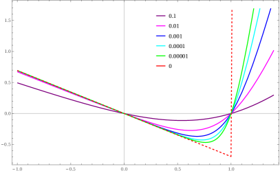
Figure 4: The cumulant generating function $\overline{\chi}^{(\epsilon)}$ as a function of $\alpha/\beta$ for a qubit ($d=2$) at $\epsilon=10^{-k}$ for $k=1,2,3,4,5$. The straight line is the limiting function (23).

Consider now a family of faithful states $\{\rho_{\rm f}^{(\epsilon)}\}_{\epsilon\in]0,1/2[}$ such that $\rho_{\rm f}^{(\epsilon)}$ approaches a pure state $|\psi\rangle\langle\psi|$ as $\epsilon\downarrow 0$. Denote by $\overline{\mathbb{P}}^{(\epsilon)}$ the corresponding heat FS. Without loss of generality, we can assume that $1-\epsilon$ is an eigenvalue of $\rho_{\rm f}^{(\epsilon)}$ (with eigenvector $\psi$). Then, this eigenvalue is simple and the rest of the spectrum of $\rho_{\rm f}^{(\epsilon)}$ is contained in the interval $]0,\epsilon[$. Eq. (20) yields

$$\lim_{\epsilon\downarrow 0}\overline{\varphi}^{(\epsilon)}(\alpha)=\lim_{\epsilon\downarrow 0}d^{\mathrm{i}\frac{\alpha}{\beta}}{\rm tr}\left({\rho_{\rm f}^{(\epsilon)}}^{1+\mathrm{i}\frac{\alpha}{\beta}}\right)=d^{\mathrm{i}\frac{\alpha}{\beta}},$$

which, invoking once again Levy’s theorem, implies that $\overline{\mathbb{P}}^{(\epsilon)}$ converges weakly to the Dirac mass at $\beta^{-1}\log d$. Thus, in the perfect erasure limit, the heat does not fluctuate either, and takes the value imposed by the Landauer bound with probability one. However, any practical implementation of the erasure process will involve some errors and the final pure state $\psi$ will only be reached within some precision $\epsilon>0$ (or with some probability $1-\epsilon$). It is therefore worth paying some attention to the asymptotics $\epsilon\downarrow 0$. In this limit, one easily shows that

$$\langle\Delta Q\rangle={\beta}^{-1}\log d+{\cal O}(\epsilon\log\epsilon),$$

while for $n\geq 2$, Eq. (22) gives

$$\langle\langle\Delta Q^{n}\rangle\rangle={\cal O}(\epsilon(\log\epsilon)^{n}).$$

The presence of powers of $\log\epsilon$ in these formulas is the signature of the singularity developed by the cumulant generating function (see Figure 4)

$$\lim_{\epsilon\downarrow 0}\overline{\chi}^{(\epsilon)}(\alpha)=\lim_{\epsilon\downarrow 0}\log\left(d^{-\frac{\alpha}{\beta}}{\rm tr}\left({\rho_{\rm f}^{(\epsilon)}}^{1-\frac{\alpha}{\beta}}\right)\right)=\begin{cases}-\frac{\alpha}{\beta}\log d&\mbox{if }\alpha<\beta,\\ 0&\mbox{if }\alpha=\beta,\\ \infty&\mbox{if }\alpha>\beta.\end{cases}$$ (23)

For small values of $\epsilon$, $d-1$ of the (repeated) eigenvalues of $\rho_{\rm f}^{(\epsilon)}$ are clustered near zero and the corresponding heat quanta become strongly negative. Accordingly, the system ${\cal S}$ might occasionally absorb large amounts of heat $-Q_{k}^{(\epsilon)}\sim-\beta^{-1}\log\epsilon$. Such heat release by the reservoir corresponds to a transition of ${\cal S}$ to an eigenstate $\phi_{k}$ of $\rho_{\rm f}^{(\epsilon)}$ such that $\langle\phi_{k}|\rho_{\rm f}^{(\epsilon)}\phi_{k}\rangle={\cal O}(\epsilon)\ll 1$, i.e., to a failure of the erasure process to reach the pure state $\psi$. This transition happens at a high energy cost. Thus, it is not surprising that the fluctuations breaking Landauer’s Principle have a total probability $\overline{\mathbb{P}}^{(\epsilon)}(\Delta Q\leq 0)=\epsilon$ which is exponentially small w.r.t. the energy scale $-\log\epsilon$ involved in the process. Still we expect these fluctuations might be relevant in the experimental investigation of the Landauer limit for quantum systems.

As an alternative approach to the analysis of perfect erasure, let us compute the probability distribution of the released heat conditioned on the fact that a final measurement of the system state confirms the success of the erasure process. Applying Bayes rule we derive, for finite $L$ and $T$,

$$\mathbb{P}^{(T,L)}_{\rm success}(\Delta Q)=\sum_{e^{\prime}-e=\Delta Q}\frac{{\rm tr}\left(P^{(L)}_{e^{\prime}}U_{1}^{(T,L)}P^{(L)}_{e}\eta^{(L)}_{i}U_{1}^{(T,L)\ast}P^{(L)}_{e^{\prime}}P_{\rm success}\right)}{{\rm tr}\left(U_{1}^{(T,L)}\eta^{(L)}_{i}U_{1}^{(T,L)\ast}P_{\rm success}\right)},$$

where $P_{\rm success}=|\psi\rangle\langle\psi|\otimes I$ denotes the orthogonal projection on the target pure state $\psi$. Since this projection commutes with $P_{e^{\prime}}^{(L)}$, the corresponding cumulant generating function reads

$$\chi^{(T,L)}_{\rm success}(\alpha)=\log\left(\frac{{\rm tr}\left({\rm e}^{-\alpha H_{\cal R}^{(L)}}U_{1}^{(T,L)}{\rm e}^{\alpha H_{\cal R}^{(L)}}\eta^{(L)}_{i}U_{1}^{(T,L)\ast}P_{\rm success}\right)}{{\rm tr}\left(U_{1}^{(T,L)}\eta^{(L)}_{i}U_{1}^{(T,L)\ast}P_{\rm success}\right)}\right).$$

Proceeding as before, we easily obtain the following expression of the conditional cumulant generating function of heat in the thermodynamic and adiabatic limits and for the target state $\rho_{\rm f}^{(\epsilon)}$,

$$\chi^{(\epsilon)}_{\rm success}(\alpha)=\lim_{T\to\infty}\lim_{L\to\infty}\chi^{(T,L)}_{\rm success}(\alpha)=-\frac{\alpha}{\beta}(\log d+\log(1-\epsilon)).$$

Thus, conditioning on the success of perfect erasure yields a heat distribution which concentrates on

$$\beta\Delta Q=\log\left(p_{\rm max}d\right)<\Delta S,$$

where $p_{\rm max}=1-\epsilon$ denotes the largest eigenvalue of $\rho_{\rm f}^{(\epsilon)}$. Again, such a departure from Landauer principle could in principle be checked experimentally.

5 Conclusion

We have studied the statistics of the heat dissipated in a thermal bath during the quasi-static realization of a Landauer erasure which transforms a completely mixed initial state into a faithful final state $\rho_{\rm f}$. We have shown that the dissipated heat is quantized, and interpreted this phenomenon as a fine version of reversibility for isothermal processes. In the singular limit, when $\rho_{\rm f}$ is close to a pure state $|\psi\rangle\langle\psi|$, the heat distribution acquires extreme outliers. With a small but non-zero probability a large amount of heat can be absorbed by the system during the erasure process. This singularity can be detected in the divergence, Eq. (6), of the moment generating function of the heat Full Statistics and corresponds to a failure of the process to reach the pure state $\psi$. Alternatively, conditioning on the success of the perfect erasure process yields a heat distribution which is concentrated on a value strictly smaller that Landauer’s limit.

We believe this departure could be experimentally detected in a quantum analog of the experiments confirming Landauer’s Principle [SLKL, PBVN, Ra, TSU, BAP]. Several interferometry and control protocols to measure the heat Full Statistics using an ancilla coupled to the joint system ${\cal S}+{\cal R}$ were proposed [CBK, DCH, GPoM, MDCP, RCP]. The proposal of Dorner et al. [DCH] seems to be the most appropriate for our model since it involves only local interactions between the ancilla and the reservoir.

Acknowledgment. The research of T.B. was partly supported by ANR project RMTQIT (Grant No. ANR-12-IS01-0001-01) and by ANR contract ANR-14-CE25-0003-0. The research of V.J. was partly supported by NSERC. A part of this work has been done during a visit of T.B. and M.F. to McGill University partly supported by NSERC. The work of C.-A.P. has been carried out in the framework of the Labex Archimède (ANR-11-LABX-0033) and of the A*MIDEX project (ANR-11-IDEX-0001-02), funded by the “Investisements d’Avenir” French Government program managed by the French National Research Agency (ANR).

References

- [ABGK] Avron, J.E., Bachmann, S., Graf, G.-M., and Klich, I.: Fredholm determinants and the statistics of charge transport. Commun. Math. Phys. 280, 807–829 (2008).
- [AE] Avron, J.E., and Elgart, A.: Adiabatic theorem without a gap condition. Commun. Math. Phys. 203, 445–463 (1999).
- [AFGG] Avron, J.E., Fraas, M., Graf, G.-M., and Grech, P. Adiabatic theorems for generators of contracting evolutions. Commun. Math. Phys. 314, 163–191 (2012).
- [AJPP1] Aschbacher, W., Jakšić, V., Pautrat, Y., and Pillet, C.-A.: Topics in non-equilibrium quantum statistical mechanics. In Open Quantum Systems III. Recent Developments. Lecture Notes in Mathematics Vol. 1882, S. Attal, A. Joye, and C.-A. Pillet editors. Springer, Berlin, 2006.
- [AJPP2] Aschbacher, W., Jakšić, V., Pautrat, Y., and Pillet, C.-A.: Transport properties of quasi-free Fermions. J. Math. Phys. 48, 032101 (2007).
- [AM] Aizenstadt, V.V., and Malyshev, V.A.: Spin interaction with an ideal Fermi gas. J. Stat. Phys. 48, 51–68 (1987).
- [ASF1] Abou-Salem, W.K., and Fröhlich, J.: Adiabatic theorems and reversible isothermal processes. Lett. Math. Phys. 72, 153–163 (2005).
- [ASF2] Abou-Salem, W.K., and Fröhlich, J.: Status of the Fundamental Laws of Thermodynamics. J. Stat. Phys. 126, 1045–1068 (2007).
- [BAP] Bérut, A., Arakelyan, A., Petrosyan, A., Ciliberto, S., Dillenschneider, R. and Lutz, E.: Experimental verification of landauer’s principle linking information and thermodynamics. Nature 483, 187–189 (2012).
- [Be] Bennett, C.H.: Demons, engines and the second law. Scientific American 257, 108–116 (1987).
- [BF] Born, M., and Fock, V.: Beweis des Adiabatensatzes. Z. für Physik 51, 165–180 (1928).
- [BFS] Bach, V., Fröhlich, J., and Sigal, I.M.: Return to equilibrium. J. Math. Phys. 41, 3985–4060 (2000).
- [Bi] Bilingsley, P.: Convergence of Probability Measures. Willey, New York (1968).
- [BFJP] Benoist, T., Fraas, M., Jakšić, V., and Pillet, C.-A.: Adiabatic theorem in quantum statistical mechanics. In preparation, 2016.
- [BoM] Botvich, D.D., and Malyshev, V.A.: Unitary equivalence of temperature dynamics for ideal and locally perturbed Fermi-gas. Commun. Math. Phys. 91, 301–312 (1983).
- [BM] Bhattacharyya, K., and Mukherjee, D.: On estimates of the quantum recurrence time. J. Chem. Phys. 84, 3212–3214 (1986).
- [BR1] Bratteli, O., and Robinson, D.W.: Operator Algebras and Quantum Statistical Mechanics I. Second Edition. Springer, Berlin, 1987.
- [BR2] Bratteli, O., and Robinson, D.W.: Operator Algebras and Quantum Statistical Mechanics II. Second Edition. Springer, Berlin, 1997.
- [CBK] Campisi, M., Blattmann, R., Kohler, S., Zueco, D., and Hänggi, P.: Employing circuit qed to measure non-equilibrium work fluctuations. New J. Phys. 15, 105028 (2013).
- [CJ] Crooks, G.E., and Jarzynski, C.: Work distribution for the adiabatic compression of a dilute and interacting classical gas. Phys. Rev. E 75, 021116 (2007).
- [Cr] Crooks, G.E.: Entropy production fluctuation theorem and the nonequilibrium work relation for free energy differences. Phys. Rev. E 60, 2721 (1999).
- [CV] Campos Venuti, L.: The recurrence time in quantum mechanics. Preprint \htmladdnormallinkarXiv:1509.04352http://arxiv.org/abs/1509.04352, (2015).
- [DCH] Dorner, R., Clark, S.R., Heaney, L., Fazio, R., Goold, J. and Vedral, V.: Extracting quantum work statistics and fluctuation theorems by single-qubit interferometry. Phys. Rev. Lett. 110, 230601 (2013).
- [DJ] Dereziński, J., and Jakšić, V.: Return to equilibrium for Pauli-Fierz systems. Ann. Henri Poincaré 4, 739–793 (2003).
- [DL] Dillenschneider, R., and Lutz, E.: Memory erasure in small systems. Phys. Rev. Lett. 102, 210601 (2009).
- [dRK] de Roeck, W., and Kupianien, A.: Return to equilibrium for weakly coupled quantum systems: A simple polymer expansion. Commun. Math. Phys. 305, 797–826 (2011).
- [DS] Davies, E.B., and Spohn, H.: Open quantum systems with time-dependent Hamiltonians and their linear response. J. Stat. Phys. 19, 511–523 (1978).
- [ECM] Evans, D.J., Cohen, E.G.D., and Morriss, G.P:. Probability of second law violations in shearing steady states. Phys. Rev. Lett. 71, 2401 (1993).
- [FM] Fröhlich, J., and Merkli, M.: Another return of “Return to Equilibrium”. Commun. Math. Phys. 251, 235–262 (2004).
- [FMSU] Fröhlich, J., Merkli, M., Schwarz, S., and Ueltschi, D.: Statistical mechanics of thermodynamic processes. In A Garden of Quanta: Essays in Honor of Hiroshi Ezawa, J. Arafune, A. Arai, M. Kobayashi, K. Nakamura, T. Nakamura, I. Ojima, N. Sakai, A. Tonomura, and K. Watanabe editors. World Scientific Publishing, Singapore, 2003.
- [FMU] Fröhlich, J., Merkli, M., and Ueltschi, D.: Dissipative transport: Thermal contacts and tunneling junctions. Ann. Henri Poincaré 4, 897–945 (2003).
- [HJPR] Hanson, E., Joye, A., Pautrat, Y., and Raquépas, R.: Landauer’s principle in repeated interaction systems. Preprint \htmladdnormallink arXiv:1510.00533 [math-ph]http://arxiv.org/abs/1510.00533 (2015).
- [GC] Gallavotti, G., and Cohen, E.G.D.: Dynamical ensembles in nonequilibrium statistical mechanics. Phys. Rev. Lett. 74, 2694 (1995).
- [GPaM] Goold, J., Paternostro, M., and Modi, K.: Nonequilibrium quantum Landauer principle. Phys. Rev. Lett. 114, 060602 (2015).
- [GPoM] Goold, J., Poschinger, U., and Modi, K.: Measuring the heat exchange of a quantum process. Phys. Rev. E 90, 020101 (2014).
- [Ja] Jarzynski, C.: Nonequilibrium equality for free energy differences. Phys. Rev. Lett. 78, 2690 (1997).
- [JKP] Jakšić, V., Kritchevski, E., and Pillet C.-A.: Mathematical theory of the Wigner-Weisskopf atom. Large Coulomb Systems. Lecture Notes on Mathematical Aspects of QED. Lecture Notes in Physics 695, 147-218 (2006).
- [JOP1] Jakšić, V., Ogata, Y., and Pillet, C.-A.: The Green-Kubo formula for the spin-fermion system. Commun. Math. Phys. 268, 369–401 (2006).
- [JOP2] Jakšić, V., Ogata, Y., and Pillet, C.-A.: The Green-Kubo formula for locally interacting fermionic open systems. Ann. Henri Poincaré 8, 1013–1036 (2007).
- [JOPP] Jakšić, V., Ogata, Y., Pautrat, Y., and Pillet, C.-A.: Entropic fluctuations in quantum statistical mechanics – an introduction. In Quantum Theory from Small to Large Scales, J. Fröhlich, M. Salmhofer, V. Mastropietro, W. de Roeck and L.F. Cugliandolo editors. Oxford University Press, Oxford, 2012.
- [Jo] Joye, A.: General adiabatic evolution with a gap condition. Commun. Math. Phys. 275, 139–162 (2007).
- [JP1] Jakšić, V., and Pillet, C.-A.: On a model for quantum friction III: Ergodic properties of the spin–boson system. Commun. Math. Phys. 178, 627–651 (1996).
- [JP2] Jakšić, V., and Pillet, C.-A.: Non-equilibrium steady states of finite quantum systems coupled to thermal reservoirs. Commun. Math. Phys. 226, 131–162 (2002).
- [JP] Jakšić, V., and Pillet, C.-A.: A note on the Landauer principle in quantum statistical mechanics. J. Math. Phys. 55, 075210 (2014).
- [JPPP] Jakšić, V., Panangaden, J., Panati, A., and Pillet, C.-A.: Energy conservation, counting statistics, and return to equilibrium. Lett. Math. Phys. 105, 917–938 (2015).
- [Ka] Kato, T.: On the adiabatic theorem of quantum mechanics. J. Phys. Soc. Japan 5, 435–439 (1950).
- [Ku] Kurchan, J.: A quantum fluctuation theorem. Preprint \htmladdnormallinkarXiv:cond-mat/0007360http://arxiv.org/abs/cond-mat/0007360 (2000).
- [La] Landauer, R.: The physical nature of information. Phys. Lett. A 217, 188–193 (1996).
- [LC] Lutz, E., and Ciliberto, S.: Information: From Maxwell’s demon to Landauer’s eraser. Physics Today, 68, 30–35 (2015).
- [LL1] Levitov, L.S., and Lesovik, G.B.: Charge-transport statistics in quantum conductors. JETP Lett. 55, 555–559 (1992).
- [LL2] Levitov, L.S., and Lesovik, G.B.: Charge distribution in quantum shot noise. JETP Lett. 58, 230–235 (1993).
- [LLY] Lee, H., Levitov, L.S., and Yakovets, A.Yu.: Universal statistics of transport in disordered conductors. Phys. Rev. B 51, 4079–4083 (1995).
- [MDCP] Mazzola, L., De Chiara, G., and Paternostro, M.: Measuring the characteristic function of the work distribution. Phys. Rev. Lett. 110, 230602 (2013).
- [MMS1] Merkli, M., Mück, M., and Sigal, I.M.: Instability of equilibrium states for coupled heat reservoirs at different temperatures. J. Funct. Anal. 243, 87–120 (2007).
- [MMS2] Merkli, M., Mück, M., and Sigal, I.M.: Theory of non-equilibrium stationary states as a theory of resonances. Ann. Henri Poincaré 8, 1539–1593 (2007).
- [Pe] Pekola, J.P.: Towards quantum thermodynamics in electronic circuits. Nature Physics 11, 118–123 (2015).
- [PGA] Pekola, J.P., Golubev, D.S., Averin, D.V.: Maxwell’s demon based on a single qubit. Phys. Rev. B. 93, 024501 (2016).
- [PBVN] Price, G.N., Bannerman, S.T., Viering, K., Narevicius, E., and Raizen, M.G.: Single-photon atomic cooling. Phys. Rev. Lett. 100, 093004 (2008).
- [Ra] Raizen, M.G.: Comprehensive control of atomic motion. Science 324, 1403–1406 (2009).
- [RCP] Roncaglia, A.J., Cerisola, F., and Paz, J.-P.: Work measurement as a generalized quantum measurement. Phys. Rev. Lett. 113, 250601 (2014).
- [Ru] Ruelle, D.: Statistical Mechanics: Rigorous Results. Benjamin, London, 1977.
- [RW] Reeb, D., and Wolf, M.M.: An improved landauer principle with finite-size corrections. New J. Phys. 16, 103011 (2014).
- [SL] Sarandy, M.S., and Lidar, D.A.: Adiabatic approximation in open quantum systems. Phys. Rev. A 71, 012331 (2005).
- [SLKL] Serreli, V., Lee, C.F., Kay, E.R., and Leigh, D.A.: A molecular information ratchet. Nature 445, 523–527 (2007).
- [SS] Shimizu, A., and Sakaki, H.: Quantum noises in mesoscopic conductors and fundamental limits of quantum interference devices. Phys. Rev. B 44, 13136 (1991).
- [SSS] Silva, J.P.P, Sarthour, R.S., Souza, A.M., Oliveira, I.S., Goold, J., Modi, K., Soares-Pinto, D.O., and Céleri, L.C.: Experimental demonstration of information to energy conversion in a quantum system at the Landauer limit. Preprint \htmladdnormallinkarXiv:1412.6490http://arxiv.org/abs/1412.6490 (2014).
- [Ta] Tasaki, H.: Jarzynski relations for quantum systems and some applications. Preprint \htmladdnormallinkarXiv:cond-mat/0009244http://arxiv.org/abs/cond-mat/0009244 (2000).
- [TAS] Thunström, P., Åberg, J., and Sjöqvist, E.: Adiabatic approximation for weakly open systems. Phys. Rev. A 72, 022328 (2005).
- [Te] Teufel, S.: A note on the adiabatic theorem without gap condition. Lett. Math. Phys. 58, 261–266 (2001).
- [TLH] Talkner, P., Lutz, E., and Hänggi, P.: Fluctuation theorems: Work is not an observable. Phys. Rev. E 75, 050102 (2007).
- [TSU] Toyabe, S., Sagawa, T., Ueda, M., Muneyuki, E., and Sano, M.: Experimental demonstration of information-to-energy conversion and validation of the generalized Jarzynski equality. Nature Physics 6, 988–992 (2010).
- [Wia] \htmladdnormallinkEntropy in thermodynamics and information theory — Wikipedia, the free encyclopedia https://en.wikipedia.org/wiki/Entropy_in_thermodynamics_and_information_theory , 2015. [Online; accessed 29-November-2015].
- [Wib] \htmladdnormallinkMaxwell’s demon — Wikipedia, the free encyclopedia https://en.wikipedia.org/wiki/Maxwell%27s_demon, 2015. [Online; accessed 29-November-2015].