Obliquity Variability of a Potentially Habitable Early Venus

Abstract

Venus currently rotates slowly, with its spin controlled by solid-body and atmospheric thermal tides. However, conditions may have been far different 4 billion years ago, when the Sun was fainter and most of the carbon within Venus could have been in solid form, implying a low-mass atmosphere. We investigate how the obliquity would have varied for a hypothetical rapidly rotating Early Venus. The obliquity variation structure of an ensemble of hypothetical Early Venuses is simpler than that Earth would have if it lacked its large Moon (Lissauer et al., 2012), having just one primary chaotic regime at high prograde obliquities. We note an unexpected long-term variability of up to $\pm 7^{\circ}$ for retrograde Venuses. Low-obliquity Venuses show very low total obliquity variability over billion-year timescales – comparable to that of the real Moon-influenced Earth.

1. Introduction

The obliquity $\Psi$ — defined as the angle between a planet’s rotational angular momentum and its orbital angular momentum — is a fundamental dynamical property of a planet. A planet’s obliquity influences its climate and potential habitability. Varying orbital inclinations and precession of the orbit’s ascending node can alter obliquity, as can torques exerted upon a planet’s equatorial bulge by other planets. The Earth exhibits a relatively stable and benign long-term climate because our planet’s obliquity varies only of order $\sim 3^{\circ}$. As a point of comparison, the obliquity of Mars varies over a very large range — $\sim 0^{\circ}$–$60^{\circ}$ (Touma & Wisdom, 1993; Laskar et al., 1993, 2004).

Changes in obliquity drive changes in planetary climate. In the case where those obliquity changes are rapid and/or large, the resulting climate shifts can be commensurately severe (see, e.g., Armstrong et al., 2004). The Earth’s present climate resides at a tipping point between glaciated and non-glaciated states, and the small $\sim 3^{\circ}$ changes in our obliquity from Milankovic Cycles drives glaciation and deglaciation of northern Europe, Siberia, and North America (Milankovič, 1998). These glacial/interglacial cycles reduce biodiversity in periodically glaciated Arctic regions (e.g., Araújo et al., 2008; Hawkins & Porter, 2003; Hortal et al., 2011). The resulting insolation shifts jolt climatic patterns worldwide, causing species in affected regions to migrate, adapt, or be rendered extinct.

Perhaps paradoxically, large-amplitude obliquity variations can also act to favor a planet’s overall habitability. Low values of obliquity can initiate polar glaciations that can, in the right conditions, expand equatorward to envelop an entire planet like the ill-fated ice-planet Hoth in The Empire Strikes Back (Lucas, 1980). Indeed, our own planet has experienced so-called Snowball Earth states multiple times in its history (Hoffman et al., 1998). Although high obliquity drives severe seasonal variations, the annual average flux at each surface point is more uniform on a high-obliquity world than the equivalent low-obliquity one. Hence high obliquity can act to stave off snowball states (Spiegl et al., 2015) and extreme obliquity variations may act to expand the outer edge of the habitable zone (Armstrong et al., 2014) by preventing permanent snowball states.

Thus knowledge of a planet’s obliquity variations may be critical to the evaluation of whether or not that planet provides a long-term habitable environment. A planet’s siblings affect its obliquity evolution primarily via nodal precession of the planet’s orbit. Obliquity variations become chaotic when the precession period of the planet’s rotational axis (26,000 years for Earth) becomes commensurate with the nodal precession period of the planet’s orbit ($\sim 100,000$ years for Earth). Secular resonances, those that only involve orbit-averaged parameters as opposed to mean-motion resonances for which the orbital periods are near-commensurate, typically cluster together in the Solar System such that if you are near one secular period, you are likely near others as well. And those clusters of secular resonances act to drive chaos that increases the range of a planet’s obliquity variations.

The gravitational influence of Earth’s Moon speeds the precession of our rotation axis, and stabilizes our obliquity. Without this influence Earth’s rotation axis precession would have a period of $\sim 100,000$ years, close enough to commensurability as to drive large and chaotic obliquity variability (Laskar et al., 1993). Though our previous work (Lissauer et al., 2012) showed that such variations would not be as large as those of Mars, the difference between commensurate precessions and non-commensurate precessions is stark.

Atobe & Ida (2007) investigated the obliquity evolution of potentially habitable extrasolar planets with large moons, following on work by (Atobe et al., 2004) showing the generalized influence of nearby giant planets on terrestrial planet obliquity in general. Brasser et al. (2014) studied the obliquity variations in for the specific super-Earth HD40307g.

To expand the general understanding of potentially habitable worlds’ obliquity variations, we use the only planetary system that we know well enough to render our calculations accurate: our own. In this paper, we analyze the obliquity variations of a hypothetical Early Venus as an analog for potentially habitable exoplanets.

Venus was likely in the Sun’s habitable zone 4.5 Gyr ago, when the Sun was only 70% its present luminosity (Sackmann et al., 1993). Such an Early Venus could well have had a low-mass atmosphere (with most of the planet’s carbon residing within rocks), and tides would not yet have substantially damped its spin rate. In fact, Abe et al. (2011) suggest that the real Venus may have been habitable as recently as 1 Gyr ago, provided that its initial water content was small (as might result from impact-driven dessication, as per Kurosawa (2015), or because the planet is located well interior to the ice line).

Rotation	LR93a		CLS03		Lissauer et al. (2012)
Period (hr)	$J_{2}$	('' /yr)	$J_{2}$	('' /yr)	J2	('' /yr)
4	1.405422e-02	99.94621	4.694002e-02	334.75028	4.692702e-02	334.63436
8	3.504570e-03	49.84532	1.036030e-02	147.76787	1.034730e-02	147.57222
12	1.555255e-03	33.18048	4.526853e-03	96.84904	4.513853e-03	96.56422
16	8.739020e-04	24.85893	2.536138e-03	72.34533	2.523138e-03	71.96950
20	5.588364e-04	19.87076	1.623182e-03	57.87820	1.610182e-03	57.41067
24	3.878196e-04	16.54781	1.129453e-03	48.32779	1.116453e-03	47.76823
30	2.480000e-04	13.22734	7.266291e-04	38.86438	7.136291e-04	38.16642
36	1.721063e-04	11.01537	5.082374e-04	32.62021	4.952374e-04	31.78363

Table 1Values for the zonal harmonic ($J_{2}$) and ‘precession’ constant ($\alpha$) determined from the rotation period for the models presented in Laskar & Robutel (1993), Correia et al. (2003), and Lissauer et al. (2012).

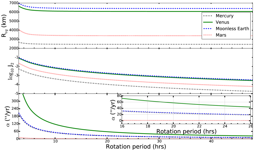
Figure 1.— Illustration of how the derived starting values for the equatorial radius due to rotation (R_eq), zonal harmonic (J₂), and ‘precession’ constant ($\alpha$) vary in response to the initial rotation period from 4 to 48 hrs using the formalism given by Lissauer et al. (2012). Curves are provided considering each of the terrestrial planets (Mercury, Venus, Moonless Earth (a single planet with the mass of the Moon added to that of the Earth), and Mars).

In this work we numerically explore the obliquity variations of Early Venus with a parameter grid study that incorporates a wide variety of rotation rates and obliquities. Note that this work is not intended to study Venus’ actual historical obliquity state, information about which has been destroyed by its present tidal equilibrium (Correia et al., 2003; Correia & Laskar, 2003). Instead, we use Venus with a wide range of assigned rotation rates and initial obliquities as an analog for habitable exoplanets and to explore what types of obliquity behavior were possible for a potentially habitable Early Venus. Our methods build on those of Lissauer et al. (2012) and are described in Section 2. We provide qualitative and quantitative descriptions of the drives of obliquity variations and chaos in Section 3. Results of our simulations are presented in Section 4, and we conclude in Section 5. Readers interested primarily in the results might consider jumping to Section 4, while those also interested in the physics of why obliquity varies can add Section 3.

2. Methodology

2.1. Approach

We track the evolution of obliquity for the hypothetical Venus computationally, using a modified version of the mixed-variable sympletic (MVS) integration algorithm within the mercury package developed by Chambers (1999). The modified algorithm smercury (for spin-tracking mercury) explicitly calculates both orbital forcing for the 8-planet Solar System and spin torques on one particular planet in the system from the Sun and sibling planets following Touma & Wisdom (1994). Our explicit numerical integrations represent an approach distinct from the frequency-mapping treatment employed by Laskar et al. (1993). See Lissauer et al. (2012) for a complete mathematical description of our computational techniques.

The smercury algorithm treats the putative Venus as an axisymmetric body. In so doing, we neglect both gravitational and atmospheric tides. Tidal influence critically drives the present-day rotation state of real Venus (Correia & Laskar, 2001). We are interested in an early stage of dynamical evolution, however, where the tidal effects do not dominate. Therefore we consider only solar and interplantary torques on the rotational bulge. The simultaneous consideration of tidal and dynamical effects is outside the scope of the present work.

In the case of differing rotation periods, we incorporate the planet’s dynamical oblateness and its effects on the planet’s gravitational field. These effects manifest as the planet’s gravitational coefficient $J_{2}$, values for which we determine from the Darwin-Radau relation, following Appendix A of Lissauer et al. (2012). Additionally, as in Lissauer et al. (2012) we employ “ghost planets” to increase the efficiency of our calculations — essentially we calculate planetary orbits just one time, while assuming a variety of different hypothetical Venuses for which we calculate just the obliquity variations. We neglect (the very small effects of) general relativity and stellar $J_{2}$.

2.2. Initial Conditions

We select orbital initial conditions with respect to the J2000 epoch where the Earth-Moon barycenter resides coplanar with the ecliptic. Li & Batygin (2014b) and Brasser & Walsh (2011) investigated how obliquity variations are affected by alternate early Solar System architectures, specifically the Nice model (Morbidelli et al., 2007). As an investigation of the long-term characteristic obliquity behavior, however, we instead elect to integrate the present Solar System orbits, which are known to much higher accuracy.

Lissauer et al. (2012) showed that chaotic variations in obliquity for a Moonless Earth can manifest from slightly different initial orbits. We thus remove this effect by using a common orbital solution for all of our simulations. We assume the density of our hypothetical Venus to be the same as the real Venus, 5.204 g/cm³. However, we assume a moment of inertia coefficient to be the same as that for the real Earth (0.3296108; Ahrens, 1995) given that a truly habitable Venus would likely have a different internal structure than the real one. We do not vary the moment of inertia with rotation period.

We consider a range of rotation periods of between 4 and 36 hours. The short end is set by the rotation speed at which the planet would be near breakup, where our Darwin-Radau and axisymmetric assumptions break down. The longer limit represents a value 50% longer than Earth’s rotation, which itself has been tidally slowed over the past 4.5 Gyr. In the epoch of Solar System history that we consider, Earth’s own day was significantly shorter than it is today.

Along with various rotation rates, we also consider initial obliquity values $\Psi$ that range from $0^{\circ}$ to $180^{\circ}$. Planets with obliquity between $90^{\circ}$ and $180^{\circ}$ rotate retrograde to their orbital motions. Obliquity alone does not completely determine the orientation of a planet’s spin axis in space (unless $\Psi=0^{\circ}$ or $\Psi=180^{\circ}$). Therefore, for each obliquity we also consider various initial axis azimuths, $\varphi$, which correspond to the direction that the spin pole points.

In order to generate the proper initial spin states, we define the angles of obliquity and azimuth. Lissauer et al. (2012) used a similar approach; however, that previous study was for the Earth-Moon barycenter with zero initial inclination relative to the ecliptic plane. In contrast, the definition of spin direction for any other planet requires two additional rotations that include that planet’s inclination, $i$, and its ascending node, $\Omega$, both relative to the J2000 ecliptic. Thus the general rotation matrices $R_{1}$ and $R_{2}$ can be used to define the desired obliquity, $\Psi$, and azimuth, $\varphi$:

$$R_{1}(\gamma)=\begin{pmatrix}1&0&0\\ 0&\cos\gamma&-\sin\gamma\\ 0&\sin\gamma&\cos\gamma\end{pmatrix}{\rm and\;\;}R_{2}(\beta)=\begin{pmatrix}\cos\beta&\sin\beta&0\\ -\sin\beta&\cos\beta&0\\ 0&0&1\\ \end{pmatrix}{\rm~{}~{}~{}~{}~{}.}$$ (1)

The azimuthal angles, $\varphi$ and $\Omega$, undergo rotations via $R_{2}$ with $\beta=\varphi$ or $\beta=\Omega$, where the altitudinal angles are rotated using $R_{1}$ with $\gamma=\Psi$ and $\gamma=i$.

3. Obliquity Evolution

A planet’s obliquity, $\Psi$, is defined as the magnitude of the angular distance between the direction of the angular momentum vector for a planet’s spin and that for its orbit. Therefore obliquity can change if either of those two vectors change direction: (1) the rotational angular momentum vector or (2) the orbital angular momentum vector. Let’s consider each in turn.

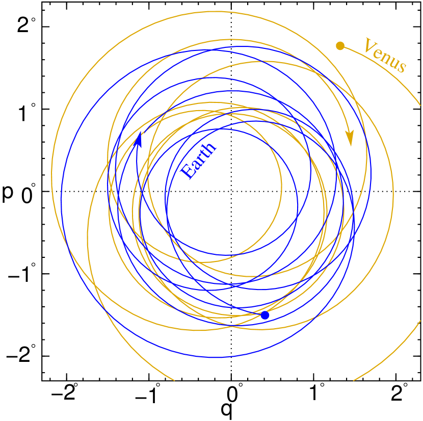
Figure 2.— This plot shows the projected direction in which Venus’ (yellow) and Earth’s (blue) orbital angular momentum points as it varies over the course of 500,000 years from the present day. The projection is in $p$-$q$ space, with $p\equiv I\sin(\Omega)$ and $q\equiv I\cos(\Omega)$ where $\Omega$ is the longitude of the ascending node of the orbit and $I$ is the orbital inclination. The indicated motion represents nodal precession, where a planet’s orbit reorients in space like a coin spinning down on a desktop.

3.1. Rotational Angular Momentum

Torques on a planet’s rotational bulge from the Sun primarily drive changes in the direction of that planet’s rotational axis. Because the star must always be located within the plane of the planet’s orbit, however, these changes cannot directly alter the planet’s obliquity $\Psi$. Instead, the stellar torque induces the planetary rotation axis to precess around the orbit normal, constantly changing the axis azimuth $\varphi$, but leaving the obliquity $\Psi$ unchanged. This effect is called the precession of the equinoxes. It is why the date of the equinox slowly creeps forward over time, and why Polaris has not always been near the Earth’s north pole (see, e.g., Karttunen, 2007).

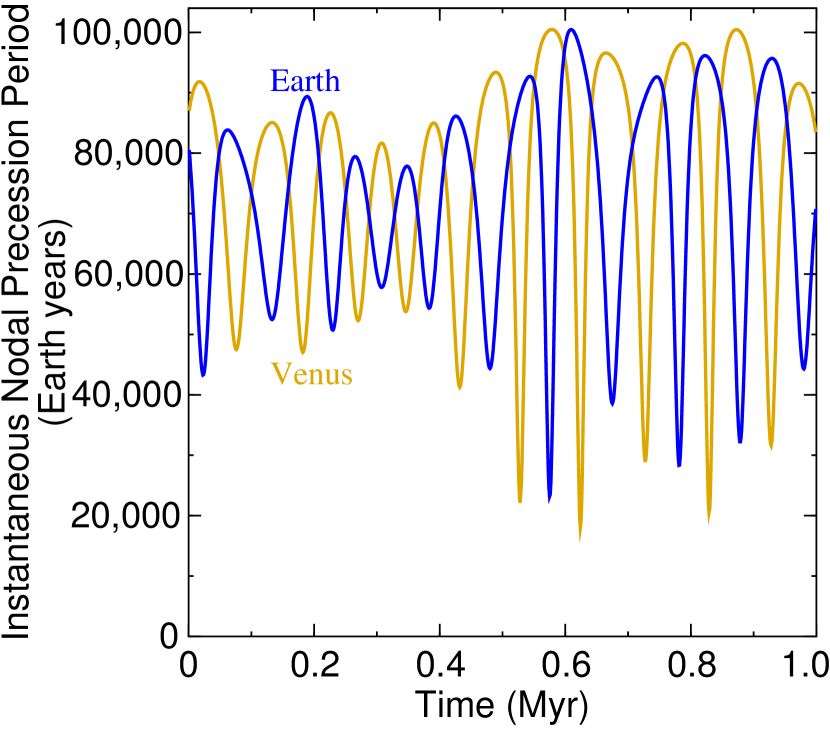
Figure 3.— While Figure 2 shows the direction that the orbit poles of Venus and Earth point to, it lacks a timescale. This plot provides such a timescale, as it depicts the instantaneous precession period (i.e., $2\pi/\frac{\mathrm{d}\varphi}{\mathrm{d}t}$ for both Venus (yellow) and Earth (blue) over a million years. Because Venus and Earth each represent the primary influence on the nodal precession of the other and because they are of comparable mass, the long-term average precession rates for the two are about the same at $\sim 70,000$ years.

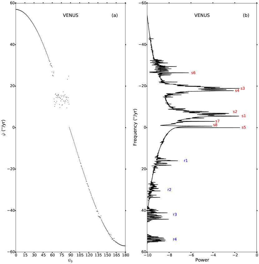
Figure 4.— Precession frequencies (a) for a hypothetical Venus with a rotation period of 20 hours. Panel (a) shows the average precession rate $\dot{\varphi}$ as a function of initial obliquity $\Psi_{0}$. Chaotic zones appear for obliquities ranging from 60${}^{\circ}-90^{\circ}$ that correlates to the precession frequencies ranging from 0 – 26''/yr showing correspondence with the main secular orbital frequencies (b) of the Solar System (Laskar & Robutel, 1993; Laskar, 1996). The power shown in the $x$-axis of panel (b) is logarithmic.

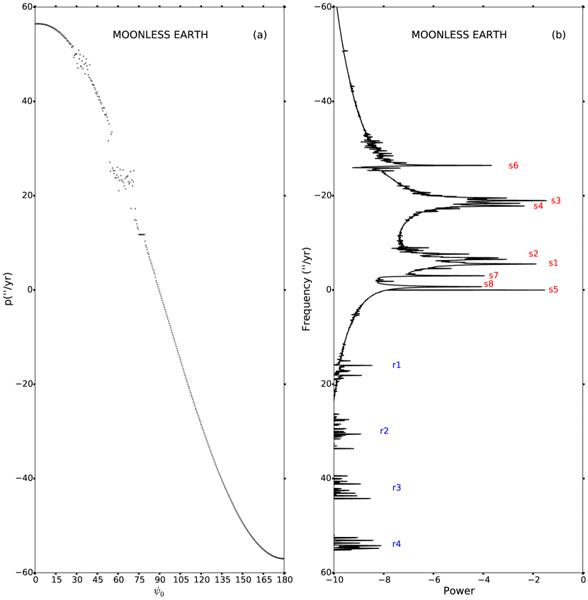
Figure 5.— Similar to Figure 4, here we show the precession frequencies (a) and the power spectrum of the orbital angular momentum vector (b) for a 24-hour-rotation Moonless Earth for comparison with our hypothetical Venuses.

The rate of axial precession depends on the planet’s dynamical oblateness gravitational coefficient $J_{2}$, the mass and distance from the Sun, and the planet’s moment of inertia. The rate also depends weakly on the obliquity itself; therefore precession rates are typically given in terms of the precession constant $\alpha$, where

$$\dot{\varphi}=\alpha\cos(\Psi)~{}~{}~{}~{}.$$ (2)

In Table 1 we show the values of Venus’ zonal harmonic ($J_{2}$) and precession constant ($\alpha$) for both the present study and previous work for a range of rotation periods. Our values strongly resemble those of Correia et al. (2003) but differ substantially from those used by Laskar & Robutel (1993). Figure 1 grapically represents the equatorial radius, $J_{2}$, and precession constant $\alpha$ for our hypothetical Early Venuses as a function of their rotation period.

In general, axial precession for Venus occurs about twice as fast as axial precession for an equivalent planet at 1 AU. Because the Sun’s gravity drives axial precession, the fact that Venus’ semimajor axis is nearly $\sqrt{2}$ AU explains the factor of 2 faster axial precession. Functionally, for obliquity variations, the Sun speeds Venus’ axial precession in a similar manner that the Moon speeds Earth’s.

An expectation might be that Early Venus’ obliquity variations should more closely resemble that of real-life Earth with the Moon than that of the moonless Earth from Lissauer et al. (2012). Circumstances that act to slow Venus’ axial precession from that of the precession constant — such as a smaller rotational bulge, or a higher obliquity — could act to bring the axial precession rate into near-commensurability with precession rates of the orbital ascending node, leading to chaotic obliquity evolution.

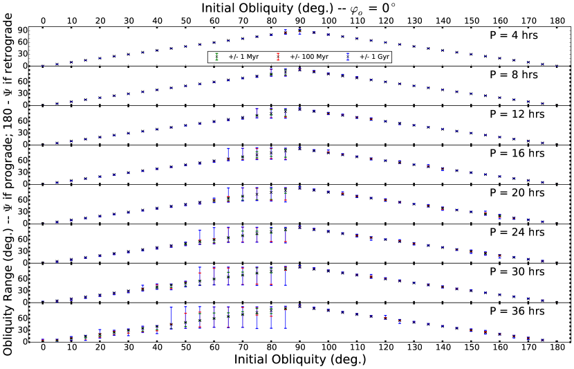
Figure 6.— Obliquity variation of a hypothetical young Venus considering for various initial obliquities ($\Psi$) and rotation periods (P). We calculate the variations for two different initial azimuths: $\varphi_{0}=0^{\circ}$ is shown here, and $\varphi_{0}=180^{\circ}$ is shown in Figure 7. The colored bars indicate the range of obliquity variation over $\pm 1$ Myr (green), $\pm 100$ Myr (red), and $\pm 1$ Gyr (blue). Obliquities greater than 90^∘ are considered to spin in retrograde and those less than 90^∘ are prograde relative to the orbital motion. The largest variations occur for high prograde initial obliquity, with the larger variations extending to lower initial obliquity for slower rotation. Some initially high prograde obliquities obtain retrograde rotation, but they do so temporarily, with a maximum obliquity of $\sim 95^{\circ}$.

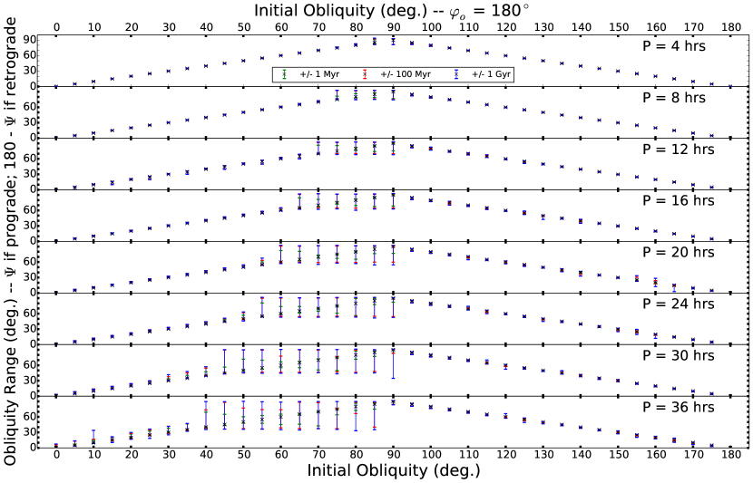
Figure 7.— Same as Figure 6, but for $\varphi=180^{\circ}$.

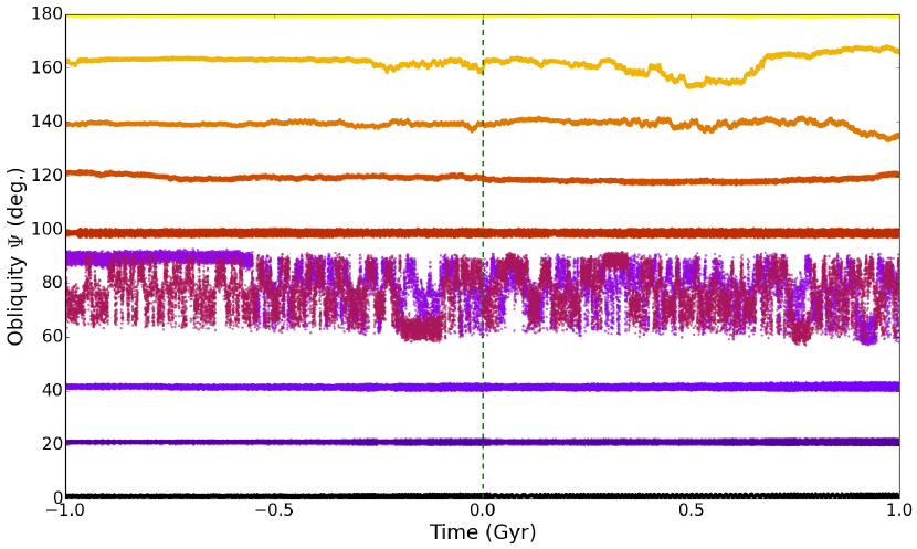
Figure 8.— Variations of hypothetical Venus’s obliquity 1 Gyr into the future and past for a range of initial obliquities with an initial 20 hour rotation period and initial azimuth of 180^∘. The initial obliquities are from $0^{\circ}-180^{\circ}$ for increments of 20^∘ and have been color-coded to distinguish between overlapping regions.

3.2. Orbital Angular Momentum

In a single-planet system, neglecting tidal effects and those of stellar oblateness, a planet’s rotational axis would merrily precess around in azimuth $\varphi$ at a constant rate, but its obliquity $\Psi$ would never change because the orbit plane would remain fixed. Thus an important mechanism for altering planetary obliquity involves the evolution of the orbit. Because obliquity is the relative angle between the rotation axis and the orbit normal, either changes in the direction that the axis points in space or changes in the direction of the orbit normal can each alter obliquity (see, for instance, Armstrong et al., 2014, Figure 1).

We illustrate the evolution of the orbit planes of both Venus and Earth from an analytical, secular calculation in Figure 2. Figure 2 shows the variations in direction of the orbital angular momentum vectors over 500,000 years. The motions are of similar magnitude. Because Earth and Venus have similar masses and because they each provide the primary influence on the orbital evolution of the other (e.g., Murray & Dermott, 2000), their orbital precessions are qualitatively similar. Interestingly, Mercury drives the second most important influence on both Venus and Earth owing to its high orbital inclination relative to both the ecliptic (the plane of Earth’s orbit) and the invariable plane (the plane of the net angular momentum of the entire Solar System).

The orbital variations of Venus and Earth involve some changes in the orbital inclination of the two planets, represented by the distance of the lines in Figure 2 from the origin. The primary effect, though, is counterclockwise near-circular changes that correspond to the precession of the orbit through space. We call that effect nodal precession, as it drives monotonic increases in the element known as the orbit’s ascending node, the angle at which the planet comes up through the reference plane from below.

We show the effective period of the nodal precession of the orbits of Venus and Earth in Figure 3. Although the precession rate changes as the orbit inclinations of each planet vary, the long-term average precession rate for both planets is in the vicinity of $\sim 70,000$ years.

3.3. Spin Chaos

Through the integration of a secular solution and frequency analysis, Laskar & Robutel (1993) and Laskar (1996) showed that chaos can be induced when the axial (spin) precessional frequencies are commensurate with the secular eigenmodes of the Solar System (the drivers of nodal precession). Specifically when the spin precession frequency crosses the eigenmodes associated with secular frequencies $s$1 – $s$8 ($0-26$''/ yr) that are associated with orbital variations of the planets (including nodal precession), chaotic obliquity evolution can result. As a result of this interaction, the obliquity of our hypothetical Venus can vary substantially. Weaker secular frequency eigenmodes can produce additional chaotic zones, albeit smaller in amplitude and potentially with a longer timescale to develop (e.g., Li & Batygin, 2014a).

Figure 4a illustrates the chaotic zones as a function of initial obliquity $\Psi_{0}$ for a hypothetical Venus with a 20-hr rotation period. The $y$-axis represents the actual average axial (spin) precession rate $\dot{\varphi}$ in arcseconds per year. Positive rates here correspond to clockwise precession as viewed from above the orbit normal; negative rates correspond to counterclockwise precession, as occurs for obliquities $\Psi>90^{\circ}$ (retrograde rotation).

In general the curve of precession rates in Figure 4a varies as a smooth cosine from $+\alpha$ to $-\alpha$, as expected from Equation 2. However between $\sim 0$''/yr  and $26$''/yr  the obliquity becomes chaotic, ranging freely over this span as a function of time regardless of where in that region the initial obliquity would place it. For this rotation rate, the primary chaotic obliquity zone ranges from $\Psi\sim 60^{\circ}$ to $\Psi=90^{\circ}$.

The power spectrum of the orbit angular momentum direction vector (like that shown in Figure 2) is shown in Figure 4b. The peaks in this power spectrum labeled $s$1-$s$8 correspond to known Solar System secular eigenfrequencies that result from the 8 interacting Solar System planets. The secular eigenfrequencies bracket the $0$''/yr-$26$''/yr  chaos region for the 20-hour-rotation Venus, correlating with the chaotic zones in Figure 4a. The areas labeled $r$1-$r$4 are clusters of lower-grade retrograde peaks in the frequency power spectrum that we will discuss further in Section 4.2.3.

We show a similar plot for a 24-hour-rotation Moonless Earth in Figure 5 for comparison. The Moonless Earth plot shows the previously known chaotic regions in $\dot{\varphi}$ space, though their correlation with the secular eigenfrequences is poorer than the hypothetical 20-hour-rotation Venus case. Li & Batygin (2014a) showed that while the chaotic range of obliquities for a Moonless Earth does indeed extend from $\Psi=0^{\circ}$ up to $\Psi\sim 85^{\circ}$, the chaotic behavior is not uniform throughout that range.

In fact, Li & Batygin (2014a) find two separate and independent major chaotic zones: one from $\Psi=0^{\circ}$ to $\Psi=45^{\circ}$, and one from $\Psi=65^{\circ}$ to $\Psi=85^{\circ}$. While the region between these two major zones is also chaotic, it is only weakly chaotic. That connecting region serves as a narrow ‘bridge’ across which it is possible for planets to traverse, though only with substantially reduced probability (Li & Batygin, 2014a).

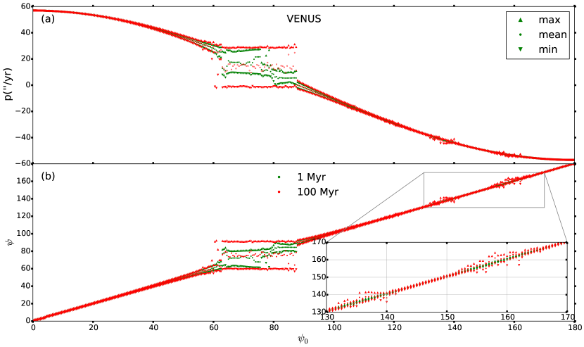
Figure 9.— Maximum, mean, and minimum variations designated by the up-triangle, filled circle, and down triangle, respectively, in (a) the precession constant and (b) the obliquity for a hypothetical Venus with a 20 hr rotation period. The points are color coded to signify how the parameters change over 1 Myr (green) and 100 Myr (red). The inset in (b) shows potential chaotic zones that appear to be present in small ranges of retrograde obliquity.

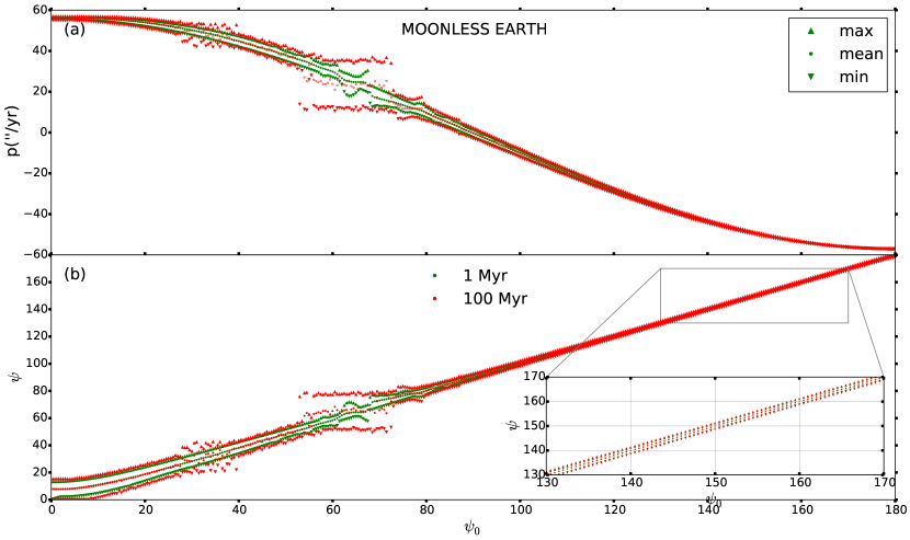
Figure 10.— Similar to Figure 9, here we plot similar maximum, mean, and minimum extents of variation in obliquity $\Psi$, but this time for a 24-hour-rotation-period Moonless Earth. This plot verifies the lower-resolution integrations presented in Lissauer et al. (2012) in that, unlike for hypothetical early Venus, no chaotic obliquity variations are evident in any of the retrograde Moonless Earth cases.

4. Numerical Results

4.1. Coarse Grid

We initially explore the obliquity of hypothetical Early Venuses by numerically integrating the obliquity variations forward to +1 Gyr and backward to -1 Gyr over a coarse grid of rotation rates and initial obliquities. We show a summary of the resulting obliquity variations as a function of initial obliquity and rotation rate in Figures 6 and 7. The difference between the two figures is the azimuthal direction in which the rotation axis initially points, which effectively corresponds to where the planet is in its rotation axis precession (i.e., the precession of the equinoxes).

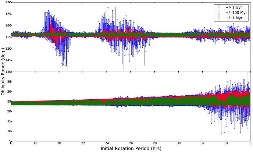
Figure 11.— Variations of hypothetical Venus’s obliquity for an initially Earth-like obliquity ($\Psi=23.45^{\circ}$) for retrograde (top panel) and prograde (bottom) rotations. The initial rotation periods are varied in 1 minute increments from 16 hr to 36 hr.

We consider the results in the context of the values for the precession constant $\alpha$ shown in Figure 1. A rapid Venus spin period of 4 hours drives a considerably large equatorial bulge (oblateness and $J_{2}$), which in turn leads to a high precession constant of 335''/yr. As this value greatly exceeds any of the frequencies of significant power in the orbital angular momentum direction power spectrum (Figure 4b), nearly all of the resulting obliquity variations remain within tight ranges ($\pm\sim 2^{\circ}$, similar to present-day Earth obliquity variability with the Moon) and non-chaotic.

At very high obliquity, however, near-resonant conditions can occur due to the $\cos{\Psi}$ dependence in Equation 2 for rotation axis precession. Hence for initial conditions with $\Psi_{0}=85^{\circ}$ and $\Psi_{0}=90^{\circ}$ we see moderately variable and chaotic obliquity variations, even for this fast 4-hour rotation period.

Retrograde rotations for the 4-hour rotation period ($\Psi>90^{\circ}$) show very low variability. Similarly small variations were seen for retrograde Moonless Earths (Lissauer et al., 2012).

Proceeding to slower rotation rates of 8, 12, and 16 hours, the low-obliquity end of the chaotic region drops to $\Psi=75^{\circ}$, $\Psi=70^{\circ}$, and $\Psi=65^{\circ}$ respectively for initial axis azimuth of $\varphi_{0}=180^{\circ}$ in Figure 7 (with similar results at $\varphi_{0}=0^{\circ}$ in Figure 6). This downward expansion of the chaotic zone is consistent with the effects of lower obliquity on precession rate from Equation 2. As the slower rotation reduces the planet’s $J_{2}$, it also diminishes its precession constant $\alpha$. Hence a lower obliquity value $\Psi$ can result in similar rotation axis precession rates as the high-obliquity 4-hour rotation case.

Importantly the slower rotation rate does not introduce new chaotic regions at lower obliquity, but rather slightly reduces the maximum obliquity at the top of the chaotic zone and substantially reduces the minimum obliquity at the bottom of the zone, leading to a wider zone overall. Hypothetical Venuses that start anywhere within the chaotic region have their obliquities vary across the entire range from the lower limit to near $90^{\circ}$ over a Gyr.

These same trends continue as we proceed down Figures 6 and 7 to longer rotational periods. From 20-hr up through 36-hr rotation periods, the overall extent of the chaotic zone at high obliquities grows. The upper limit of the primary chaotic region is always above $\Psi\sim 85^{\circ}$, but the lower boundary extends all the way down to below $\Psi=45^{\circ}$ for a 36-hour siderial rotation.

Interestingly, a new, more weakly chaotic region also appears at slower rotation rates. At 20, 24, 30, and 36 hours, some smaller initial obliquities $\Psi_{0}$ below the edge of the primary chaotic zone show moderately variable obliquities. When the initial obliquity is $\Phi_{0}=50^{\circ}$ in the 24-hour rotation case at $\varphi_{0}=180^{\circ}$ (Figure 7), for instance, the obliquity varies in the range $45^{\circ}\leq\Phi\leq 60^{\circ}$ over $\pm 1$ Gyr.

In the 30-hour and 36-hour period cases, this lower-obliquity weakly chaotic zone grows. At 36-hours, it includes all of the initial obliquities smaller than the primary zone, from $0^{\circ}\leq\Phi\leq 35^{\circ}$. Hypothetical Venuses with initial obliquities inside this weaker zone show increased obliquity variability at the $\pm\sim 15^{\circ}$ level. But with the exception of the $\Psi_{0}=10^{\circ}$, $\varphi_{0}=180^{\circ}$ case the total $\pm 1$ Gyr variability does not encompass the entire extent of the weaker chaos zone. These cases only show moderately increased obliquity variability, similar to that of Moonless Earths, which have broadly comparable nodal and axial precession rates.

Although rapidly-rotating retrograde Early Venuses lack the large-scale variations found for high prograde obliquities, in some simulations their obliquities vary much more than those of Earth would have if it lacked a large moon and rotated in the retrograde sense. In the 20-hour-rotation, $\varphi_{0}=180^{\circ}$ case, for instance (Figure 7), obliquity variations of similar magnitudes to those in the weakly chaotic low-obliquity regime appear at $\Psi_{0}=155$, $\Psi_{0}=160$, and $\Psi_{0}=165$ for instance. We did not expect to find chaotic obliquity behavior for retrograde rotations given the high degree of stability found in retrograde Moonless Earths (Lissauer et al., 2012).

4.2. Closer Look at Venus with a 20-Hour Rotation Period

4.2.1 Time-Series

Focusing on the results for Venus with a 20 hr rotation period, which show unexpected chaos for some retrograde obliquities, Figure 8 shows the full $\pm 1$ Gyr time histories for the obliquity $\Psi$ of hypothetical Venuses with initial obliquities $\Psi_{0}$ spaced out every $20^{\circ}$. The low initial obliquity cases $\Psi_{0}=0^{\circ}$, $20^{\circ}$, and $40^{\circ}$, have obliquities that vary within narrow ranges and show no chaotic long-term behavior. Similarly, the $\Psi_{0}=100^{\circ}$ and $\Psi_{0}=180^{\circ}$ cases vary uniformly within a tight band with no chaotic behavior on either the medium- or long-term.

The $\Psi_{0}=60^{\circ}$ and $80^{\circ}$ cases are within the primary chaotic region. These two cases bounce around between three smaller chaotic subregions (except for the $\Psi_{0}=80^{\circ}$ case which manages to find its way out of the chaotic region beyond 550 Myr in the past).

The retrograde $\Psi_{0}=120^{\circ}$, $\Psi_{0}=140^{\circ}$, and $\Psi_{0}=160^{\circ}$ cases display behavior qualitatively different from any seen in the Moonless Earth case, on the other hand. In these cases, our hypothetical Venus’ obliquity varies within a relatively tight $\pm 2^{\circ}$ band on both short- and medium-term timescales. On longer timescales approaching 10-100 Myr, however, the center of that tight band wanders around in obliquity $\Psi$ space up to $\pm 10^{\circ}$ (in the $\Psi_{0}=140^{\circ}$ and $\Psi_{0}=160^{\circ}$ cases; the $\Psi_{0}=120^{\circ}$ case is less adventurous).

These odd retrograde cases and the chaotic $\Psi_{0}=60^{\circ}$ and $\Psi_{0}=80^{\circ}$ situation are distinct. In the primary chaotic zone obliquity varies within a single chaotic subregion while periodically and vary rapidly traversing wide chaotic ‘bridges’ (Li & Batygin, 2014a) to neighboring chaotic subregions. These transitions between subregions last for only of order a single precession period, or $\sim 70,000$ years for hypothetical Early Venus. In contrast, the retrograde rotators with $\Psi_{0}=140^{\circ}$ and $\Psi_{0}=160^{\circ}$ continue rapid, short-term variations on $10^{5}$-year timescales. But they slowly vary in obliquity on $10^{7}$-year timescales instead of nearly instantaneous alteration of their variations into a new regime as in the primary chaotic zone.

A glance back at Figure 4 shows that the unexpected retrograde long-term variability corresponds to the locations of weak frequencies in Venus’ orbit variations. However, the power associated with those peaks is a factor of $10^{6}$ lower than the primary Solar System $s$ eigenfrequencies. Furthermore, in the 24-hour Moonless Earth case shown in Figure 5 for comparison, similar peaks in Earth’s orbital angular momentum direction frequency do not yield corresponding variability for retrograde rotators. Similarly, not all hypothetical Venuses show this behavior; retrograde rotators with 4 and 8 hour periods show little long-term obliquity variation.

4.2.2 Fine Grid in Obliquity

To further investigate this unexpected chaotic obliquity evolution in retrograde rotators, we ran additional obliquity variation integrations at very high resolution in initial obliquity $\Psi_{0}$. In this section we analyze the 20-hour-rotation-period Early Venus specifically because it shows the strongest anomalous retrograde variability. Figure 9 shows our results using a grid of 361 different $\Psi_{0}$ values spaced out every $0.5^{\circ}$. In this portion of the investigation we elect to integrate out only to $\pm 100$ Myr to allow for improved resolution in $\Psi_{0}$ within our available computing power.

We show the results of this fine $\Psi_{0}$ integration in Figure 9. We also show the analogous plot for Moonless Earths in Figure 10, seeing as Lissauer et al. (2012) did not perform such a high-resolution grid of simulations.

Similar to the coarser-gridded Lissauer et al. (2012) result, the Moonless Earth shows moderately wide $\pm\sim 10^{\circ}$ obliquity variations from $\Psi_{0}=0^{\circ}$ through $\Psi_{0}=55^{\circ}$ over $\pm 100$ Myr. More distinct chaotic subregions then extend up to $\Psi_{0}=85^{\circ}$. Even when viewed at this high resolution, though, the Moonless Earth shows no signs of anomalous behavior for retrograde rotations (although in retrospect Figure 10 from Lissauer et al. (2012) may show the incipient onset of such variations at 1 Gyr timescales).

The 20-hour hypothetical Venus in Figure 9 shows very tight obliquity ranges from $\Psi_{0}=0^{\circ}$ through $\Psi_{0}\sim 55^{\circ}$ or so, followed by the single large primary chaotic region from $\Psi_{0}=60^{\circ}$ to $\Psi_{0}=90^{\circ}$ as discussed above. The smaller chaotic subregions reveal themselves when looking at shorter 1 Myr timescales (green).

Although hypothetical 20-hour Venus shows a somewhat simpler chaotic obliquity variation structure than Moonless Earth for prograde initial conditions, the opposite is true once the planets flip over into regrograde rotation at $\Psi_{0}>90^{\circ}$. At retrograde obliquities the Moonless Earth shows minimal obliquity variations even over 100 Myr timescales.

Retrograde 20-hour Venus, on the other hand, shows broadly stable obliquities but with four modestly more variable regions centered around $\Psi_{0}=100^{\circ}$, $\Psi_{0}=120^{\circ}$, $\Psi_{0}=135^{\circ}$, and $\Psi_{0}=158^{\circ}$. These regions seem to coincide with the low-power peaks in orbital frequency space shown in Figure 4. However, we do not at present understand why these peaks are important for Venus but not for Moonless Earths, which show similar peaks in orbital frequency space.

4.2.3 Fine Grid in Rotation Period

For one last exploration of this unexpected retrograde behavior we do another set of integrations at high resolution, but this time in rotation-period space. Starting with $\Psi_{0}=23.45^{\circ}$ and $\Psi_{0}=180^{\circ}-23.45^{\circ}$, we show obliquity variations as a function of rotation rate in high resolution in Figure 11. This plot shows the obliquity variations for hypothetical Venuses over three timescales: $\pm 1$ Myr (green), $\pm 100$ Myr (red), and $\pm 1$ Gyr (blue).

For a retrograde Earth-like obliquity of $\Psi_{0}=156.55^{\circ}=180^{\circ}-23.45^{\circ}$, three independent wide-variability regions occur at rotation periods $P_{\mathrm{rot}}$ of 18.8-21 hours, 23.5-28 hours, and 31.5-36+ hours. These correspond respectively to the $r4$, $r3$, and $r2$ retrograde precession frequencies from Figure 9b. Presumably another similar region exists for even longer rotation periods corresponding to $r1$.

All told, while unexpected, these chaotic zones at retrograde rotations only show modest total variability — $\pm 7^{\circ}$ in the worst case over 1 Gyr. Understanding their origin is important for evaluating the suggestion of Lissauer et al. (2012) that “if initial planetary rotational axis orientations are isotropic, then half of all moonless extrasolar planets would be retrograde rotators, and these planets should experience obliquity stability similar to that of our own Earth, as stabilized by the presence of the Moon.” While our results show that the most variable retrograde hypothetical Venuses are more stable than the standard Moonless Earths, the same may not be true for retrograde-rotating planets in all cases.

5. Conclusions

We investigate the variations in obliquity that would be expected for hypothetical rapidly rotating Venus from early in Solar System history. These hypothetical Early Venuses allow us to investigate the conditions under which Venus’ climate may have been sufficiently stable as to allow for habitability under a faint young Sun.

Additionally, they also serve as a comparitor for potentially habitable terrestrial planets in extrasolar systems. While previous work on a moonless Earth effectively modeled a single point of comparison, the present work provides a second comparator from which we can start to imagine a more general result. These intensive, single-planet studies complement those of generalized systems (Atobe & Ida, 2007).

We show that while retrograde-rotating hypothetical Venuses show short- and medium- term obliquity stability, an unusual and as-yet-understood long-term interaction drives variability of up to $\pm 7^{\circ}$ over Gyr timescales.

The very low variability of low-obliquity hypothetical Venuses over a range of rotation rates provides additional evidence that massive moons are not necessary to mute obliquity variability on habitable worlds. We show that even in the Solar System the increased rotational axis precession rate driven by Venus’ closer proximity to the Sun is sufficient to push Venus into a benign obliquity variability regime. Indeed, Figure 4 for example indicates that for present-Earth-like initial obliquities ($\Psi_{0}=23.45^{\circ}$), the overall obliquity variability over 100 Myr for Venus with a 20-hour rotation period is similar to that for the real Earth with the Moon.

More rapid rotational axis precession will naturally result on planets in the habitable zones of lower-mass stars. While these stars’ gravity is proportionally lower, their disproportionately fainter luminosities drive the habitable zone inward from that around the present-day Sun. Thus, for similar orbital driving frequencies – i.e., a clone of the Solar System around a lower-mass star – stellar gravity alone would be sufficient to push a habitable planet’s obliquity variations into a benign regime.

Of course tides provide a drawback to using stellar proximity to speed rotational precession. In any real system, in addition to the obliquity variations that we describe here, tides will simultaneously act to upright a planet’s rotation axis and slow its rotation rate Tidal effects will be even more important on habitable zone planets around lower mass stars than they are for Earth and Venus around the Sun.

Hence a potential avenue for future work will be to couple the adiabatic obliquity variations that we describe here to tidal dissipation over time. Given that the natural variability within chaotic zones is much more rapid than tidal timescales, we suspect that the primary effect of tides will be through rotational braking. A planet with slowing rotation could traverse through various obliquity behavior regimes over its lifetime. Such a planet might then potentially have multiple possible interesting and chaotic pathways toward tidal locking, as opposed to the simpler slow obliquity reduction that would be expected in a 1-planet system.

References

- Abe et al. (2011) Abe, Y., Abe-Ouchi, A., Sleep, N. H., & Zahnle, K. J. 2011, Astrobiology, 11, 443
- Ahrens (1995) Ahrens, T. 1995, Global Earth Physics (American Geophysical Union)
- Araújo et al. (2008) Araújo, M. B., Nogués-Bravo, D., Diniz-Filho, J. A. F., et al. 2008, Ecography, 31, 8
- Armstrong et al. (2014) Armstrong, J. C., Barnes, R., Domagal-Goldman, S., et al. 2014, Astrobiology, 14, 277
- Armstrong et al. (2004) Armstrong, J. C., Leovy, C. B., & Quinn, T. 2004, Icarus, 171, 255
- Atobe & Ida (2007) Atobe, K., & Ida, S. 2007, Icarus, 188, 1
- Atobe et al. (2004) Atobe, K., Ida, S., & Ito, T. 2004, Icarus, 168, 223
- Brasser et al. (2014) Brasser, R., Ida, S., & Kokubo, E. 2014, MNRAS, 440, 3685
- Brasser & Walsh (2011) Brasser, R., & Walsh, K. J. 2011, Icarus, 213, 423
- Chambers (1999) Chambers, J. E. 1999, MNRAS, 304, 793
- Correia & Laskar (2001) Correia, A. C. M., & Laskar, J. 2001, Nature, 411, 767
- Correia & Laskar (2003) —. 2003, Icarus, 163, 24
- Correia et al. (2003) Correia, A. C. M., Laskar, J., & de Surgy, O. N. 2003, Icarus, 163, 1
- Hawkins & Porter (2003) Hawkins, B. A., & Porter, E. E. 2003, Global Ecology and Biogeography, 12, 475
- Hoffman et al. (1998) Hoffman, P. F., Kaufman, A. J., Halverson, G. P., & Schrag, D. P. 1998, Science, 281, 1342
- Hortal et al. (2011) Hortal, J., Diniz-Filho, J. A. F., Bini, L. M., et al. 2011, Ecology Letters, 14, 741
- Karttunen (2007) Karttunen, H. 2007, Fundamental astronomy (Springer Science & Business Media)
- Kurosawa (2015) Kurosawa, K. 2015, Earth and Planetary Science Letters, 429, 181
- Laskar (1996) Laskar, J. 1996, Celest. Mech. and Dyn. Astron., 64, 115
- Laskar et al. (2004) Laskar, J., Correia, A. C. M., Gastineau, M., et al. 2004, Icarus, 170, 343
- Laskar et al. (1993) Laskar, J., Joutel, F., & Robutel, P. 1993, Nature, 361, 615
- Laskar & Robutel (1993) Laskar, J., & Robutel, P. 1993, Nature, 361, 608
- Li & Batygin (2014a) Li, G., & Batygin, K. 2014a, ApJ, 790, 69
- Li & Batygin (2014b) —. 2014b, ApJ, 795, 67
- Lissauer et al. (2012) Lissauer, J. J., Barnes, J. W., & Chambers, J. E. 2012, Icarus, 217, 77
- Lucas (1980) Lucas, G. 1980, The Empire Strikes Back. Directed by Irvin Kershner; Screenplay by Leigh Brackett & Lawrance Kasdan
- Milankovič (1998) Milankovič, M. 1998, Canon of insolation and the ice-age problem (translation, Publisher: Zavod za udžbenike i nastavna sredstva)
- Morbidelli et al. (2007) Morbidelli, A., Tsiganis, K., Crida, A., Levison, H. F., & Gomes, R. 2007, AJ, 134, 1790
- Murray & Dermott (2000) Murray, C. D., & Dermott, S. F. 2000, Solar System Dynamics (New York: Cambridge University Press)
- Sackmann et al. (1993) Sackmann, I.-J., Boothroyd, A. I., & Kraemer, K. E. 1993, ApJ, 418, 457
- Spiegl et al. (2015) Spiegl, T. C., Paeth, H., & Frimmel, H. E. 2015, Earth and Planetary Science Letters, 415, 100
- Touma & Wisdom (1993) Touma, J., & Wisdom, J. 1993, Science, 259, 1294
- Touma & Wisdom (1994) —. 1994, AJ, 107, 1189