Spanners for Directed Transmission Graphs

Abstract

Let $P\subset\mathbb{R}^{2}$ be a planar $n$-point set such that each point $p\in P$ has an associated radius $r_{p}>0$. The transmission graph $G$ for $P$ is the directed graph with vertex set $P$ such that for any $p,q\in P$, there is an edge from $p$ to $q$ if and only if $d(p,q)\leq r_{p}$.

Let $t>1$ be a constant. A $t$-spanner for $G$ is a subgraph $H\subseteq G$ with vertex set $P$ so that for any two vertices $p,q\in P$, we have $d_{H}(p,q)\leq td_{G}(p,q)$, where $d_{H}$ and $d_{G}$ denote the shortest path distance in $H$ and $G$, respectively (with Euclidean edge lengths). We show how to compute a $t$-spanner for $G$ with $O(n)$ edges in $O(n(\log n+\log\Psi))$ time, where $\Psi$ is the ratio of the largest and smallest radius of a point in $P$. Using more advanced data structures, we obtain a construction that runs in $O(n\log^{5}n)$ time, independent of $\Psi$.

We give two applications for our spanners. First, we show how to use our spanner to find a BFS tree in $G$ from any given start vertex in $O(n\log n)$ time (in addition to the time it takes to build the spanner). Second, we show how to use our spanner to extend a reachability oracle to answer geometric reachability queries. In a geometric reachability query we ask whether a vertex $p$ in $G$ can “reach” a target $q$ which is an arbitrary point in the plane (rather than restricted to be another vertex $q$ of $G$ in a standard reachability query). Our spanner allows the reachability oracle to answer geometric reachability queries with an additive overhead of $O(\log n\log\Psi)$ to the query time and $O(n\log\Psi)$ to the space.

1 Introduction

A common model for wireless sensor networks is the unit-disk graph: each sensor $p$ is modeled by a unit disk centered at $p$, and there is an edge between two sensors if and only if their disks intersect [11]. Intersection graphs of disks with arbitrary radii have also been used to model sensors with different transmission strengths [4, Chapter 4]. Intersection graphs of disks are undirected. However, for some networks we may want a directed model. In such networks, a sensor $p$ that can transmit information to a sensor $q$ may not be able to receive information from $q$. This motivated various researchers to consider what we call here transmission graphs[27, 23]. A transmission graph $G$ is defined for a set $P$ of points where each point $p\in P$ has a (transmission) radius $r_{p}$ associated with it. Each vertex of $G$ corresponds to a point of $P$, and there is a directed edge from $p$ to $q$ if and only if $q$ lies in the disk $D(p)$ of radius $r_{p}$ around $p$. We weight each edge $pq$ of $G$ by the distance between $p$ and $q$, denoted by $|pq|$.

As many other kinds of geometric intersection graphs, a transmission graph may be dense and may contain $\Theta(n^{2})$ edges. Thus, if one applies a standard graph algorithm, like breadth first search (BFS), to a dense transmission graph, it runs slowly, since it requires an explicit representation of all the edges in the graph. For some applications a sparse approximation of $G$ that preserves distances suffices. Therefore, given a transmission graph $G$, implicitly represented by a list of points and their associated radii, it is desirable to construct a sparse approximation of $G$ that preserves its connectivity and proximity properties. We want to construct this approximation efficiently, without generating an explicit representation of $G$.

For any $t>1$, a subgraph $H$ of $G$ is a $t$-spanner for $G$ if the distance between any pair of vertices $p$ and $q$ in $H$ is at most $t$ times the distance between $p$ and $q$ in $G$, i.e., $d_{H}(p,q)\leq t\cdot d_{G}(p,q)$ for any pair $p,q$ (see [22] for an overview of spanners for geometric graphs). Fürer and Kasivisawnathan show how to compute a $t$-spanner for unit- and general disk graphs that are variations of the Yao graph [12, 28]. Peleg and Roditty [23] give a construction for $t$-spanners in transmission graphs in any metric space with bounded doubling dimension. We continue these studies by giving an almost linear time algorithm that constructs a $t$-spanner of a transmission graph of a planar set of points ($P\subset\mathbb{R}^{2}$) in which the edges are weighted according to the Euclidean metric (i.e. $|pq|$ is the Euclidean distance between $p$ and $q$).

Our construction is also based on the Yao graph[28]. The basic Yao graph is a $t$-spanner for the complete graph defined by $n$ points in the plane (with Euclidean distances as the weights of the edges). To determine the points adjacent to a particular point $q$, we divide the plane by equally spaced rays emanating from $q$ and connect $q$ to its closest point in each wedge (the number of wedges increases as $t$ gets smaller). Adapting this construction to transmission graphs poses a severe computational difficulty, as we want to consider, in each wedge, only the points $p$ with $q\in D(p)$ and to pick the closest point to $q$ only among those. Since finding the exact closest point turns out to be difficult, we need to relax this requirement in a subtle way, without hurting the approximation too much. This makes it possible to construct the spanner efficiently.

Even with a good $t$-spanner at hand, we sometimes wish to obtain exact solutions for certain problems on disk graphs. Working in this direction, Cabello and Jejĉiĉ gave an $O(n\log n)$ time algorithm for computing a BFS tree in a unit-disk graph, rooted at any given vertex [5]. For this, they exploited the special structure of the Delaunay triangulation of the disk centers. We show that our spanner admits similar properties for transmission graphs. As a first application of our spanner, we get an efficient algorithm to compute a BFS tree in a transmission graph rooted at any given vertex.

For another application, we consider reachability oracles. A reachability oracle is a data structure that can answer reachability queries: given two vertices $s$ and $t$ determine if there is a directed path from $s$ to $t$. The quality of a reachability oracle is measured by its query time, its space requirement, and its preprocessing time. For transmission graphs, we can ask for a more general geometric reachability query: given a vertex $s$ and any point $q\in\mathbb{R}^{2}$, determine if there is a vertex $t$ such that there is a directed path from $s$ to $t$ in $G$, and $q$ lies in the disk of $t$. We show how to extend any given reachability oracle to answer geometric queries with a small additive increase in space and query time.

Our Contribution and the Organization of the Paper.

An extended abstract of this work was presented at the 31st International Symposium on Computational Geometry [16]. This abstract also discusses the problem of constructing efficient reachability oracles for transmission graphs. While we were preparing the journal version, it turned out that a full description of our results would yield a large and unwieldy manuscript. Therefore, we decided to split our study on transmission graphs into two parts, the present paper that studies fast algorithms for spanners in transmission graphs, and a companion paper that deals with the construction of efficient reachability oracles  [17].

In Section 3, we show how to compute, for every fixed $t>1$, a $t$-spanner $H$ of $G$. Our construction is quite generic and can be adapted to several situations. In the simplest case, if the spread $\Phi$ (i.e., the ratio between the largest and the smallest distance in $P$) is bounded, we can obtain a $t$-spanner in time $O(n(\log n+\log\Phi))$ (Section 3.1). With a little more work, we can weaken the assumption to a bounded radius ratio $\Psi$ (the ratio between the largest and smallest radius in $P$), giving a running time of $O(n(\log n+\log\Psi))$ (Section 3.2). Note that a bound on $\Phi$ implies a bound on $\Psi$: let $d_{\max}$ be the largest distance and $d_{\min}$ be the smallest distance between any pair of distinct points in $P$. We can set all radii larger than $d_{\max}$ to be $d_{\max}$ and all radii smaller than $d_{\min}$ to $d_{\min}/2$. This does not change the transmission graph and we have $\Psi\leq 2\Phi$. Using even more advanced data structures, we can compute a $t$-spanner in time $O(n\log^{5}n)$, without any dependence on $\Phi$ or $\Psi$ (Section 3.3).

In Section 4.1 we show how to adapt a result by Cabello and Jejĉiĉ [5] to compute a BFS tree in a transmission graph, from any given vertex $p\in P$, in $O(n\log n)$ time, once we have the spanner ready.

In Section 4.2 we show how to use a spanner to extend a reachability oracle to answer geometric reachability queries. Specifically, we show that any reachability oracle for a transmission graph with radius ratio $\Psi$, that requires $S(n)$ space, and answers a query in $Q(n)$ time, can be extended in $O(n\log n\log\Psi)$ time, to an oracle that can answer geometric reachability queries, requires $S(n)+O(n\log\Phi)$ space, and answers a query in $Q(n)+O(\log n\log\Phi)$ time.

2 Preliminaries and Notation

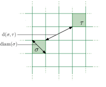
Figure 1: The grid (green) and two cells $\sigma$ and $\tau$.

We let $P\subset\mathbb{R}^{2}$ denote a set of $n$ points in the plane. Each point $p\in P$ has a radius $r_{p}>0$ associated with it. The elements in $P$ are called sites. The spread of $P$, $\Phi$, is defined as $\Phi=\max_{p,q\in P}|pq|/\min_{p\neq q\in P}|pq|$, and the radius ratio $\Psi$ of $P$ is defined as $\Psi=\max_{p,q\in P}(r_{p}/r_{q})$. A simple volume argument shows that $\Phi=\Omega(n^{1/2})$. Furthermore, as stated in the introduction, we can always assume that $\Psi\leq 2\Phi$. Given a point $p\in\mathbb{R}^{2}$ and a radius $r$, we denote by $D(p,r)$ the closed disk with center $p$ and radius $r$. If $p\in P$, we use $D(p)$ as a shorthand for $D(p,r_{p})$. We write $C(p,r)$ for the boundary circle of $D(p,r)$.

Our constructions make extensive use of planar grids. For $i\in\{0,1,\dots\}$, we define $\operatorname{\mathcal{Q}}_{i}$ to be the grid at level $i$. It consists of axis-parallel squares with diameter $2^{i}$ that partition the plane in a grid-like fashion (the cells). We write $\operatorname{diam}(\sigma)$ for the diameter of a grid cell $\sigma$. Each grid $\operatorname{\mathcal{Q}}_{i}$ is aligned so that the origin lies at the corner of a cell. The distance $d(\sigma,\tau)$ between two grid cells $\sigma,\tau$ is the smallest distance between any pair of points in $\sigma\times\tau$, see Figure 1. We assume that our model of computation allows us to find in constant time for any given point the grid cell containing it.

3 Spanners for Directed Transmission Graphs

3.1 Efficient Spanner Construction for a Set of Points with Bounded Spread

First, we give a spanner construction for the transmission graph whose running time depends on the spread. Later, in Section 3.2, we will tune this construction so that the running time depends on the radius ratio. The main result which we prove in this section is as follows.

Theorem 3.1.

Let $P$ be a set of $n$ points in the plane with spread $\Phi$. For any fixed $t>1$, we can compute, in $O(n\log\Phi)$ time, a $t$-spanner for the transmission graph $G$ of $P$. The construction needs $O(n\log\Phi)$ space.

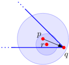
Figure 2: A cone $C_{q}$ (blue) at a site $q$. Since $q\notin D(r)$, we pick the edge $pq$.

Let $\rho$ be a ray originating from the origin and let $0<\alpha<2\pi$. A cone with opening angle $\alpha$ and middle axis $\rho$ is the closed region containing $\rho$ and bounded by the two rays obtained by rotating $\rho$ clockwise and counterclockwise by $\alpha/2$.

Given a cone $C$ and a point $q\in\mathbb{R}^{2}$, we write $C_{q}$ for the copy of $C$ obtained by translating the origin to $q$. We call $q$ the apex of $C_{q}$. Ideally, our spanner should look as follows. Let ${\mathcal{C}}$ be a set of $k$ cones with opening angles $2\pi/k$ that partition the plane. For each site $q\in P$ and each cone $C\in{\mathcal{C}}$, we pick the site $p\in P\cap C_{q}$ with $q\in D(p)$ that is closest to $q$ (see Figure 2). We add the edge $pq$ to $H$. The resulting graph has $O(kn)$ edges. Using standard techniques, one can show that $H$ is a $t$-spanner, if $k$ is large enough as a function of $t$. This construction has been reported before and seems to be folklore [7, 23].

Unfortunately, the standard algorithms for computing the Yao graph do not seem to adapt easily to our setting without a penalty in their running times [10]. The problem is that for each site $q$ and each cone $C_{q}$, we need to search for a nearest neighbor of $q$ only among those sites $p\in C_{q}$ such that $q\in D(p)$. This seems to be hard to do with the standard approaches. Thus, we modify the construction to search only for an approximate nearest neighbor of $q$ and argue that picking an approximately shortest edge in each cone suffices to obtain a spanner.

We partition each cone $C_{q}$ into “intervals” obtained by intersecting $C_{q}$ with annuli around $q$ whose inner and outer radii grow exponentially; see Figure 3. There can be only $O(\log\Phi)$ non-empty intervals. We cover each such interval by $O(1)$ grid cells whose diameter is “small” compared to the width of the interval. This gives two useful properties. (i) We only need to consider edges from the interval closest to $q$ that contains sites with outgoing edges to $q$; all other edges to $q$ will be longer. (ii) If there are multiple edges from the same grid cell, their endpoints are close together, and it suffices to consider only one of them.

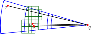
Figure 3: A cone $C_{q}$ covered by discretized intervals. We only need one of the edges $pq$, $rq$ for $H$.

To make this approach more concrete, we define a decomposition of $P$ into pairs of subsets of $P$ contained in certain grid cells. These pairs represent a discretized version of the intervals (see Definition 3.2 below). This is motivated by another spanner construction based on the well-separated pair decomposition (WSPD). Let $c>1$ be a parameter. A $c$-WSPD for $P$ is a set of pairs $(A_{i},B_{i}),\dots,(A_{m},B_{m})$ such that $A_{i},B_{i}\subseteq P$, and for each pair $a,b$ of points of $P$ there is a single index $j$ such that $a\in A_{j}$ and $b\in B_{j}$ or vice versa. Furthermore, for any $1\leq i\leq m$ we have that $c\max\{\operatorname{diam}(A_{i}),\operatorname{diam}(B_{i})\}\leq d(A_{i},B_{i})$. Here $\operatorname{diam}(A_{i})$ is the diameter of $A_{i}$ and $d(A_{i},B_{i})$ is the minimum distance between any pair $a,b$ with $a\in A_{i}$ and $b\in B_{i}$. Callahan and Kosaraju show that there always exists a WSPD with $m=O(n)$ pairs which can be computed efficiently [6].

It is well known [22] that one can obtain a $t$-spanner for the complete (undirected) Euclidean graph with vertex set $P$ from a $c$-WSPD, for a large enough $c=c(t)$, by putting in the spanner an edge $ab$ for each pair $(A_{i},B_{i})$ in the WSPD, where $a$ is an arbitrary point in $A_{i}$ and $b$ is an arbitrary point in $B_{i}$. It turns out that a similar approach works for transmission graphs. However, since they are directed, we need to find for each site in $B_{i}$ an incoming edge from a site in $A_{i}$, if such an edge exists, and vice versa. This causes two difficulties: we cannot afford to check all possible edges in $A_{i}\times B_{i}$, since this would lead to a quadratic running time, and we cannot control the indegree of a site $p$ since it may belong to many sets $A_{i}$ and $B_{i}$. We address the second problem by taking only $O(1)$ edges into a particular site $q$, within each of the $k$ cones of the Yao construction described above. For the first problem, we identify in each $A_{i}$ a special subset that “covers” all edges from a site in $A_{i}$ to a site in $B_{i}$, such that each site appears in a constant number of such subsets.

The concrete implementation of this idea is captured by Definition 3.2. A pair $(A_{i},B_{i})$ corresponds to sets $P\cap\sigma$ and $P\cap\tau$ for two grid cell $\sigma,\tau$ that have the same diameter and that are well separated (Property (i)). For a grid cell $\tau$, we denote by $m_{\tau}$ the site of largest radius in $P\cap\tau$ and we define a particular subset $R_{\tau}\subseteq P\cap\tau$ to be the set of sites assigned to $\tau$. Property (ii) in Definition 3.2 guarantees that each edge $pq$ of $G$ with $q\in\sigma$ and $p\in\tau$ is either “represented” in the decomposition by an edge originating in $m_{\tau}$ or we have that $p\in R_{\tau}$. Specifically, edges $pq$ with $q\in P\cap\sigma$ and $p\in P\cap\tau$ such that the disk $D(p)$ is “large” relative to $|pq|$ are represented by the edge $m_{\sigma}q$. This allows us to define the sets $R_{\sigma}$ such that each site appears in $O(1)$ such sets, see Figure 4.

Definition 3.2.

Let $c>2$ and let $G$ be the transmission graph of a planar point set $P$. A $c$-separated annulus decomposition for $G$ consists of a finite set $\operatorname{\mathcal{Q}}\subset\bigcup_{i=0}^{\infty}\operatorname{\mathcal{Q}}_{i}$ of grid cells, a symmetric neighborhood relation $N\subseteq\operatorname{\mathcal{Q}}\times\operatorname{\mathcal{Q}}$ between these cells, and a subset of assigned sites $R_{\sigma}\subseteq P\cap\sigma$ for each grid cell $\sigma\in\operatorname{\mathcal{Q}}$. A $c$-separated annulus decomposition for $G$ has the following properties:

1. For every $(\sigma,\tau)\in N$, $\operatorname{diam}(\sigma)=\operatorname{diam}(\tau)$, and $d(\sigma,\tau)=\gamma\operatorname{diam}(\sigma)$, for some $\gamma\in[c-2,2c)$.

2. for every edge $pq$ of $G$, there is a pair $(\sigma,\tau)\in N$ with $q\in\sigma$, $p\in\tau$, and either $p\in R_{\tau}$ or $q\in D(m_{\tau})$.

The following fact is a direct consequence of Definition 3.2. For each cell $\sigma\in\operatorname{\mathcal{Q}}$, we define its neighborhood as $N(\sigma)=\{\tau\mid(\sigma,\tau)\in N\}$.

Lemma 3.3.

For each cell $\sigma\in\operatorname{\mathcal{Q}}$, we have $|N(\sigma)|=O(c^{2})$, and for each cell $\tau\in\operatorname{\mathcal{Q}}$ the number of cells $\sigma\in\operatorname{\mathcal{Q}}$ such that $\tau\in N(\sigma)$ is $O(c^{2})$.

Proof.

This follows from Definition 3.2(i) via a standard volume argument. ∎

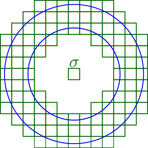
(a) By Property (i) in Definition 3.2 $N(\sigma)$ covers an annulus.

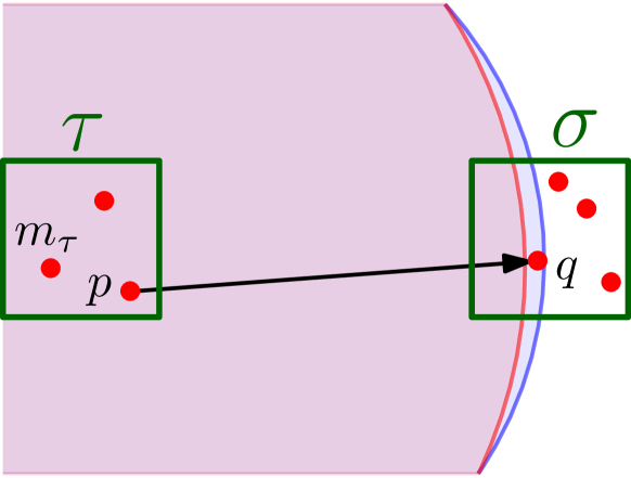
(b) Since $D(m_{\tau})$ (red) does not contain $q$, we need to put $p$ in $R_{\tau}$ to cover the edge $pq$ (Property (ii)).

Figure 4: Illustration of Definition 3.2

Given this decomposition, we first present a simple (and rather inefficient) rule for picking incoming edges such that the resulting graph is a $t$-spanner. Then we explain how to compute the decomposition using a quadtree. Finally, we exploit the quadtree to make the spanner construction efficient.

Obtaining a Spanner.

Let $t>1$ be the desired stretch. We pick a suitable separation parameter $c$ and a number of cones $k$ that depend on $t$, as specified later. Let $(\operatorname{\mathcal{Q}},N,R_{\sigma})$ be a $c$-separated annulus decomposition for $G$. For a cone $C\in{\mathcal{C}}$ and an integer $\ell\in\mathbb{N}$, we define $C^{\ell}$ as the cone with the same middle axis as $C$ but with an opening angle $\ell$ times larger than the opening angle of $C$. For $\sigma\in\operatorname{\mathcal{Q}}$, let $C_{\sigma}$ be the copy of $C$ with the center of $\sigma$ as the apex.

To obtain a $t$-spanner $H\subseteq G$, we pick the incoming edges for each site $q\in P$ and each cone $C\in{\mathcal{C}}$ as follows (see Algorithm 1). We consider the cells of $\operatorname{\mathcal{Q}}$ containing $q$ in increasing order of diameter. Let $\sigma$ be one such cell containing $q$ that we process. We traverse all neighboring cells $\tau$ of $\sigma$, that are contained in $C_{\sigma}^{2}$. For each such neighboring cell $\tau$, we check if there exists a site $r\in R_{\tau}\cup\{m_{\tau}\}$ that has an outgoing edge to $q$. If such a site exists, we add to $H$ an edge to $q$ from a single, arbitrary, such site $r$. After considering all neighbors $\tau$ of $\sigma$ we terminate the processing of $q$ and $C$ if we added at least one edge incoming to $q$. If we have not added any edge into $q$ while processing all neighbors $\tau$ of $\sigma$ we continue to the next largest cell containing $q$. We use here the extended cones $C_{\sigma}^{2}$ (instead of the cone $C_{q}$) to gain certain flexibility that will be useful for later extensions of Algorithm 1.

1 $\operatorname{\mathcal{Q}}_{q}\leftarrow$ cells of $\operatorname{\mathcal{Q}}$ that contain $q$

2 Sort the cells in $\operatorname{\mathcal{Q}}_{q}$ in increasing order by diameter

3 Make $q$ active

4 while $q$ is active do

5       $\sigma\leftarrow$ next largest cell in $\operatorname{\mathcal{Q}}_{q}$

6       foreach cell $\tau\in N(\sigma)$ that is contained in $C_{\sigma}^{2}$ do

7             if there is a $r\in R_{\tau}\cup\{m_{\tau}\}$ with $q\in D(r)$ then

8                   Take an arbitrary such $r$, add the edge $rq$ to $H$, and set $q$ to inactive

Algorithm 1 Selecting the incoming edges for $q$ and the cone $C$.

For each cone $C\in{\mathcal{C}}$ and each site $q\in P$ there is only one cell $\sigma\in\operatorname{\mathcal{Q}}_{q}$ that produces incoming edges for $q$. We have $k$ cones and $|N(\sigma)|=O(c^{2})$ by Lemma 3.3, so $q$ has $O(c^{2}k)$ incoming edges. It follows that the size of $H$ is $O(n)$ since $c$ and $k$ are constants.

Next we show that $H$ is a $t$-spanner. For this, we show that every edge $pq$ of $G$ is represented in $H$ by an approximate path. We prove this by induction on the ranks of the edge lengths. This is done in a similar manner as for the standard Yao graphs, but with a few twists that require three additional technical lemmas. Lemma 3.4 deals with the imprecision introduced by taking the cone $C_{\sigma}^{2}$ instead of $C_{q}$. It follows from this lemma that if $pq$ is contained in the cone $C_{q}$ then Algorithm 1 picks at least one edge $rq$ with $r\in C_{q}^{4}$. Lemma 3.5 and Lemma 3.6 encapsulate geometric facts that are used to bound the distance between the endpoints $r$ and $p$ depending on whether $|rq|$ is larger or smaller than $|pq|$. Lemma 3.6 is due to Bose et al. [3] and for completeness we include their proof.

Lemma 3.4.

Let $c>3+\frac{2}{\sin(\pi/k)}$ and let $\ell\in\{1,\dots,\lfloor k/2\rfloor\}$. Consider a cell $\sigma\in\operatorname{\mathcal{Q}}_{i}$ and a cone $C\in{\mathcal{C}}$. Fix two points $q,s\in\sigma$. Every cell $\tau\in\operatorname{\mathcal{Q}}_{i}$ with $d(\sigma,\tau)\geq(c-2)2^{i}$ that intersects the cone $C^{\ell}_{q}$ is contained in the cone $C_{s}^{2\ell}$. In particular, any point $p\in C_{q}^{\ell}$ with $|pq|\geq(c-2)2^{i}$ lies in a cell that is fully contained in $C_{s}^{2\ell}$.

Proof.

Let $x$ be a point in $\tau\cap C^{\ell}_{q}$. By assumption, $|xq|\geq(c-2)2^{i}$. Let $D=D(x,2^{i})$ be the disk with center $x$ and radius $2^{i}$. Then, $\tau\subseteq D$. We show that $C_{s}^{2\ell}$ contains $D$ and thus $\tau$. Since $\sigma$ has diameter $2^{i}$, and $C_{q}^{\ell}$ contains $x$, the translated copy $C_{s}^{\ell}$ must intersect $D$. If $D\subset C_{s}^{\ell}$, we are done. Otherwise, there is a boundary ray $\rho$ of $C_{s}^{\ell}$ that intersects the boundary of $D$. Let $y$ be the first intersection of $\rho$ with the boundary of $D$. See Figure 5.

Since $s\in\sigma$ and $x\in\tau$, the triangle inequality gives that $|ys|\geq|xs|-|xy|\geq(c-3)2^{i}$. Let $\rho^{\prime}$ be the boundary ray of $C_{s}^{2\ell}$ corresponding to $\rho$ and let $y^{\prime}$ be the orthogonal projection of $y$ onto $\rho^{\prime}$. Since $|ys|\geq(c-3)2^{i}$ and since the angle between $\rho$ and $\rho^{\prime}$ is $\pi\ell/k$, we get that $|yy^{\prime}|\geq(c-3)2^{i}\sin(\pi\ell/k)$. It follows that $|yy^{\prime}|\geq 2\cdot 2^{i}$ for $c>3+\frac{2}{\sin(\pi\ell/k)}$. This holds for any $\ell\in\{1,\dots,\lfloor k/2\rfloor\}$ if $c\geq 3+\frac{2}{\sin(\pi/k)}$. Thus, $\tau\subset D\subset C_{s}^{2\ell}$. ∎

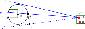
Figure 5: The boundary ray $\rho$ of $C_{s}^{\ell}$ intersects the boundary of $D$ in $y$.

Let $p$ be a site in $C_{q}$ such that $pq$ is an edge of $G$, and $p\in\tau\in N(\sigma)$ where $\sigma$ is a cell containing $q$. Then by Lemma 3.4, $\tau$ is contained in $C_{\sigma}^{2}$. It follows that Algorithm 1 either finds an edge $rq$ before processing $\sigma$, or finds an edge $rq$ with $r\in\tau$ while processing $\sigma$. By applying Lemma 3.4 again we get that $r\in C_{q}^{4}$. This fact is described in greater detail and is being used in the proof of Lemma 3.7 below.

Lemma 3.5.

Let $C\in{\mathcal{C}}$, and let $q\in\mathbb{R}^{2}$. Suppose there are two points $p,r\in C_{q}^{4}$ with $(c-2)2^{i}\leq|pq|\leq|rq|\leq(c+1)2^{i}$. Then $|pr|\leq((8\pi/k)(c+1)+3)2^{i}$.

Proof.

The points $p$ and $r$ lie in an annulus around $q$ with inner radius $(c-2)2^{i}$ and outer radius $(c+1)2^{i}$. Since $p,r\in C_{q}^{4}$, when going from $p$ to $r$, we must travel at most $(8\pi/k)(c+1)2^{i}$ units along the circle around $q$ with $p$ on the boundary, then at most $3\cdot 2^{i}$ units radially towards $r$. Thus, $|pr|\leq(8\pi/k)(c+1)2^{i}+3\cdot 2^{i}$. ∎

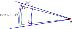
(a) Lemma 3.5. Two sites in an annulus are close to each other.

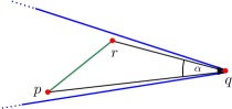
(b) Lemma 3.6. If $\alpha$ is small and $|rq|\leq|pq|$, then $|pr|<|pq|$.

Lemma 3.6 (Lemma 10 in [3]).

Let $k\geq 25$ be large enough such that

$$\frac{1+\sqrt{2-2\cos(8\pi/k)}}{2\cos(8\pi/k)-1}=1+\Theta(1/k)\leq t$$

for our desired stretch factor $t$. For any three distinct points $p,q,r\in\mathbb{R}^{2}$ such that $|rq|\leq|pq|$ and $\alpha=\angle pqr$ is between $0$ and $8\pi/k$, we have $|pr|\leq|pq|-|rq|/t$.

Proof.

By the law of cosines and since $0\leq\alpha\leq 8k/\pi$ we have that

$$|pr|^{2} =|pq|^{2}+|rq|^{2}-2|pq|\cdot|rq|\cos\alpha\leq|pq|^{2}+|rq|^{2}-2|pq|\cdot|rq|\cos(8\pi/k)$$

Introducing $$t$$ by adding and subtracting equal terms, this is

$$=|pq|^{2}-\frac{2}{t}\,|pq|\cdot|rq|+\frac{1}{t^{2}}|rq|^{2}+\frac{t^{2}-1}{t^{2}}|rq|^{2}-\frac{2(t\cos(8\pi/k)-1)}{t}|pq|\cdot|rq|$$

$$=\Bigl{(}|pq|-\frac{|rq|}{t}\Bigr{)}^{2}+\frac{t^{2}-1}{t^{2}}|rq|^{2}-\frac{2(t\cos(8\pi/k)-1)}{t}|pq|\cdot|rq|.$$

We complete the proof by showing that under the assumptions of the lemma $\frac{t^{2}-1}{t^{2}}|rq|^{2}-\frac{2(t\cos(8\pi/k)-1)}{t}|pq|\cdot|rq|\leq 0$. We have that

$$\frac{t^{2}-1}{t^{2}}|rq|^{2}-\frac{2(t\cos(8\pi/k)-1)}{t}|pq|\cdot|rq| =\frac{|rq|^{2}}{t^{2}}\Bigl{(}t^{2}-1-2(t^{2}\cos(8\pi/k)-t)\frac{|pq|}{|rq|}\Bigr{)}$$

$$\leq\frac{|rq|^{2}}{t^{2}}\Bigl{(}t^{2}-1-2(t^{2}\cos(8\pi/k)-t)\Bigr{)},$$

where the last inequality follows since $|pq|\geq|rq|$ and

$$t\geq\frac{1+\sqrt{2-2\cos(8\pi/k)}}{2\cos(8\pi/k)-1}\geq\frac{1}{2\cos(8\pi/k)-1}\geq\frac{1}{\cos(8\pi/k)}\ ,$$

so $t\cos(8\pi/k)\geq 1$. Now we have that

$$t^{2}-1-2(t^{2}\cos(8\pi/k)-t)=(1-2\cos(8\pi/k))t^{2}+2t-1\leq 0$$

if $\cos(8\pi/k)>1/2$ and

$$\frac{1+\sqrt{2-2\cos(8\pi/k)}}{2\cos(8\pi/k)-1}\leq t\ .$$

The latter inequality holds by assumption and $\cos(8\pi/k)>1/2$ for $k\geq 25$. ∎

We are now ready to bound the stretch of the spanner $H$. This is done in two steps. In the first step (Lemma 3.7) we prove that for any edge $pq$ of $G$ which is not in $H$, there exists a shorter edge $rq$ in $H$, such that $r$ is “close” to $p$. This fact allows us to prove, via a fairly standard inductive argument, that $H$ is indeed a spanner of $G$.

Lemma 3.7.

Let $c$ and $k$ be such that $c>3+\frac{2}{\sin(\pi/k)}$ as required by Lemma 3.4, $k$ satisfies the conditions of Lemma 3.6 and, in addition, $c\geq 2+\frac{2t}{t-1}$ and $k\geq\frac{16\pi t}{t-1}$. Let $pq$ be an edge of $G$. Then either $pq$ is in $H$ or there is an edge $rq$ in $H$ such that $|pr|\leq|pq|-|rq|/t$.

Proof.

Let $N$ be the neighborhood relation of the $c$-separated annulus decomposition used by Algorithm 1. Let $(\sigma,\tau)\in N$ be a pair of neighboring cells satisfying requirement (ii) of Definition 3.2 with respect to $pq$. In particular we have that $q\in\sigma$ and $p\in\tau$. If there is more than one such pair $(\sigma,\tau)\in N$, we consider the pair with minimum diameter. Let $\operatorname{diam}(\sigma)=2^{i}$, that is $\sigma,\tau\in\operatorname{\mathcal{Q}}_{i}$.

Let $C\in{\mathcal{C}}$ be the cone such that $p\in C_{q}$. Since $p\in C_{q}\cap\tau$ and since $d(\sigma,\tau)\geq(c-2)2^{i}$, Lemma 3.4 implies that $\tau\subset C_{\sigma}^{2}$. Hence, $\tau$ is considered for incoming edges for $q$ (line 1 in Algorithm 1). We split the rest of the proof into two cases.

Case 1: $q$ remains active until $(\sigma,\tau)$ is considered. Requirement (ii) of Definition 3.2 guarantees that Algorithm 1 finds an incoming edge $rq$ for $q$ with $r\in\tau$. If $r=p$, we are done, so suppose that $r\neq p$. Since $\operatorname{diam}(\sigma)=2^{i}$ and $|rq|\geq d(\sigma,\tau)\geq(c-2)2^{i}$ we have

$$|pr| \leq 2^{i}=|pq|-(|pq|-2^{i})\leq|pq|-(|rq|-2\cdot 2^{i})$$

$$\leq|pq|-(|rq|-2|rq|/(c-2))\leq|pq|-|rq|(1-2/(c-2))\leq|pq|-|rq|/t,$$

for $c\geq 2+\frac{2t}{t-1}$.

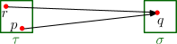
(a) Case 1: $p$ and $r$ are in the same cell $\sigma$.

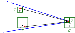
(b) Case 2: $p$ and $r$ are in different cells with different levels but in the same cone $C_{q}^{4}$.

Case 2: $q$ becomes inactive before $(\sigma,\tau)$ is considered. Then Algorithm 1 has selected an edge $rq$ while considering a pair $(\bar{\sigma},\bar{\tau})\in N$ with $q\in\bar{\sigma}$, $r\in\bar{\tau}$ and $\operatorname{diam}(\bar{\sigma})\leq 2^{i-1}$. We now distinguish two subcases.

Subcase 2a $|rq|\geq|pq|$. From Property (i) of Definition 3.2, it follows that $d(\sigma,\tau)\geq(c-2)2^{i}$ and therefore $|pq|\geq(c-2)2^{i}$. It also follows from the same property that $d(\bar{\sigma},\bar{\tau})\leq 2c2^{i-1}$, so $|rq|\leq 2c2^{i-1}+2\cdot 2^{i-1}=(c+1)2^{i}$. Combining these inequalities we obtain that $(c-2)2^{i}\leq|pq|\leq|rq|\leq(c+1)2^{i}$ and therefore $|pq|\geq|rq|-3\cdot 2^{i}$. Lemma 3.5 implies that $|pr|\leq((8\pi/k)(c+1)+3)2^{i}$, and thus we have

$$|pr| \leq((8\pi/k)(c+1)+3)2^{i}$$

$$\leq|pq|-|pq|+((8\pi/k)(c+1)+3)2^{i}$$

$$\leq|pq|-\bigl{(}|rq|-3\cdot 2^{i}-((8\pi/k)(c+1)+3)2^{i}\bigr{)}$$

$$\leq|pq|-\Bigl{(}|rq|-\frac{(8\pi(c+1)-6)2^{i}}{k}\Bigr{)}$$

$$\leq|pq|-|rq|\Bigl{(}1-\frac{(8\pi(c+1)-6)}{k(c-2)}\Bigr{)}$$

$$\leq|pq|-|rq|\Bigl{(}1-\frac{16\pi}{k}\Bigr{)}\ .$$

The third inequality follows since $|pq|\geq|rq|-3\cdot 2^{i}$ as we argued above, and the fifth inequality follows since $2^{i}\leq|rq|/(c-2)$. The last inequality holds for $c\geq 5$ (which follows from our assumptions). Now we clearly have that

$$|pq|-|rq|\Bigl{(}1-\frac{16\pi}{k}\Bigr{)}\leq|pq|-|rq|/t,$$

for $k\geq\frac{16\pi t}{t-1}$.

Subcase 2b $|rq|<|pq|$. By assumption, we have $p\in C_{q}\subset C_{q}^{4}$. Furthermore, by applying Lemma 3.4 with the midpoint of $\bar{\sigma}$ as $q$, $r$ as $p$, and $q$ as $s$, in the statement of the lemma, we get that $r\in C_{q}^{4}$. Since $p,r\in C_{q}^{4}$ and since the opening angle of $C_{q}^{4}$ is $8\pi/k$, it follows from Lemma 3.6 that $|pr|\leq|pq|-|rq|/t$. ∎

Lemma 3.8.

For any $t>1$, there are constants $c$ and $k$ such that $H$ is a $t$-spanner for the transmission graph $G$.

Proof.

We pick the constants $c$ and $k$ so that Lemma 3.7 holds. We prove by induction on the indices of edges when ordered by their lengths, that for each edge $pq$ of $G$, there is a path from $p$ to $q$ in $H$ of length at most $t|pq|$. For the base case, consider the shortest edge $pq$ in $G$. By Lemma 3.7, if $pq$ is not in $H$ then there is an edge $rq$ in $H$ such that $|pr|\leq|pq|-|rq|/t$. Since $pq$ is an edge of $G$, it follows that $r_{p}\geq|pq|$ and therefore $pr$ must also be an edge of $G$, and it is shorter than $pq$. This gives a contradiction and therefore $pq$ must be in $H$.

For the induction step, consider an edge $pq$ of $G$. If $pq$ is in $H$ we are done. Otherwise by Lemma 3.7 there is an edge $rq$ in $H$ such that $|pr|\leq|pq|-|rq|/t$. As argued above, $pr$ is an edge of $G$ shorter than $|pq|$ so by the induction hypothesis, there is a path from $p$ to $r$ in $H$ of length no larger than $t|pr|$. It follows that

$$d_{H}(p,q)\leq d_{H}(p,r)+|rq|\leq t|pr|+|rq|\leq t(|pq|-|rq|/t)+|rq|\leq t|pq|,$$

as required. ∎

Finding the Decomposition.

We use a quadtree to define the cells of the decomposition. We recall that a quadtree is a rooted tree $T$ in which each internal node has degree four. Each node $v$ of $T$ is associated with a cell $\sigma_{v}$ of some grid $\operatorname{\mathcal{Q}}_{i}$, $i\geq 0$, and if $v$ is an internal node, the cells associated with its children partition $\sigma_{v}$ into four congruent squares, each with diameter $\operatorname{diam}(\sigma_{v})/2$. If $\sigma_{v}$ is from $\operatorname{\mathcal{Q}}_{i}$ then we say that $v$ is of level $i$. Note that all nodes of $T$ at the same distance from the root are of the same level.

Let $c$ be the required parameter for the annulus decomposition. We scale $P$ such that the closest pair in $P$ has distance $c$. (We use $P$ to denote also the scaled point set). Let $L$ be the smallest integer such that we can translate $P$ so that it fits in a single cell $\sigma$ of $\operatorname{\mathcal{Q}}_{L}$. Since $c$ is constant and $P$ has spread $\Phi$, the diameter of $P$ (after scaling) is $c\Phi$ and therefore $L=O(\log\Phi)$. We translate $P$ so that it fits in $\sigma$ and we associate the root $r$ of our quadtree $T$ with this cell $\sigma$, i.e.  $\sigma_{r}=\sigma$. By the definition of a level, $r$ is of level $L$.

We continue constructing $T$ top down as follows. We construct level $i-1$ of $T$, given level $i$, by splitting the cell $\sigma_{v}$ of each node $v$, whose cell $\sigma_{v}$ is not empty, into four congruent squares, and associate each of these squares with a child of $v$. We stop the construction of $T$ after generating the cells of level $0$. The scaling which we did to $P$ ensures that each cell of a leaf node at level $0$ contains at most one site.

We now set $\operatorname{\mathcal{Q}}=\{\sigma_{v}\mid v\in T\}$. We define $N$ as the set of all pairs $(\sigma_{v},\sigma_{w})\in\operatorname{\mathcal{Q}}\times\operatorname{\mathcal{Q}}$ such that $v$ and $w$ are at the same level in $T$ and $d(\sigma_{v},\sigma_{w})\in[c-2,2c)\operatorname{diam}(\sigma_{v})$. For $\sigma\in\operatorname{\mathcal{Q}}$, we define $R_{\sigma}$ to be the set of all sites $p\in\sigma\cap P$ with $r_{p}\in[c,2(c+1))\operatorname{diam}(\sigma_{v})$.

Lemma 3.9.

$(\operatorname{\mathcal{Q}},N,R_{\sigma})$ is a $c$-separated annulus decomposition for $G$.

Proof.

Property (i) of Definition 3.2 follows by construction. To prove that Property (ii) holds consider an edge $pq$ of $G$. Let $i$ be the integer such that $|pq|\in[c,2c)2^{i}$. Let $\sigma,\tau$ be the cells of $\operatorname{\mathcal{Q}}_{i}$ with $p\in\sigma$ and $q\in\tau$. By construction, $\sigma$ and $\tau$ are assigned to nodes of the quadtree and thus contained in $\operatorname{\mathcal{Q}}$. Since $\operatorname{diam}(\sigma)=\operatorname{diam}(\tau)=2^{i}$, we have

$$(c-2)2^{i}\leq|pq|-2\operatorname{diam}(\sigma)\leq d(\sigma,\tau)\leq|pq|<c2^{i+1},$$

and therefore $(\sigma,\tau)\in N$ by our definition of $N$. Since $pq$ is an edge of $G$, it follows that $r_{p}\geq|pq|\geq c2^{i}$. If $r_{p}<(c+1)2^{i+1}$, then $p\in R_{\sigma}$. Otherwise, $r_{m_{\sigma}}\geq r_{p}\geq(c+1)2^{i+1}$, and $q\in\tau\subset D(m_{\sigma})$. ∎

Computing the Edges of $H$.

We find edges for each cone $C\in{\mathcal{C}}$ separately as follows. For each pair of neighboring cells $\sigma$ and $\tau\in N(\sigma)$ such that $\tau$ is contained in $C_{\sigma}^{2}$ we find all incoming edges to sites in $\sigma$ from sites in $\tau$ simultaneously. To do this efficiently, we need to sort the sites in $\sigma$ along the $x$ and $y$ directions. Therefore, we process the cells bottom-up along $T$ in order of increasing levels. This way we can obtain a sorted list of the sites in each cell $\sigma$ by merging the sorted lists of its children. See Algorithm 2.

1 for $i=0,\dots,L$ do

2       foreach $v\in T$ of level $i$ do

3             $Q\leftarrow$ active sites in $\sigma_{v}\cap P$

             // preproccesing

4             Sort $Q$ in $x$ and $y$-direction by merging the sorted lists of the children of $v$ foreach $\tau\in N(\sigma_{v})$ contained in $C_{\sigma_{v}}^{2}$ do

5                   $R\leftarrow R_{\tau}\cup\{m_{\tau}\}$

                   // edge selection

6                   For each site $q\in Q$, find a $r\in R$ with $q\in D(r)$, if it exists; add the edge $rq$ to $H$

7                  

8            Set all $q\in Q$ for which at least one incoming edge was found to inactive

Algorithm 2 Selecting the edges for $H$ for a fixed cone $C$.

Note that the edges selected by Algorithm 2 have the same properties as the edges selected by Algorithm 1. Thus, by Lemma 3.8, the resulting graph is a $t$-spanner. Let $Q$ be the set of active sites in $\sigma_{v}$ when processing $v$. Let $\tau\in N(\sigma_{v})$ such that $\tau$ is contained in $C_{\sigma_{v}}^{2}$ and let $R=R_{\tau}\cup\{m_{\tau}\}$. Assume $|Q|=n$ and $|R|=m$. To find the edges from sites in $R$ to sites in $Q$ efficiently, we use the fact that these sets of sites are separated by a line parallel to either the $x$- or the $y$-axis.

Assume without loss of generality that $\ell$ is the $x$-axis, the sites of $R$ are above $\ell$ and the sites of $Q$ are below $\ell$, and assume that $Q$ is sorted along $\ell$. For each site $p\in R$ we take the part of $D(p)$ which lies below $\ell$ and compute the union of these “caps”. This union is bounded from above by $\ell$ and from below by the lower envelope of the arcs of the boundaries of the caps. The complexity of the boundary of this union is $O(m)$ and it can be computed in $O(m\log m)$ time [25]. See Figure 8.

Once we have computed this union we check for each $q\in Q$ whether $q$ lies inside it. This can be done by checking whether the intersection, $z$, of a vertical line through $q$ with the union is above or below $q$. If $q$ is above $z$ then we add the edge $rq$ to $H$ where $r$ is the site such that $z\in{\partial}D(r)$. We perform this computation for all sites in $Q$ together by a simple sweep in the $x$-direction while traversing in parallel the lower envelope of the caps and the sites of $Q$. This clearly takes $O(m+n)$ time.

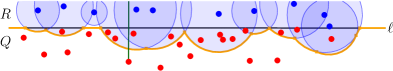
Figure 8: The lower envelope (orange), the sites $Q$ (red) and $R$ (blue), and the sweepline (green).

We thus proved the following lemma.

Lemma 3.10.

Let $Q$, $R$, and $\ell$ be as above with $|Q|=n$ and $|R|=m$. Suppose that $Q$ is sorted along $\ell$ and that $\ell$ separates $Q$ and $R$. We can compute in $O(m\log m+n)$ time for each $q\in Q$ one disk from $R$ that contains it, provided that such a disk exists.

Analysis.

We prove that Algorithm 2 runs in $O(n\log\Phi)$ time and uses $O(n\log\Phi)$ space. The running time is dominated by the edge selection step described in Lemma 3.10. We argue that each site participates in $O(1)$ edge selection steps as a disk center (in $R$) and in $O(\log\Phi)$ edge selection steps as a vertex looking for incoming edges. From these observations (and the fact that $\Phi=\Omega(n^{1/2})$) the stated time bound essentially follows.

Lemma 3.11.

We construct the spanner $H$ of the transmission graph $G$ in $O(n\log\Phi)$ time and space.

Proof.

The quadtree $T$ can be computed in $O(n\log\Phi)$ time and space [2], and within this time bound we can also compute $N(\sigma_{v})$, $R_{\sigma_{v}}$, and $m_{\sigma_{v}}$ for each node $v\in T$.

Merging the sorted lists of the sites in $\sigma_{w}$ for each child $w$ of $v$ to obtain the sorted list of the sites in $\sigma_{v}$ (line 2 in Algorithm 2) takes time linear in the number of sites in $\sigma_{v}$. Summing up over all nodes $v$ in a single level of $T$ we get that the total merging time per level is $O(n)$, and $O(n\log\Phi)$ for all levels.

To analyze the time taken by the edge selection steps (line 2 in Algorithm 2), consider a particular pair $(\sigma,\tau)\in N$ for which the algorithm runs the edge selection step. By Lemma 3.10, if we charge $m_{\tau}$ by $O(1)$, each disk center in $R_{\tau}$ by $O(\log n)$ and each active site in $\sigma\cap P$ by $O(1)$ then the total charges cover the cost of the edge selection step for $(\sigma,\tau)$. There are $O(n\log\Phi)$ nodes in $T$ and therefore $O(n\log\Phi)$ cells $\tau$ in $\operatorname{\mathcal{Q}}$. By Lemma 3.3 each such cell $\tau$ participates in an edge selection step of $O(c^{2})=O(1)$ pairs. So the total charges to the site $m_{\tau}$ over all cells $\tau$, is $O(n\log\Phi)$.

By construction, each $p\in P$ is assigned to $O(1)$ sets $R_{\tau}$ and by Lemma 3.3 each $\tau$ participates in an edge selection steps of $O(c^{2})=O(1)$ pairs. It follows that the total charges to a site $p$ from edge selections steps of pairs $(\sigma,\tau)$ such that $p\in R_{\tau}$ is $O(\log n)$.

Finally, each site is active for $O(c^{2})=O(1)$ pairs in $N$ at each of $O(\log\Phi)$ levels. So the total charges to a site $p$ from edge selections steps of pairs $(\sigma,\tau)$ such that $p$ is active in $\sigma\cap P$ is $O(n\log\Phi)$. We conclude that the total running time of all edge selection steps is $O(n\log n+n\log\Phi)=O(n\log\Phi)$, since $\log\Phi=\Omega(\log n)$. ∎

Theorem 3.1 follows by combining Lemmas 3.8 and 3.11.

3.2 From Bounded Spread to Bounded Radius Ratio

Let $P\subset\mathbb{R}^{2}$ be a set of sites with radius ratio $\Psi$. We extend our spanner construction from Section 3.1 such that the running time depends on $\Psi$, the ratio between the largest to smallest radii, rather than on the spread $\Phi$. This is a more general result as we may assume that $\Psi\leq 2\Phi$ (see Section 2). We prove the following theorem.

Theorem 3.12.

Let $P$ be a set of $n$ sites in the plane with radius ratio $\Psi$. For any fixed $t>1$, we can compute a $t$-spanner for the transmission graph $G$ of $P$ in $O(n(\log n+\log\Psi))$ time and $O(n\log\Psi)$ space.

The main observation which we use is that sites that are close together form a clique in $G$ and can be handled using classic spanner constructions, while sites that are far away from each other belong to distinct components of $G$ and can be dealt with independently.

Given $t$, we pick sufficiently large constants $k=k(t)$ and $c=c(t)$ as specified in Section 3.1. We scale the input such that the smallest radius is $c$. Let $M=c\Psi$ be the largest radius after we did the scaling. First, we partition $P$ into sets that are far apart and can be handled separately.

Lemma 3.13.

We can partition $P$ into sets $P_{1},\dots,P_{\ell}$, such that each set $P_{i}$ has diameter $O(n\Psi)$ and for any $i\neq j$, no site of $P_{i}$ can reach a site of $P_{j}$ in $G$. Computing the partition takes $O(n\log n)$ time and $O(n)$ space.

Proof.

We assign to each site $p\in P$ an axis-parallel square $S_{p}$ that is centered at $p$ and has side-length $2M$. We define the intersection graph $G_{S}$ that has a vertex for each site in $P$, and an edge between two vertices $p$ and $q$ if and only if $S_{p}\cap S_{q}\neq\emptyset$. ($G_{S}$ is undirected.)

If follows that if there is no (undirected) path from $p$ to $q$ in $G_{S}$, then there is no (directed) path from $p$ to $q$ in $G$. We can compute the connected components of $G_{S}$ in $O(n\log n)$ time by sweeping the plane using a binary search tree [24]. Let $P_{1},\dots,P_{\ell}$ be the vertex sets of these connected components. By construction, each set of sites $P_{i}$ has diameter $O(nM)$ and for any $i\neq j$, no site in $P_{i}$ can reach a site in $P_{j}$ in $G$. ∎

By Lemma 3.13, we may assume that the diameter of our input set $P$ is $O(n\Psi)$. We compute a hierarchical decomposition $T$ for $P$ as in Section 3.1, with a little twist as follows. We translate $P$ so that it fits in a single grid cell $\sigma$ of diameter $O(n\Psi)$. Starting from $\sigma$, we recursively subdivide each non-empty cell into four congruent cells of half the diameter. We do not subdivide cells of level $0$ whose diameter is $1$. We partition all cells of a particular level in $O(n)$ time and $O(n)$ space.

We construct a quadforest $T$ such that the roots of its trees correspond to the non-empty cells of level $L=\lceil\log\Psi\rceil$ in our decomposition. Each internal node of $T$ corresponds to a non-empty cell obtained when subdividing the cell of its parent. It suffices to store only the lowest $L$ levels, since larger cells cannot contribute any edges to the spanner (as we will argue below). The forest $T$ requires $O(n\log\Psi)$ space and we compute it in $O(n(\log n+\log\Psi))$ time.

We cannot derive from $T$ a $c$-separated annulus decomposition for $G$ as we did in Section 3.1. In particular a cell corresponding to a leaf of $T$ may now contain many sites that are adjacent in $G$. For edges induced by such pairs of sites we cannot satisfy Property (ii) of Definition 3.2.

We can (and do) derive from $T$ a partial $c$-separated annulus decomposition $(\operatorname{\mathcal{Q}},N,R_{\sigma})$ exactly as described in Section 3.1 before Lemma 3.9. This decomposition satisfies Property (ii) of Definition 3.2 for all edges $pq$ with $d(\sigma,\tau)\geq(c-2)$, where $\sigma$ and $\tau$ are the level 0 cells of $T$ containing $q$ and $p$, respectively. The proof that Property (ii) of Definition 3.2 holds for these edges is the same as the proof of Lemma 3.9. In particular, in the proof of Lemma 3.9, we argue that pairs of cells at level $i$ guarantee Property (ii) of Definition 3.2 for edges of length in $[c,2c)2^{i}$. Since the edges of $G$ are of length at most $M=c\Psi$, the cells up to level $L=\lceil\log\Psi\rceil$ suffice to guarantee Property (ii) of Definition 3.2 for all edges $pq$ with $d(\sigma,\tau)\geq(c-2)$.

We mark all sites of $P$ as active, and we run Algorithm 2 of Section 3.1 using $T$ and the partial $c$-separated annulus decomposition that we derived from it. The resulting graph $H$ is not yet a $t$-spanner since the decomposition was only partial.

To make $H$ a spanner we add to it more edges that “take care” of the edges not “covered” by the $c$-separated annulus decomposition. We consider each pair of level $0$ cells $\sigma$ and $\tau$ with $d(\sigma,\tau)<c-2$. The set of sites $Q=(P\cap\sigma)\cup(P\cap\tau)$ form a clique, since the distance between each pair of sites in $Q$ is no larger than $c$. We compute a Euclidean $t$-spanner for $Q$ of size $O(|Q|)$ in $O(|Q|\log|Q|)$ time [22] and for each (undirected) edge $pq$ of this spanner we add $pq$ and $qp$ to $H$. As each site $p\in P$ participates in $O(c^{2})$ such spanners, we generate in total $O(n)$ edges in $O(n\log n)$ time.

We now prove that $H$ is indeed a $t$-spanner. The proof is analogous to the proof of Lemma 3.8.

Lemma 3.14.

For any $t>1$, there are constants $c=c(t)$ and $k=k(t)$ such that $H$ is a $t$-spanner for the transmission graph $G$.

Proof.

By construction, $H$ is a subgraph of $G$. Let $pq$ be an edge of $G$, and let $\sigma$ and $\tau$ be the level $0$ cells with $q\in\sigma$ and $p\in\tau$. If $d(\sigma,\tau)<c-2$, then the Euclidean $t$-spanner for $\sigma$ and $\tau$ contains a path from $p$ to $q$ of length at most $t|pq|$.

For the remaining edges, the lemma is proved by induction on the rank of the edges when we sort them by length, as in Lemma 3.8. The proof is almost verbatim as before; we only comment on the base case. Let $pq$ be the shortest edge in $G$. If the endpoints $p$ and $q$ lie in level 0 cells whose distance is less than $c-2$, we have already argued that $H$ contains an approximate path from $p$ to $q$. Otherwise, the same argument as in Lemma 3.8 applies, and the algorithm includes $pq$ in $H$. ∎

Using Lemma 3.14, Theorem 3.12 follows just as Theorem 3.1 in Section 3.1. The analysis of the space and time required by our construction is exactly as in Lemma 3.11, but now $T$ has $O(\log\Psi)$ levels.

3.3 Spanners for Unbounded Spread and Radius Ratio

We eliminate the dependency of our bounds on the radius ratio at the expense of a more involved data structure and an additional polylogarithmic factor in the running time. Given $P\subset\mathbb{R}^{2}$ and the desired stretch factor $t>1$, we choose appropriate parameters $c=c(t)$ and $k(t)$ as in Section 3.2 and rescale $P$ such that the distance between the closest pair of points in $P$ is $c+2$.

To get the spanner of $G$ we compute a compressed quadtree $T$ for $P$. A compressed quadtree is a rooted tree in which each internal node has degree $1$ or $4$. Each node $v$ is associated with a cell $\sigma_{v}$ of a grid $\operatorname{\mathcal{Q}}_{i}$. If $v$ has degree $4$, then the cells associated of its children partition $\sigma_{v}$ into $4$ congruent squares of half the diameter, and at least two of them must be non-empty. If $v$ has degree $1$, then the cell associated with the only child $w$ of $v$ has diameter at most $\operatorname{diam}(v)/4$ and $(\sigma_{v}\setminus\sigma_{w})\cap P=\emptyset$. Each internal node of $T$ contains at least two sites in its cell and each leaf at most one site. For technical reasons we assume that the cell associated with a leaf $v$ has diameter $1$. Since $v$ contains a single point $p$ we can artificially guarantee this by shrinking the cell associated with $v$ to the cell of diameter one containing $p$.

Note that, in contrast with (uncompressed) quadtrees, the diameter of $\sigma_{v}$ may be smaller than $2^{L-i}$, where $i$ is the the distance of $v$ to the root and $2^{L}$ is the diameter of the root. A compressed quadtree for $P$ with $O(n)$ nodes can be computed in $O(n\log n)$ time [13].

To simplify the notation in the rest of this section, we write $\operatorname{diam}(v)$ instead of $\operatorname{diam}(\sigma_{v})$, and for two nodes $v,w$, we write $d(v,w)$ for $d(\sigma_{v},\sigma_{w})$.

Our approach is to use the algorithm from Section 3.1 on the compressed quadtree $T$. One problem with this approach is that the depth of $T$ may be linear, so considering all sites for incoming edges at each level, as in Algorithm 2, would be too expensive. We tackle this difficulty by using Chan’s dynamic nearest neighbor data structure to speed up this stage. We achieve this speedup by reusing at a node $v$ the largest structure among the structures at the children of $v$. The data structure of Chan has the following properties.

Theorem 3.15 (Chan, Afshani and Chan, Chan and Tsakalidis, Kaplan et al [1, 8, 9, 18]).

There exists a dynamic data structure that maintains a planar point set $S$ such that

1. we can insert a point into $S$ in $O(\log^{3}n)$ amortized time;

2. we can delete a point from $S$ in $O(\log^{5}n)$ amortized time; and

3. given a query point $q$, we can find the nearest neighbor of a query point $q$ in $S$ in $O(\log^{2}n)$ worst case time.

The space requirement is $O(n)$.

We note that the history of Theorem 3.15 is a bit complicated: Chan’s original paper [8] describes a randomized data structure with $O(n\log\log n)$ space. Afshahni and Chan [1] describe a randomized three-dimensional range reporting structure that improves the space to $O(n)$. Chan and Tsakalidis [9] show how to make both the dynamic nearest neighbor structure and the range reporting structure deterministic. Kaplan et al [18] reduce the amortized deletion time from $O(\log^{6}n)$ to $O(\log^{5}n)$, which gives the current form of Theorem 3.15.

Another problem arises when we try to use the algorithm from Section 3.1 on the compressed quadtree $T$. We need to define an appropriate neighborhood relation. The neighborhood relation from Section 3.1 relied on the fact that in a quadtree each point appears for every $i$ in the appropriate range in exactly one cell whose diameter is $2^{i}$. This is no longer the case in a compressed quadtree.

As in Section 3.1, the neighborhood relation $N$ which we define here would consist of pairs $(\sigma_{v},\sigma_{w})$ such that $\operatorname{diam}(v)=\operatorname{diam}(w)$ and $d(v,w)\in[c-2,2c)\operatorname{diam}(v)$. The set $R_{\sigma_{v}}$ would consist of all sites in $\sigma_{v}\cap P$ whose radius is in $[c-2,2(c+1))\operatorname{diam}(v)$, a slightly larger interval than in the previous sections. To make sure that $N$ and $R_{\sigma}$ fulfill Property (ii) of Definition 3.2, we insert $O(n)$ additional nodes into $T$ so that $\operatorname{\mathcal{Q}}$ contains the appropriate cells. To find these nodes, we adapt the WSPD algorithm of Callahan and Kosaraju [6].

Lemma 3.16.

Given a constant $c>5$, we can in $O(n\log n)$ time insert $O(n)$ nodes into $T$ so that $\operatorname{\mathcal{Q}}=\{\sigma_{v}\mid v\in T\}$ with $N$ and $R_{\sigma}$ defined as stated above is a $c$-separated annulus decomposition for $G$. In the same time, we can compute $N$ and all sets $R_{\sigma}$.

1 call $\operatorname{wspd1}(r)$ on the root of $T$
$\operatorname{wspd1}(v):$

2 if $v$ is a leaf then

      3 return $\emptyset$

4else

      5 Return the union of $\operatorname{wspd1}(w)$ and $\operatorname{wspd2}(w_{1},w_{2})$ for all children $w$ and pairs of distinct children $w_{1},w_{2}$ of $v$

21 $\operatorname{wspd2}(v,w):$
if $d(v,w)\geq c\max\{\operatorname{diam}(v),\operatorname{diam}(w)\}$  then

      3 return $\{v,w\}$

4else if  $\operatorname{diam}(v)\leq\operatorname{diam}(w)$ then

      5 return the union of $\operatorname{wspd2}(v,u)$ for all children $u$ of $w$.

6else

      7 return the union of $\operatorname{wspd2}(u,w)$ for all children $u$ of $v$

Algorithm 3 Computing a well-separated pair decomposition from a compressed quadtree $T$. We scale the input such that the distance between the closest pair of points is $c+2$. This guarantees that when $v$ and $w$ are both leaves, $\operatorname{wspd2}(v,w)$ returns $\{v,w\}$.

Proof.

First, we run the usual algorithm for finding a $c$-well-separated pair decomposition on $T$ [6]; see Algorithm 3 for pseudocode. It is well known [21] that the algorithm runs in $O(n)$ time and returns a set $W$ of $O(n)$ pairs $\{v,w\}$ of nodes in $T$ such that

1. for each two distinct sites $p$, $q$, there is exactly one $\{v,w\}\in W$ with $q\in\sigma_{v}$, $p\in\sigma_{w}$;

2. for each $\{v,w\}\in W$, we have $c\cdot\max\{\operatorname{diam}(v),\operatorname{diam}(w)\}\leq d(v,w)$;

3. for every call $\operatorname{wspd2}(v,w)$, $\max\{\operatorname{diam}(v),\operatorname{diam}(w)\}\leq\min\{\operatorname{diam}(\overline{v}),\operatorname{diam}(\overline{w})\}$, where $\overline{v}$, $\overline{w}$ are the parents of $v$ and $w$ in $T$;

In particular, note that since we scaled $P$ such that the closest pair has distance $c+2$, (b) is satisfied by any pair of (non-empty) cells of $\operatorname{\mathcal{Q}}_{0}$.

For each pair $\{v,w\}\in W$, we insert two nodes $v^{\prime}$ and $w^{\prime}$ into $T$ such that $\operatorname{diam}(v^{\prime})=\operatorname{diam}(w^{\prime})$ and such that $d(v^{\prime},w^{\prime})$ is approximately $c\cdot\operatorname{diam}(v^{\prime})$. Suppose that $\{v,w\}$ was generated through a call $\operatorname{wspd2}(v,\overline{w})$ in Algorithm 3 (the case that $\{v,w\}$ was generated through the call $\operatorname{wspd2}(\overline{v},w)$ is similar). Let $r^{\prime}=\min\{d(v,w)/c,\operatorname{diam}(\overline{w})\}$ and let $r$ be equal to $r^{\prime}$ rounded down to the highest power of $2$.

Observe that

$$r\leq\operatorname{diam}(\overline{w})\leq\operatorname{diam}(\overline{v}),$$ (1)

because $r\leq\operatorname{diam}(\overline{w})$ by definition, and $\operatorname{diam}(\overline{w})\leq\operatorname{diam}(\overline{v})$ by (c) and our assumption that $\operatorname{wspd2}(v,\overline{w})$ was called.

Furthermore, we have

$$\max\{\operatorname{diam}(v),\operatorname{diam}(w)\}\leq r.$$ (2)

This follows from (c) if $r^{\prime}=\operatorname{diam}(\overline{w})$ and from (b) if $r^{\prime}=d(v,w)/c$ (recall that $\operatorname{diam}(v)$ and $\operatorname{diam}(w)$ are powers of two).

It follows from (1) and (2) that we can insert nodes $v^{\prime}$ and $w^{\prime}$ into $T$ between $v$ and $\overline{v}$ and between $w$ and $\overline{w}$, respectively, such that $\operatorname{diam}(v^{\prime})=\operatorname{diam}(w^{\prime})=r$ and such that $\sigma_{v}\subseteq\sigma_{v^{\prime}}\subseteq\sigma_{\overline{v}}$ and $\sigma_{w}\subseteq\sigma_{w^{\prime}}\subseteq\sigma_{\overline{w}}$.

We insert all these new nodes into $T$ efficiently by partitioning them according to the parent-child pair in $T$ that they should be inserted between. We sort all the new nodes $x$ that should be inserted between each particular parent-child pair $\overline{v},v$ by decreasing diameter and remove “duplicate nodes”: That is among each group of nodes of the same diameter we leave only one. Finally, we insert to $T$ a path consisting of the remaining nodes in order, making the first node on the path a child of $\overline{v}$ and the last node on the path a parent of $v$. It takes $O(n\log n)$ time to insert all the $O(n)$ new nodes.

To find the sets $R_{\sigma}$, we consider each site $p\in P$ and we identify the nodes $v$ in $T$ such that $p\in R_{\sigma_{v}}$ in $O(\log n)$ time as follows. Since $c>5$ there are at most two integers $i$ such that $r_{p}\in[c-2,2(c+1))2^{i}$. For each such $i$, we identify (in $O(1)$ time) the cell $\sigma\in\operatorname{\mathcal{Q}}_{i}$ containing $p$ and then determine whether $\sigma$ is associated with a node $v$ in $T$. The latter step requires $O(\log n)$ time with an appropriate data structure. If indeed there is such a node $v$ we insert $p$ into $R_{\sigma_{v}}$. Thus, the total time we spend to find all sets $R_{\sigma}$ is $O(n\log n)$. We compute the pairs in $N$ similarly also in $O(n\log n)$ time.

We now argue that this construction yields a $c$-separated annulus decomposition for $P$. Property (i) of Definition 3.2 holds by construction. To prove that Property (ii) of Definition 3.2 holds consider some edge $pq$ in $G$.

Since $W$ is a $c$-WSPD, by (a) there is a pair $\{v,w\}\in W$ with $q\in\sigma_{v}$ and $p\in\sigma_{w}$. Suppose that $\{v,w\}$ was generated through the call $\operatorname{wspd2}(v,\overline{w})$. Thus, we must have inserted nodes $v^{\prime}$ and $w^{\prime}$ into $T$ with $\sigma_{v}\subseteq\sigma_{v^{\prime}}\subseteq\sigma_{\overline{v}}$, $\sigma_{w}\subseteq\sigma_{w^{\prime}}\subseteq\sigma_{\overline{w}}$, and with $\operatorname{diam}(v^{\prime})=\operatorname{diam}(w^{\prime})=r$. Hence, $q\in\sigma_{v^{\prime}}$ and $p\in\sigma_{w^{\prime}}$.

We claim that $(\sigma_{v^{\prime}},\sigma_{w^{\prime}})\in N$. To prove this claim observe that since $r\leq d(v,w)/c$ it follows that

$$d(v^{\prime},w^{\prime})\geq d(v,w)-2r\geq cr-2r=(c-2)\operatorname{diam}(v^{\prime}),$$ (3)

Furthermore, if $r^{\prime}=d(v,w)/c$, then $d(v,w)/2c<r\leq d(v,w)/c$ and therefore

$$d(v^{\prime},w^{\prime})\leq d(v,w)\leq 2cr.$$ (4)

Since $\{v,w\}$ was generated through a call $\operatorname{wspd2}(v,\overline{w})$ we know that $d(v,\overline{w})\leq c\operatorname{diam}(\overline{w})$. So if $r^{\prime}=\operatorname{diam}(\overline{w})$ (implying $r=r^{\prime}=\operatorname{diam}{(w^{\prime})}=\operatorname{diam}(v^{\prime})$) then we have

$$d(v^{\prime},w^{\prime})\leq d(v,\overline{w})+\operatorname{diam}(v^{\prime})\leq(c+1)r\leq 2cr.$$ (5)

By (3),(4) and (5), we get $(\sigma_{v^{\prime}},\sigma_{w^{\prime}})\in N$. Finally, since $pq$ is an edge of $G$, we have $r_{p}\geq d(v^{\prime},w^{\prime})\geq(c-2)\operatorname{diam}(w^{\prime})$, by (3). If $r_{p}<(c+1)\operatorname{diam}(w^{\prime})$, then $p\in R_{\sigma_{w^{\prime}}}$. Otherwise let $m$ be the site in $\sigma_{w^{\prime}}\cap P$ with the largest radius. Then, $r_{m}\geq r_{p}\geq(c+1)\operatorname{diam}(w^{\prime})$, so $D(m)$ contains $\sigma_{v^{\prime}}$ and thus $q$. This establishes Property (ii) of Definition 3.2. ∎

Computing the Edges of $H$.

As already mentioned, to construct the spanner $H\subseteq G$ for a stretch factor $t>1$, we choose appropriate constants $k=k(t)$ and $c=c(t)$, scale $P$ such that the closest pair has distance $c+2$, and compute a compressed quadtree $T$ for $P$. To obtain a $c$-separated annulus decomposition $(\operatorname{\mathcal{Q}},N,R_{\sigma})$ for $G$, we augment $T$ with $O(n)$ nodes as described in the proof of Lemma 3.16.

We select the spanner edges for each cone $C\in{\mathcal{C}}$ separately, as follows. For each leaf $v$ of $T$, we create a dynamic nearest neighbor (NN) data structure $S_{v}$ as in Theorem 3.15 containing initially the single point $p\in\sigma_{v}\cap P$. We call a site $p$ active if $p\in S_{v}$ for some node $v$ in $T$. So initially, all sites of $P$ are active. Then we process the nodes of $T$ in order of increasing diameter similarly to Algorithm 2 of Section 3.1.

Let $w$ be the child of $v$ such that $|S_{w}|$ is largest. We generate $S_{v}$ from $S_{w}$ by inserting into $S_{w}$ all the active sites of the children of $v$ other than $w$ (we call this the preproccesing step at $v$). Then we use $S_{v}$ to do the edge selection for all $\tau\in N(\sigma_{v})$ contained in $C_{\sigma_{v}}^{2}$; see Algorithm 4. We take a site $r\in R=R_{\tau}\cup\{m_{\tau}\}$ and repeatedly query $S_{v}$ for the site closest to $r$. Let $q$ be the result. If $rq$ is an edge in $G$, we add $rq$ to $H$, delete $q$ from $S_{v}$, and do another query with $r$. Otherwise, we continue with the next site of $R$, until all of $R$ is processed. (This step is called the edge selection step at $v$.)

// preproccesing

1 Let $w$ be the child of $v$ whose $S_{w}$ contains the most sites

2 Insert all active sites of each child $w^{\prime}\neq w$ of $v$ into $S_{w}$

3 Set $S_{v}\leftarrow S_{w}$

4 foreach $\tau\in N(\sigma_{v})$ contained in $C_{\sigma_{v}}^{2}$ do

5       foreach $r\in R=R_{\tau}\cup\{m_{\tau}\}$ do

             // edge selection

             $q\leftarrow\operatorname{NN}(v,r)$ // query $S_{v}$ with $r$

6             while $q\in D(r)$ and $q\neq\emptyset$ do

7                   add the edge $rq$ to $H$; delete $q$ from $S_{v}$; $q\leftarrow\operatorname{NN}(v,r)$

8      reinsert all deleted sites into $S_{v}$

delete all $q$ from $S_{v}$ for which at least one edge $rq$ was found

Algorithm 4 Selecting incoming edges for the sites of a node $v$ and a cone $C$.

The edges selected by Algorithm 4 have the same properties as the edges selected by Algorithm 1. Thus, by Lemma 3.8 we obtain a $t$-spanner $H$. Next, we analyze the running time.

Lemma 3.17.

Algorithm 4 has a total running time of $O(n\log^{5}n)$ and it requires $O(n)$ space.

Proof.

It takes $O(n\log n)$ to compute the compressed quadtree and to find the neighboring pairs as in Lemma 3.16. Initializing the nearest neighbor structures $S_{v}$ at the leaves $v$ takes $O(n)$ time.

Consider now the preprocessing phases at internal nodes $v$. That is the construction of $S_{v}$ from $S_{w}$ where $w$ is a child of $v$, by inserting into it the active sites from structures $S_{w^{\prime}}$ from the children $w^{\prime}\neq w$ of $v$. Since $S_{w}$ is the largest structure among the structures of the children of $v$, each time a site is inserted, the size of the nearest neighbor structure that contains it increases by a factor of at least two. Thus, each site is inserted $O(\log n)$ times. By Theorem 3.15 each such insertion takes $O(\log^{3}n)$ time. So the total time it takes to perform all these insertions is $O(n\log^{4}n)$.

For the edge selection, consider two nodes $v$ and $w$ in $T$ whose cells are neighbors. For each site $r$ in $R=R_{\sigma_{w}}\cup m_{\sigma_{w}}$, we perform one nearest neighbor query at line 4 of Algorithm 4 (the initial query with $r$). We now evaluate what is the total time spent performing these initial queries.

By Lemma 3.3 each cell has $O(c^{2})$ neighbors so each site $m_{\sigma_{w}}$ generates $O(c^{2})$ queries. The total number of sites $m_{\sigma_{w}}$ is equal to the number of nodes in $T$, which is $O(n)$. Therefore the total number of initial nearest neighbor queries generated by sites $m_{\sigma_{w}}$ is $O(n)$.

Each site is assigned to $R_{\sigma_{w}}$ for at most two nodes $w$ and may generate $O(c^{2})$ nearest neighbor queries when we process the neighboring cells of each such cell ${\sigma_{w}}$. Therefore the total number of initial nearest neighbor queries generated by sites in sets $R_{\sigma_{w}}$ is also $O(n)$.

By Theorem 3.15 the time it takes to perform a query is $O(\log^{2}n)$ so the total time spent by initial queries is $O(n\log^{2}n)$.

For each edge that we create in the while loop of line 4, we perform at most two deletions, one insertion and one additional nearest neighbor query. Since $H$ has $O(n)$ edges, the total time required to perform these operations is $O(n\log^{5}n)$ by Theorem 3.15.

The total size of the compressed quadtree and of the associated data structures is $O(n)$. Furthermore, a dynamic nearest neighbor structure with $m$ elements requires $O(m)$ space [8]. Thus, since at any time each site lies in at most one dynamic nearest neighbor structure, the total space requirement is $O(n)$. ∎

We conclude this section with the following theorem that follows from Lemma 3.17 and the discussion preceding it.

Theorem 3.18.

Let $P\subset\mathbb{R}^{2}$ be an $n$-point set. For any $t>1$, we can compute a $t$-spanner for the transmission graph $G$ of $P$ in $O(n\log^{5}n)$ time and $O(n)$ space.

4 Applications

We present two applications of our spanner construction. We show how to use it to compute a breadth first search (BFS) tree from a particular vertex in a transmission graph, and we show how to use it to extend a given reachability data structure for additional queries specific to transmission graphs. In both applications, we need to represent the union of a set of disks in the plane (in our case these are the disks $D(p)$ for $p\in P$). It is well-known that the boundary of this union has linear complexity [19]. To represent it algorithmically, we use the power diagram, which is a weighted version of the Voronoi Diagram. More specifically, the power distance between a point $q$, and a disk with center $p$ and radius $r$, is $(d(p,r))^{2}-r^{2}$. The power diagram partitions the plane into $n$ regions, such that all points in a specific region have the same closest disk in power distance. The power diagram of a set of $n$ disks is of size $O(n)$ and can be constructed in $O(n\log n)$ time. If the power diagram is augmented with a point location structure, we can locate the disk $D$ that minimizes the power distance from a query point $q$ in $O(\log n)$ time. In particular we can determine in $O(\log n)$ time if $q$ is in the union of the disks by checking if $q\in D$ [15, 20].

4.1 From Spanners to BFS Trees

We show how to compute the BFS tree in a transmission graph $G$ from a given root $s\in P$ using the spanner constructions from the previous section. We adapt a technique that Cabello and Jejĉiĉ developed for unit-disk graphs [5]. Denote by $d_{h}(s,p)$ the BFS distance (also known as hop distance) from $s$ to $p$ in $G$. Let $W_{i}\subseteq P$ be the sites $p\in P$ with $d_{h}(s,p)=i$. Cabello and Jejĉiĉ used the Delaunay triangulation (DT) to efficiently identify $W_{i+1}$, given $W_{0},\dots,W_{i}$. We use our $t$-spanner in a similar manner for transmission graphs.

Lemma 4.1.

Let $t$ be small enough, and let $H$ be the $t$-spanner for $G$ as in Theorem 3.1, 3.12 or 3.18. Let $v\in W_{i+1}$, for some $i\geq 1$. Then, there is a site $u\in W_{i}$ and a path $u=q_{\ell},\dots,q_{1}=v$ in $H$ with $d_{h}(s,q_{j})=i+1$ for $j=1,\dots,\ell$.

Proof.

We focus on the spanner from Theorem 3.12, since it has the most complicated structure. The proof for the other constructions is similar and simpler.

Since $v\in W_{i+1}$, there is a $w\in W_{i}$ with $v\in D(w)$. If $H$ contains the edge $wv$, the claim follows by setting $u=q_{2}=w$ and $q_{1}=v$. Otherwise, we construct the path backwards from $v$ (see Figure 9). Suppose we have already constructed a sequence $v=q_{1},q_{2},\dots,q_{k}$ of sites in $P$ such that (i) for $j=1,\dots,k-1$, $q_{j+1}q_{j}$ is an edge of $H$; (ii) for $j=1,\dots k$, we have $q_{j}\in D(w)$ and $d_{h}(s,q_{j})=i+1$; and (iii) for $j=1,\dots,k-1$, $|wq_{j+1}|<|wq_{j}|$. We begin with the sequence $q_{1}=v$ satisfying the invariant.

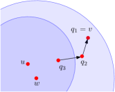
Figure 9: The partial path constructed backwards from $v$. Setting $q_{4}=u$ will complete it.

Let $c$ be the constant from the spanner construction of Section 3.2, and recall that we scale $P$ such that the smallest radius is $c$. Suppose that we have $q_{1},\dots,q_{k}$ and that $wq_{k}$ is not an edge of $H$ (otherwise we could finish by setting $u=w$). Let $\sigma,\tau\in\operatorname{\mathcal{Q}}_{0}$ be the cells such that $w\in\tau$ and $q_{k}\in\sigma$. We distinguish two cases, depending on $d(\sigma,\tau)$, and we either show how to find $u$ to complete the path from $u$ to $v$ or how to choose $q_{k+1}$.

Case 1: $d(\sigma,\tau)<c-2$. Let $Q=(P\cap\sigma)\cup(P\cap\tau)$. We have that $w,q_{k}\in Q$. The algorithm of Section 3.2 constructs a Euclidean spanner for $Q$ and adds its edges to $H$. In particular, there is a directed path $\pi$ from $w$ to $q_{k}$ that uses only sites of $Q$. By construction, the pairwise distances between the sites of $Q$ are all at most $c$. Thus, for each $p\in Q$ we have $p\in D(w)$ and $q_{k}\in D(p)$, and therefore $i\leq d_{h}(s,p)\leq i+1$. We set $u$ be the last site of $\pi$ with $d_{h}(s,u)=i$. To obtain the desired path from $u$ to $v$ we take the subpath of $\pi$ starting at $u$ and concatenate it to the the partial path $q_{k},\dots,q_{1}=v$.

Case 2: $d(\sigma,\tau)\geq c-2$. Since $wq_{k}$ is not an edge of $H$, by Lemma 3.7 there exists an edge $rq_{k}$ in $H$ with $|wr|<|wq_{k}|$. We set $q_{k+1}=r$. Since $q_{k}\in D(w)$, we have $q_{k+1}\in D(w)$ and $i\leq d_{h}(s,q_{k+1})\leq i+1$. If $d_{h}(s,q_{k})=i$, we set $u=q_{k+1}$ and are done. Otherwise, $q_{k+1}$ satisfies properties (i)–(iii) and we continue to extend the path.

Since the distance to $w$ decreases in each step and since $P$ is finite, this process eventually stops and the lemma follows. ∎

1 $W_{0}\leftarrow\{s\}$; $\operatorname{d}[s]=0$; $\pi[s]=s$; $i=0$; and, for $p\in P\setminus\{s\}$, $\operatorname{d}[p]=\infty$ and $\pi[p]=\operatorname{NIL}$

2 while $W_{i}\neq\emptyset$ do

3       compute power diagram with point location structure $\operatorname{PD}_{i}$ of $W_{i}$

4       queue $Q\leftarrow W_{i}$ ; $W_{i+1}\leftarrow\emptyset$

5       while $Q\neq\emptyset$ do

6             $p\leftarrow\text{dequeue}(Q)$

7             foreach edge $pq$ of $H$ do

                   $u\leftarrow\operatorname{PD}_{i}(q)$ // query $\operatorname{PD}_{i}$ with $q$, $D(u)$ minimizes the power distance from $q$

8                   if $q\in D(u)$ and $\operatorname{d}[q]=\infty$ then

9                         $\text{enqueue}(Q,q)$; $\operatorname{d}[q]=i+1$; $\pi[q]=u$; add $q$ to $W_{i+1}$

10      $i\leftarrow i+1$

Algorithm 5 Computing the BFS tree for $G$ with root $s$ using the spanner $H$.

The BFS tree for $s$ is computed iteratively; see Algorithm 5 for pseudocode. Initially, we set $W_{0}=\{s\}$. Now assume we have computed $W_{0},\ldots,W_{i}$. By Lemma 4.1, all sites in $W_{i+1}$ can be reached from $W_{i}$ in the subgraph of $H$ induced by $W_{i}\cup W_{i+1}$. Thus, we can compute $W_{i+1}$ by running a BFS search in $H$ from the points of $W_{i}$ using a queue $Q$. Every time we encounter a new vertex $q$, we check if it lies in a disk around a site of $W_{i}$, and is not yet in the BFS tree for $s$. If so, we add $q$ to $W_{i+1}$ and to $Q$. Otherwise, we discard $q$. To test whether $q$ lies in a disk of $W_{i}$, we compute a power diagram for $W_{i}$ in time $O(|W_{i}|\log|W_{i}|)$ and query it with $q$.

A site $p$ at level $i$ is traversed by at most two BFS searches in $H$. In the first search we discover that $p$ is in $W_{i}$, and in the second search $p$ is a starting point — this is the search to discover $W_{i+1}$. It follows that an edge $pq$ of $H$ is considered twice by Algorithm 5. Each time we consider the edge $pq$ we spend $O(\log n)$ time for querying a power diagram with $q$. Since $H$ is sparse, the total time required is $O(n\log n)$. This establishes the following theorem.

Theorem 4.2.

Let $P\subset\mathbb{R}^{2}$ be a set of $n$ points. Given a spanner $H$ for the transmission graph $G$ of $P$ as in Theorem 3.1, Theorem 3.12, or Theorem 3.18, we can compute in $O(n\log n)$ additional time a BFS tree in $G$ rooted at any given site $s\in P$.

4.2 Geometric Reachability Oracles

Let $G$ be a directed graph. If there is a directed path from a vertex $s$ to a vertex $t$ in $G$, we say $s$ can reach $t$ (in $G$). A reachability oracle for a graph $G$ is a data structure that can answer efficiently for any given pair $s$, $t$ of vertices of $G$ whether $s$ can reach $t$. Reachability oracles have been studied extensively over the last decades (see, e.g., [14, 26] and the references therein).

When $G$ is a transmission graph we are interested in a more general type of reachability query where the target $t$ is not necessarily a vertex of $G$, but an arbitrary point in the plane. We say that a site $s$ can reach a point $t\in\mathbb{R}^{2}$ if there is a site $q$ in $G$ such that $t\in D(q)$ and such that $s$ can reach $q$ in $G$. We call a data structure that supports this type of queries a geometric reachability oracle. We can use our spanner construction from Theorem 3.12 to extend any reachability oracle for a transmission graph to a geometric reachability oracle with a small overhead in space and query time. More precisely, we prove the following theorem.

Theorem 4.3.

Let $P$ be a set of $n$ points in the plane with radius ratio $\Psi$. Given a reachability oracle for the transmission graph $G$ of $P$ that requires $S(n)$ space and has query time $Q(n)$, we can obtain in $O(n\log n\log\Psi)$ time a geometric reachability oracle for $G$ that requires $S(n)+O(n\log\Psi)$ space and can answer a query in $O(Q(n)+\log n\log\Psi)$ time.

Given a query $s,t$ with a target $t\in\mathbb{R}^{2}$, our strategy is to find a small subset $Q\subseteq P$ such that for each $q\in Q$, $t\in D(q)$, and $Q$ “covers the space around $t$” in the following sense. For any disk $D(p)$ such that $t\in D(p)$ there is a site $q\in Q$ with $q\in D(p)$. In particular the edge $pq$ is in $G$.

Such a set $Q$ satisfies that $s$ can reach $t$ if and only if $s$ can reach some site $q\in Q$. Once we have computed $Q$ we decide whether $s$ can reach $t$ by querying the given reachability oracle with $s,q$ for all $q\in Q$. The answer is positive if and only if it is positive for at least one site $q\in Q$.

In what follows, we construct a data structure of size $O(n\log\Psi)$ that allows to find such a set $Q$ of size $O(1)$ in $O(\log n\log\Psi)$ time. Theorem 4.3 is then immediate.

The Data Structure.

We compute a $2$-spanner $H$ for $G$ as in Theorem 3.12. Let $k$ (the number of cones) and $c$ (the separation parameter) be the two constants used by the construction of $H$, and recall that we scaled $P$ such that the smallest radius of a site in $P$ is $c$. Let $T$ be the quadforest used by the construction of $H$. The trees in $T$ have depth $O(\log\Psi)$ and each node $v\in T$ corresponds to a grid cell $\sigma_{v}$ from some grid $\operatorname{\mathcal{Q}}_{i}$, $i\geq 0$. Our data structure is obtained by augmenting each node $v\in T$ by a power diagram $\operatorname{PD}_{\sigma_{v}}$ for the sites in $\sigma_{v}\cap P$, together with a point location data structure. This requires $O(|\sigma_{v}\cap P|)$ space and $O(|\sigma_{v}\cap P|\log|\sigma_{v}\cap P|)$ time [15, 20] for each $v$. Since any site of $P$ is in $O(\log\Psi)$ cells of $T$, we need $O(n\log\Psi)$ space and $O(n\log n\log\Psi)$ time in total.

1 $L\leftarrow$ depth of $T$

2 for $i=0,\dots,L$ do

3       $\sigma\leftarrow$ cell of $\operatorname{\mathcal{Q}}_{i}$ with $t\in\sigma$

4       foreach $\tau\in N(\sigma)$ contained in $C_{\sigma}^{2}$ do

             $q\leftarrow\operatorname{PD}_{\tau}(t)$ // query $\operatorname{PD}_{\tau}$ with $t$

5             if $t\in D(q)$, add $q$ to $Q$

6      Stop if at least one $q$ was added to $Q$

Algorithm 6 Query Algorithm for a cone $C$ and a point $t$.

Performing a Query.

Let a query point $t\in\mathbb{R}^{2}$ be given. Let $\sigma$ be the cell in $\operatorname{\mathcal{Q}}_{0}$ that contains $t$. To find $Q$, we first traverse all non-empty cells $\tau\in\operatorname{\mathcal{Q}}_{0}$ with $d(\sigma,\tau)\leq c-2$. From each such cell $\tau$, if there exists a site $q\in\tau\cap P$ such that $t\in D(q)$ then we add one, arbitrary, such site to $Q$. To determine if such a site exists, and to find one if it exists, we query $\operatorname{PD}_{\tau}$ with $t$. Second, we go through all cones $C\in{\mathcal{C}}$, and we run Algorithm 6 with $C$ and $t$ to find the remaining sites for $Q$. Algorithm 6 is similar to Algorithms 1 and 2, and computes the incoming edge of $t$ if it would have been inserted into the spanner. We go through the grids at all levels of $T$. For each level we consider the cell $\sigma$ that contains $t$ and for each cell $\tau\in N(\sigma)$ that is contained in $C_{\sigma}^{2}$ we select a site with an edge to $t$ if there is one. Lemma 3.7 holds for the incoming edges of $t$ and using this fact, we can prove that our data structure has the desired properties.

Lemma 4.4.

Let $P$ be a set of $n$ points in the plane with radius ratio $\Psi$. We can construct in $O(n\log n\log\Psi)$ time a data structure that finds for any given query point $t\in\mathbb{R}^{2}$ a set $Q\subseteq P$ such that $|Q|=O(1)$ and for any site $p\in P$, if $t\in D(p)$ we have that $D(p)\cap Q\neq\emptyset$. The query time is $O(\log n\log\Psi)$ and the space requirement is $O(n\log\Psi)$.

Proof.

The construction time and the space requirement are immediate. For the query time recall that $T$ has depth $O(\log\Psi)$ and by Lemma 3.3, at each level we make $O(c^{2})$ queries to the power diagrams. It follows that it takes $O(\log n\log\Psi)$ time to compute $Q$.

By construction, $Q$ has size $O(1)$. Indeed, at the first step, we add at most one site for every cell of distance at most $c-2$ from $\sigma$, and there are $O(c^{2})$ such cells. In the second step, for each cone, we only add sites from $O(c^{2})$ cells at one level of $T$.

Now let $p\in P$ be a site with $t\in D(p)$. It remains to show that $D(p)\cap Q\neq\emptyset$. If $p\in Q$, we are done. If not, we let $\sigma$ and $\tau$ be the cells in $\operatorname{\mathcal{Q}}_{0}$ with $t\in\sigma$ and $p\in\tau$. If $d(\sigma,\tau)\leq c-2$ then there must be a site $q\in\tau\cap Q$. Since $\operatorname{diam}(\tau)=1$ and $r_{p}\geq c$, we have $q\in D(p)$. If $d(\sigma,\tau)>c-2$ then since $pt$ is an edge in $G$ that is not selected by Algorithm 6, Lemma 3.7 guarantees that there is an edge $qt$ with $q\in Q$ and $|pq|<|pt|$. Since $t\in D(p)$ we also have $q\in D(p)$. This finishes the proof. ∎

5 Conclusion

We have described the first construction of spanners for transmissions graphs that runs in near-linear time, and we demonstrated its usefulness by describing two applications. Our techniques are quite general, and we expect that they will be applicable in similar settings. For example, in an ongoing work we consider how to extend our results to (undirected) disk intersection graphs. This would significantly improve the bounds of Fürer and Kasiviswanathan [12].

Our most general spanner construction requires a dynamic data structure for planar Euclidean nearest neighbors. It is an interesting challenge to find a simpler solution that possibly avoids the need for such a structure.

Finally, we believe that our work indicates that transmission graphs constitute an interesting and fruitful model of geometric graphs worthy of further investigation. In a companion paper [17], we consider several questions concerning reachability in transmission graphs. In particular, we describe several constructions of reachability oracles for transmission graphs (see Section 4.2), providing many opportunities to apply Theorem 4.3. Also, in this context our spanner construction plays a crucial role in obtaining fast preprocessing algorithms.

Acknowledgments.

We like to thank Paz Carmi and Günter Rote for valuable comments. We also thank the anonymous referees for their careful reading of the paper and for their insightful suggestions, and in particular for pointing out the problem of geometric reachability queries as described in Section 4.2.

References

- [1] P. Afshani and T. M. Chan. Optimal halfspace range reporting in three dimensions. In Proc. 20th Annu. ACM-SIAM Sympos. Discrete Algorithms (SODA), pages 180–186, 2009.
- [2] M. de Berg, O. Cheong, M. van Kreveld, and M. H. Overmars. Computational Geometry: Algorithms and Applications. Springer-Verlag, 3rd edition, 2008.
- [3] P. Bose, M. Damian, K. Douïeb, J. O’Rourke, B. Seamone, M. H. M. Smid, and S. Wuhrer. -angle Yao graphs are spanners. Internat. J. Comput. Geom. Appl., 22(1):61–82, 2012.
- [4] A. Boukerche. Algorithms and Protocols for Wireless Sensor Networks. Wiley Series on Parallel and Distributed Computing. Wiley-IEEE Press, 1st edition, 2008.
- [5] S. Cabello and M. Jejĉiĉ. Shortest paths in intersection graphs of unit disks. Comput. Geom., 48(4):360–367, 2015.
- [6] P. B. Callahan and S. R. Kosaraju. A decomposition of multidimensional point sets with applications to -nearest-neighbors and -body potential fields. J. ACM, 42(1):67–90, 1995.
- [7] P. Carmi, 2014. personal communication.
- [8] T. M. Chan. A dynamic data structure for 3-D convex hulls and 2-D nearest neighbor queries. J. ACM, 57(3):Art. 16, 15, 2010.
- [9] T. M. Chan and K. A. Tsakalidis. Optimal deterministic algorithms for 2-d and 3-d shallow cuttings. In Proc. 31st Int. Sympos. Comput. Geom. (SoCG), pages 719–732, 2015.
- [10] M. S. Chang, N. F. Huang, and C. Y. Tang. An optimal algorithm for constructing oriented Voronoi diagrams and geographic neighborhood graphs. Inform. Process. Lett., 35(5):255–260, 1990.
- [11] B. N. Clark, C. J. Colbourn, and D. S. Johnson. Unit disk graphs. Discrete Math., 86(1-3):165–177, 1990.
- [12] M. Fürer and S. P. Kasiviswanathan. Spanners for geometric intersection graphs with applications. J. Comput. Geom., 3(1):31–64, 2012.
- [13] S. Har-Peled. Geometric Approximation Algorithms. American Mathematical Society, 2011.
- [14] J. Holm, E. Rotenberg, and M. Thorup. Planar reachability in linear space and constant time. In Proc. 56th Annu. IEEE Sympos. Found. Comput. Sci. (FOCS), pages 370–389, 2015.
- [15] H. Imai, M. Iri, and K. Murota. Voronoi diagram in the Laguerre geometry and its applications. SIAM J. Comput., 14(1):93–105, 1985.
- [16] H. Kaplan, W. Mulzer, L. Roditty, and P. Seiferth. Spanners and reachability oracles for directed transmission graphs. In Proc. 31st Int. Sympos. Comput. Geom. (SoCG), pages 156–170, 2015.
- [17] H. Kaplan, W. Mulzer, L. Roditty, and P. Seiferth. Reachability oracles for directed transmission graphs. arXiv:1601.07797, 2016.
- [18] H. Kaplan, W. Mulzer, L. Roditty, P. Seiferth, and M. Sharir. Dynamic planar Voronoi diagrams for general distance functions and their algorithmic applications. In Proc. 28th Annu. ACM-SIAM Sympos. Discrete Algorithms (SODA), pages 2495–2504, 2017.
- [19] K. Kedem, R. Livne, J. Pach, and M. Sharir. On the union of Jordan regions and collision-free translational motion amidst polygonal obstacles. Discrete Comput. Geom., 1:59–70, 1986.
- [20] D. Kirkpatrick. Optimal search in planar subdivisions. SIAM J. Comput., 12(1):28–35, 1983.
- [21] M. Löffler and W. Mulzer. Triangulating the square and squaring the triangle: quadtrees and Delaunay triangulations are equivalent. SIAM J. Comput., 41(4):941–974, 2012.
- [22] G. Narasimhan and M. H. M. Smid. Geometric spanner networks. Cambridge University Press, 2007.
- [23] D. Peleg and L. Roditty. Localized spanner construction for ad hoc networks with variable transmission range. ACM Transactions on Sensor Networks (TOSN), 7(3):25:1–25:14, 2010.
- [24] F. P. Preparata and M. I. Shamos. Computational geometry. An introduction. Springer-Verlag, 1985.
- [25] M. Sharir and P. K. Agarwal. Davenport-Schinzel sequences and their geometric applications. Cambridge University Press, 1996.
- [26] M. Thorup. Compact oracles for reachability and approximate distances in planar digraphs. J. ACM, 51(6):993–1024, 2004.
- [27] P. von Rickenbach, R. Wattenhofer, and A. Zollinger. Algorithmic models of interference in wireless ad hoc and sensor networks. IEEE/ACM Transactions on Networking, 17(1):172–185, 2009.
- [28] A. C.-C. Yao. On constructing minimum spanning trees in -dimensional spaces and related problems. SIAM J. Comput., 11(4):721–736, 1982.