Dynamical friction for supersonic motion
in a homogeneous gaseous medium

Abstract

Context. The supersonic motion of gravitating objects through a gaseous ambient medium constitutes a classical problem in theoretical astrophysics. Its application covers a broad range of objects and scales from planetesimals, planets, all kind of stars, up to galaxies and black holes. Especially the dynamical friction, caused by the forming wake behind the object, plays an important role for the dynamics of the system. To calculate the dynamical friction for a particular system, standard formulae, based on linear theory are often used.

Aims. It is our goal to check the general validity of these formulae and provide suitable expressions for the dynamical friction acting on the moving object, based on the basic physical parameters of the problem, namely the mass, radius, and velocity of the perturber, the gas mass density, soundspeed, and adiabatic index of the gaseous medium, and the size of the forming wake or interaction time, respectively.

Methods. We perform dedicated sequences of high resolution numerical studies of rigid bodies moving supersonically through a homogeneous ambient medium, and calculate the total drag acting on the object, which is the sum of gravitational and hydrodynamical drag. We study cases without gravity with purely hydrodynamical drag, as well as gravitating objects. In various numerical experiments, we determine the drag force acting on the moving body and its dependence on the basic physical parameters of the problem, as given above. From the final equilibrium state of the simulations, we compute for gravitating objects the dynamical friction by direct numerical integration of the gravitational pull acting on the embedded object.

Results. The numerical experiments confirm the known scaling laws for the dependence of the dynamical friction on the basic physical parameters as derived in earlier semi-analytical studies. As a new important result we find that the shock’s stand-off distance is revealed as the minimum spatial interaction scale of dynamical friction. Below this radius, the gas settles into a hydrostatic state, which – due to its spherical symmetry – causes no net gravitational pull onto the moving body. Finally, we derive an analytic estimate for the stand-off distance that can used conveniently in calculating the dynamical friction force.

1 Introduction

The motion of gravitating objects through a gaseous ambient medium is a classical problem in theoretical astrophysics. Of special interest is the force acting on the object as it determines typical evolution or equilibration time scales. This force is caused by two main mechanisms, the purely hydrodynamic drag, and by dynamical friction. Even without gravity, the flow of the gas will be perturbed by the body because it acts as an obstacle and blocks the gas in front of it. This causes an exchange of momentum between the embedded body and the surroundings, leading to a hydrodynamic drag force on the object. On earth this gives for example rise to the air resistance of all flying objects, a drag force that tends to oppose the motion of the body. In an astrophysical setting, for a moving massive body its gravitational attraction onto the surrounding leads to the formation of a wake of higher-than-average density behind the moving object, and, as a result, to a gravitational pull of the dense region onto the body. This additional force is again directed opposite to the motion of the body and leads to a slow down. This force is usually called gravitational drag force or dynamical friction (Chandrasekhar, 1943; Ostriker, 1999). Hence, the total drag force acting on a gravitating body is the sum of the hydrodynamic drag and dynamical friction.

Its astrophysical application covers a wide range of fields, as pointed out recently by Lee & Stahler (2014). In the common envelope phase, the decay time of the secondary companion is driven by dynamical friction (Ricker & Taam, 2008, 2012), as well as the important survival rate of planets around evolved stars (Villaver & Livio, 2009). Further applications include the settling of massive stars in molecular clouds (Chavarría et al., 2010), the drag on a star in the accretion flow around black holes (Narayan, 2000), the coalescence of black holes (Armitage & Natarajan, 2005), and the migration of planetesimals (Grishin & Perets, 2015). In the framework of planet evolution, dynamical friction plays a role in the change of planetary inclination due to the interaction with the disk (Rein, 2012; Teyssandier et al., 2013). The dynamical interactions of evolved stars that move through the interstellar medium (ISM) determine the observational properties of the dust in the envelope (Slavin et al., 2004; van Marle et al., 2011; Meyer et al., 2014a, b, 2015).

This incomplete list of applications shows that the phenomenon of dynamical friction is widespread and of general importance. But still, there is no satisfying derivation of the force on the object, despite many years of research (see e.g. Lee & Stahler, 2014). In this study, we tackle this important problem of dynamical friction via direct numerical modeling. We perform hydrodynamical simulations of a gravitating body moving supersonically through a homogeneous medium and extract the dynamical friction on the object. We analyze in detail the scaling of the drag with important physical parameter of the problem such as Mach number and mass of the object and others, and compare this to existing formulae for dynamical friction.

The paper is organized as follows: In Sect. 2, we summarize the status on formulae for dynamical friction. In Sect. 3, we describe the hydrodynamics equations and the physical and numerical setup of the simulations. In Sect. 4, we present comparison simulations to laboratory experiments for non-gravitating objects, moving at supersonic speed through air. In Sect. 5, we present the simulations of gravitating objects for various different physical parameter and discuss their implication on the dynamical friction. In Sect. 6, we present a new formula for the drag force. In Sect. 7, we give a brief summary of the study.

2 Analytical estimates of dynamical friction

A first account of dynamical friction has been given by Chandrasekhar (1943) who calculated the dynamical friction of a star embedded in a stellar cluster. His results were later adapted to the motion of stars through the ISM or galaxies through the intergalactic medium. Here, the ambient gas is typically treated as a static hydrodynamic continuum which is transversed by a moving body of mass $M$ and the velocity $V_{\infty}$. Using the impulse approximation, where the moving mass perturbs the surroundings only for a finite time, Ruderman & Spiegel (1971) derived a general formula for the dynamical friction force $F_{\mathrm{DF}}$ acting on the mass $M$:

$$F_{\mathrm{DF}}=4\pi\rho_{\infty}\left(\frac{GM}{V_{\infty}}\right)^{2}\,C_{A}\,.$$ (1)

In Eq. (1), $\rho_{\infty}$ denotes the ambient constant density, $G$ is the gravitational constant, and $C_{A}$ stands for the “Coulomb logarithm”

$$C_{A}=\ln\left(s_{\mathrm{max}}/s_{\mathrm{min}}\right)\,,$$ (2)

where $s_{\mathrm{min}}$ and $s_{\mathrm{max}}$ correspond to the minimum and maximum impact parameter of the interaction. A very similar expression for the drag on a star moving in a zero temperature medium has been derived by Bondi & Hoyle (1944) who analyzed the change in momentum by the gas that is collected in a very thin line behind the object. Additionally, they derived relations for the gas accretion rate onto the body.

To apply Eq. (1) to various physical problems, the relevant length scales $s_{\mathrm{min}}$ and $s_{\mathrm{max}}$ need to be known. Typically, for $s_{\mathrm{max}}$ the maximum extension of the medium, or a characteristic (global) length scale is assumed. For the minimum length, $s_{\mathrm{min}}$, the situation is not so clear and no general accepted recipe exists. Often, either the physical radius $R$ of the object is chosen or, in case the body becomes very small, $s_{\mathrm{min}}\approx\max{(R,R_{\mathrm{A}})}$. Here $R_{\mathrm{A}}$ stands for the accretion radius

$$R_{\mathrm{A}}=\frac{2GM}{V_{\infty}^{2}}\,.$$ (3)

Recently, Cantó et al. (2011) derived an approximation for $s_{\mathrm{min}}$ using ballistic orbit theory, which does not account for the pressure, however. Obviously, the question of the correct minimum radius of the object is still not clarified and remains ambiguous.

While Eq. (1) was derived for a pressureless medium (dust), some corrections have to be applied in case pressure effects play a role. In the supersonic case, with $V_{\infty}>c_{\infty}$, where $c_{\infty}$ denotes the soundspeed of the unperturbed medium, a bow shock forms in front of the object where (additional) energy can be dissipated. Using the linearized fluid equations Ruderman & Spiegel (1971) and Rephaeli & Salpeter (1980) derive a correction to the above equation that depends on the Mach number of the object.

In an important work, Ostriker (1999) extended the above analysis and studied the time-dependent dynamical friction force acting on a massive object embedded into a gaseous medium in the sub- and supersonic regime. Her analysis resulted in an expression for the coefficient $C_{A}$, very similar to that of Rephaeli & Salpeter (1980), which includes a time-dependent maximum radius, $s_{\mathrm{max}}\sim V_{\infty}t$, where $t$ is the time the object has interacted with the gas. Her analysis is based on linear perturbation theory and useful to study time-dependent phenomena. The expression for the supersonic case reads

$$C_{A}=\ln\left[\frac{V_{\infty}t}{s_{\mathrm{min}}}\,\left(\frac{\mathcal{M}^{2}-1}{\mathcal{M}^{2}}\right)^{1/2}\right]\leavevmode\nobreak\ ,$$ (4)

where $\mathcal{M}=V_{\infty}/c_{\infty}$ denotes the Mach number of the problem. Obviously, if we set $s_{max}=V_{\infty}t$, then Eqs. (2) and (4) agree with each other in the limit of large $\mathcal{M}$, because for highly supersonic flows pressure effects become less important. Here, we are not interested in the time-dependent process but will focus on the final stationary state.

In addition to these analytic estimates there have been many numerical studies of moving gravitating objects embedded in a gas. The first to address this issue numerically was Hunt (1971) who used a special shock fitting method to calculate the flow around the body and the accretion rate onto it. Later, Shima et al. (1985) were the first to use modern type fluid dynamical methods on this problem and performed axisymmetric simulations in spherical polar coordinates. In their now classic paper they studied the drag force and the accretion rate onto the object as a function of the velocity and found very rough qualitative agreement with Eqs. (1) and (2), when using for $s_{\mathrm{min}}$ the inner radius of the computational domain. Most of the subsequent simulations dealt with open inner boundary conditions and focused on the mass accretion rate onto the object. An introductory summary to this so called Bondi-Hoyle-Littleton accretion process is given in the review article by Edgar (2004). In this paper we will not study accretion onto the object and study rigid bodies only. The main focus will lie on the accurate computation of the dynamical friction and – as a pre-requisite – on the determination of the minimum integration radius $s_{\mathrm{min}}$.

The validity of the formula by Ostriker has been demonstrated by Sánchez-Salcedo & Brandenburg (2001) who showed agreement for moderate Mach numbers in non-linear, isothermal simulations. However, they used a Plummer-type potential with a smoothing length much larger than $R_{\mathrm{A}}$. Later, Kim & Kim (2009) reanalyzed dynamical friction for extended bodies through numerical simulations. However, they did not consider objects with a more or less rigid surface (like stars) but used again a Plummer-type potential with a smoothing length, and hence their results may be applicable more to galaxies moving in the intergalactic medium. They compare their results to the formula by Ostriker (1999) and provide a new fitting formula involving $R_{\mathrm{A}}$. They used an axisymmetric cylindrical coordinate system, which suffers in terms of limited resolution close to the center.

Starting with Ruffert (1994) and Ruffert & Arnett (1994) there have been many simulations considering the three-dimensional flow around an accreting object. An interesting feature discovered already in these first studies is the onset of unstable flow when breaking the axial symmetry, an effect that is most pronounced in planar two-dimensional flows, that are nonphysical however. A comprehensive summary of two-dimensional (2D) and three-dimensional (3D) simulations carried out has been given by Foglizzo et al. (2005). They point out that the origin of the instability, i.e. under what conditions it is expected and its effect on the drag force, are still not understood. In this paper we will avoid the question of instability and focus on purely axisymmetric flows.

It will be useful to compare the drag formula Eq. (1) to standard hydrodynamic drag formula. From dimensional analyses (Landau & Lifshitz, 1966) one finds for the hydrodynamical drag force acting on an object with cross section $A$

$$F_{\mathrm{hydro}}=\frac{1}{2}\,C_{D}\,\rho_{\infty}\,V_{\infty}^{2}\,A.$$ (5)

The dimensionless drag coefficient $C_{\mathrm{D}}$ contains the details of how the body and the medium physically interact with each other, e.g. through surface effects and the dependence on laminar vs. turbulent flows. If we use the accretion radius to set the interaction cross section $A=\pi R_{A}^{2}$, the ratio of the hydrodynamical drag and the dynamical friction is given by:

$$\frac{F_{\mathrm{hydro}}}{F_{\mathrm{DF}}}=\frac{C_{D}}{2C_{A}}$$ (6)

In this study, we determine the dependence of dynamical friction acting on a rigid, gravitating body moving supersonically through a homogeneous medium on the basic physical parameters of the system. First, we demonstrate that the dynamical friction scales like Eq. (1) and we derive an analytic relation for the up-to-now undetermined minimum length scale $s_{\mathrm{min}}$ of the problem, and finally give a convenient expression for the dynamical friction in general.

3 Physics and numerics

3.1 Problem setup

We model gravitating, spherical objects with a given mass $M$ and radius $R$ moving with supersonic speed $V_{\infty}$ through a homogeneous medium, that is characterized by its mass density $\rho_{\infty}$, pressure $p_{\infty}$, and temperature $T_{\infty}$ or soundspeed $c_{\infty}$, respectively. As initial condition, the object is placed instantaneously into the ambient medium and the evolution of the gaseous system is followed using time-dependent hydrodynamical simulations. After the system reaches a steady state we determine the gravitational pull of the gas onto the object (the dynamical friction) as well as the hydrodynamic drag.

3.2 Equations

We study the motion of the ideal gas by solving the Euler equations

$$\frac{\partial\rho}{\partial t}+\nabla\cdot(\rho\@vec{u}) =0$$ (7)

$$\frac{\partial}{\partial t}\rho\@vec{u}+\nabla\cdot(\rho\@vec{u}\otimes\@vec{u})+\nabla p =\rho\,\@vec{a}_{\mathrm{ext}}$$ (8)

$$\frac{\partial e}{\partial t}+\nabla\cdot[(e+p)\@vec{u}] =\rho\,\@vec{u}\cdot\@vec{a}_{\mathrm{ext}}.$$ (9)

Here, $\rho$ denotes the gas mass density, $\@vec{u}$ the velocity, $p$ the gas pressure, and $e=e_{\mathrm{kin}}+e_{\mathrm{th}}$ the total (kinetic and thermal) energy density of the gas. The acceleration due to external forces $\@vec{a}_{\mathrm{ext}}$ is given here by the gravitational attraction of the moving object

$$\@vec{a}_{\mathrm{ext}}=-\frac{GM}{r^{2}}\@vec{e}_{r}$$ (10)

where $r$ is the distance from the center of the object to the position under consideration. We close the equations of hydrodynamics with the ideal gas equation of state

$$p=(\gamma-1)e_{\mathrm{th}}\,.$$ (11)

Gas pressure, density, and temperature are related via

$$p=\frac{k_{\mathrm{B}}}{\mu\leavevmode\nobreak\ m_{\mathrm{H}}}\rho T\,,$$ (12)

where $\mu$ is the mean molecular weight, $k_{\mathrm{B}}$ the Boltzmann constant and $m_{\mathrm{H}}$ the mass of the hydrogen atom. The soundspeed of the gas is given by

$$c_{\infty}=\sqrt{\gamma\frac{p}{\rho}}.$$ (13)

In our simulations we use a constant value of the adiabatic exponent $\gamma$. We study the influence of different $\gamma$-values on the dynamical friction in dedicated parameter series, see Sect. 5.7.

From the given values of the density $\rho_{\infty}$ and pressure $p_{\infty}$ of the initially homogeneous medium, its adiabatic index $\gamma$, and the speed $V_{\infty}$ of the moving object, the associated Mach number of the system is given as

$${\cal M}=V_{\infty}/c_{\infty}.$$ (14)

3.3 Numerics

Simulations are carried out using the open-source code PLUTO (Mignone et al., 2007), version 4. Part of the simulations were carried out with a new in-house developed CUDA version for usage on GPUs. We use a Runge-Kutta time stepping scheme of second order with a second order reconstruction of states in space, a van-Leer limiter in the reconstruction step, and a Harten-Lax-van Leer solver for the Riemann-Problem.

Equations (7) to (9) are solved in the co-moving frame of the object, i.e. the object is at rest in the modeling frame and the initial velocity of the surrounding homogeneous gas corresponds to the physical speed of the solid body. We use a 2D spherical grid $(r,\theta)$ assuming axial symmetry. The object is fixed at the origin of the coordinate system and the gas flows into the negative $z$-direction. The solid surface of the moving spherical object is represented as boundary conditions at the radial inner boundary of the computational domain. Here, we use reflecting boundary conditions, corresponding to a non-accreting object. The computational domain extends in the radial direction from the radius $R$ of the object up to $R_{\mathrm{domain}}=100\mbox{ or }1000\leavevmode\nobreak\ R$. The symmetry axis of the domain is aligned with the trajectory of the object. In the polar direction, the computational domain extends from $0$ to $\pi$ using a grid spacing uniform in angle. To obtain high resolution at the interesting area around the object, and to ensure an approximately quadratic grid spacing in the radial and the polar direction of each grid cell, we use a logarithmic grid spacing in the radial direction.

At the outer radial boundary $R_{\mathrm{domain}}$, we set the boundary conditions according to the gas flow of the surrounding: In the upper hemisphere (for $\theta\in[0,\pi/2]$), we implemented an inflow boundary condition, i.e. all ghost cells are set to the unperturbed values of the surrounding medium. In the lower hemisphere (for $\theta\in[\pi/2,\pi]$), we implemented a zero-gradient boundary condition so that the out-flowing material can leave the computational domain without reflections. As already mentioned, we perform simulations in axial symmetry and therefore at $\theta=0$ (positive $z$-axis) and at $\theta=\pi$ (negative $z$-axis) we make use of axisymmetric boundary conditions.

Simulations with a size of the body of $R=0.1\mbox{ R}_{\odot}$ are performed on a grid consisting of $700\times 480$ grid cells, simulations with a smaller size of the body of $R=0.01\mbox{ R}_{\odot}$ are performed on a grid consisting of $860\times 400$ grid cells. We present a corresponding convergence study in detail in appendix C.

3.4 Assumptions and simplifications

The numerical experiments are performed to determine the dynamical friction in a general astrophysical context. Hence, we do not take into account effects, which depend on a specific system under investigation, such as radiative heating and cooling. The flow is assumed to be inviscid. Self-gravity of the gas is not taken into account. Effects of magnetic fields are not investigated. The long-evolution problem of a time-dependent slow-down of the moving body by the acting dynamical friction is not included in this study, see Sánchez-Salcedo & Brandenburg (2001) for a discussion on this issue. The formula for dynamical friction is derived within the co-moving frame of the moving body. The object is treated as a rigid body where no accretion through its surface is allowed. The medium is considered to behave as an ideal gas.

3.5 Calculation of the drag force

The total drag force acting on an object moving through an ambient medium can be calculated from the momentum balance in the final equilibrium state (Landau & Lifshitz, 1966). In our case, the object is moving along the $z$-direction and we have to consider the $z$-component of Eq. (8) which reads in equilibrium

$$\nabla\cdot(\rho u_{z}\@vec{u})+\frac{\partial p}{\partial z}-\rho a_{z}=0\,,$$ (15)

where $a_{z}$ denotes the $z$-component of the gravitational acceleration due to the moving object. Integrating over the whole volume of the computational domain we can convert the first two parts into surface integrals and obtain

$$\int_{\mathrm{in}}\left[(\rho u_{z}\@vec{u})+p\@vec{n}\right]\cdot\@vec{df}+\int_{\mathrm{Vol}}\rho a_{z}dV+\int_{\mathrm{out}}\left[(\rho u_{z}\@vec{u})+p\@vec{n}\right]\cdot\@vec{df}=0\,,$$ (16)

where $\@vec{df}$ is the surface element and $dV$ the volume element, and the subscript $in$ and $out$ refer to the inner and outer boundary of the computational domain. The first term of Eq. (16) represents the total hydrodynamical force acting on the surface of the body which is the sum of a momentum transport, $F^{\mathrm{tra}}_{in}$, through the body’s surface (e.g. for porous objects or open, accreting bodies) and a pressure force, $F^{\mathrm{prs}}_{in}$, acting directly on the body. The second term is the dynamical friction force on the body, $F_{\mathrm{DF}}$, which is obtained by integrating over the whole volume of the domain. The sum of these two contributions must be balanced by the corresponding momentum transport and pressure terms at the outer boundary, $F^{\mathrm{tra}}_{\mathrm{out}}$ and $F^{\mathrm{prs}}_{\mathrm{out}}$, respectively. In our case, the first surface integral in Eq. (16) is taken at the surface of the moving object, here the radius, $R$, of the spherical body, and the last surface integral at the outer boundary of the domain, $R_{\mathrm{domain}}$. In the case of an impermeable rigid body, $F^{\mathrm{tra}}_{in}=0$, and we obtain the final force balance as

$$F^{\mathrm{prs}}_{\mathrm{in}}+F_{\mathrm{DF}}+F^{\mathrm{tra}}_{\mathrm{out}}+F^{\mathrm{prs}}_{\mathrm{out}}=0\,.$$ (17)

We calculate all these forces for our simulations and evaluate the importance of the different contributions. Eq. (17) shows that the drag acting on an object can be either evaluated at the inner boundary (plus gravity) or solely at the outer boundary.

4 Comparison to laboratory experiments

In computational astrophysics, it is only rarely possible to test the numerical algorithms against laboratory experiments. However, in the case of the problem on hand – a sphere moving supersonically through a gaseous medium – experimental data is available for non-gravitating moving bodies. To check the validity of our numerical ansatz and prove the accuracy of the code, including setup, boundary conditions, and the calculation of the drag force, we perform comparison simulations of a body moving supersonically through a homogeneous gaseous medium (air), which can be compared to existing data from laboratory experiments, namely by van Dyke (1982) and Billig (1967).

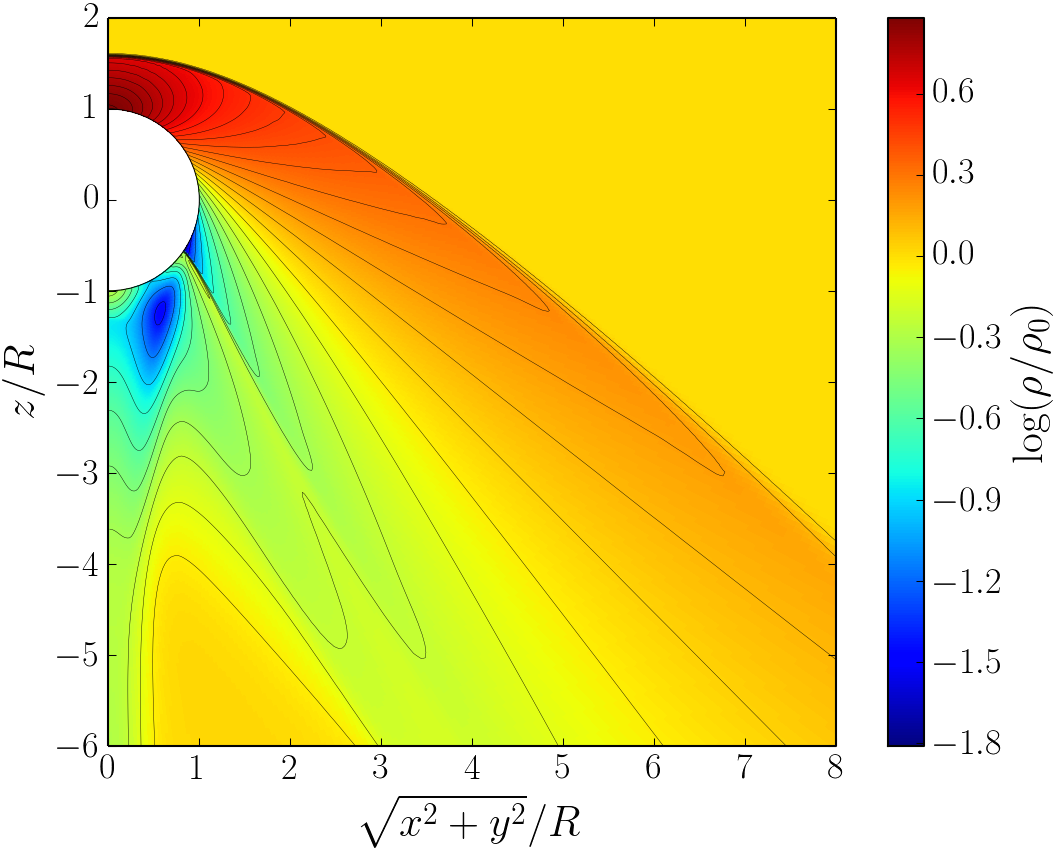
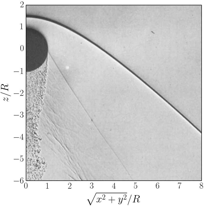
Figure 1: Visualization of a comparison simulation result of a sphere embedded in air ($\gamma=1.4$) flow at a Mach number $\mathcal{M}=1.53$. The homogeneous gas arrives from the top and flows in the negative $z$-direction. Shown is the density distribution for the final equilibrium state in the central part of the computational domain around the sphere.
Upper panel: Numerical results, black lines denote iso-density contours.
Bottom panel: Laboratory data from van Dyke (1982), Fig. 266.

4.1 Morphology

The black-and-white photography in van Dyke (1982), Fig. 266, displays the result of a laboratory experiment of a spherical non-gravitating body moving with supersonic velocity through air. We present the right half of the original image in Fig. 1, bottom panel. The morphology of the system is characterized by a standing shock front ahead of the moving sphere, a clearly visible shock boundary between the unperturbed and the perturbed gaseous medium, and a low-density region past the moving object.

We model the same experiment numerically within our framework described in the previous section. Here, we switch off the gravitational force of the moving body and use an adiabatic exponent for air of $\gamma=1.4$. The body is moving into the positive $z$-direction; actually, simulations are performed in the co-moving frame of the body, hence, the gas flow is initialized into the negative $z$-direction. The homogeneous gas is initialized with a constant density $\rho_{\infty}$. The Mach number of the flow is set to $\mathcal{M}=V_{\infty}/c_{\infty}=1.53$. In the whole computational domain the initial condition is given by the unperturbed flow. At the start of the simulation the rigid sphere is embedded and perturbs the flow. We run the model until an equilibrium state has been reached.

In Fig. 1, upper panel, we display the morphology of the gas density around the sphere in the numerical experiment. Clearly visible is the bow shock in front of the sphere, where the gas flow changes from supersonic to subsonic velocities, the shock front dividing the perturbed from the unperturbed gas, as well as the low-density region behind the moving body. As expected, the gas density reaches a maximum directly in front of the sphere. A visual comparison with the experimental data from van Dyke (1982), Fig. 266, as presented in Fig. 1, shows excellent agreement between the numerical experiment and the laboratory experiment in terms of their morphological characteristics. Furthermore, the magnitude of the density jump at the shock front from the numerical simulation agrees very well with the well-known analytical Rankine-Hugoniot jump conditions. In contrast to the axisymmetric and inviscid numerical result, the laboratory experiment shows that the low-density region past the moving object is subject to weak turbulence, that cannot be captured in the idealized simulation setting.

The following comparison checks for the shock front physics and its dependence on the Mach number.

4.2 The stand-off distance of the shock front

As we will point out later, the shock’s stand-off distance, $R_{\mathrm{SO}}$, plays a crucial role in determining the dynamical friction on a gravitating moving body. Here, we measure $R_{\mathrm{SO}}$ from the center of the moving spherical object. To test the dependence of the shock front on the problem’s Mach number, $\mathcal{M}$, we compute a sequence of models for the same setup as in the previous section but with a variety of different inflow velocities $V_{\infty}$. Fig. 2 shows the resulting stand-off distance of the shock, measured from the center of the sphere, as a function of $\mathcal{M}$.

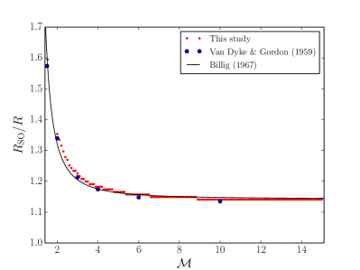
Figure 2: Quantitative comparison of the shock’s stand-off distance as function of Mach number. The solid black line denotes the relationship derived from laboratory experiments as given in the main text. Small red dots represent results from numerical experiments for the same setup. Blue dots denote early numerical results by van Dyke & Gordon (1959).

The $R_{\mathrm{SO}}$ decreases with increasing $\mathcal{M}$ and approaches asymptotically in the limit of highly supersonic flow a value of $R_{\mathrm{SO}}\rightarrow 1.14$. This outcome of the numerical experiments can be directly and quantitatively compared to the laboratory experiments by Billig (1967), using a derived fit to the laboratory data given by $R_{\mathrm{SO}}/R\simeq 1+0.143\exp\left(3.24/\mathcal{M}\right)$, where $R$ denotes the geometrical radius of the moving sphere. The results from the numerical and laboratory experiments are quantitatively in very good agreement, as shown in Fig. 2. They are consistent with each other at both extremes, weak shocks ($\mathcal{M}=1.53$) as well as strong shocks ($\mathcal{M}\rightarrow\infty$). In the regime of moderate shocks ($\mathcal{M}\sim 2\ldots 4$), the numerical experiments show slightly larger stand-off distances than the laboratory experiments. Additionally, in the numerical framework, the position of the shock front is associated with a certain grid cell, more specifically its center; no further interpolation has been applied. Hence, the visible steps in the numerical data visualize the finite spatial resolution of the numerical experiments.

4.3 The hydrodynamical drag force

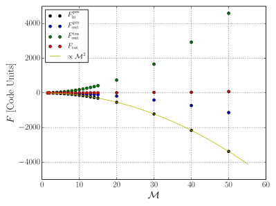
Figure 3: The force contributions in the equilibrium state according to Eq. (17) for the non-gravitating, rigid sphere in air, given as a function of the Mach number. $F^{\mathrm{prs}}_{\mathrm{in}}$ denotes the pressure force measured at the surface of the sphere, $F^{\mathrm{prs}}_{\mathrm{out}}$ the pressure force measured at the outer boundary of the computational domain, and $F^{\mathrm{trs}}_{\mathrm{out}}$ the momentum transport through the outer boundary. The sum of these three forces is denoted by $F_{\mathrm{tot}}$. The curve denotes a parabola with $F\propto\mathcal{M}^{2}$.

In Fig. 3 we display the contributions of the different forces acting on the gas and the sphere. Shown are the pressure force acting on the body, $F^{\mathrm{prs}}_{\mathrm{in}}$, together with the pressure and momentum flux at the outer boundary. As to be expected from Eq. (17) the sum of all 3 force contributions, $F_{\mathrm{tot}}$ adds up to zero. The error for the total force is slightly increasing for higher Mach numbers but is always below $2\%$ for all simulations. In this case the hydrodynamic drag acting on the body, given by $F^{\mathrm{prs}}_{\mathrm{in}}$, is negative which indicates a force opposing the direction of motion of the body. The standard drag force, as given in Eq. (5), depends quadratically on the velocity $V_{\infty}$ of the object. Our numerical results clearly confirm this expected quadratic scaling with $V_{\infty}$, see added solid line in Fig. 3.

5 Simulations of dynamical friction

#	$M$ [$\mbox{M}_{\mathrm{Jup}}$]	$R$ [$\mbox{R}_{\odot}$]	$\cal{M}$	$c_{\infty}$ [$\mbox{ km}\mbox{ s}^{-1}$]	$\gamma$	$R_{\mathrm{domain}}$ [$\mbox{R}_{\odot}$]	Figures
Fiducial simulation
F	60	0.01	4.0	58	5/3	10	Figs. 18 + 19
Fiducial simulation with larger domain size
C		0.01				25	Fig. 9
Variation of the mass of the perturber
M1	10 …  50	0.1					Fig. 8 + 16
M2	1 …120	0.01					Figs. 7 + 8 + 10 + 16
Variation of the velocity of the perturber
V1		0.1	3.5 …20.0	49	1.2		Fig. 12 + 13 + 15
V2		0.01	2.2 …10.9	53	1.4		Figs. 12 + 13 + 15 + 16
V3		0.1	2.0 …  9.0	58	5/3		Figs. 4 + 8 + 16
V4		0.01	2.0 …50.0	58	5/3		Figs. 5 + 7 + 8 + 11 + 12 + 13 + 15 + 16 + 17
V5		0.01	2.0 …20.0	63	2.0		Figs. 12 + 13 + 15 + 16
V6		0.1	2.0 …10.0	77	3.0		Figs. 12 + 13 + 15
V7		0.1	2.0 …10.0	89	4.0		Figs. 12 + 13 + 15
Variation of the soundspeed of the medium
S		0.01	1.6 …12.6	18.3 …183	5/3		Figs. 8 + 16
Variation of the adiabatic index of the medium
G		0.1	4.4	53	1.2 …6.0		Fig. 14 + 15

Table 1: Overview of series of simulations performed. Each row represents a series of individual simulations, mostly varying a single basic setup parameter. The columns denote from left to right the label of the simulation series, the mass, the radius, and the velocity of the perturber, the soundspeed of the gaseous medium, the adiabatic index of the medium, and the outer radius of the computational domain. The last column gives the figure numbers associated with the data processing of the simulation series. The body velocity is given in units of Mach. If the value of a parameter is not explicitly specified, the value from the fiducial simulation, given in the top row, is used.

Now we turn to astrophysical applications and consider the motion of a gravitating body through a homogeneous gaseous medium. For supersonic speeds a shock front ahead of the moving body is produced very similar to the morphology found in the laboratory experiments for the non-gravitating bodies. Fig. 4 shows the steady state solution for the gas mass density and the velocity field for one of our simulations. In front of the object a bow shock forms where the material is decelerated from supersonic to subsonic speeds. After passing the shock front, matter close to the object settles into a hydrostatic envelope. The major difference to the non-gravitating case is that behind the moving object a wake of higher-than-average density instead of lower density is formed, which is a direct consequence of the gravitational attraction of the body. In turn, this wake of higher density yields a gravitationally pull onto the object, which slows it down. This is the phenomenon of dynamical friction.

As shown above in Eq. (17) the total drag acting on a gravitating rigid body is the sum of the hydrodynamic drag (pressure force on the body, $F_{\mathrm{in}}^{\mathrm{prs}}$) and the dynamical friction, $F_{\mathrm{DF}}$. In our case, behind the shock front a spherical hydrostatic shell forms around the object such that the total pressure force on the object is negligible. Hence, the total drag on the object is given solely by dynamical friction, and in the following we shall concentrate on this part only, see Fig. 6 below. For very high Mach numbers the separation of the shock from the object’s surface becomes very small such that no hydrostatic envelope can form, and pressure effects will become important again.

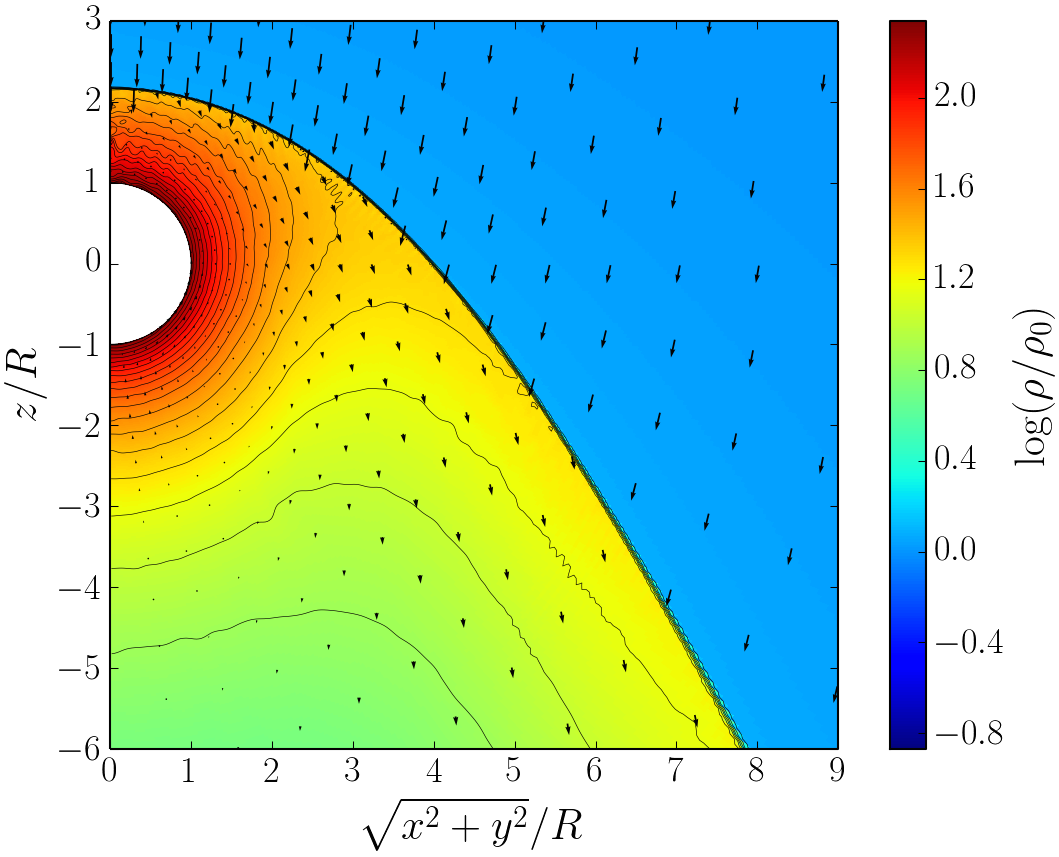
Figure 4: Density and velocity structure of the final quasi-stationary state around a gravitating object moving with supersonic motion through a gaseous homogeneous medium. The body is moving towards the positive $z$-direction. Density is color-coded and black lines denote iso-density contours. Velocities are given as arrows, scaled by the speed.

The dynamical friction of a body moving with supersonic speed through a gaseous homogeneous medium denotes a well defined problem, which involves a manageable amount of dependencies. In the course of this section, we first give an overview of the relevant problem parameters and how they are expected to impact the amount of dynamical friction (Sect. 5.1). Afterwards, we present our realized simulation series, each dedicated to investigate the impact of a specific parameter, and discuss the simulation results in terms of scaling laws (Sects. 5.5 to 5.7). Most importantly, the simulations’ outcome reveal the stand-off distance as the minimum spatial scale of the forming anisotropic density structure around the moving body. We analyze and discuss this new aspect in-depth and derive a semi-analytical relation between the stand-off distance and the accretion radius from fits to the numerical data in Sect. 5.3. Finally, we combine these findings to derive a convenient semi-analytical expression for the dynamical friction (Sect. 6).

We would like to point out again that we do not assume an a priori validity of the classic drag formula as stated in Eq. (1). Our procedure is to check the scaling of each parameter in Eq. (1) individually and confirm the existence of the logarithmic term. After this we demonstrate that the minimum distance $s_{min}$ in Eq. (2) is closely related to the stand-off distance of the shock from the object. We then present a new formula for calculating $s_{min}$ from the basic physical parameter of the problem.

5.1 The relevant problem parameters

First of all, the moving object is characterized by its mass $M$ and velocity $V_{\infty}$. The impact of these parameters on the dynamical friction is analyzed and discussed in Sects. 5.5 and 5.6. For high enough masses or small enough velocities, the smallest scale of interaction with the gas is set by the gravity of the moving object rather than its geometrical radius. In these cases, the moving body can also be treated as a point mass, as it is usually done in semi-analytical approaches, e.g. in the derivation by Ostriker (1999). Its geometrical radius $R$ becomes important for the interaction with the surrounding gas in cases of either low mass or high velocities, respectively. We investigate the impact of the geometrical radius in Sect. 5.3.

The gaseous homogeneous medium is characterized by two of the four quantities: mass density $\rho_{\infty}$, pressure $p_{\infty}$, temperature $T_{\infty}$, or soundspeed $c_{\infty}$. The remaining two are then determined according to Eqs. (12) and (13). In the following, we will choose the gas mass density $\rho_{\infty}$ and soundspeed $c_{\infty}$ as the independent variables; the mass density enters directly the force term of the gravitational pull of the wake onto the moving body and the soundspeed of the medium sets the Mach number ${\cal{M}}=V_{\infty}/c_{\infty}$ of the shock.

The thermodynamics of the gas is controlled by its caloric and thermal equations of state Eqs. (11) and (12) with the adiabatic index $\gamma$ as the only free parameter. Most important for the shock physics, the adiabatic index controls how the gaseous medium reacts in case of compression and expansion.

While the object is moving through the gaseous medium, a wake of higher density will form behind the object, which grows in time. For a known interaction time $t$, the extent of the wake is constrained by $s_{\mathrm{max}}=V_{\infty}t$. We discuss the dependence of the dynamical friction on the maximum extent of the wake in more detail in Sect. 5.4.

Summarized, the dynamical friction of a massive body moving supersonically through a gaseous homogeneous medium depends only on the mass of the body $M$, the velocity of the body $V_{\infty}$, its geometrical radius $R$, the mass density $\rho_{\infty}$ of the gas, its soundspeed $c_{\infty}$, the adiabatic index $\gamma$, and the maximum extent of the wake $s_{\mathrm{max}}$.

In Ruderman & Spiegel (1971), the authors give an expression for the dynamical friction as given in Eq. (1). In this formula, the dynamical friction depends additionally on the minimum length scale $s_{\mathrm{min}}$ of the interaction, a result of the spatial integration limits of the analytical derivation. From the analysis of the relevant parameters above, it follows that the parameter $s_{\mathrm{min}}$ is actually not a free parameter, but has to be a function of the parameters given above. In Sect. 5.3, we compute the minimum length scale of the interaction from our numerical solutions, associate this length scale with the shock’s stand-off distance, and derive its dependence on the relevant problem parameters.

In the following, we present the numerical experiments performed. The dependence of the dynamical friction on each of the relevant parameters is determined in a single or multiple dedicated simulation series. Table 1 gives an overview of the simulation series and their physical and numerical parameters. Due to the scale-freedom in the equations of the problem, the gas mass density can be chosen arbitrarily, we use a value of $\rho_{\infty}=1.510^{-4}\mbox{g cm}^{-3}$ in all simulations performed. In the table, the velocity of the body is giving in units of Mach. Simulations with varying soundspeed of the medium (series “S”) use the same velocity of the perturber, hence yield different Mach numbers as well. Simulations with varying adiabatic index of the medium (series “G”) use varying initial values of the gas pressure to keep the soundspeed the same in all simulations of the series.

5.2 The gas mass density

The dynamical friction should scale linearly with the density of the environment:

$$F_{\mathrm{DF}}\propto\rho_{\infty}$$ (18)

This scaling behavior is a direct consequence of the fact that the total dynamical friction is given by the sum of all the gravitational pulls from the environment onto the body. Each gravitational pull scales linearly with the density of the environment. Additionally, the hydrodynamical equations (see Sect. 3.2) are scale-free in density, and, hence, the flow morphology is independent on the initial density of the medium.

5.3 The minimum spatial scale of interaction

The total dynamical friction acting on the moving body is given by the spatial integral over the gravitational pull of the surrounding gaseous medium. According to Eqs. (1) and (2), it is expected to scale with the value of a minimum spatial interaction scale $s_{\mathrm{min}}$ according to the Coulomb logarithm:

$$F_{\mathrm{DF}}\propto\ln(s_{\mathrm{max}}/s_{\mathrm{min}})$$ (19)

Below this minimum interaction scale, the gaseous medium is assumed to exert no net gravitational pull on the body. What actually sets the minimum interaction scale is an open discussion in the literature.

5.3.1 A spatial force analysis

In our study, the approach of direct numerical experiments allows us to properly determine the minimum spatial interaction scale in case of gaseous media quantitatively. In order to derive the impact of each spatial scale individually, we first calculate the gravitational drag force acting on the object from the gas inside a specific shell at radius $r_{i}$ with a radial shell thickness of $r_{i+1/2}-r_{i-1/2}$:

$$\@vec{f}(r_{i})=-\int_{S(r_{i})}\,\frac{GM}{r^{2}}\leavevmode\nobreak\ \rho(\@vec{x})\leavevmode\nobreak\ \@vec{\hat{e}}_{r}\;\mathrm{d}V\,,$$ (20)

where the volume of shell $S(r_{i})$ is given by

$$S(r_{i})=2\pi\int_{0}^{\pi}\int_{r_{i-1/2}}^{r_{i+1/2}}\leavevmode\nobreak\ r^{2}\sin(\theta)\;\mathrm{d}r\;\mathrm{d}\theta\,.$$ (21)

The total gravitational force acting on the object is given by the sum over all shells:

$$\@vec{F}^{\mathrm{numerical}}_{\mathrm{DF}}=\sum_{i}\@vec{f}(r_{i})\,.$$ (22)

Even though the above Eq. (20) is written in vector form, only its $z$-component is non-zero due to the axial symmetry of the problem. The net gravitational drag will lead to a slow-down of the body, which is moving along the positive $z$-direction.

In Fig. 5, we show the fractions of the gravitational force $f(r_{i})$ as a function of radius or distance to the moving body, respectively.

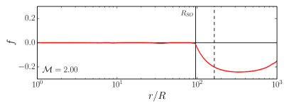
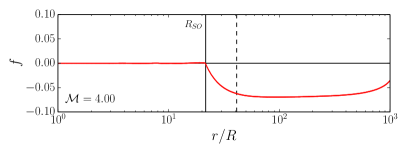
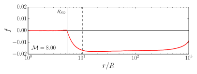
Figure 5: Fractions of the gravitational drag force $f(r_{i})$ to the total gravitational drag force acting on the moving object as a function of distance to the object. The vertical solid lines mark the stand-off distance $R_{\mathrm{SO}}$ of the shock ahead of the object, and the dashed vertical lines denote the accretion radius $R_{\mathrm{A}}$ according to Eq. (3). Results are shown for simulations with three different Mach numbers $\mathcal{M}$ as labeled in the bottom left corners.

The spatial analysis of the force is shown for three simulations with different Mach numbers of $\mathcal{M}=2,4,\mbox{ and }8$. Simulation parameters are given in Table 1, series “V4”.

The spatial analysis clearly reveals the so-called stand-off distance $R_{\mathrm{SO}}$ of the shock front as the searched-for minimum spatial interaction scale $s_{\mathrm{min}}$:

$$s_{\mathrm{min}}=R_{\mathrm{SO}}\,.$$ (23)

The associated bow shock forming in front of the body is visible in the density morphology depicted in Fig. 4. The shock front $R_{\mathrm{SO}}$ denotes the radius, where the flow changes from supersonic to subsonic velocities. Moreover, the density morphology around the body is characterized by the formation of a hydrostatic envelope extending up to $R_{\mathrm{SO}}$. This hydrostatic envelope is very close to spherical symmetry, as also depicted in Fig. 18. Hence, although this region marks the highest gas mass density, and in principle might have the strongest gravitational impact due to its closeness, the net gravitational pull within this hydrostatic envelope ($r<R_{\mathrm{SO}}$) turns out to be negligible. If at all, the stronger compression in the forward direction of the trajectory of the moving body yields a slight deviation from spherical symmetry, which actually results into a small gravitational acceleration instead of a drag. But this effect remains negligible compared to the total dynamical friction and is only marginally visible in Fig. 5 by eye for the case of highest Mach number; here, the fraction of the dynamical friction force close to but still below the stand-off distance has a positive sign, indicating positive acceleration of the body.

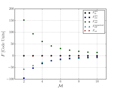
Figure 6: The force contributions for the equilibrium state according to Eq. (17) for the gravitating, rigid sphere, given as a function of the Mach number. $F^{\mathrm{prs}}_{\mathrm{in}}$ denotes the pressure force measured at the surface of the sphere, $F_{\mathrm{DF}}^{\mathrm{numerical}}$ denotes the total dynamical friction calculated according to Eq. (22), $F^{\mathrm{prs}}_{\mathrm{out}}$ the pressure force measured at the outer boundary of the computational domain, and $F^{\mathrm{trs}}_{\mathrm{out}}$ the momentum transport through the outer boundary. The sum of these 4 forces is denoted by $F_{\mathrm{tot}}$.

Clearly, the shells inside the sphere around the object with radius $R_{\mathrm{SO}}$ do not contribute to the total dynamical friction force, because around the object a spherically symmetrical hydrostatic envelope forms. This is confirmed in Fig. 6 where we plot the individual contributions to the total drag force on the spherical body, as a function of Mach number. As shown, the contribution of the pressure force, $F_{in}^{\mathrm{prs}}$, acting on the object is negligible. From this we can conclude that i) to calculate the drag acting on the object it is sufficient to consider the dynamical friction alone, and that ii) the relevant quantity for the minimum interaction scale $s_{\mathrm{min}}$ is given by $R_{\mathrm{SO}}$. Additional simulations with fixed Mach number $\mathcal{M}$ but different object masses $M$ give the same result for the spatial analysis of the force.

5.3.2 A convenient expression for the stand-off distance

It is the aim of this study to derive a general expression for the dynamical friction, that allows to compute the acting gravitational drag from the relevant problem parameters without the need of direct numerical simulations. As revealed in the previous section, such an expression for the dynamical friction will include a scaling with

$$F_{\mathrm{DF}}\propto\ln(s_{\mathrm{max}}/R_{\mathrm{SO}})\leavevmode\nobreak\ .$$ (24)

In the next step of our investigation, we derive an expression for the stand-off distance, which is based on the basic problem parameters only. Therefore, we make use of the apparent relationship of the stand-off distance $R_{\mathrm{SO}}$ to the accretion radius $R_{\mathrm{A}}$, see Eq. (3) for the definition of the accretion radius.

Fig. 5 seems to indicate that $R_{\mathrm{SO}}$ is directly proportional to the accretion radius $R_{\mathrm{A}}$. Since $R_{\mathrm{A}}$ scales as $\propto M/V_{\infty}^{2}$ we check these scaling laws for the stand-off distance as well. We use a series of simulations where we vary systematically the mass $M$ of the object and its velocity $V_{\infty}$. Simulation parameters are given in Table 1, series “M2” and “V4”. The results are displayed in Fig. 7.

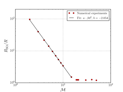
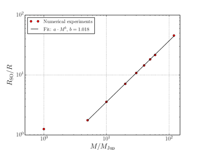
Figure 7: Correlation of the shock’s stand-off distance $R_{\mathrm{SO}}$ with object velocity or Mach number $\mathcal{M}$ respectively (top panel) and with object mass $M$ (bottom panel). Solid lines denote linear fits in the log-log plane.

Both panels show least-square fit lines that support the fact that $R_{\mathrm{SO}}\propto M/\mathcal{M}^{2}$. For larger $\mathcal{M}$ the stand-off distance becomes smaller according to $R_{\mathrm{SO}}\propto{\mathcal{M}^{-2}}$ as displayed in the top panel of Fig. 7. For fixed $\mathcal{M}$, lowering the object mass yields a smaller stand-off distance in agreement with $R_{\mathrm{SO}}\propto M$ as shown in the bottom panel of Fig. 7. This outcome confirms the scaling laws as long as the geometrical extent of the body $R$ is small compared to $R_{\mathrm{SO}}$. For high Mach shocks and for low body masses, respectively, the stand-off distance cannot decrease to smaller radii and approaches the size of the body $R$ instead. In all other cases, $R_{\mathrm{SO}}$ is directly proportional to $R_{\mathrm{A}}$:

$$R_{\mathrm{SO}}\propto R_{\mathrm{A}}\,.$$ (25)

An important difference between both radii is given by the fact that the stand-off distance depends on the thermodynamics of the system. As a consequence, we study the impact of the adiabatic index $\gamma$ on the stand-off distance and the final dynamical friction term in Sect. 5.7 below.

To investigate the proportionality between the two radii further, we perform additional simulations varying the mass, radius, and velocity of the object as well as the soundspeed of the medium. Detailed simulation parameters are given in Table 1. To find a useful general expression for the stand-off distance $R_{\mathrm{SO}}$ we utilize the non-linearity parameter

$$\eta=\frac{GM}{(\mathcal{M}^{2}-1)c_{\infty}^{2}R}=\frac{1}{2}\leavevmode\nobreak\ \frac{\mathcal{M}^{2}}{\mathcal{M}^{2}-1}\,\frac{R_{\mathrm{A}}}{R}\,,$$ (26)

as introduced by Kim & Kim (2009). In Fig. 8 we show the stand-off distance $R_{\mathrm{SO}}$ as well as the ratio of $R_{\mathrm{SO}}/R_{\mathrm{A}}$ as function of the non-linearity parameter $\eta$.

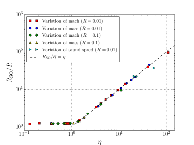
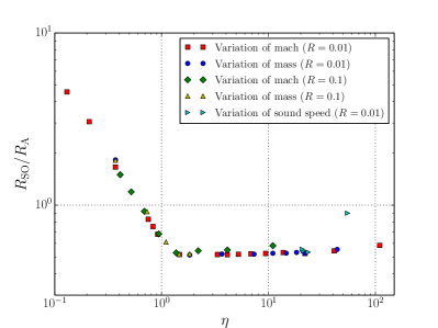
Figure 8: Correlation of the shock’s stand-off distance $R_{\mathrm{SO}}$ with the non-linearity parameter $\eta$, as given in Eq. (26), for various model sequences. In the top panel, $R_{\mathrm{SO}}$ is normalized by the object radius $R$. For $\eta>1$, a dashed line is superimposed, representing the relation $R_{\mathrm{SO}}/R=\eta$. In the bottom panel, $R_{\mathrm{SO}}$ is normalized by the corresponding accretion radius.

As seen in the top panel, for $\eta>1$ (larger $M$, lower $\mathcal{M}$) we find the scaling $R_{\mathrm{SO}}/R\propto\eta$, with an unknown proportional constant close to unity as indicated by the added dashed line. This is in good agreement with the results of Kim & Kim (2009). The largest deviation from this trend is seen in the rightmost green triangle, which belongs to a simulation in the weakly supersonic regime $\mathcal{M}=1.25$. A spatial analysis of the final configuration of this model shows that behind the shock front and around the object the gaseous medium is not in hydrostatic equilibrium – as for the supersonic cases – but displays small residual motions that did not disappear even in long-term runs. So, we expect deviations from the following relation (27) for non-supersonic flows, a regime that is not part of the present study and will have to be explored in future studies. For comparison, we denote that the rightmost red square belongs to a simulation with $\mathcal{M}=2$, but even larger $\eta$ than the green triangle run, and matches the found relationship much better.

For $\eta<1$ (larger $\mathcal{M}$, lower $M$) we enter the regime where the stand-off distance is limited by the size of the object $R$, and therefore the ratio $R_{\mathrm{SO}}/R$ remains constant. For this regime of low $\eta$, Kim & Kim (2009) find a different scaling due to the fact that they used a smoothed gravitational potential to model their perturber instead of the solid surface used in our study. Using the definition of $\eta$ (Eq. (26)), the proportionality $R_{\mathrm{SO}}/R\propto\eta$ implies

$$R_{\mathrm{SO}}\propto\frac{1}{2}\,\frac{\mathcal{M}^{2}}{\mathcal{M}^{2}-1}\leavevmode\nobreak\ R_{\mathrm{A}}\mbox{\leavevmode\nobreak\ \leavevmode\nobreak\ for }R_{\mathrm{SO}}\gg R\,.$$ (27)

Relation (27) represents a suitable expression for the stand-off distance. As pointed out above, the proportionality constant for the simulations performed so far seems to be very close to unity. But the relation still lacks the effect of different equations of state, i.e. any dependence on the adiabatic index $\gamma$. We investigate this dependence in detail in the following section.

The bottom panel of Fig. 8 just confirms for completeness again the proportionality between the stand-off distance and the accretion radius for different Mach numbers, object masses, and soundspeeds in the regime $R_{\mathrm{SO}}\gg R$. We checked in addition that a change in the size $R$ of the moving body does not influence the stand-off distance as long as $R$ remains substantially smaller than $R_{\mathrm{SO}}$. Hence, the curves for $R=0.1$ and $R=0.01$ are identical.

5.4 The maximum extent of the wake

The maximum extent of the wake past the body determines the size of the perturbed region, which will contribute to the total dynamical friction via its gravitational pull. In Eq. (1), the maximum extent of the wake enters as the outer radius of the integral $s_{\mathrm{max}}$ in the Coulomb-Logarithm $C_{A}$:

$$F_{\mathrm{DF}}\propto\ln({s_{\mathrm{max}}}/R_{\mathrm{SO}}).$$ (28)

For an infinite medium, the size of the wake $s_{\mathrm{max}}$ is given by the duration of the movement of the perturbing object. For a body starting its journey at $t=0$ with a constant velocity $V_{\infty}$, the time-dependent size of the wake $s_{\mathrm{max}}$ at a later time $t$ is given by the distance travelled $s_{\mathrm{max}}(t)=V_{\infty}t$.

The relation (28) implies that the dynamical friction increases as long as the body is moving through the medium, leading to a larger and larger wake. In principal, the dynamical friction seems to approach an infinitely high force for an infinitely long traveling object. In practice, the dynamical friction can not grow infinitely, even not for an infinitely large medium, because the dynamical friction acting on the body leads to a slow-down of the object on a dynamical timescale of the gas-body interaction (Sánchez-Salcedo & Brandenburg, 2001). The dynamical timescale of dynamical friction is given as the ratio of the initial momentum of the moving object and the acting force $t_{\mathrm{DF}}=MV_{\infty}/F_{\mathrm{DF}}$. Hence, the velocity of the perturber monotonically decreases in time until the body is at rest. As a consequence, the dynamical friction first increases (due to a growing extent of the wake) up to a maximum value and decreases afterwards (due to the slow-down of the body).

Here, we model the evolution of the system on timescales much smaller than the timescale for the slow-down of the body to extract the acting dynamical friction as a function of the relevant initial system parameters. As a next step, we check the scaling of the dynamical friction force with the extent of the wake. We compute the resulting dynamical friction by numerically integrating the gravitational pull of the forming wake onto the body up to different radii within the computational domain. As a result, we obtain the individual contributions of the wake at each radius. For further analysis, we extended the size of the computational domain to $R_{\mathrm{domain}}=25\mbox{R}_{\odot}$ (model C), other simulation parameter correspond to the fiducial case (model F) given in Table 1.

As shown in Fig.9, the scaling of the numerically determined drag force with the extent of the wake follows the expected logarithmic relation.

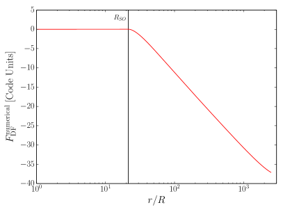
Figure 9: Scaling of dynamical friction with the size of the forming wake for model C in Table 1.

In the following, simulations make use of an arbitrary size of the computational domain, which just should be much larger than the stand-off distance of the shock. The finally acting dynamical friction can then be determined using the scaling relation Eq. (28). We use an outer radius of the computational domain of either $100\leavevmode\nobreak\ R$ or $1000\leavevmode\nobreak\ R$, depending on the specified radius $R$ of the moving body.

5.5 The mass of the perturber

The dimensional part of the dynamical friction formula – as written in Eqs. (1) and (5) – is expected to scale with the mass of the object squared:

$$F_{\mathrm{DF}}/C_{A}\propto M^{2}\,.$$ (29)

The physical explanation for this scaling relation is that the mass of the object first causes the accumulation of high density in the wake (a gravitational back-reaction, which scales linearly with the mass of the object), and secondly, the gravitational pull of the wake onto the object denotes a gravitational interaction, which again scales linearly with the mass of the object. But this argument is based on a linearization of the equations to relate the forming wake to a linear scaling with $M$.

Within our numerical framework, we can compute the total dependence of the dynamical friction on the mass, and can further check, if the dependence on $M$ can properly be split into a scaling with $M^{2}$ in the dimensional part and its further dependence within the dimensionless Coulomb logarithm $C_{A}$. We have performed numerical simulations for various masses $M$ of the perturber. Simulation parameters are given in Table 1, series “M2”. The resulting scaling of the ratio of dynamical friction and Coulomb logarithm is shown in Fig. 10.

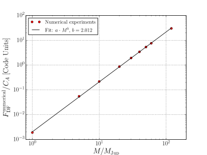
Figure 10: Correlation of the ratio of dynamical friction and Coulomb logarithm with the mass of the perturber.

The numerical experiments confirm the expected scaling very accurately.

5.6 The velocity of the perturber

The dimensional part of the dynamical friction formula – as written in Eqs. (1) and (5) – is expected to scale with the inverse of the velocity of the object squared:

$$F_{\mathrm{DF}}/C_{A}\propto V_{\infty}^{-2}$$ (30)

This scaling can only be true for supersonic motion and actually denotes a peculiarity of the dynamical friction, because usually hydrodynamical drag forces, as denoted in Eq. (5), scale with the square of the velocity, $V_{\infty}^{2}$. But in the case of dynamical friction, a faster body is already further away from the high-density wake, once it has formed. The distance of the body to the forming wake scales linearly with its velocity and the gravitational pull scales with the inverse of the distance squared.

As shown above, this inverse scaling with $V_{\infty}^{2}$ of the dynamical friction force, can be understood in terms of an effective cross section that is given by the accretion radius, $R_{\mathrm{acc}}$, that decreases with higher velocities of the body. This gives rise to the scaling of the dynamical friction with the inverse of the velocity of the object squared.

We have performed numerical simulations for various velocities $V_{\infty}$ of the perturber. Simulation parameters are given in Table 1, series “V4”. The resulting scaling of the ratio of dynamical friction and drag coefficient is shown in Fig. 11.

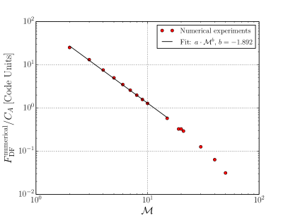
Figure 11: Correlation of the ratio of dynamical friction and Coulomb logarithm with the velocity of the perturber.

Again, the numerical experiments confirm the expected scaling. Deviations from the scaling law occur for very high Mach numbers, because the stand-off distance cannot shrink to arbitrarily small values and approaches the geometrical radius of the body instead, cp. discussion in Sect. 5.3 for details, especially Fig. 7.

5.7 The adiabatic index

All the simulations presented in the previous sections use an adiabatic index of $\gamma=5/3$. This was also the one and only value for the adiabatic index investigated in Kim & Kim (2009). But in fact, the compression in the shocked region around the object as well as the compression in the wake behind the moving body depends on the equation of state in use, and hence, on the value of the adiabatic index. In an extreme case, for very large values of the adiabatic index, the gaseous medium becomes incompressible for example, because any compression (increase in density) causes the pressure to increase infinitely strong, which causes an infinitely strong pressure force, and the medium directly relaxes towards an iso-density morphology again.

To further investigate the generality of our results so far we perform a variety of additional model sequences using different adiabatic indices. Detailed setup parameters of these simulation series are given in Table 1.

The correlation of the stand-off distance with the velocity of the perturber is shown in Fig. 12, but now for a variety of different values of the adiabatic index $\gamma$.

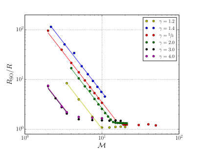
Figure 12: Correlation of the shock’s stand-off distance with the Mach number for different values of the adiabatic index $\gamma$. Dots denote results from the numerical simulations. The colored lines represent the scaling of $R_{\mathrm{SO}}/R\propto\mathcal{M}^{-2}$.

For large Mach numbers $\mathcal{M}$, the stand-off distance approaches the geometrical radius of the object. For lower $\mathcal{M}$, as indicated by the colored lines, all simulation series confirm the scaling law of $R_{\mathrm{SO}}/R\propto\mathcal{M}^{-2}$ as previously determined in Fig. 7.

In Fig. 13 top panel, the correlation of the stand-off distance with the non-linearity parameter $\eta$ is shown for different values of $\gamma$.

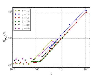
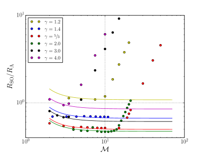
Figure 13: Correlation of the shock’s stand-off distance with the non-linearity parameter $\eta$ given in Eq. (26) (top panel) and the Mach number (bottom panel). The top panel is analogous to the top panel of Fig. 8, but now with results for different values of the adiabatic index $\gamma$. Dots denote results from the numerical simulations. Colored lines represent the relations discussed in the main text.

Colored lines indicate linear fits in the log-log plane of the plot. Since we found $R_{\mathrm{SO}}/R\propto\eta$ for $\gamma=\nicefrac{{5}}{{3}}$ in agreement with Kim & Kim (2009), we assume the following, more general relation:

$$\frac{R_{\mathrm{SO}}}{R}=g(\gamma)\,\eta\,,$$ (31)

where the factor $g(\gamma)$ describes the dependence on the adiabatic index $\gamma$. Specific values of this function are obtained according to the linear fits to the numerical experiments, namely

$\gamma$	1.2	1.4	5/3	2.0	3.0	4.0
$g(\gamma$)	2.17	1.33	1.00	0.95	1.22	1.70

For large values of the adiabatic index, namely $\gamma=3$ and $4$, the accuracy of the fit values has to be taken with care, because the fits rely on three to four data points only.

In the bottom panel of Fig. 13, the stand-off distance is shown in units of the accretion radius as a function of the Mach number. Also here, the previously determined correlation between the stand-off distance and the accretion radius (Eq. (27)) can be generalized to include the dependence on the adiabatic index $\gamma$ via:

$$R_{\mathrm{SO}}=\frac{g(\gamma)}{2}\,\frac{\mathcal{M}^{2}}{\mathcal{M}^{2}-1}\,R_{\mathrm{A}}\,.$$ (32)

This function is presented as colored lines in the bottom panel of Fig. 13. Values for $g(\gamma)$ were used as given above.

In appendix B, we derive an analytical estimate of the $\gamma$-dependence of the stand-off distance:

$$\frac{R_{\mathrm{SO}}}{R_{\mathrm{A}}}\lesssim\frac{((\gamma)+1)^{2}}{4(\gamma)}\left[1-\left(\frac{((\gamma)-1)}{(\gamma)+1}\right)^{(\gamma)-1}\right]^{-1}-1$$ (33)

This relation is shown in comparison to a simulation series of varying adiabatic index in Fig. 14.

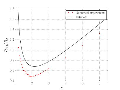
Figure 14: Stand-off distance in units of accretion radius $R_{\mathrm{SO}}/R_{\mathrm{A}}$ as a function of the adiabatic index $\gamma$. The black line denotes the analytically estimated upper limit given in Eq. (33).

The estimate does not allow for an exact determination, but it denotes an upper limit of the stand-off distance. Most importantly, the estimate follows the trend of the $\gamma$-dependence when compared to the numerical experiments.

Due to the similarity to the $\gamma$-dependence, we choose the analytical estimate as the basis function of a fit to the numerical data, but allow now for a shift in $\gamma\rightarrow\gamma+a$ and in $R_{\mathrm{SO}}/R_{\mathrm{A}}\rightarrow R_{\mathrm{SO}}/R_{\mathrm{A}}+b$:

$$\frac{R_{\mathrm{SO}}}{R_{\mathrm{A}}}\approx\frac{((\gamma+a)+1)^{2}}{4(\gamma+a)}\left[1-\left(\frac{((\gamma+a)-1)}{(\gamma+a)+1}\right)^{(\gamma+a)-1}\right]^{-1}-1-b$$ (34)

with $a$ and $b$ as free fitting parameters. A least square fit of this function to the numerical data yields $a=0.1$ and $b=0.18$.

Using Eq. (32) for the $\mathcal{M}=4.0$ numerical data in combination with the fitted function Eq. (34) allows to give an approximate function of $g(\gamma)$:

$$g(\gamma)\approx\frac{15}{8}\left\{\frac{((\gamma+a)+1)^{2}}{4(\gamma+a)}\left[1-\left(\frac{((\gamma+a)-1)}{(\gamma+a)+1}\right)^{(\gamma+a)-1}\right]^{-1}\negthickspace-1-b\right\}$$ (35)

with $a=0.1$ and $b=0.18$.

As a further check of the approximate function, we can compare this relation with the tabular values above derived via Eq. (31), see Fig. 15.

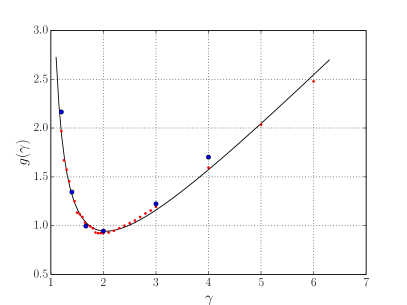
Figure 15: Comparison of the semi-analytical approximation of the function $g(\gamma)$, see Eq (35), shown as a black line with numerically obtained values. Small red dots denote the simulation series “G” with varying adiabatic index; each red dot represents a single simulation. Larger blue dots denote values derived by fitting the scaling of the stand-off distance with the non-linearity parameter for a variety of different simulation series shown in the top panel of Fig. 13; each blue dot represents such a fit value to a full simulation series. See main text for details of the derivation.

The approximate function $g(\gamma)$ for the overall $\gamma$-dependence gives reasonable results in comparison to the numerical outcome. As stated previously, for large values of the adiabatic index, namely $\gamma=3$ and $4$, the accuracy of the fit values (big blue dots) has to be taken with care, because the fits rely on three to four data points only.

6 A new formula of dynamical friction

As a final step, we combine our obtained scaling law for the stand-off distance, $R_{\mathrm{SO}}$, and the dependence on the adiabatic index, $\gamma$, to formulate a new general expression for the dynamical friction of a gravitating body of mass $M$ and radius $R$ moving supersonically with velocity $V_{\infty}$ through a homogeneous gaseous medium of mass density $\rho_{\infty}$ and soundspeed $c_{\infty}$:

$$F_{\mathrm{DF}}=4\pi\rho_{\infty}\left(\frac{GM}{V_{\infty}}\right)^{2}\leavevmode\nobreak\ \ln\left(\frac{s_{\mathrm{max}}}{R_{\mathrm{SO}}}\right).$$ (36)

The determination of the drag force from the basic problem parameters only requires an a priori knowledge of the stand-off distance. As shown above, the shock’s stand-off distance $R_{\mathrm{SO}}$ can be approximated by

$$R_{\mathrm{SO}}=\frac{g(\gamma)}{2}\leavevmode\nobreak\ \frac{\mathcal{M}^{2}}{\mathcal{M}^{2}-1}\leavevmode\nobreak\ R_{\mathrm{A}},$$ (37)

with $g(\gamma)$ given by Eq. (35).

Strictly speaking, the formula above for the stand-off distance is only valid for a stand-off distance larger than the geometrical radius of the object. In the regime of large, low-mass bodies moving with high velocity, the stand-off distance approaches the value of the geometrical radius instead, and one can replace $s_{\mathrm{min}}$ by the object size $R$.

We check the overall accuracy of this approximate determination of dynamical friction in direct comparison to the various numerical experiments performed herein, covering a broad parameter space in terms of the dimensionless non-linearity parameter $\eta=[2\leavevmode\nobreak\ (\mathcal{M}^{2}-1)/\mathcal{M}^{2}\leavevmode\nobreak\ R/R_{\mathrm{A}}]^{-1}$. The result of this comparison is shown as the ratio of the force in the experiments and the approximate formula in Fig. 16.

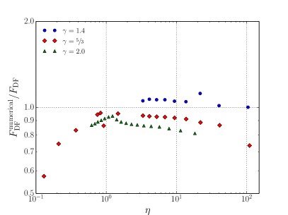
Figure 16: Comparison of the newly derived approximate formula for dynamical friction $F_{\mathrm{DF}}$ with data from various numerical experiments $F^{\mathrm{numerical}}_{\mathrm{DF}}$. The corresponding ratio is given as function of the non-linearity parameter $\eta$. Top panel shows results from a variety of simulations with adiabatic index $\gamma=5/3$, varying the Mach number, soundspeed, and object mass. Bottom panel shows results from a variety of simulations with varying Mach number for different adiabatic indices as labeled.

The approximate formula can be used as a convenient tool to estimate the drag force from the basic parameters in reasonable accuracy. Especially in the regime of $1\leq\eta\leq 50$ the estimated values match the numerical experiments. Largest deviations are observed in the marginally supersonic regime ($\mathcal{M}$ close to unity, denoted by the rightmost greenish triangle) and in cases, where the shock’s stand-off distance approaches the size of the object. The latter effect is visible when comparing the numerical outcome in the regime of large $\eta$ for simulations with a larger (green diamonds) and smaller object radii (red squares) in the top panel of Fig. 16.

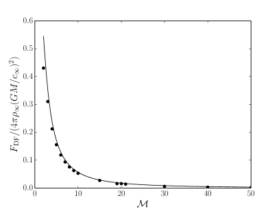
Figure 17: The normalized drag force as a function of the Mach number. The solid line resembles our newly derived formula as given in Eq. (36). The numerical data are given by the black dots, for which we we used simulation series V4.

To compare how well our newly derived formula approximates the drag force, $F_{\mathrm{DF}}$, we plot in Fig. 17 the numerically calculated drag force divided by the factor $4\pi\rho_{\infty}\left(GM/c_{\infty}\right)^{2}$ for varying Mach numbers of the perturber as black dots. The relation

$$F_{\mathrm{DF}}/(4\pi\rho_{\infty}\left(GM/c_{\infty}\right)^{2})=C_{A}/\mathcal{M}^{2}$$ (38)

is shown as solid black line, where we use $C_{A}=\ln(s_{\mathrm{max}}/R_{\mathrm{SO}})$ with $R_{\mathrm{SO}}$ according to equation (32). For the maximum radius in $C_{A}$ we used $r_{max}=1000R$. As seen our approximative function for $C_{A}$ reflects the numerical data very well.

7 Summary

We derived a new formula for dynamical friction of a body moving with supersonic speed through a homogeneous gaseous medium. This formula was obtained by following an ansatz of direct numerical modeling of the dynamical problem.

In 11 simulation series, including slightly more than 100 individual simulations in total, we scanned the parameter space of the problem and derived the scaling relations of the dynamical friction with the mass, the velocity, and radius of the moving body, the gas mass density, its soundspeed, and the value of the adiabatic index, as well as the maximum extent of the forming wake.

7.1 Scaling relations

As expected, the dimensional part of the dynamical friction formula as given in Eq. (36) scales proportional to the mass of the moving body squared, and to the inverse of its velocity squared. Furthermore, the dynamical friction $F_{\mathrm{DF}}$ scales linearly with the gas mass density and is proportional to the logarithm of the ratio of the spatial extents of the forming wake and the shock’s stand-off distance.

7.2 The minimum spatial interaction scale

The numerical experiments allow us to not only compute the total dynamical friction acting on the body, but also to investigate the individual contributions to the dynamical friction induced as a function of the distance to the perturber. The outcome of this analysis reveals that the region within the stand-off distance $R_{\mathrm{SO}}$ of the shock does not contribute to the dynamical friction of a gaseous medium (see Fig. 5 and associated main text for details). At radii smaller than the stand-off distance, a spherically symmetric stratified atmosphere forms around the moving body, which due to its symmetry induces no net gravitational pull or pressure force. Only at radii above the stand-off distance, a wake of higher density forms behind the moving body and induces a gravitational drag force.

Hence, in the well-known formulae by Ruderman & Spiegel (1971) or Ostriker (1999), it is the stand-off distance $R_{\mathrm{SO}}$ of the shock, which determines the minimum length scale $s_{\mathrm{min}}$ required in the so-called Coulomb-Logarithm $C_{A}=\ln(s_{\mathrm{max}}/s_{\mathrm{min}})$:

$$s_{\mathrm{min}}=R_{\mathrm{SO}}\leavevmode\nobreak\ .$$ (39)

The formation of a spherically symmetric atmosphere (with radius $R_{\mathrm{SO}}$) around a gravitating object implies that the hydrodynamical drag force vanishes in contrast to the non-gravitating case. But for very high Mach numbers the shock moves very close to the object so that $R_{\mathrm{SO}}\approx R$. In this case no spherically symmetric envelope around the object formes and the hydrodynamical drag becomes important again.

7.3 Relating the stand-off distance to the accretion radius

In a second step, to allow an easy computation of the stand-off distance for general dynamical friction problems, we derived the relation of the shock’s stand-off distance to the common definition of the accretion radius:

$$R_{\mathrm{A}}=\frac{2GM}{V_{\infty}^{2}}\leavevmode\nobreak\ ,$$ (40)

depending only on the mass $M$ and velocity $V_{\infty}$ of the perturber. The stand-off distance is directly proportional to the accretion radius and the proportionality constant depends on the Mach number and the adiabatic index of the gas only.

$$R_{\mathrm{SO}}=\frac{g(\gamma)}{2}\,\frac{\mathcal{M}^{2}}{\mathcal{M}^{2}-1}\leavevmode\nobreak\ R_{\mathrm{A}}\leavevmode\nobreak\ .$$ (41)

Additionally, the geometrical radius $R$ of the moving body yields a lower limit for the stand-off distance $(R_{\mathrm{SO}}\geq R)$.

Via an analytical estimate of the stand-off distance and further fitting of the remaining free parameters, we gave an approximate relation of the dependence of the shock’s stand-off distance on the adiabatic index $\gamma$ of the gaseous medium:

$$g(\gamma)=\frac{15}{8}\left\{\frac{(\gamma^{\prime}+1)^{2}}{4\gamma^{\prime}}\left[1-\left(\frac{(\gamma^{\prime}-1)}{\gamma^{\prime}+1}\right)^{\gamma^{\prime}-1}\right]^{-1}-1-b\right\}$$ (42)

with $\gamma^{\prime}=\gamma+a$ and values of $a=0.1$ and $b=0.18$.

7.4 An updated formula of dynamical friction

Finally, we combined the derived scaling relations and the finding on the stand-off distance to give an update of the well-known formula of dynamical friction acting on a body of mass $M$ moving at supersonic speed $V_{\infty}$ through a gaseous homogeneous medium of mass density $\rho_{\infty}$:

$$F_{\mathrm{DF}}=4\pi\rho_{\infty}\left(\frac{GM}{V_{\infty}}\right)^{2}\leavevmode\nobreak\ \ln\left(\frac{s_{\mathrm{max}}}{R_{\mathrm{SO}}}\right)\leavevmode\nobreak\ ,$$ (43)

where $s_{\mathrm{max}}$ denotes the extent of the wake and $R_{\mathrm{SO}}$ can be obtained using the derived formulae above.

Appendix A Hydrostatic equilibrium stratification

As mentioned in the text, behind the shock front and around the object the material is very subsonic and can be approximated by assuming a hydrostatic equilibrium. The morphology is illustrated in more detail in Fig. 18 where we show the stratification of different physical quantities in different directions. The data shown is extracted from a simulation with the fiducial parameters as specified in Table 1.

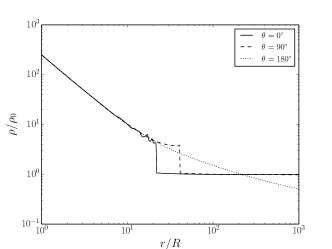
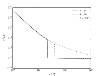
Figure 18: Stratification around the moving object. Values in front of the moving object ($\theta=0$), perpendicular to its velocity ($\theta=90$), and behind the object ($\theta=180$) are displayed. From top to bottom, the panels show gas density, pressure, Mach number, and entropy of the flow.

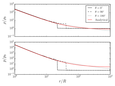
Figure 19: Stratification of gas density (upper panel) and pressure (bottom panel) around the moving object. As in the previous figure, values in front of the moving object ($\theta=0$), perpendicular to its velocity ($\theta=90$), and behind the object ($\theta=180$) are displayed. The additional red lines denote the analytical estimates obtained from Eqs. (50) and (45), respectively. In the formula of the estimate, a value for the stand-off distance of $x_{\mathrm{SO}}=0.533$ was used, in accordance with the final quasi-stationary state of the numerical experiment.

As clearly visible, within the stand-off radius, as given by the discontinuity of the solid curve, all three cuts agree with each other, and hence the stratification is spherically symmetric. Because of the Mach number being very close to zero it is hydrostatic as well. Here, we derive analytical relations for this stratification that will be used in the following section of the appendix to obtain an analytical estimate on the shock’s stand-off distance.

For spherical symmetry the equation of hydrostatic equilibrium reads

$$\frac{1}{\rho}\frac{dp}{dr}=-\frac{d\phi}{dr}$$ (44)

where $\phi$ is the gravitational potential. Now we use an adiabatic approximation for the pressure

$$p=K\rho^{\gamma}\,,$$ (45)

where $K$ is a constant, and integrate from a reference radius $r_{0}$ to $r$, yielding:

$$\left(\frac{\rho}{\rho_{0}}\right)^{\gamma-1}=1-\frac{\gamma-1}{c_{0}^{2}}\,\left(\phi(r)-\phi_{0}\right).$$ (46)

Here the subscript $0$ refers to the reference radius $r_{0}$ where the values are known.

As a next step, we want to analyze the bow-shock in front of the object. We can find the physical properties behind the shock from the standard jump conditions

$$\frac{\rho_{2}}{\rho_{1}} =\frac{(\gamma+1)\mathcal{M}_{1}^{2}}{(\gamma-1)\mathcal{M}_{1}^{2}+2}$$ (47)

$$\frac{p_{2}}{p_{1}} =\frac{(\gamma+1)+2\gamma(\mathcal{M}_{1}^{2}-1)}{\gamma+1}$$ (48)

Here, the index ’1’ refers to the pre-shock values (supersonic regime) and the index ’2’ to the post-shock (subsonic) regime. These are valid in a reference frame moving with the shock. In our case the shock is stationary in the co-moving frame of the body, and we can directly apply the jump conditions, knowing the pre-conditions. The simulations show that for the density, pressure, and temperature the pre-shock values, at the the stand-off radius $R_{\mathrm{SO}}$, are just the prescribed inflow values (at $\infty$), compare also Fig. 18.

To obtain the pre-shock Mach-number $\mathcal{M}_{1}$ at this radius we use the free-fall condition. From the conservation of energy (kinetic and gravitational), we obtain

$$\mathcal{M}_{1}=\mathcal{M}_{\infty}\,\left(1+\frac{1}{x_{SO}}\right)^{1/2}$$ (49)

where the coordinate $x$ denotes the radial distance to the shock front in units of the accretion radius, specifically $x_{\mathrm{SO}}=R_{\mathrm{SO}}/R_{\mathrm{A}}$. Eq. (49) matches the simulation outcome quite well, cp. Fig. 18.

To obtain the (hydrostatic) post-shock density stratification around the object we first use these normalizations to obtain the general relation

$$\rho(x)=\rho_{0}\left[1-\frac{\gamma-1}{c_{0}^{2}/c_{\infty}^{2}}\frac{\mathcal{M}_{\infty}^{2}}{2}\left(\frac{1}{x_{0}}-\frac{1}{x}\right)\right]^{1/\gamma-1}$$ (50)

with an arbitrary point $x_{0}$ where $\rho_{0}$ and $c_{0}$ are known values at the reference radius. If we choose now $x_{0}=x_{\mathrm{SO}}$, the other quantities correspond to the desired postshock quantities and can be obtained from the jump conditions, using $\mathcal{M}_{1}$ from Eq. (49). The required shock-position $x_{\mathrm{SO}}$ enters at this point as a free parameter, obtained from the numerical solution.

Appendix B An estimate for the stand-off distance

Because the stratification around the object is nearly hydrostatic, one can obtain some limits on $x_{\mathrm{SO}}$. Here, we use the strong shock conditions, i.e. $\mathcal{M}_{1}\rightarrow\infty$ and obtain for the jumps in density and pressure

$$f_{\rho}\equiv\frac{\rho_{2}}{\rho_{1}} =\frac{\gamma+1}{\gamma-1}$$ (51)

$$f_{p}\equiv\frac{p_{2}}{p_{1}} =\frac{2\gamma\mathcal{M}_{1}^{2}}{\gamma+1}$$ (52)

and hence for the post-shock soundspeed (in units of $c_{\infty}$)

$$c_{\mathrm{SO}}^{2}=\frac{f_{p}}{f_{\rho}}=\frac{2\gamma\mathcal{M}_{1}^{2}}{(\gamma+1)^{2}}\,(\gamma-1)\,.$$ (53)

Now, we assume that for large distances, $x\rightarrow\infty$, the density of the post-shock stratification lies below the unperturbed density $\rho(x\rightarrow\infty)\leq\rho_{\infty}$ as seen in the simulations. This fact is displayed in Fig. 19 where the analytical post-shock stratification (red solid curve) lies for large radii just below the unperturbed value $\rho_{\infty}$. Inserting Eq. (53) in Eq. (50) yields

$$1\geq\frac{\gamma+1}{\gamma-1}\,\left[1-\frac{(\gamma+1)^{2}\mathcal{M}_{\infty}^{2}}{2\gamma\mathcal{M}_{1}^{2}2}\frac{1}{x_{\mathrm{SO}}}\right]^{1/\gamma-1}$$ (54)

with $\mathcal{M}_{1}$ from Eq. (49). Solving for $x_{\mathrm{SO}}$ finally leads to

$$x_{\mathrm{so}}\leq\frac{(\gamma+1)^{2}}{4\gamma}\,\left[1-\left(\frac{\gamma-1}{\gamma+1}\right)^{\gamma-1}\right]^{-1}-1\,.$$ (55)

This function is shown in Fig. 14 in comparison to data from numerical simulations. While the relation (55) cannot give the exact value for $R_{\mathrm{SO}}$ it nevertheless provides a reasonable upper limit for the stand-off distance, and follows the trend of the obtained numerical results.

Appendix C Convergence study

We ran simulations using varying grid sizes from roughly $10^{3}$ up to $10^{6}$ grid cells in total (more precisely, we varied the number of grid cells from $N_{\mathrm{r}}\times N_{\mathrm{\theta}}=50\times 23=1150$ up to $N_{\mathrm{r}}\times N_{\mathrm{\theta}}=1720\times 790=1.3588\times 10^{6}$ grid cells). The inner radial boundary of these simulations was chosen to $R=0.01\mbox{ R}_{\odot}$. Other simulation parameters correspond to the “fiducial setup” given in Table 1. From the final quasi-stationary state, we determine the two most relevant physical quantities of our investigation, namely the shock’s stand-off distance $R_{\mathrm{SO}}$ and the dynamical friction $F^{\mathrm{numerical}}_{\mathrm{DF}}$ acting on the moving body.

Results of this convergence study are presented in Fig. 20.

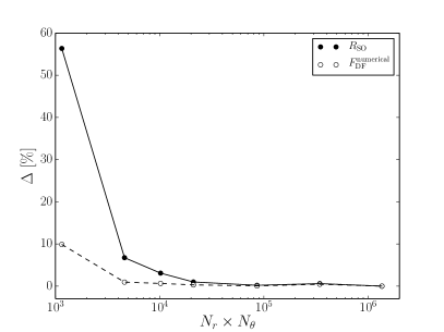
Figure 20: Convergence test of the numerical setup. Values on the horizontal axis denote the total number of grid cells $N_{\mathrm{r}}\times N_{\mathrm{\theta}}$. The vertical axis shows the relative deviation of the resulting stand-off distance $R_{\mathrm{SO}}$ (solid circles) and the dynamical friction $F^{\mathrm{numerical}}_{\mathrm{DF}}$ (dashed circles) from its corresponding value of the highest resolution run.

Deviations are given as relative differences to the values from the highest resolution simulation using more than $10^{6}$ grid cells. The numerical results show a clear convergence trend. For numerical grids larger than $10^{5}$ grid cells, the deviations become negligibly small. To be on the very safe side, we chose $N_{\mathrm{r}}\times N_{\mathrm{\theta}}=860\times 400=3.44\times 10^{5}$ grid cells as our default resolution for the simulations performed. Simulations with a larger inner radial boundary of $R=0.1\mbox{ R}_{\odot}$ require less grid cells in the radial direction, especially due to the logarithmic grid in the radial direction. Nonetheless, we also use here a comparable grid size of $N_{\mathrm{r}}\times N_{\mathrm{\theta}}=700\times 480=3.36\times 10^{5}$ grid cells as our default resolution.