Reachability Oracles for Directed Transmission Graphs

Abstract

Let $P\subset\mathbb{R}^{d}$ be a set of $n$ points in $d$ dimensions such that each point $p\in P$ has an associated radius $r_{p}>0$. The transmission graph $G$ for $P$ is the directed graph with vertex set $P$ such that there is an edge from $p$ to $q$ if and only if $|pq|\leq r_{p}$, for any $p,q\in P$.

A reachability oracle is a data structure that decides for any two vertices $p,q\in G$ whether $G$ has a path from $p$ to $q$. The quality of the oracle is measured by the space requirement $S(n)$, the query time $Q(n)$, and the preprocessing time. For transmission graphs of one-dimensional point sets, we can construct in $O(n\log n)$ time an oracle with $Q(n)=O(1)$ and $S(n)=O(n)$. For planar point sets, the ratio $\Psi$ between the largest and the smallest associated radius turns out to be an important parameter. We present three data structures whose quality depends on $\Psi$: the first works only for $\Psi<\sqrt{3}$ and achieves $Q(n)=O(1)$ with $S(n)=O(n)$ and preprocessing time $O(n\log n)$; the second data structure gives $Q(n)=O(\Psi^{3}\sqrt{n})$ and $S(n)=O(\Psi^{3}n^{3/2})$; the third data structure is randomized with $Q(n)=O(n^{2/3}\log^{1/3}\Psi\log^{2/3}n)$ and $S(n)=O(n^{5/3}\log^{1/3}\Psi\log^{2/3}n)$ and answers queries correctly with high probability.

1 Introduction

Representing the connectivity of a graph in a space efficient, succinct manner, while supporting fast queries, is one of the most fundamental data structure questions on graphs. For an undirected graph, it suffices to compute the connected components and to store with each vertex a label for the respective component. This leads to a linear-space data structure that can decide in constant time if any two given vertices are connected. For directed graphs, however, connectivity is not a symmetric relation any more, and the problem turns out to be much more challenging. Thus, if $G$ is a directed graph, we say that a vertex $s$ can reach a vertex $t$ if there is a directed path in $G$ from $s$ to $t$. Our goal is to construct a reachability oracle, a space efficient data structure that answers reachability queries, i.e., that determines for any pair of query vertices $s$ and $t$ whether $s$ can reach $t$. The quality of a reachability oracle for a graph with $n$ vertices is measured by three parameters: the space $S(n)$, the query time $Q(n)$ and the preprocessing time. The simplest solution stores for each pair of vertices whether they can reach each other, leading to a reachability oracle with $\Theta(n^{2})$ space and constant query time. For sparse graphs with $O(n)$ edges, storing just the graph and performing a breadth first search for a query yields an $O(n)$ space oracle with $O(n)$ query time. Interestingly, other than that, we are not aware of any better solutions for general directed graphs, even sparse ones; see Cohen et al. [5] for partial results. Thus, any result that simultaneously achieves subquadratic space and sublinear query time would be of great interest. A lower bound by Pǎtraşcu [12] shows that we cannot hope for $o(\log n)$ query time with $O(n)$ space in sparse graphs, but it does not rule out constant time queries with slightly superlinear space. In the absence of progress towards non-trivial reachability oracles or better lower bounds, solutions for special cases become important. For directed planar graphs, after a long line of research [2, 7, 6, 4, 13], Holm, Rotenberg and Thorup presented a reachability oracle with constant query time and $O(n)$ preprocessing time and space usage [8]. This data structure, as well as most other previous reachability oracles, can also return the approximate shortest path distance between the query vertices.

Transmission graphs constitute a graph class that shares many similarities with planar graphs: let $P\subset\mathbb{R}^{2}$ be a set of points where each point $p\in P$ has a (transmission) radius $r_{p}$ associated with it. The transmission graph has vertex set $P$ and a directed edge between two distinct points $p,q\in P$ if and only if $|pq|\leq r_{p}$, where $|pq|$ denotes the Euclidean distance between $p$ and $q$. Transmission graphs are a common model for directed sensor networks [10, 11, 14]. In this geometric context, it is natural to consider a more general type of query where the target point is an arbitrary point in the plane rather than a vertex of the graph. In this case, a vertex $s\in P$ can reach a point $q\in\mathbb{R}^{2}$ if there is a vertex $t\in P$ such that $s$ reaches $t$ and such that $|tq|\leq r_{t}$. We call such queries geometric reachability queries and we call oracles that can answer such queries geometric reachability oracles. To avoid ambiguities, we sometimes use the term standard reachability query/oracle when referring to the case where the query consists of two vertices.

Our Results.

An extended abstract of this work was presented at the 31st International Symposium on Computational Geometry [9]. This abstract also discusses the problem of constructing sparse spanners for transmission graphs. While we were preparing the journal version, it turned out that a full description of our results would yield a large and unwieldy manuscript. Therefore, we decided to split our study on transmission graphs into two parts, the present paper that deals with the construction of efficient reachability oracles, and a companion paper that studies fast algorithms for spanners in transmission graphs [10].

In Section 3 we will see that one-dimensional transmission graphs admit a rich structure that can be exploited to construct a simple linear space geometric reachability oracle with constant query time, and $O(n\log n)$ preprocessing time.

In two dimensions, the situation is more involved. Here, it turns out that the radius ratio $\Psi$, the ratio of the largest and the smallest transmission radius of a point in $P$, is an important parameter. We consider first the case where $\Psi<\sqrt{3}$. In this case, the transmission graph has a lot of structure: from the presence of two crossing edges $pq$ and $rs$, we can conclude that additional edges between $p$, $q$, $r$, and $s$ must be present. Using this structural information, we can turn the transmission graph into a planar graph in $O(n\log n)$ time, while preserving the reachability relation and keeping the number of vertices linear in $n$. As mentioned above, for planar graphs there is a linear time construction of a reachability oracle with linear space, and constant query time [8]. Thus, our transformation together with this construction yields a standard reachability oracle with linear space, constant query time and $O(n\log n)$ preprocessing time. Furthermore, in the companion paper we show that any standard reachability oracle can be transformed into a geometric one by paying an additive overhead of $O(\log n\log\Psi)$ to the query time and of $O(n\log\Psi)$ to the space [10]. We apply this transformation to the reachability oracle that we get by planarizing the transmission graph and get a geometric oracle that requires $O(n)$ space, $O(n\log n)$ preprocessing time, and answers geometric queries in $O(\log n)$ time and standard queries in $O(1)$ time. Section 4.1 presents this result.

When $\Psi\geq\sqrt{3}$, we do not know how to obtain a planar graph representing the reachability relation of $G$. Fortunately, we can use a theorem by Alber and Fiala that allows us to find a small and balanced separator with respect to the area of the union of the disks [1]. This leads to a standard reachability oracle with query time $O(\Psi^{3}\sqrt{n})$ and space and preprocessing time $O(\Psi^{3}n^{3/2})$, see Section 4.2. When $\Psi$ is even larger, we can use random sampling combined with a quadtree of logarithmic depth to obtain a standard reachability oracle with query time $O(n^{2/3}\log^{1/3}\Psi\log^{2/3}n)$, space $O(n^{5/3}\log^{1/3}\Psi\log^{2/3}n)$, and preprocessing time $O(n^{5/3}(\log\Psi+\log n)\log^{1/3}\Psi\log^{2/3}n)$. Refer to Section 4.3. Again, we can transform both oracles into geometric reachability oracles using the result from the companion paper [10]. Since the overhead is additive, the transformation does not affect the performance bounds.

2 Preliminaries and Notation

Unless stated otherwise, we let $P\subset\mathbb{R}^{2}$ denote a set of $n$ points in the plane, and we assume that for each point $p$, we have an associated radius $r_{p}>0$. Furthermore, we assume that the input is scaled so that the smallest associated radius is $1$. The elements in $P$ are called vertices. The radius ratio $\Psi$ of $P$ is defined as $\Psi=\max_{p\in P}r_{p}$ (the smallest radius is $1$). Given a point $p\in\mathbb{R}^{2}$ and a radius $r$, we denote by $D(p,r)$ the closed disk with center $p$ and radius $r$. If $p\in P$, we use $D(p)$ as a shorthand for $D(p,r_{p})$. We write $C(p,r)$ for the boundary circle of $D(p,r)$.

Our constructions for the two-dimensional reachability oracles make extensive use of planar grids. For $i\in\{0,1,\dots\}$, we denote by $\operatorname{\mathcal{Q}}_{i}$ the grid at level $i$. It consists of axis-parallel squares with diameter $2^{i}$ that partition the plane in grid-like fashion (the cells). Each grid $\operatorname{\mathcal{Q}}_{i}$ is aligned so that the origin lies at the corner of a cell. We assume that our model of computation allows to find the grid cell containing a given point in constant time.

In the one-dimensional case, our construction immediately yields a geometric reachability oracle. In the two-dimensional case, we are only able to construct standard reachability oracles directly. However, we can use the following result from our companion paper to transform these oracles into geometric reachability oracles in a black-box fashion [10].

Theorem 2.1 (Theorem 4.3 in [10]).

Let $G$ be the transmission graph for a set $P$ of $n$ points in the plane with radius ratio $\Psi$. Given a reachability oracle for $G$ that uses $S(n)$ space and has query time $Q(n)$, we can compute in $O(n\log n\log\Psi)$ time a geometric reachability oracle with $S(n)+O(n\log\Psi)$ space and query time $O(Q(n)+\log n\log\Psi)$.

To achieve a fast preproccesing time, we need a sparse approximation of the transmission graph $G$. Let $\varepsilon>0$ be constant. A $(1+\varepsilon)$-spanner for $G$ is a sparse subgraph $H\subseteq G$ such that for any pair of vertices $p$ and $q$ in $G$ we have $d_{H}(p,q)\leq(1+\varepsilon)d_{G}(p,q)$ where $d_{H}$ and $d_{G}$ denote the shortest path distance in $H$ and in $G$, respectively. In our companion paper we show that $(1+\varepsilon)$-spanners for transmission graphs can be constructed efficiently [10].

Theorem 2.2 (Theorem 3.12 in [10]).

Let $G$ be the transmission graph for a set $P$ of $n$ points in the plane with radius ratio $\Psi$. For any fixed $\varepsilon>0$, we can compute a $(1+\varepsilon)$-spanner for $G$ with $O(n)$ edges in $O(n(\log n+\log\Psi))$ time using $O(n\log\Psi)$ space.

3 Reachability Oracles for 1-dimensional Transmission Graphs

In this section, we prove the existence of efficient reachability oracles for one-dimensional transmission graphs and show that they can be computed quickly.

Theorem 3.1.

Let $G$ be the transmission graph of an $n$-point set $P\subset\mathbb{R}$. Given the point set $P$ with the associated radii, we can construct in $O(n\log n)$ time a geometric reachability oracle for $G$ that requires $O(n)$ space and can answer a query in $O(1)$ time.

We begin with a simple structural observation. For $p\in P$, let $R_{p}=\{q\in P\mid p\text{ can reach }q\}$ be the set of all vertices that are reachable from $p$, and let $I_{p}=\bigcup_{q\in R_{p}}D(q)$ denote the union of their associated disks. Then, $I_{p}$ is an interval.

Lemma 3.2.

Let $p\in P$. There exist two points $\operatorname{lr}(p),\operatorname{rr}(p)\in\mathbb{R}$ such that $I_{p}=[\operatorname{lr}(p),\operatorname{rr}(p)]$. For any point $q\in\mathbb{R}$, the vertex $p$ can reach $q$ if and only if $q\in[\operatorname{lr}(p),\operatorname{rr}(p)]$.

Proof.

Let $\operatorname{lr}(p)=\min\{s-r_{s}\mid s\in R_{p}\}$ and $\operatorname{rr}(p)=\max\{s+r_{s}\mid s\in R_{p}\}$. From the definition, it follows that $I_{p}\subseteq[\operatorname{lr}(p),\operatorname{rr}(p)]$. Conversely, let $q\in[\operatorname{lr}(p),\operatorname{rr}(p)]$, and assume w.l.o.g that $q$ lies to the left of $p$. Let $s\in P$ be the vertex that defines $\operatorname{lr}(p)$, i.e., $\operatorname{lr}(p)=s-r_{s}$. By definition, there is a path $p=p_{1}p_{2}\dots p_{k}=s$ from $p$ to $s$ in $G$. Since $G$ is a transmission graph, we have $|p_{i}-p_{i+1}|\leq r_{p_{i}}$, for $i=1,\dots,k-1$, so the disks $D(p_{i})$ cover the entire interval $[\operatorname{lr}(p),p]$. Thus, there is a $p_{i}$ with $q\in D(p_{i})$. This means that $[\operatorname{lr}(p),p]\subseteq I_{p}$. Similarly, we have that $[p,\operatorname{rr}(p)]\subseteq I_{p}$, so $[\operatorname{lr}(p),\operatorname{rr}(p)]\subseteq I_{p}$ The second statement of the lemma is now immediate. ∎

Lemma 3.2 suggests the following reachability oracle with $O(n)$ space and $O(1)$ query time: for each $p\in P$, store the endpoints $\operatorname{lr}(p)$ and $\operatorname{rr}(p)$. Given a query $p,q$, where $p$ is a vertex and $q$ a point in $\mathbb{R}$, we return YES if and only if $q\in[\operatorname{lr}(p),\operatorname{rr}(p)]$. It only remains to compute the interval endpoints $\operatorname{lr}(p)$ and $\operatorname{rr}(p)$ for all $p\in P$ efficiently.

Lemma 3.3.

We can find the left interval endpoint $\operatorname{lr}(p)$, for each $p\in P$, in $O(n\log n)$ total time. An analogous statement holds for the right interval endpoints $\operatorname{rr}(p)$, for $p\in P$.

Proof.

Let $p_{1},p_{2},\dots,p_{n}$ be the vertices in $P$, sorted in ascending order of the left endpoints of their associated disks: $p_{1}-r_{p_{1}}\leq p_{2}-r_{p_{2}}\leq\dots\leq p_{n}-r_{p_{n}}$. Let $G^{\prime}$ be the transpose graph for $G$ in which the directions of all edges are reversed. We perform a depth-first search in $G^{\prime}$ with start vertex $p_{1}$, and we denote the set of all vertices encountered during this search by $Q$. By construction, $Q$ contains exactly those vertices from which $p_{1}$ is reachable in $G$, so $\operatorname{lr}(q)=p_{1}$ if and only if $q\in Q$. For each vertex $p\in P\setminus Q$, no vertex in $Q$ is reachable from $p$, i.e., $R_{p}\cap Q=\emptyset$. Thus, we can repeat the procedure with the remaining vertices to obtain all left interval endpoints. The right interval endpoints are computed analogously.

For an efficient implementation, we store the $r_{p}$-balls around the vertices in $P$ in an interval tree $T$ [3]. When a vertex $p$ is visited for the first time, we delete the corresponding $r_{p}$-ball from $T$. When we need to find an outgoing edge in $G$ from a vertex $p$, we use $T$ to find one ball that contains $p$. This can be done in $O(\log n)$ time. Since the depth-first search algorithm traverses at most $n$ edges, this results in running time $O(n\log n)$. ∎

4 Reachability Oracles for 2-dimensional Transmission Graphs

In the following sections we present three different geometric reachability oracles for transmission graphs in $\mathbb{R}^{2}$. By Theorem 2.1, we can focus on the construction of standard reachability oracles since they can be extended easily to geometric ones. This has no effect on the space required and the time bound for a query, expect for the oracle given in Section 4.1. This oracle applies for $\Psi<\sqrt{3}$, it needs $O(n\log n)$ space and has $O(1)$ query time. Thus, when we apply the transformation from an oracle that can answer standard reachability queries to an oracle that can answer geometric reachability queries, we increase the query time of this oracle to $O(\log n)$.

4.1 $\Psi$ is less than $\sqrt{3}$

Suppose that $\Psi\in[1,\sqrt{3})$. In this case, we show that we can make $G$ planar by first removing unnecessary edges and then resolving edge crossings by adding $O(n)$ additional vertices. This will not change the reachability relation between the original vertices. The existence of efficient reachability oracles then follows from known results for directed planar graphs. The main goal is to prove the following lemma.

Lemma 4.1.

Let $P$ be a set of $n$ points in $\mathbb{R}^{2}$ with $\Psi<\sqrt{3}$ and let $G$ be the transmission graph for $P$. We can compute, in $O(n\log n)$ time, a plane graph $H=(V,E)$ such that

1. $|V|=O(n)$ and $|E|=O(n)$;

2. $P\subseteq V$; and

3. for any $p,q\in P$, $p$ can reach $q$ in $G$ if and only if $p$ can reach $q$ in $H$.

Given Lemma 4.1, we can obtain our reachability oracle from known results.

Theorem 4.2.

Let $G$ be the transmission graph for a set $P$ of $n$ points in $\mathbb{R}^{2}$ of radius ratio less than $\sqrt{3}$. Then, we can construct in $O(n\log n)$ time a standard reachability oracle for $G$ with $S(n)=O(n)$ and $Q(n)=O(1)$ or a geometric reachability oracle for $G$ with $S(n)=O(n)$ and $Q(n)=O(\log n)$.

Proof.

We apply Lemma 4.1 and construct the distance oracle of Holm, Rotenberg, and Thorup for the resulting graph [8]. This distance oracle can be constructed in linear time, it needs linear space, and it has constant query time. The result for the geometric reachability oracle follows from Theorem 2.1. ∎

We prove Lemma 4.1 in three steps. First, we show how to make $G$ sparse without changing the set of reachable pairs. Then, we show how to turn $G$ into a planar graph. Finally, we argue that we can combine these two operations to get the desired result.

Obtaining a Sparse Graph.

We construct a subgraph $H\subseteq G$ with the same reachability relation as $G$ but with $O(n)$ edges and $O(n)$ edge crossings. The bounded number of crossings allows us to obtain a planar graph later on. Consider the grid $\operatorname{\mathcal{Q}}_{0}$ (as defined in Section 2), and let $\sigma\in\operatorname{\mathcal{Q}}_{0}$ be a grid cell. We say that an edge of $G$ lies in $\sigma$ if both endpoints are contained in $\sigma$. The neighborhood $N(\sigma)$ of $\sigma$ consists of the $7\times 7$ block of cells in $\operatorname{\mathcal{Q}}_{0}$ with $\sigma$ at the center. Two grid cells are neighboring if they lie in each other’s neighborhood. Since a cell in $\operatorname{\mathcal{Q}}_{0}$ has side length $\sqrt{2}/2$, the two endpoints of every edge in $G$ must lie in neighboring grid cells.

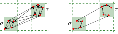
Figure 1: The vertices and edges of two neighboring cells of $G$ (left) and of $H$ (right)

The subgraph $H$ has vertex set $P$, and we pick its edges as follows (see also Figure 1): for each non-empty cell $\sigma\in\operatorname{\mathcal{Q}}_{0}$, we set $P_{\sigma}=P\cap\sigma$, and we compute the Euclidean minimum spanning tree (EMST) $T_{\sigma}$ of $P_{\sigma}$. For each edge $pq$ of $T_{\sigma}$, we add the directed edges $pq$ and $qp$ to $H$. Then, for every cell $\tau\in N(\sigma)$, we check if there are any edges from $\sigma$ to $\tau$ in $G$. If so, we add an arbitrary such edge to $H$. We denote by $F$ the set of edges $pq$ such that $p$ and $q$ are in different cells. The following lemma summarizes the properties of $H$.

Lemma 4.3.

The graph $H$ has the following properties.

1. for any two vertices $p$ and $q$, $p$ can reach $q$ in $G$ if and only if $p$ can reach $q$ in $H$;

2. $H$ has $O(n)$ edges;

3. $H$ can be constructed in $O(n\log n)$ time; and

4. the straight line embedding of $H$ in the plane has $O(n)$ edge crossings.

Proof.

(i): All edges of $H$ are also edges of $G$: inside a non-empty cell $\sigma$, $P_{\sigma}$ induces a clique in $G$, and the edges of $H$ between cells lie in $G$ by construction. It follows that if $p$ can reach $q$ in $H$ then $p$ can reach $q$ in $G$.

To show the converse let $pq$ be an edge in $G$. We show that there is a path from $p$ to $q$ in $H$. If $pq$ lies in a cell $\sigma$ of $\operatorname{\mathcal{Q}}_{0}$, we take the path from $p$ to $q$ along the EMST $T_{\sigma}$. If $pq$ goes from a cell $\sigma$ to another cell $\tau$, then there is an edge $uv$ from $\sigma$ to $\tau$ in $H$, and we take the path in $T_{\sigma}$ from $p$ to $u$, then the edge $uv$, and finally the path in $T_{\tau}$ from $v$ to $q$.

(ii): For a nonempty cell $\sigma$, we create $|P_{\sigma}|-1$ edges inside $\sigma$. Furthermore, since $|N(\sigma)|$ is constant, there are $O(1)$ edges between points in $\sigma$ and points in other cells. Thus, $H$ has $O(n)$ edges.

(iii): Since we assumed that we can find the cell for a vertex $p\in P$ in constant time, we can easily compute the sets $P_{\sigma}$, for every nonempty $\sigma\in\operatorname{\mathcal{Q}}_{0}$, in $O(n)$ time. Computing the EMST $T_{\sigma}$ for a cell $\sigma$ requires $O(|P_{\sigma}|\log|P_{\sigma}|)$ time, which sums to $O(n\log n)$ time for all cells. To find the edges of $F$ (i.e., edges between neighboring cells) we build a Voronoi diagram together with a point location structure for each set $P_{\sigma}$. This takes $O(n\log n)$ time for all cells. Let $\sigma$ and $\tau$ be two neighboring cells. For each point in $P_{\sigma}$, we locate the nearest neighbor in $P_{\tau}$ using the Voronoi diagram of $P_{\tau}$. If there is a point $p\in P_{\sigma}$ whose nearest neighbor $q\in P_{\tau}$ lies in $D(p)$, we add the edge $pq$ to $H$, and we proceed to the next pair of neighboring cells. Since $|N(\sigma)|$ is constant, a point participates in $O(1)$ point location queries, each taking $O(\log n)$ time. The total running time of all point location queries is $O(n\log n)$.

(iv): Clearly each such crossing involves at least one edge of $F$ (the set of edges between points in different cells). Each edge $e$ of $H$ intersects $O(1)$ cells $\sigma$ (this holds for edges in $F$ and trivially holds for edges inside cells). Each intersection of $e$ with an edge of $F$ must occur in one of these $O(1)$ cells that $e$ intersects. On the other hand, each cell $\sigma$ intersects only $O(1)$ edges of $F$. So there are only $O(1)$ intersections per edge of $H$. ∎

Making $G$ Planar.

We now describe how to turn a graph $G$, embedded in the plane, into a planar graph. (This transformation can be applied to any graph embedded in the plane. But Lemma 4.6 applies only if $G$ is a transmission graph.) Suppose an edge $pq$ and an edge $uv$ of $G$ cross at a point $x$. To eliminate this crossing, we add the intersection point $x$ as a new vertex to the graph, and we replace $pq$ and $uv$ by the four new edges $px$, $xq$, $ux$ and $xv$. Furthermore, if $qp$ is an edge of $G$, we replace it by the two edges $qx$, $xp$, and if $vu$ is an edge of $G$, we replace it by the two edges $vx$, $xu$. See Figure 2. We say that this resolves the crossing between $p,q,u$ and $v$. Let $\widetilde{G}$ be the graph obtained by iteratively resolving all crossings in $G$.

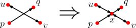
Figure 2: Resolving a crossing. Since the edge $vu$ exists, we also add $vx$ and $xu$ as edges.

First, we want to show that resolving crossings keeps the local reachability relation between the four vertices of the crossing edges. Intuitively speaking, the restriction $\Psi<3$ forces the vertices to be close together. This guarantees the existence of additional edges between $p,q,u,v$ in $G$, and these edges justify the new paths introduced by resolving the crossing.

To formally prove this, we first need a geometric observation. For a point $p\in P$, let $D(p,r)$ and $C(p,r)$ be the disk and the circle around $p$ with radius $r$.

Lemma 4.4.

Let $p,q$ be two points in $\mathbb{R}^{2}$ with $|pq|=\sqrt{3}$.

1. Let $a\in C(p,1)\cap C(q,1)$, and let $b\in C(p,r)\cap C(q,r)$ for some $r\in[1,\sqrt{3})$ such that $a$ and $b$ lie on different sides of the line through $p$ and $q$. Then $|ab|\geq r$. See Figure 3(a).

2. Let $\{a,b\}=C(p,\sqrt{3})\cap C(q,1)$. Then, $|ab|>\sqrt{3}$. See Figure 3(b).

Proof.

(i): Let $x$ be the intersection point of the line segments $\overline{pq}$ and $\overline{ab}$. Then $|ab|=|ax|+|xb|$. Using that $|pa|=1$ and $|px|=\sqrt{3}/2$, the Pythagorean Theorem gives $|xa|=1/2$. Similarly, we can compute $|xb|$ as a function of $r$: with $|pb|=r$ we get $|xb|=\sqrt{r^{2}-3/4}$. We want to show that

$$r\leq|ab|=1/2+\sqrt{r^{2}-3/4}\;\Leftrightarrow\; r^{2}\leq 1/4+\sqrt{r^{2}-3/4}+r^{2}-3/4\;\Leftrightarrow\;1\leq r^{2},$$

which holds since $r\in[1,\sqrt{3})$.

(ii): Let $x$ be the intersection point of $\overline{pq}$ and $\overline{ab}$. Use the Pythagorean Theorem in the triangles $\triangle apx$ and $\triangle aqx$ in Figure 3(b) we get that $|ab|=2\sqrt{11/12}>\sqrt{3}$. ∎

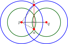
(a)

(b)

Figure 3: The cases (i) and (ii) of Lemma 4.4.

Lemma 4.5.

Suppose that $pq$ and $uv$ are edges in a transmission graph $G$ that cross. Let $G^{\prime}\subseteq G$ be the transmission graph induced by $p,q,u$ and $v$. If $\Psi<\sqrt{3}$, then $p$ reaches $v$ in $G^{\prime}$ and $u$ reaches $q$ in $G^{\prime}$.

Proof.

We may assume that $r_{p}\geq r_{u}$. Furthermore, we assume that $r_{q}=r_{v}=1$. This does not add new edges and thus reachability in the new graph implies reachability in $G^{\prime}$. We show that if either $u$ does not reach $q$ (case 1) or $p$ does not reach $v$ (case 2), then $|uv|>r_{u}$. Hence $uv$ cannot be an edge of $G^{\prime}$ despite our assumption.

Case 1: $u$ does not reach $q$. Then we have $p\notin D(u)$, $q\notin D(u)$, $p\notin D(v)$ and $q\notin D(v)$. Equivalently this gives $u\notin D(p,r_{u})\cup D(q,r_{u})$ and $v\notin D(p,1)\cup D(q,1)$. Thus, the positions of $u$ and $v$ that minimize $|uv|$ are the intersections $u\in C(p,r_{u})\cap C(q,r_{u})$ and $v\in C(p,1)\cap C(q,1)$ on different sides of the line through $p$ and $q$. To further minimize $|uv|$, observe that $|uv|$ depends on the distance of $p$ and $q$ and that $|uv|$ strictly decreases as $|pq|$ grows, i.e., as $|pq|$ approaches $\sqrt{3}$. For the limit case $|pq|=\sqrt{3}$, we are in the situation of Lemma 4.4(i) with $a=u$ and $b=v$ and thus we would get $|uv|\geq r_{u}$. But since $\Psi<\sqrt{3}$, we must have $|pq|<\sqrt{3}$ and by strict monotonicity, it follows that $|uv|>r_{u}$, as desired.

Case 2: $p$ does not reach $v$. Then we have $u\notin D(p)$, $v\notin D(p)$, $u\notin D(q)$ and $v\notin D(q)$. We scale everything, such that $r_{p}=\sqrt{3}$, and we reduce $r_{v}$, $r_{q}$ once again to $1$. Now, the positions of $u$ and $v$ minimizing $|uv|$ are $\{u,v\}=C(p,\sqrt{3})\cap C(q,1)$. As above, further minimizing $|uv|$ gives $|pq|=\sqrt{3}$. By Lemma 4.4(ii), we have $|uv|>\sqrt{3}$ and thus $uv$ cannot be an edge of $G^{\prime}$ (note that even after scaling we have $r_{u}\leq\sqrt{3}$ since we assumed that $r_{p}\geq r_{u}$). ∎

Recall that we iteratively resolve crossings in $G$ and call the resulting graph $\widetilde{G}$. Next, we show that for any $p,q\in P$, if $p$ can reach $q$ in $\widetilde{G}$, then $p$ can also reach $q$ in $G$. This seems to be a bit more difficult than what one might expect, because when resolving the crossings, we introduce new vertices and edges to which Lemma 4.5 is not directly applicable (since the intermediate graph is not a transmission graph). Thus, a priori, we cannot exclude the possiblity that there are new reachabilities in $\widetilde{G}$ that use the additional vertices and edges.

Lemma 4.6.

Let $G$ be a transmission graph of a set $P$ of points with $\Psi<\sqrt{3}$. Let $\widetilde{G}$ be the planar graph obtained from $G$ by resolving all crossings as described above. Then, for any two points $p,q\in P$, $p$ can reach $q$ in $\widetilde{G}$ if and only if $p$ can reach $q$ in $G$.

Proof.

If $p$ and can reach $q$ in $G$ then it immediately follows from our construction that $p$ can reach $q$ in $\widetilde{G}$. We now prove the converse.

Each edge $e$ of $\widetilde{G}$ lies on an edge $e^{\prime}$ of $G$ with the same direction as $e$. We call $e^{\prime}$ the supporting edge of $e$. Consider a path $\pi$ from $p$ to $q$ in $\widetilde{G}$. A supporting switch on $\pi$ is a pair of consecutive edges $\langle e,e^{\prime}\rangle$ on $\pi$ such that the supporting edge of $e$ and the supporting edge of $e^{\prime}$ are different.

A pair $p,q\in P$ such that $p$ can reach $q$ in $\widetilde{G}$, but not in $G$ is called a bad pair. The proof is by contradition. We assume that there exists a bad pair and among all bad pairs, we pick a pair $p,q$ and a path $\pi$ from $p$ to $q$ (in $\widetilde{G}$) such that $\pi$ consists of a minimum number of supporting switches, among all paths (in $\widetilde{G}$) between bad pairs. Let $\langle e_{1},e^{\prime}_{1}\rangle,\langle e_{2},e^{\prime}_{2}\rangle,\dots,\langle e_{k-1},e^{\prime}_{k-1}\rangle$ be the supporting switches along $\pi$ and let $p_{1}q_{1},\dots,p_{k}q_{k}$ be the sequence of supporting edges as they are visited along $\pi$ ($p_{1}=p$, $q_{k}=q$). That is $e_{1}$ is on $p_{1}q_{1}$, for $i=1,\ldots,k-2$, $e^{\prime}_{i}$ and $e_{i+1}$ are on $p_{i+1}q_{i+1}$, and $e^{\prime}_{k-1}$ is on $p_{k}q_{k}$. Let $x_{i}$ be the common vertex of $e_{i}$ and $e^{\prime}_{i}$. The vertex $x_{i}$ is on the segments $\overline{p_{i}q_{i}}$ and $\overline{p_{i+1}q_{i+1}}$.

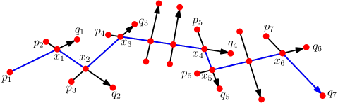
Figure 4: A path (blue) with $k=7$ supporting edges that is in $\widetilde{G}$ but not in $G$.

Claim 4.7.

The following holds in $G$: (P1) $p_{1}$ reaches $q_{2},\dots,q_{k-1}$; (P2) $p_{2},\dots,p_{k}$ reach $q_{k}$; (P3) $p_{1}$ and $q_{1}$ do not reach $p_{2},\dots,p_{k}$; and (P4) there is no edge $q_{i}p_{i}$, for $i\geq 2$. Furthermore, for $i=1,\dots,k-1$, we have that (P5) the vertex $x_{i}$ is in the interior of $\overline{p_{i}q_{i}}$ and $\overline{p_{i+1}q_{i+1}}$ and (P6) $x_{i+1}$ lies in the interior of $\overline{x_{i}q_{i+1}}$.

Proof.

P1 and P2 follow from the minimality of $\pi$, and P3 follows from P2. For P4, assume that $G$ contains an edge $q_{i}p_{i}$, for $i\geq 2$. By P1, $p_{1}$ reaches $q_{i}$ in $G$ and thus $p_{1}$ reaches $p_{i}$, despite P3. For P5, notice that if $x_{i}$ is not in the interior of $\overline{p_{i}q_{i}}$ and $\overline{p_{i+1}q_{i+1}}$, then $x_{i}=q_{i}=p_{i+1}$. But then, by P1, $p_{1}$ reaches $q_{i}=p_{i+1}$, despite P3. P6 is immediate from P5 and the fact that $p_{i+1}q_{i+1}$ cannot be equal to $q_{i}p_{i}$. ∎

By Lemma 4.5, we have $k\geq 3$, since for two crossing edges ($k=2$) no new reachabilities between the endpoints are created. We now argue that the path $\pi$ cannot exist. Since $p_{1}q_{1}$ and $p_{2}q_{2}$ cross, Lemma 4.5 implies that $G$ contains at least one of $p_{1}p_{2},q_{1}p_{2},p_{1}q_{2}$, or $q_{1}q_{2}$. This is because by Lemma 4.5, in the induced subgraph for $p_{1}$, $p_{2}$, $q_{1}$, $q_{2}$, the vertex $p_{1}$ can reach $q_{2}$, and this requires that at least one of the edges $p_{1}p_{2},q_{1}p_{2},p_{1}q_{2}$, or $q_{1}q_{2}$ be present. By P3, neither $p_{1}p_{2}$ nor $q_{1}p_{2}$ exist. There are two cases, depending on whether $G$ contains $p_{1}q_{2}$, or $q_{1}q_{2}$ (see Fig. 5). Each case leads to a contradiction with the minimality of $\pi$.

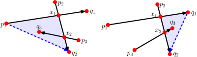
Figure 5: Either $p_{1}q_{2}$ or $q_{1}q_{2}$ locks $x_{3}$ in the corresponding triangle.

Case 1. $G$ contains $p_{1}q_{2}$. Consider the triangle $\triangle=\triangle p_{1}x_{1}q_{2}$. Since $q_{2},x_{1}\in D(p_{1})$, we have $\triangle\subset D(p_{1})$. Thus, by P3, none of $p_{2},\dots,p_{k}$ may lie inside $\triangle$. By P6, $p_{3}q_{3}$ intersects the boundary of $\triangle$ in the line segment $\overline{x_{1}q_{2}}$. First, suppose that $k=3$. In this case $q_{3}\not\in\triangle$ (otherwise $p_{1}$ could reach $q_{3}$). Thus, $p_{3}q_{3}$ intersects the boundary of $\triangle$ twice, so $p_{3}q_{3}$ either intersects $p_{1}q_{1}$ or $p_{1}q_{2}$. In both cases, Lemma 4.5 shows that $p_{1}$ reaches $q_{3}$. Thus, we must have $k\geq 4$.

We now prove that the intersection $x_{3}$ of $p_{3}q_{3}$ and $p_{4}q_{4}$ must lie in $\triangle$. If $p_{3}q_{3}$ intersects $\triangle$ once, then $q_{3}\in\triangle$, and therefore $x_{3}$, that by P6 must lie on the segment $x_{2}q_{3}$, is in $\triangle$. So assume that $p_{3}q_{3}$ intersects $\triangle$ twice, and let $y$ be the second intersection point of $p_{3}q_{3}$ with the boundary of $\triangle$. We claim that $y$ follows $x_{2}$ along $p_{3}q_{3}$. Assume otherwise, then since by P6, $x_{3}$ follows $x_{2}$ on $p_{3}q_{3}$, we can construct a path with fewer supporting switches than $\pi$: If $y\in\overline{p_{1}x_{1}}$, we omit $p_{2}q_{2}$ and if $y\in p_{1}q_{2}$, we omit $p_{2}q_{2}$ and substitute $p_{1}q_{1}$ by $p_{1}q_{2}$. By the same argument, $x_{3}$ cannot follow $y$ on $p_{3}q_{3}$. Thus, $x_{3}$ lies on the line segment $\overline{x_{2}y}\subset\triangle$. This concludes the proof that $x_{3}\in\triangle$. Now, consider the segment $\overline{p_{4}x_{3}}$. Since we observed that $p_{4}\not\in\triangle$, we have that $\overline{p_{4}x_{3}}$ intersects $\triangle$, and we can again replace $\pi$ by a path with fewer supporting switches from $p$ to $q$.

Case 2. $G$ contains $q_{1}q_{2}$. Consider the triangle $\triangle=\triangle x_{1}q_{1}q_{2}$. We claim that $\triangle\subset D(p_{1})\cup D(q_{1})$. Then the argument continues analogously to Case 1. In particular, P3 still shows that none of $p_{2},\dots,p_{k}$ may lie inside $\triangle$. The case $k=3$ can again be ruled out, because then $p_{3}q_{3}$ would have to intersect either $p_{1}q_{1}$ or $q_{1}q_{2}$, and Lemma 4.5 would show that $p_{1}$ can reach $q_{3}$. For $k\geq 4$, we can again show that $x_{3}$ would have to lie inside $\triangle$ (otherwise, we could obtain bad pair with fewer supporting switches by either omitting $p_{2}q_{2}$ or omitting $p_{2}q_{2}$ and substituting $p_{1}q_{1}$ by $q_{1}q_{2}$). Thus, by considering the segment $\overline{p_{4}x_{3}}$, we could again find a bad pair with fewer supporting switches.

We now show that that $\triangle\subset D(p_{1})\cup D(q_{1})$. If $x_{1}\in D(q_{1})$ then $\triangle\subseteq D(q_{1})$ and we are done. Otherwise, let $D(x_{1})\subseteq D(p_{1})$ be the disk with center $x_{1}$ and $q_{1}$ on its boundary. We claim that $D(x_{1})$ contains $\triangle\setminus D(q_{1})$. Let $y$ be the intersection of $C(q_{1})$ with $x_{1}q_{2}$. Since $|q_{1}y|\geq|q_{1}q_{2}|$, $\angle q_{1}yq_{2}\leq\pi/2$. Therefore $\angle q_{1}yx_{1}\geq\pi/2$ and $|x_{1}y|<|x_{1}q_{1}|$. This implies that $x_{1}y$ is contained in $D(x_{1})$ and therefore $\triangle\setminus D(q_{1})$ is contained in $D(x_{1})$ as required. ∎

Putting it together.

Let $G$ be a transmission graph of a set $P$ of points, given by the point set $P$ and the associated radii. To prove Lemma 4.1, we first construct the sparse subgraph $H$ of $G$ as in Lemma 4.3 in time $O(n\log n)$. Then we iteratively resolve the crossings in $H$ to obtain $\widetilde{H}$. Since $H$ has $O(n)$ crossings that can be found in $O(n)$ time, this takes $O(n)$ time.

The graph $H$ is not necessarily a transmission graph. Therefore, we cannot directly apply Lemma 4.6 to $H$ and conclude that $\widetilde{H}$ preserves the reachability relation (between points of $P$) of $H$ and therefore of $G$. Nevertheless, in the following lemma, we will prove that $\widetilde{H}$ and $G$ do have the same reachability relation between points of $P$.

Lemma 4.8.

Let $G$ be a transmission graph on a set $P$ of points. Let $H$ be a sparse subgraph of $G$ constructed as in Lemma 4.3 and let $\widetilde{H}$ be the planar graph obtained by resolving the crossings in $H$ as described above. Then for any two points $p,q\in P$, $p$ can reach $q$ in $\widetilde{H}$ if and only if $p$ can reach $q$ in $G$.

Proof.

Let $\widetilde{G}$ be the graph obtained by resolving the crossings in $G$, as described above. If $p$ can reach $q$ in $G$, then by Lemma 4.3, $p$ can reach $q$ in $H$, and by the definition of the way we resolve crossings, $p$ can reach $q$ also in $\widetilde{H}$.

Conversely, if $p$ can reach $q$ in $\widetilde{H}$, then $p$ can reach $q$ in $\widetilde{G}$, because a subdivision of every edge of $\widetilde{H}$ is contained in $\widetilde{G}$. Therefore, by Lemma 4.6, $p$ can reach $q$ in $G$. ∎

4.2 Polynomial Dependence on $\Psi$

We now present a standard reachability oracle whose performance parameters depend polynomially on the radius ratio $\Psi$. Together with Theorem 2.1 we will obtain the following result:

Theorem 4.9.

Let $G$ be the transmission graph for a set $P\subset\mathbb{R}^{2}$ of $n$ points. We can construct a geometric reachability oracle for $G$ with $S(n)=O(\Psi^{3}n^{3/2})$ and $Q(n)=O(\Psi^{3}\sqrt{n})$ in time $O(\Psi^{3}n^{3/2})$.

Our approach is based on a geometric separator theorem for planar disks. Let $\operatorname{\mathcal{D}}$ be the set of disks associated with the points in $P$. For a subset ${\mathcal{E}}$ of $\operatorname{\mathcal{D}}$ we write $\bigcup{\mathcal{E}}:=\bigcup_{D\in{\mathcal{E}}}D$ and we let $\mu({\mathcal{E}})$ be the area occupied by $\bigcup{\mathcal{E}}$. Alber and Fiala show how to find a separator for $\operatorname{\mathcal{D}}$ with respect to $\mu(\cdot)$ [1].

Theorem 4.10 (Theorem 4.12 in [1]).

There exist positive constants $\alpha<1$ and $\beta$ such that the following holds: let $\operatorname{\mathcal{D}}$ be a set of $n$ disks and let $\Psi$ be the ratio of the largest and the smallest radius in $\operatorname{\mathcal{D}}$. Then we can find in $O(\Psi^{2}n)$ time a partition ${\mathcal{A}}\cup{\mathcal{B}}\cup{\mathcal{S}}$ of $\operatorname{\mathcal{D}}$ satisfying (i) $\bigcup{\mathcal{A}}\cap\bigcup{\mathcal{B}}=\emptyset$, (ii) $\mu({\mathcal{S}})\leq\beta\Psi^{2}\sqrt{\mu(\operatorname{\mathcal{D}})}$ and (iii) $\mu({\mathcal{A}}),\mu({\mathcal{B}})\leq\alpha\mu(\operatorname{\mathcal{D}})$.

Since any directed path in $G$ lies completely in $\bigcup{\mathcal{D}}$, any path from a vertex of a disk in ${\mathcal{A}}$ to a vertex of a disk in ${\mathcal{B}}$ needs to use at least one vertex of a disk in ${\mathcal{S}}$, see Figure 6. (Notice that there may not be a path from a center $p$ of a disk in ${\mathcal{A}}$ to another center $q$ of a disk in ${\mathcal{A}}$ containing only centers of disks in ${\mathcal{A}}$. It may be that every path from $p$ to $q$ goes through a center corresponding to a disk in ${\mathcal{S}}$.) Since $\mu({\mathcal{S}})$ is small, we can approximate $\bigcup{\mathcal{S}}$ with a few grid cells. We choose the diameter of the cells small enough such that all vertices in one cell form a clique and are equivalent in terms of reachability. We can thus pick one vertex per cell and store the reachability information for it. Applying this idea recursively gives a separator tree that allows us to answer reachability queries efficiently. The details follow.

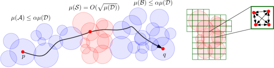
Figure 6: Any path from ${\mathcal{A}}$ to ${\mathcal{B}}$ needs to use at least one vertex of ${\mathcal{S}}$. Since $\mu({\mathcal{S}})$ is small, we can approximate $\bigcup{\mathcal{S}}$ with few grid cells.

Preprocessing Algorithm and Space Requirement.

For the preprocessing phase, consider the grid $\operatorname{\mathcal{Q}}=\operatorname{\mathcal{Q}}_{0}$ whose cells have diameter $1$. All vertices in a single cell form a clique in $G$, so the reachability information of all vertices in a grid cell is the same and it suffices to compute this information only for one such vertex. For each non-empty cell $\sigma\in\operatorname{\mathcal{Q}}$, we pick an arbitrary vertex $p_{\sigma}\in P\cap\sigma$ as the representative of $\sigma$. For a subset ${\mathcal{C}}\subset{\mathcal{D}}$ of disks we denote the set of representatives of the non-empty cells containing centers of the disks in ${\mathcal{C}}$ by $R_{\mathcal{C}}$.

We recursively create a separator tree $T$ that contains all the required reachability information. Each node $v$ of $T$ corresponds to an induced subgraph of the transmission graph and the root corresponds to the entire transmission graph. We construct the tree top down. Let $G_{v}$ be the subgraph associated with a node $v$ and let ${\mathcal{D}}_{v}$ be the set of disks of the vertices of $G_{v}$. We compute a separator ${\mathcal{S}}_{v}$ and subsets ${\mathcal{A}}_{v},{\mathcal{B}}_{v}$, satisfying the conditions of Theorem 4.10 for $G_{v}$. Let $Q_{v}$ be all cells in $\operatorname{\mathcal{Q}}$ containing centers of disks of ${\mathcal{S}}_{v}$. Let $R_{v}$ be the set of representatives of $Q_{v}$, and let ${\mathcal{C}}_{v}\subset{\mathcal{D}}_{v}$ be all disks with centers in $Q_{v}$ (Note that ${\mathcal{C}}_{v}$ contains ${\mathcal{S}}_{v}$). For each $r\in R_{v}$, we store all the disk centers of ${\mathcal{D}}_{v}$ that $r$ can reach and all the disk centers of ${\mathcal{D}}_{v}$ that can reach $r$ in $G_{v}$. We recursively compute separator trees for the transmission graphs induce by the centers of ${\mathcal{A}}_{v}\setminus{\mathcal{C}}_{v}$ and the centers of ${\mathcal{B}}_{v}\setminus{\mathcal{C}}_{v}$. The roots of these trees are children of $v$ in $T$.

To obtain the required reachability information at a node $v$ of $T$, we compute a $2$-spanner $H_{v}$ for the transmission graph $G_{v}$, as in Theorem 2.2. Since we are only interested in the reachability properties of the spanner, $\varepsilon=1$ (or any constant) suffices. For each $r\in R_{v}$, we compute a BFS tree in $H_{v}$ with root $r$. Next, we reverse all edges in $H_{v}$, and we again compute BFS-trees for all $r\in R_{v}$ in the transposed graph. This gives the required reachability information for $v$.

As $T$ has $O(\log n)$ levels, the total running time for computing the spanners is $O(n\log n(\log n+\log\Psi))$. Since the spanners are sparse, the time for computing a single BFS-tree associated with a node $v$ is $O(|{\mathcal{D}}_{v}|)$. It follows that the time for computing all BFS-trees at $v$ is $O(|{\mathcal{D}}_{v}|\cdot|R_{v}|)$ and the time to compute all BFS trees of all nodes of the separator tree $T$ is $O(\sum_{v\in T}|{\mathcal{D}}_{v}|\cdot|R_{v}|)$. To bound this sum, we need the following lemma.

Lemma 4.11.

Let ${\mathcal{E}}$ be a set of $n$ disks with radius at least $1$. Then the number of cells in $\operatorname{\mathcal{Q}}_{0}$ that intersect $\bigcup{\mathcal{E}}$ is $O(\mu({\mathcal{E}}))$.

Proof.

Let $S\subset\operatorname{\mathcal{Q}}_{0}$ be the set of all cells that intersect $\bigcup{\mathcal{E}}$. For $\sigma\in S$, the neighborhood of $\sigma$ is defined as the region consisting of $\sigma$ and its eight surrounding cells. Let $S^{\prime}\subseteq S$ be a maximal subset of cells in $S$ whose neighborhoods are pairwise disjoint. Then, $|S|=O(|S^{\prime}|)$. Now, let $\sigma\in S^{\prime}$. Since all disks in ${\mathcal{E}}$ have radius at least $1$, there is a disk $D^{\prime}$ (not necessarily in ${\mathcal{E}}$) of radius exactly $1/(2\sqrt{2})$ such that $D^{\prime}\subseteq\bigcup{\mathcal{E}}$ and such that $D^{\prime}$ intersects the boundary of $\sigma$. Thus, the intersection of $\bigcup{\mathcal{E}}$ and the neighborhood of $\sigma$ contributes at least $\mu(D^{\prime})=\Omega(1)$ to $\mu({\mathcal{E}})$. Since the neighborhoods for the cells in $S^{\prime}$ are pairwise disjoint, it follows that $|S|=O(|S^{\prime}|)=O(\mu({\mathcal{E}}))$, as claimed. ∎

Now, by Lemma 4.11, we have $|R_{v}|=O(\mu({\mathcal{S}}_{v}))$. Thus, if we denote by $L_{i}$ the nodes of the separator tree at level $i$ of the recursion, we get that the sum $\sum_{v}|{\mathcal{D}}_{v}|\cdot|R_{v}|$ is proportional to

$$\sum_{i\geq 0}\sum_{v\in L_{i}}|{\mathcal{D}}_{v}|\cdot\mu({\mathcal{S}}_{v}) \leq\sum_{i\geq 0}\sum_{v\in L_{i}}|{\mathcal{D}}_{v}|\cdot\beta\Psi^{2}\sqrt{\mu({\mathcal{D}}_{v})}$$ (by Theorem 4.10(ii))

$$=\sum_{i\geq 0}\sum_{v\in L_{i}}|{\mathcal{D}}_{v}|\cdot\beta\Psi^{2}\sqrt{\alpha^{i}\mu({\mathcal{D}})}$$ (by Theorem 4.10(iii))

$$=\beta\Psi^{2}\sqrt{\mu({\mathcal{D}})}\sum_{i\geq 0}\alpha^{i/2}\sum_{v\in L_{i}}|{\mathcal{D}}_{v}|$$

$$\leq\beta\Psi^{2}n\sqrt{\mu({\mathcal{D}})}\sum_{i\geq 0}\alpha^{i/2} {\mathcal{D}}_{v}$$ (the at a level are disjoint)

$$=O(\Psi^{3}n^{3/2}) (\mu({\mathcal{D}})=O(\Psi^{2}n),\alpha<1)$$

Thus, the total preprocessing time is $O(n\log^{2}n+n\log\Psi+\Psi^{3}n^{3/2})=O(\Psi^{3}n^{3/2})$. The space requirement is also bounded by the preprocessing time.

Query Algorithm.

Let $p,q\in P$ be given. We assume that $p$ and $q$ are the representatives of their cells. (Otherwise we replace either $p$ or $q$ by its representative.) Let $v$ and $w$ be the nodes in $T$ with $p\in R_{v}$ and $q\in R_{w}$. Let $u$ be least common ancestor of $v$ and $w$. We can find $u$ by walking up the tree starting from $v$ and $w$ in $O(\log n)$ time. Let $L$ be the path from $u$ to the root of $T$. We check for each $r\in\bigcup_{x\in L}R_{x}$ whether $p$ can reach $r$ and whether $r$ can reach $q$. If so, we return YES. If there is no such vertex $r$ then we return NO. Since $|R_{x}|$ increases geometrically along $L$, the running time is dominated by the time for processing the root, which is $O(\Psi^{2}\mu({\mathcal{D}})^{1/2})$. Bounding $\mu({\mathcal{D}})$ by $O(\Psi^{2}n)$, we get that the total query time is $O(\Psi^{3}\sqrt{n})$.

It remains to argue that our query algorithm is correct. By construction, it follows that we return YES only if there is a path from $p$ to $q$. Now, suppose there is a path $\pi$ in $G$ from $p$ to $q$, where $p$ and $q$ are representatives of their grid cells with $p\neq q$. Let $v,w$ be the nodes in $T$ with $p\in R_{v}$ and $q\in R_{w}$. Let $u$ be their least common ancestor, and $L$ be the path from $u$ to the root. By construction, $\bigcup_{x\in L}{\mathcal{S}}_{x}$ contains a disk $D(r)$ of a vertex $r$ in $\pi$. Let $x$ be the node of $L$ closest to the root such that ${\mathcal{S}}_{x}$ contains such a disk, and let $r$ be a vertex on $\pi$ with $D(r)\in{\mathcal{S}}_{x}$. Let $r^{\prime}$ be the representative of the cell $\sigma$ containing $r$. Since the vertices in $\sigma$ constitute a clique, $p$ can reach $r^{\prime}$ and $r^{\prime}$ can reach $q$ in $G_{x}$. Thus, when walking along $L$, the algorithm will discover $r^{\prime}$ and the path from $p$ to $q$. Theorem 4.9 now follows.

4.3 Logarithmic Dependence on $\Psi$

Finally, we improve the dependence on $\Psi$ to be logarithmic, at the cost of a slight increase at the exponent of $n$. We prove the following theorem by constructing a standard reachability oracle and then using Theorem 2.1.

Theorem 4.12.

Let $G$ be the transmission graph for a set $P$ of $n$ points in the plane. We can construct a geometric reachability oracle for $G$ with $S(n)=O(n^{5/3}\log^{1/3}\Psi\log^{2/3}n)$ and $Q(n)=O(n^{2/3}\log^{1/3}\Psi\log^{2/3}n)$ that answers all queries correctly with high probability. The preprocessing time is $O(n^{5/3}(\log\Psi+\log n)\log^{1/3}\Psi\log^{2/3}n)$.

We scale everything such that the smallest radius in $P$ is $1$. Our approach is as follows: let $p,q\in P$. If there is a $p$-$q$-path with “many” vertices, we detect this by taking a large enough random sample $S\subseteq P$ and by storing the reachability information for every vertex in $S$. If there is a path from $p$ to $q$ with “few” vertices, then $p$ must be “close” to $q$, where “closeness” is defined relative to the largest radius along the path. The radii of the point of $P$ can lie in $O(\log\Psi)$ different scales, and for each scale we store local information to find such a “short” path.

Long Paths.

Let $0<\alpha<1$ be a parameter to be determined later. First, we show that a random sample can be used to detect paths with many vertices.

Lemma 4.13.

We can sample a set $S\subset P$ of size $O(n^{\alpha}\log n)$ such that the following holds with probability at least $1-1/n^{2}$: For any two points $p,q\in P$, if there is a path $\pi$ from $p$ to $q$ in $G$ with at least $n^{1-\alpha}$ vertices, then $\pi\cap S\neq\emptyset$.

Proof.

We take $S$ to be a random subset of size $m=4n^{\alpha}\ln n$ vertices from $P$. Now fix $p$ and $q$ and let $\pi$ be a path from $p$ to $q$ with $k\geq n^{1-\alpha}$ vertices. The probability that $S$ contains no vertex from $\pi$ is

$$\frac{\binom{n-k}{m}}{\binom{n}{m}} =\frac{(n-m)(n-m-1)\cdots(n-m-k+1)}{n(n-1)\cdots(n-k+1)}$$

$$=\left(1-\frac{m}{n}\right)\left(1-\frac{m}{n-1}\right)\cdots\left(1-\frac{m}{n-k-1}\right)\leq(1-m/n)^{k}\leq e^{-mk/n}\leq 1/n^{4},$$

by our choice of $m$. Since there are $n(n-1)$ ordered vertex pairs, the union bound shows that the probability that $S$ fails to detect a pair of vertices connected by a long path is at most $n(n-1)/n^{4}\leq 1/n^{2}$. ∎

We draw a sample $S$ as in Lemma 4.13, and for each $s\in S$, we store two Boolean arrays that indicate for each $p\in P$ whether $p$ can reach $s$ and whether $s$ can reach $p$. This requires $O(n^{1+\alpha}\log n)$ space. It remains to deal with vertices that are connected by a path with fewer than $n^{1-\alpha}$ vertices.

Short Paths.

Let $L=\lceil\log\Psi\rceil$. We consider the $L$ grids $\operatorname{\mathcal{Q}}_{0},\dots,\operatorname{\mathcal{Q}}_{L}$ (recall that the cells in $\operatorname{\mathcal{Q}}_{i}$ have diameter $2^{i}$). For each cell $\sigma\in\operatorname{\mathcal{Q}}_{i}$, let $R_{\sigma}\subseteq P$ be the vertices $p\in P\cap\sigma$ with $r_{p}\in[2^{i},2^{i+1})$. The set $R_{\sigma}$ forms a clique in $G$, and for each $p\in R_{\sigma}$, the disk $D(p)$ contains the cell $\sigma$. For every $i=0,\dots,L$ and for every $\sigma\in\operatorname{\mathcal{Q}}_{i}$ with $R_{\sigma}\neq\emptyset$, we fix an arbitrary representative point $r_{\sigma}\in R_{\sigma}$.

The neighborhood $N(\sigma)$ of $\sigma\in\operatorname{\mathcal{Q}}_{i}$ is defined as the set of all cells in $\operatorname{\mathcal{Q}}_{i}$ that have distance at most $2^{i+1}n^{1-\alpha}$ from $\sigma$. We have $|N(\sigma)|=O(n^{2-2\alpha})$. Let $P_{\sigma}\subseteq P$ be the vertices that lie in the cells of $N(\sigma)$.

For every vertex $p\in P$, and for every $i\in\{0,\dots,L\}$ we store two sorted lists of representative of cells $\sigma\in\operatorname{\mathcal{Q}}_{i}$ such that $p\in P_{\sigma}$. The first list contains all representatives $r_{\sigma}$, such that $p\in P_{\sigma}$ and $p$ can reach $r_{\sigma}$. The second list contains all representatives $r_{\sigma}$, such that $p\in P_{\sigma}$ and $r_{\sigma}$ can reach $p$. A vertex $p$ belongs to $O(n^{2-2\alpha}\log\Psi)$ sets $P_{\sigma}$, so the total space is $O(n^{3-2\alpha}\log\Psi)$.

Performing a Query.

Let $p,q\in P$ be given. To decide whether $p$ can reach $q$, we first check the Boolean tables for all $O(n^{\alpha}\log n)$ points in $S$. If there is an $s\in S$ such that $p$ reaches $s$ and $s$ reaches $q$, we return YES. If not, for $i\in\{0,\dots,L\}$, we consider the list of representatives that are reachable from $p$ in their neighborhood at level $i$ and the list of representatives that can reach $q$ in their neighborhood at level $i$. We check whether these lists contain a common element. Since the lists are sorted, this can be done in time linear in their size. If we find a common representative for some $i$, we return YES. Otherwise, we return NO.

We now prove the correctness of the query algorithm. First note that we return YES, only if there is a path from $p$ to $q$. Now suppose that there is a path $\pi$ from $p$ to $q$. If $\pi$ has at least $n^{1-\alpha}$ vertices, then by Lemma 4.13, the sample $S$ hits $\pi$ with probability at least $1-1/n^{2}$, and the algorithm returns YES. If $\pi$ has less than $n^{1-\alpha}$ vertices, let $r$ be the vertex of $\pi$ with the largest radius, and let $i$ be such that the radius of $r$ lies in $[2^{i},2^{i+1})$. Let $\sigma$ be the cell of $\operatorname{\mathcal{Q}}_{i}$ that contains $r$. Since $\pi$ has at most $n^{1-\alpha}$ vertices, and since each edge of $\pi$ has length at most $2^{i+1}$, the path $\pi$ lies entirely in $P_{\sigma}$ and in particular both $p$ and $q$ are in $P_{\sigma}$. Since $r\in R_{\sigma}$ and since $R_{\sigma}$ forms a clique in $G$, the representative point $r_{\sigma}$ of $\sigma$ can be reached from $p$ and can reach $q$. It follows from the definition of the sorted lists of representatives stored with $p$ and $q$, that $r_{\sigma}$ is contained in the list of representatives reachable from $p$ and in the list of representatives that can reach $q$. Our query algorithm detects this when it checks whether the corresponding lists for $p$ and $q$ at level $i$, have a nonempty intersection.

Time and Space Requirements.

We consider first the query time. To test if there is a long path from $p$ to $q$ we traverse $S$, and for every $s\in S$ we test, in $O(1)$ time, whether $p$ can reach $s$ and whether $s$ can reach $q$. This takes $O(|S|)=O(n^{\alpha}\log n)$ time. To test if there is a short path from $p$ to $q$ we use the lists of reachable representatives associated with $p$ and $q$ at each of the $O(\log\Psi)$ grids. At each level we step through two lists of size $O(n^{2-2\alpha})$. So in total we spend $O(n^{2-2\alpha}\log\Psi)$ time. We choose $\alpha$ to balance the times we spend to detect short and long paths. That is $\alpha$ satisfies

$$n^{\alpha}\log n=n^{2-2\alpha}\log\Psi\Leftrightarrow n^{\alpha}=n^{2/3}(\log\Psi/\log n)^{1/3}.$$

This yields $Q(n)=O(n^{2/3}\log^{1/3}\Psi\log^{2/3}n)$. This choice of $\alpha$ results in a space bound of $O(n^{5/3}\log^{1/3}\Psi\log^{2/3}n)$.

For the preprocessing algorithm, we first compute the reachability arrays for each $s\in S$. To do so, we build a 2-spanner $H$ for $G$ as in Theorem 2.2 in $O(n(\log n+\log\Psi))$ time. Then, for each $s\in S$ we perform a BFS search in $H$ and its transposed graph. This gives all vertices that $s$ can reach and all vertices that can reach $s$ in $O(n^{5/3}\log^{1/3}\Psi\log^{2/3}n)$ total time. For the short paths, the preprocessing algorithm goes as follows: For each $i=0,\dots,L$ and for each cell $\sigma\in\operatorname{\mathcal{Q}}_{i}$ that has a representative $r_{\sigma}$, we compute a 2-spanner $H_{\sigma}$ as in Theorem 2.2 for $P_{\sigma}$. For each representative $r_{\sigma}$, we do a BFS search in $H_{\sigma}$ and the transposed graph, each starting from $r_{\sigma}$. This gives all $p\in P_{\sigma}$ that can reach $r_{\sigma}$ and that are reachable from $r_{\sigma}$ via a short path. The running time is dominated by the time for constructing the spanners. Since each point $p\in P$ is contained in $O(n^{2-2\alpha}\log\Psi)=O(n^{2/3}\log^{1/3}\Psi\log^{2/3}n)$ different $P_{\sigma}$, and since constructing $H_{\sigma}$ takes $O(|P_{\sigma}|(\log\Psi+\log|P_{\sigma}|))$ time, the bound on the preprocessing time stated in Theorem 4.12 follows.

5 Conclusion

Transmission graphs constitute a natural class of directed graphs for which non-trivial reachability oracles can be constructed. As mentioned in the introduction, it seems to be a very challenging open problem to obtain similar results for general directed graphs. We believe that our results only scratch the surface of the possibilities offered by transmission graphs, and several interesting open problems remain.

All our results on 2-dimensional transmission graphs depend on the radius ratio $\Psi$. Whether this dependency can be avoided is a major open question. Our most efficient reachability oracle is for $\Psi<\sqrt{3}$. In this case the reachability relation in a transmission graph with $n$ vertices can be represented by the reachability relation in a planar graph with $O(n)$ vertices. However, it is not clear to us that the upper bound of $\sqrt{3}$ in this result is tight. Can we obtain a similar construction for, say, $\Psi=100$? Is there a way to represent the reachability relation in any transmission graph, regardless of $\Psi$, by the reachability relation in a planar graph with $o(n^{2})$ vertices? This would immediately imply a non-trivial reachability oracle for any value of $\Psi$.

Conversely, it is interesting to see if we can represent the reachability relation of an arbitrary directed graph using a transmission graph. If this is possible, the relevant questions are how many vertices such a transmission graph must have, what is the required radius ratio, and how fast can we compute it. A representation with not too many vertices and low radius ratio would lead to efficient reachability oracles for general directed graphs.

Acknowledgments.

We like to thank Günter Rote and the anonymous reviewers for valuable comments, in particular for pointing out a drastic simplification for the one-dimensional reachability oracle.

References

- [1] J. Alber and J. Fiala. Geometric separation and exact solutions for the parameterized independent set problem on disk graphs. J. Algorithms, 52(2):134–151, 2004.
- [2] S. Arikati, D. Z. Chen, L. P. Chew, G. Das, M. Smid, and C. D. Zaroliagis. Planar spanners and approximate shortest path queries among obstacles in the plane. In Proc. 4th Annu. European Sympos. Algorithms (ESA), pages 514–528, 1996.
- [3] M. de Berg, O. Cheong, M. van Kreveld, and M. H. Overmars. Computational Geometry: Algorithms and Applications. Springer-Verlag, 3rd edition, 2008.
- [4] D. Z. Chen and J. Xu. Shortest path queries in planar graphs. In Proc. 32nd Annu. ACM Sympos. Theory Comput. (STOC), pages 469–478, 2000.
- [5] E. Cohen, E. Halperin, H. Kaplan, and U. Zwick. Reachability and distance queries via 2-hop labels. SIAM J. Comput., 32(5):1338–1355, 2003.
- [6] H. N. Djidjev. Efficient algorithms for shortest path queries in planar digraphs. In Proc. 22nd International Workshop on Graph-Theoretic Concepts in Computer Science (WG), pages 151–165, 1996.
- [7] G. N. Federickson. Fast algorithms for shortest paths in planar graphs, with applications. SIAM J. Comput., 16(6):1004–1022, 1987.
- [8] J. Holm, E. Rotenberg, and M. Thorup. Planar reachability in linear space and constant time. In Proc. 56th Annu. IEEE Sympos. Found. Comput. Sci. (FOCS), pages 370–389, 2015.
- [9] H. Kaplan, W. Mulzer, L. Roditty, and P. Seiferth. Spanners and reachability oracles for directed transmission graphs. In Proc. 31st Int. Sympos. Comput. Geom. (SoCG), pages 156–170, 2015.
- [10] H. Kaplan, W. Mulzer, L. Roditty, and P. Seiferth. Spanners for directed transmission graphs. SIAM J. Comput., 47(4):1585–1609, 2018.
- [11] D. Peleg and L. Roditty. Localized spanner construction for ad hoc networks with variable transmission range. ACM Transactions on Sensor Networks (TOSN), 7(3):25:1–25:14, 2010.
- [12] M. Pǎtraşcu. Unifying the landscape of cell-probe lower bounds. SIAM J. Comput., 40(3):827–847, 2011.
- [13] M. Thorup. Compact oracles for reachability and approximate distances in planar digraphs. J. ACM, 51(6):993–1024, 2004.
- [14] P. von Rickenbach, R. Wattenhofer, and A. Zollinger. Algorithmic models of interference in wireless ad hoc and sensor networks. IEEE/ACM Transactions on Networking, 17(1):172–185, 2009.