Sparse Exchangeable Graphs and Their Limits
via Graphon Processes

Abstract

In a recent paper, Caron and Fox suggest a probabilistic model for sparse graphs which are exchangeable when associating each vertex with a time parameter in $\mathbb{R}_{+}$. Here we show that by generalizing the classical definition of graphons as functions over probability spaces to functions over $\sigma$-finite measure spaces, we can model a large family of exchangeable graphs, including the Caron-Fox graphs and the traditional exchangeable dense graphs as special cases. Explicitly, modelling the underlying space of features by a $\sigma$-finite measure space $(S,\mathcal{S},\mu)$ and the connection probabilities by an integrable function $W\colon S\times S\to[0,1]$, we construct a random family $(G_{t})_{t\geq 0}$ of growing graphs such that the vertices of $G_{t}$ are given by a Poisson point process on $S$ with intensity $t\mu$, with two points $x,y$ of the point process connected with probability $W(x,y)$. We call such a random family a graphon process. We prove that a graphon process has convergent subgraph frequencies (with possibly infinite limits) and that, in the natural extension of the cut metric to our setting, the sequence converges to the generating graphon. We also show that the underlying graphon is identifiable only as an equivalence class over graphons with cut distance zero. More generally, we study metric convergence for arbitrary (not necessarily random) sequences of graphs, and show that a sequence of graphs has a convergent subsequence if and only if it has a subsequence satisfying a property we call uniform regularity of tails. Finally, we prove that every graphon is equivalent to a graphon on $\mathbb{R}_{+}$ equipped with Lebesgue measure.

Keywords: graphons, graph convergence, sparse graph convergence, modelling of sparse networks, exchangeable graph models

1 Introduction

The theory of graphons has provided a powerful tool for sampling and studying convergence properties of sequences of dense graphs. Graphons characterize limiting properties of dense graph sequences, such as properties arising in combinatorial optimization and statistical physics. Furthermore, sequences of dense graphs sampled from a (possibly random) graphon are characterized by a natural notion of exchangeability via the Aldous-Hoover theorem. This paper presents an analogous theory for sparse graphs.

In the past few years, graphons have been used as non-parametric extensions of stochastic block models, to model and learn large networks. There have been several rigorous papers on the subject of consistent estimation using graphons (see, for example, papers by Bickel and Chen, 2009, Bickel, Chen, and Levina, 2011, Rohe, Chatterjee, and Yu, 2011, Choi, Wolfe, and Airoldi, 2012, Wolfe and Olhede, 2013, Gao, Lu, and Zhou, 2015, Chatterjee, 2015, Klopp, Tsybakov, and Verzelen, 2017, and Borgs, Chayes, Cohn, and Ganguly, 2015, as well as references therein), and graphons have also been used to estimate real-world networks, such as Facebook and LinkedIn (E. M. Airoldi, private communication, 2015). This makes it especially useful to have graphon models for sparse networks with unbounded degrees, which are the appropriate description of many large real-world networks.

In the classical theory of graphons as studied by, for example, Borgs, Chayes, Lovász, Sós, and Vesztergombi (2006), Lovász and Szegedy (2006), Borgs, Chayes, Lovász, Sós, and Vesztergombi (2008), Bollobás and Riordan (2009), Borgs, Chayes, and Lovász (2010), and Janson (2013), a graphon is a symmetric $[0,1]$-valued function defined on a probability space. In our generalized theory we let the underlying measure space of the graphon be a $\sigma$-finite measure space; i.e., we allow the space to have infinite total measure. More precisely, given a $\sigma$-finite measure space $\mathscr{S}=(S,\mathcal{S},\mu)$ we define a graphon to be a pair $\mathcal{W}=(W,\mathscr{S})$, where $W\colon S\times S\to\mathbb{R}$ is a symmetric integrable function, with the special case when $W$ is $[0,1]$-valued being most relevant for the random graphs studied in the current paper. We present a random graph model associated with these generalized graphons which has a number of properties making it appropriate for modelling sparse networks, and we present a new theory for convergence of graphs in which our generalized graphons arise naturally as limits of sparse graphs.

Given a $[0,1]$-valued graphon $\mathcal{W}=(W,\mathscr{S})$ with $\mathscr{S}=(S,\mathcal{S},\mu)$ a $\sigma$-finite measure space, we will now define a random process which generalizes the classical notion of $\mathcal{W}$-random graphs, introduced in the statistics literature (Hoff, Raftery, and Handcock, 2002) under the name latent position graphs, in the context of graph limits (Lovász and Szegedy, 2006) as $\mathcal{W}$-random graphs, and in the context of extensions of the classical random graph theory (Bollobás, Janson, and Riordan, 2007) as inhomogeneous random graphs. Recall that in the classical setting where $\mathcal{W}$ is defined on a probability space, $\mathcal{W}$-random graphs are generated by first choosing $n$ points $x_{1},\dots,x_{n}$ i.i.d. from the probability distribution $\mu$ over the feature space $S$, and then connecting the vertices $i$ and $j$ with probability $W(x_{i},x_{j})$. Here, inspired by Caron and Fox (2014), we generalize this to arbitrary $\sigma$-finite measure spaces by first considering a Poisson point process $\Gamma_{t}$ with intensity $t\mu$ on $S$ for any fixed $t>0$, and then connecting two points $x_{i},x_{j}$ in $\Gamma_{t}$ with probability $W(x_{i},x_{j})$. As explained in the next paragraph, this leads to a family of graphs $(\widetilde{G}_{t})_{t\geq 0}$ such that the graphs $\widetilde{G}_{t}$ have almost surely at most countably infinitely many vertices and (assuming appropriate integrability conditions on $W$, e.g., $W\in L^{1}$) a finite number of edges. Removing all isolated vertices from $\widetilde{G}_{t}$, we obtain a family of graphs $(G_{t})_{t\geq 0}$ that are almost surely finite. We refer to the families $(\widetilde{G}_{t})_{t\geq 0}$ and $(G_{t})_{t\geq 0}$ as graphon processes; when it is necessary to distinguish the two, we call them graphon processes with or without isolated vertices, respectively.

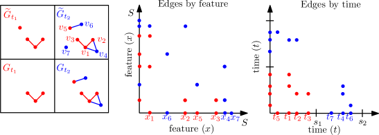
Figure 1: This figure illustrates how we can generate a graphon process $(G_{t})_{t\geq 0}$ from a graphon $\mathcal{W}=(W,\mathscr{S})$, where $\mathscr{S}=(S,\mathcal{S},\mu)$ is a $\sigma$-finite measure space. The two coordinate axes on the middle figure represent our feature space $S$, where the red (resp. blue) dots on the axes represent vertices born during $[0,s_{1}]$ (resp. $(s_{1},s_{2}]$) for $0<s_{1}<s_{2}$, and the red (resp. blue) dots in the interior of the first quadrant represent edges in $G_{t}$ for $t\geq s_{1}$ (resp. $t\geq s_{2}$). The graph $G_{t}$ is an induced subgraph of a graph $\widetilde{G}_{t}$ with infinitely many vertices in the case $\mu(S)=\infty$, such that $G_{t}$ is obtained from $\widetilde{G}_{t}$ by removing isolated vertices. At time $t\geq 0$ the marginal law of the features of $V(\widetilde{G}_{t})$ is a Poisson point process on $S$ with intensity $t\mu$. Two distinct vertices with features $x$ and $x^{\prime}$, respectively, are connected to each other by an undirected edge with probability $W(x,x^{\prime})$. The coordinate axes on the right figure represent time $\mathbb{R}_{+}$. We get the graph $G_{t}$ by considering the edges restricted to $[0,t]^{2}$. Note that the coordinate axes in the right figure and the graphs $\widetilde{G}_{t}$ in the left figure are slightly inaccurate if we assume $\mu(S)=\infty$, since in this case there are infinitely many isolated vertices in $\widetilde{G}_{t}$ for each $t>0$. We have chosen to label the vertices by the order in which they appear in $G_{t}$, where ties are resolved by considering the time the vertices were born, i.e., by considering the time they appeared in $\widetilde{G}_{t}$.

To interpret the graphon process $(G_{t})_{t\geq 0}$ as a family of growing graphs we will need to couple the graphs $G_{t}$ for different times $t\geq 0$. To this end, we consider a Poisson point process $\Gamma$ on $\mathbb{R}_{+}\times S$ (with $\mathbb{R}_{+}:=[0,\infty)$ being equipped with the Borel $\sigma$-algebra and Lebesgue measure). Each point $v=(t,x)$ of $\Gamma$ corresponds to a vertex of an infinite graph $\widetilde{G}$, where the coordinate $t$ is interpreted as the time the vertex is born and the coordinate $x$ describes a feature of the vertex. Two distinct vertices $v=(t,x)$ and $v^{\prime}=(t^{\prime},x^{\prime})$ are connected by an undirected edge with probability $W(x,x^{\prime})$, independently for each possible pair of distinct vertices. For each fixed time $t\geq 0$ define a graph $G_{t}$ by considering the induced subgraph of $\widetilde{G}$ corresponding to vertices which are born at time $t$ or earlier, where we do not include vertices which would be isolated in $G_{t}$. See Figure 1 for an illustration. The family of growing graphs $(G_{t})_{t\geq 0}$ just described includes classical dense $\mathcal{W}$-random graphs (up to isolated vertices) and the sparse graphs studied by Caron and Fox (2014) and Herlau, Schmidt, and Mørup (2016) as special cases, and is (except for minor technical differences) identical to the family of random graphs studied by Veitch and Roy (2015), a paper which was written in parallel with our paper; see our remark at the end of this introduction.

The graphon process $(\widetilde{G}_{t})_{t\geq 0}$ satisfies a natural notion of exchangeability. Roughly speaking, in our setting this means that the features of newly born vertices are homogeneous in time. More precisely, it can be defined as joint exchangeability of a random measure in $\mathbb{R}_{+}^{2}$, where the two coordinates correspond to time, and each edge of the graph corresponds to a point mass. We will prove that graphon processes as defined above, with $W$ integrable and possibly random, are characterized by exchangeability of the random measure in $\mathbb{R}_{+}^{2}$ along with a certain regularity condition we call uniform regularity of tails. See Proposition 26 in Section 2.4. This result is an analogue in the setting of possibly sparse graphs satisfying the aforementioned regularity condition of the Aldous-Hoover theorem (Aldous, 1981; Hoover, 1979), which characterizes $\mathcal{W}$-random graphs over probability spaces as graphs that are invariant in law under permutation of their vertices.

The graphon processes defined above also have a number of other properties making them particularly natural to model sparse graphs or networks. They are suitable for modelling networks which grow over time since no additional rescaling parameters (like the explicitly given density dependence on the number of vertices specified by Bollobás and Riordan, 2009, and Borgs, Chayes, Cohn, and Zhao, 2014a) are necessary; all information about the random graph model is encoded by the graphon alone. The graphs are projective in the sense that if $s<t$ the graph $G_{s}$ is an induced subgraph of $G_{t}$. Finally, a closely related family of weighted graphs is proven by Caron and Fox (2014) to have power law degree distribution for certain $\mathcal{W}$, and our graphon processes are expected to behave similarly. The graphon processes studied in this paper have a different qualitative behavior than the sparse $\mathcal{W}$-random graphs studied by Bollobás and Riordan (2009) and Borgs, Chayes, Cohn, and Zhao (2014a, b) (see Figure 2), with the only overlap of the two theories occurring when the graphs are dense. If the sparsity of the graphs is caused by the degrees of the vertices being scaled down approximately uniformly over time, then the model studied by Bollobás and Riordan (2009) and Borgs, Chayes, Cohn, and Zhao (2014a, b) is most natural. If the sparsity is caused by later vertices typically having lower connectivity probabilities than earlier vertices, then the model presented in this paper is most natural. The sampling method we will use in our forthcoming paper (Borgs, Chayes, Cohn, and Holden, 2017) generalizes both of these methods.

Figure 2: The adjacency matrices of graphs sampled as described by Borgs, Chayes, Cohn, and Zhao (2014a) (left) and in this paper (right), where we used the graphon $\mathcal{W}_{1}=(W_{1},[0,1])$ (left) and the graphon $\mathcal{W}_{2}=(W_{2},\mathbb{R}_{+})$ (right), with $W_{1}(x_{1},x_{2})=x_{1}^{-1/2}x_{2}^{-1/2}$ for $x_{1},x_{2}\in[0,1]$ and $W_{2}(x_{1},x_{2})=\min(0.8,7\min(1,x_{1}^{-2})\min(1,x_{2}^{-2}))$ for $x_{1},x_{2}\in\mathbb{R}_{+}$. Black (resp. white) indicates that there is (resp. is not) an edge. We rescaled the height of the graphon by $\rho:=1/40$ on the left figure. As described by Borgs, Chayes, Cohn, and Zhao (2014a, b) the type of each vertex is sampled independently and uniformly from $[0,1]$, and each pair of vertices is connected with probability $\min(\rho W_{1},1)$. In the right figure the vertices were sampled by a Poisson point process on $\mathbb{R}_{+}$ of intensity $t=4$, and two vertices were connected independently with a probability given by $W_{2}$; see Section 2.4 and the main text of this introduction. The two graphs have very different qualitative properties. In the left graph most vertices have a degree close to the average degree, where the average degree depends on our scaling factor $\rho$. In the right graph the edges are distributed more inhomogeneously: most of the edges are contained in induced subgraphs of constant density, and the sparsity is caused by a large number of vertices with very low degree.

To compare different models, and to discuss notions of convergence, we introduce the following natural generalization of the cut metric for graphons on probability spaces to our setting. For two graphons $\mathcal{W}_{1}=(W_{1},\mathscr{S}_{1})$ and $\mathcal{W}_{2}=(W_{2},\mathscr{S}_{2})$, this metric is easiest to define when the two graphons are defined over the same space. However, for applications we want to compare graphons over different spaces, say two Borel spaces $\mathscr{S}_{1}$ and $\mathscr{S}_{2}$. Assuming that both Borel spaces have infinite total measure, the cut distance between $\mathcal{W}_{1}$ and $\mathcal{W}_{2}$ can then be defined as

$$\delta_{\square}(\mathcal{W}_{1},\mathcal{W}_{2})=\inf_{\psi_{1},\psi_{2}}\sup_{U,V\subseteq\mathbb{R}_{+}^{2}}\left|\int_{U\times V}\big{(}W_{1}^{\psi_{1}}-W_{2}^{\psi_{2}}\big{)}\,d\mu\,d\mu\right|,$$ (1)

where we take the infimum over measure-preserving maps $\psi_{j}\colon\mathbb{R}_{+}\to S_{j}$ for $j=1,2$, $W_{j}^{\psi_{j}}(x,y):=W_{j}(\psi_{j}(x),\psi_{j}(y))$ for $x,y\in\mathbb{R}_{+}$, and the supremum is over measurable sets $U,V\subseteq\mathbb{R}_{+}^{2}$. (See Definition 5 below for the definition of the cut distance for graphons over general spaces, including the case where one or both spaces have finite total mass.) We call two graphons equivalent if they have cut distance zero. As we will see, two graphons are equivalent if and only if the random families $(G_{t})_{t\geq 0}$ generated from these graphons have the same distribution; see Theorem 27 below.

To compare graphs and graphons, we embed a graph on $n$ vertices into the set of step functions over $[0,1]^{2}$ in the usual way by decomposing $[0,1]$ into adjacent intervals $I_{1},\dots,I_{n}$ of lengths $1/n$, and define a step function $W^{G}$ as the function which is equal to $1$ on $I_{i}\times I_{j}$ if $i$ and $j$ are connected in $G$, and equal to $0$ otherwise. Extending $W^{G}$ to a function on $\mathbb{R}_{+}^{2}$ by setting it to zero outside of $[0,1]^{2}$, we can then compare graphs to graphons on measure spaces of infinite mass, and in particular we get a notion of convergence in metric of a sequence of graphs $(G_{n})_{n\in\mathbb{N}}$ to a graphon $\mathcal{W}$.

In the classical theory of graph convergence, such a sequence will converge to the zero graphon whenever the sequence is sparse. We resolve this difficulty by rescaling the input arguments of the step function $W^{G}$ so as to get a “stretched graphon” $\mathcal{W}^{G,s}=(W^{G,s},\mathbb{R}_{+})$ satisfying $\|W^{G,s}\|_{1}=1$. Equivalently, we may interpret $\mathcal{W}^{G,s}$ as a graphon where the measure of the underlying measure space is rescaled. See Figure 3 for an illustration, which also compares the rescaling in the current paper with the rescaling considered by Borgs, Chayes, Cohn, and Zhao (2014a). We say that $(G_{n})_{n\in\mathbb{N}}$ converges to a graphon $\mathcal{W}$ (with $L^{1}$ norm equal to 1) for the stretched cut metric if $\lim_{n\rightarrow\infty}\delta_{\square}(\mathcal{W}^{G_{n},s},\mathcal{W})=0$. Graphons on $\sigma$-finite measure spaces of infinite total measure may therefore be considered as limiting objects for sequences of sparse graphs, similarly as graphons on probability spaces are considered limits of dense graphs. We prove that graphon processes converge to the generating graphon in the stretched cut metric; see Proposition 28 in Section 2.4. We will also consider another family of random sparse graphs associated with a graphon $\mathcal{W}$ over a $\sigma$-finite measure space, and prove that these graphs are also converging for the stretched cut metric.

Figure 3: The figure shows three graphons associated with the same simple graph $G$ on five vertices. In the classical theory of graphons all simple sparse graphs converge to the zero graphon. We may prevent this by renormalizing the graphons, either by rescaling the height of the graphon (middle) or by stretching the domain on which it is defined (right). The first approach was chosen by Bollobás and Riordan (2009) and Borgs, Chayes, Cohn, and Zhao (2014a, b), and the second approach is chosen in this paper. In our forthcoming paper (Borgs, Chayes, Cohn, and Holden, 2017) we choose a combined approach, where the renormalization depends on the observed graph.

Particular random graph models of special interest arise by considering certain classes of graphons $\mathcal{W}$. Caron and Fox (2014) consider graphons on the form $W(x_{1},x_{2})=1-\exp(-f(x_{1})f(x_{2}))$ (with a slightly different definition on the diagonal, since they also allow for self-edges) for certain decreasing functions $f\colon\mathbb{R}_{+}\to\mathbb{R}_{+}$. In this model $x$ represents a sociability parameter of each vertex. A multi-edge version of this model allows for an alternative sampling procedure to the one we present above (Caron and Fox, 2014, Section 3). Herlau, Schmidt, and Mørup (2016) introduced a generalization of the model of Caron and Fox (2014) to graphs with block structure. In this model each node is associated to a type from a finite index set $[K]:=\{1,\dots,K\}$ for some $K\in\mathbb{N}$, in addition to its sociability parameter, such that the probability of two nodes connecting depends both on their type and their sociability. More generally we can obtain sparse graphs with block structure by considering integrable functions $W_{k_{1},k_{2}}\colon\mathbb{R}_{+}^{2}\to[0,1]$ for $k_{1},k_{2}\in\{1,\dots,K\}$, and defining $S:=[K]\times\mathbb{R}_{+}$ and $W((k_{1},x_{1}),(k_{2},x_{2})):=W_{k_{1},k_{2}}(x_{1},x_{2})$. As compared to the block model of Herlau, Schmidt, and Mørup (2016), this allows for a more complex interaction within and between the blocks. An alternative generalization of the stochastic block model to our setting is to consider infinitely many disjoint intervals $I_{k}\subset\mathbb{R}_{+}$ for $k\in\mathbb{N}$, and define $W:=\sum_{k_{1},k_{2}\in\mathbb{N}}p_{k_{1},k_{2}}\mathbf{1}_{I_{k_{1}}\times I_{k_{2}}}$ for constants $p_{k_{1},k_{2}}\in[0,1]$. For the block model of Herlau, Schmidt, and Mørup (2016) and our first generalization above (with $S:=[K]\times\mathbb{R}_{+}$), the degree distribution of the vertices within each block will typically be strongly inhomogeneous; by contrast, in our second generalization above (with infinitely many blocks), all vertices within the same block have the same connectivity probabilities, and hence the degree distribution will be more homogeneous.

We can also model sparse graphs with mixed membership structure within our framework. In this case we let $\widetilde{S}\subset[0,1]^{K}$ be the standard $(K-1)$-simplex, and define $S:=\widetilde{S}\times\mathbb{R}_{+}$. For a vertex with feature $(\widetilde{x},x)\in\widetilde{S}\times\mathbb{R}_{+}$ the first coordinate $\widetilde{x}=(\widetilde{x}_{1},\dots,\widetilde{x}_{K})$ is a vector such that $\widetilde{x}_{j}$ for $j\in[K]$ describes the proportion of time the vertex is part of community $j\in[K]$, and the second coordinate $x$ describes the role of the vertex within the community; for example, $x$ could be a sociability parameter. For each $k_{1},k_{2}\in[K]$ let $\mathcal{W}_{k_{1},k_{2}}=(W_{k_{1},k_{2}},\mathbb{R}_{+})$ be a graphon describing the interactions between the communities $k_{1}$ and $k_{2}$. We define our mixed membership graphon $\mathcal{W}=(W,\mathscr{S})$ by

$$W\big{(}(\widetilde{x}^{1},x^{1}),(\widetilde{x}^{2},x^{2})\big{)}:=\sum_{k_{1},k_{2}\in[K]}\widetilde{x}^{1}_{k_{1}}\widetilde{x}^{2}_{k_{2}}W_{k_{1},k_{2}}(x^{1},x^{2}).$$

Alternatively, we could define $S:=\widetilde{S}\times\mathbb{R}_{+}^{K}$, which would provide a model where, for example, the sociability of a node varies depending on which community it is part of.

In the classical setting of dense graphs, many papers only consider graphons defined on the unit square, instead of graphons on more general probability spaces. This is justified by the fact that every graphon with a probability space as base space is equivalent to a graphon with base space $[0,1]$. The analogue in our setting would be graphons over $\mathbb{R}_{+}$ equipped with the Lebesgue measure. As the examples in the preceding paragraphs illustrate, for certain random graph models it is more natural to consider another underlying measure space. For example, each coordinate in some higher-dimensional space may correspond to a particular feature of the vertices, and changing the base space can disrupt certain properties of the graphon, such as smoothness conditions. For this reason we consider graphons defined on general $\sigma$-finite measure spaces in this paper. However, we will prove that every graphon is equivalent to a graphon on $\mathbb{R}_{+}$ equipped with the Borel $\sigma$-algebra and Lebesgue measure, in the sense that their cut distance is zero; see Proposition 10 in Section 2.2. As stated before, our results then imply that they correspond to the same random graph model.

The set of $[0,1]$-valued graphons on probability spaces is compact for the cut metric. For the possibly unbounded graphons studied by Borgs, Chayes, Cohn, and Zhao (2014a), which are real-valued and defined on probability spaces, compactness holds if we consider closed subsets of the space of graphons which are uniformly upper regular (see Section 2.3 for the definition). In our setting, where we look at graphons over spaces of possibly infinite measure, the analogous regularity condition is uniform regularity of tails if we restrict ourselves to, say, $[0,1]$-valued graphons. In particular our results imply that a sequence of simple graphs with uniformly regular tails is subsequentially convergent, and conversely, that every convergent sequence of simple graphs has uniformly regular tails. See Theorem 15 in Section 2.3 and the two corollaries following this theorem.

In the setting of dense graphs, convergence for the cut metric is equivalent to left convergence, meaning that subgraph densities converge. This equivalence does not hold in our setting, or for the unbounded graphons studied by Borgs, Chayes, Cohn, and Zhao (2014a, b); its failure is characteristic of sparse graphs, because deleting even a tiny fraction of the edges in a sparse graph can radically change the densities of larger subgraphs (see the discussion by Borgs, Chayes, Cohn, and Zhao, 2014a, Section 2.9). However, randomly sampled graphs do satisfy a notion of left convergence; see Proposition 30 in Section 2.5.

As previously mentioned, in our forthcoming paper (Borgs, Chayes, Cohn, and Holden, 2017) we will generalize and unify the theories and models presented by Bollobás and Riordan (2009), Borgs, Chayes, Cohn, and Zhao (2014a, b), Caron and Fox (2014), Herlau, Schmidt, and Mørup (2016), and Veitch and Roy (2015). Along with the introduction of a generalized model for sampling graphs and an alternative (and weaker) cut metric, we will prove a number of convergence properties of these graphs. Since the graphs in this paper are obtained as a special case of the graphs in our forthcoming paper, the mentioned convergence results also hold in our setting.

In Section 2 we will state the main results of this paper, which will be proved in the subsequent appendices. In Appendix A we prove that the cut metric $\delta_{\square}$ is well defined. In Appendix B we prove that any graphon is equivalent to a graphon with underlying measure space $\mathbb{R}_{+}$. We also prove that under certain conditions on the underlying measure space we may define the cut metric $\delta_{\square}$ in a number of equivalent ways. In Appendix C, we deal with some technicalities regarding graph-valued processes. In Appendix D we prove that certain random graph models derived from a graphon $\mathcal{W}$, including the graphon processes defined above, give graphs converging to $\mathcal{W}$ for the cut metric. We also prove that two graphons are equivalent (i.e., they have cut distance zero) iff the corresponding graphon processes are equal in law. In Appendix E we prove that uniform regularity of tails is sufficient to guarantee subsequential metric convergence for a sequence of graphs; conversely, we prove that every convergent sequence of graphs with non-negative edge weights has uniformly regular tails. In Appendix F we prove some basic properties of sequences of graphs which are metric convergent, for example that metric convergence implies unbounded average degree if the number of edges diverge and the graph does not have too many isolated vertices; see Proposition 22 below. We also compare the notion of metric graph convergence in this paper to the one studied by Borgs, Chayes, Cohn, and Zhao (2014a). In Appendix G we prove with reference to the Kallenberg theorem for jointly exchangeable measures that graphon processes for integrable $W$ are uniquely characterized as exchangeable graph processes satisfying uniform tail regularity. We also describe more general families of graphs that may be obtained from the Kallenberg representation theorem if this regularity condition is not imposed. Finally, in Appendix H we prove our results on left convergence of graphon processes.

Remark 1

After writing a first draft of this work, but a little over a month before completing the paper, we became aware of parallel, independent work by Veitch and Roy (2015), who introduce a closely related model for exchangeable sparse graphs and interpret it with reference to the Kallenberg theorem for exchangeable measures. The random graph model studied by Veitch and Roy (2015) is (up to minor differences) the same as the graphon processes introduced in the current paper. Aside from both introducing this model, the results of the two papers are essentially disjoint. While Veitch and Roy (2015) focus on particular properties of the graphs in a graphon process (in particular, the expected number of edges and vertices, the degree distribution, and the existence of a giant component under certain assumptions on $\mathcal{W}$), our focus is graph convergence, the cut metric, and the question of when two different graphons lead to the same graphon process.

See also the subsequent paper by Janson (2016) expanding on the results of our paper, characterizing in particular when two graphons are equivalent, and proving additional compactness results for graphons over $\sigma$-finite spaces.

2 Definitions and Main Results

We will work mainly with simple graphs, but we will allow the graphs to have weighted vertices and edges for some of our definitions and results. We denote the vertex set of a graph $G$ by $V(G)$ and the edge set of $G$ by $E(G)$. The sets $V(G)$ and $E(G)$ may be infinite, but we require them to be countable. If $G$ is weighted, with edge weights $\beta_{ij}(G)$ and vertex weights $\alpha_{i}(G)$, we require the vertex weights to be non-negative, and we often (but not always) require that $\|\beta(G)\|_{1}:=\sum_{i,j\in V(G)}\alpha_{i}(G)\alpha_{j}(G)|\beta_{ij}(G)|<\infty$ (note that $\|\beta(G)\|_{1}$ is defined in such a way that for an unweighted graph, it is equal to $2|E(G)|$, as opposed to the density, which is ill-defined if $|V(G)|=\infty$). We define the edge density of a finite simple graph $G$ to be $\rho(G):=2|E(G)|/|V(G)|^{2}$. Letting $\mathbb{N}=\{1,2,\dots\}$ denote the positive integers, a sequence $(G_{n})_{n\in\mathbb{N}}$ of simple, finite graphs will be called sparse if $\rho(G_{n})\to 0$ as $n\to\infty$, and dense if $\liminf_{n\to\infty}\rho(G_{n})>0$. When we consider graph-valued stochastic processes $(G_{n})_{n\in\mathbb{N}}$ or $(G_{t})_{t\geq 0}$ of simple graphs, we will assume each vertex is labeled by a distinct number in $\mathbb{N}$, so we can view $V(G)$ as a subset of $\mathbb{N}$ and $E(G)$ as a subset of $\mathbb{N}\times\mathbb{N}$. The labels allow us to keep track of individual vertices in the graph over time. In Section 2.4 we define a topology and $\sigma$-algebra on the set of such graphs.

2.1 Measure-theoretic Preliminaries

We start by recalling several notions from measure theory.

For two measure spaces $\mathscr{S}=(S,\mathcal{S},\mu)$ and $\mathscr{S}^{\prime}=(S^{\prime},\mathcal{S}^{\prime},\mu^{\prime})$, a measurable map $\phi\colon S\to S^{\prime}$ is called measure-preserving if for every $A\in\mathcal{S}^{\prime}$ we have $\mu(\phi^{-1}(A))=\mu^{\prime}(A)$. Two measure spaces $(S,\mathcal{S},\mu)$ and $(S^{\prime},\mathcal{S}^{\prime},\mu^{\prime})$ are called isomorphic if there exists a bimeasurable, bijective, and measure-preserving map $\phi\colon S\to S^{\prime}$. A Borel measure space is defined as a measure space that is isomorphic to a Borel subset of a complete separable metric space equipped with a Borel measure.

Throughout most of this paper, we consider $\sigma$-finite measure spaces, i.e., spaces $\mathscr{S}=(S,\mathcal{S},\mu)$ such that $S$ can be written as a countable union of sets $A_{i}\in\mathcal{S}$ with $\mu(A_{i})<\infty$. Recall that a set $A\in\mathcal{S}$ is an atom if $\mu(A)>0$ and if every measurable $B\subseteq A$ satisfies either $\mu(B)=0$ or $\mu(B)=\mu(A)$. The measure space $\mathscr{S}$ is atomless if it has no atoms. Every atomless $\sigma$-finite Borel space of infinite measure is isomorphic to $(\mathbb{R}_{+},\mathcal{B},\lambda)$, where $\mathcal{B}$ is the Borel $\sigma$-algebra and $\lambda$ is Lebesgue measure; for the convenience of the reader, we prove this as Lemma 33 below.

We also need the notion of a coupling, a concept well known for probability spaces: if $(S_{i},\mathcal{S}_{i},\mu_{i})$ is a measure space for $i=1,2$ and $\mu_{1}(S_{1})=\mu_{2}(S_{2})\in(0,\infty]$, we say that $\mu$ is a coupling of $\mu_{1}$ and $\mu_{2}$ if $\mu$ is a measure on $(S_{1}\times S_{2},\mathcal{S}_{1}\times\mathcal{S}_{2})$ with marginals $\mu_{1}$ and $\mu_{2}$, i.e., if $\mu(U\times S_{2})=\mu_{1}(U)$ for all $U\in\mathcal{S}_{1}$ and $\mu(S_{1}\times U)=\mu_{2}(U)$ for all $U\in\mathcal{S}_{2}$. Note that this definition of coupling is closely related to the definition of coupling of probability measures, which applies when $\mu_{1}(S_{1})=\mu_{2}(S_{2})=1$. For probability spaces, it is easy to see that every pair of measures has a coupling (for example, the product space of the two probability spaces). We prove the existence of a coupling for $\sigma$-finite measure spaces in Appendix A, where this fact is stated as part of a more general lemma, Lemma 34.

Finally, we say that a measure space $\widetilde{\mathscr{S}}=(\widetilde{S},\widetilde{\mathcal{S}},\widetilde{\mu})$ extends a measure space $\mathscr{S}=(S,\mathcal{S},\mu)$ if $S\in\widetilde{\mathcal{S}}$, $\mathcal{S}=\{A\cap S\,:\,A\in\widetilde{\mathcal{S}}\}$, and $\mu(A)=\widetilde{\mu}(A)$ for all $A\in\mathcal{S}$. We say that $\mathscr{S}$ is a restriction of $\widetilde{\mathscr{S}}$, or, if $S$ is specified, the restriction of $\widetilde{\mathscr{S}}$ to $S$.

2.2 Graphons and Cut Metric

We will work with the following definition of a graphon.

Definition 2

A graphon is a pair $\mathcal{W}=(W,\mathscr{S})$, where $\mathscr{S}=(S,\mathcal{S},\mu)$ is a $\sigma$-finite measure space satisfying $\mu(S)>0$ and $W$ is a symmetric real-valued function $W\in L^{1}(S\times S)$ that is measurable with respect to the product $\sigma$-algebra $\mathcal{S}\times\mathcal{S}$ and integrable with respect to $\mu\times\mu$. We say that $\mathcal{W}$ is a graphon over $\mathscr{S}$.

Remark 3

Most literature on graphons defines a graphon to be the function $W$ instead of the pair $(W,\mathscr{S})$. We have chosen the above definition since the underlying measure space will play an important role. Much literature on graphons requires $W$ to take values in $[0,1]$, and some of our results will also be restricted to this case. The major difference between the above definition and the definition of a graphon in the existing literature, however, is that we allow the graphon to be defined on a measure space of possibly infinite measure, instead of a probability space.

Remark 4

One may relax the integrability condition for $W$ in the above definition such that the corresponding random graph model (as defined in Definition 25 below) still gives graphs with finitely many vertices and edges for each bounded time. This more general definition is used by Veitch and Roy (2015). We work with the above definition since the majority of the analysis in this paper is related to convergence properties and graph limits, and our definition of the cut metric is most natural for integrable graphons. An exception is the notion of subgraph density convergence in the corresponding random graph model, which we discuss in the more general setting of not necessarily integrable graphons; see Remark 31 below.

We will mainly study simple graphs in the current paper, in particular, graphs which do not have self-edges. However, the theory can be generalized in a straightforward way to graphs with self-edges, in which case we would also impose an integrability condition for $W$ along its diagonal.

If $\mathcal{W}=(W,(S,\mathcal{B},\lambda))$, where $S$ is a Borel subset of $\mathbb{R}$, $\mathcal{B}$ is the Borel $\sigma$-algebra, and $\lambda$ is Lebesgue measure, we write $\mathcal{W}=(W,S)$ to simplify notation. For example, we write $\mathcal{W}=(W,\mathbb{R}_{+})$ instead of $\mathcal{W}=(W,(\mathbb{R}_{+},\mathcal{B},\lambda))$.

For any measure space $\mathscr{S}=(S,\mathcal{S},\mu)$ and integrable function $W\colon S\times S\to\mathbb{R}$, define the cut norm of $W$ over $\mathscr{S}$ by

$$\|W\|_{\square,S,\mu}:=\sup_{U,V\in\mathcal{S}}\left|\int_{U\times V}W(x,y)\,d\mu(x)\,d\mu(y)\right|.$$

If $S$ and/or $\mu$ is clear from the context we may write $\|\cdot\|_{\square}$ or $\|\cdot\|_{\square,\mu}$ to simplify notation.

Given a graphon $\widetilde{\mathcal{W}}=(\widetilde{W},\widetilde{\mathscr{S}})$ with $\widetilde{\mathscr{S}}=(\widetilde{S},\widetilde{\mathcal{S}},\widetilde{\mu})$ and a set $S\in\widetilde{\mathcal{S}}$, we say that $\mathcal{W}=(W,\mathscr{S})$ is the restriction of $\widetilde{\mathcal{W}}$ to $S$ if $\mathscr{S}$ is the restriction of $\widetilde{\mathscr{S}}$ to $S$ and $\widetilde{W}|_{S\times S}=W$. We say that $\widetilde{\mathcal{W}}=(\widetilde{W},\widetilde{\mathscr{S}})$ is the trivial extension of $\mathcal{W}$ to $\widetilde{\mathscr{S}}$ if $\mathcal{W}=(W,\mathscr{S})$ is the restriction of $\widetilde{\mathcal{W}}$ to $S$ and $\operatorname{supp}(\widetilde{W})\subseteq S\times S$. For measure spaces $\mathscr{S}=(S,\mathcal{S},\mu)$ and $\mathscr{S}^{\prime}=(S^{\prime},\mathcal{S}^{\prime},\mu^{\prime})$, a graphon $\mathcal{W}=(W,\mathscr{S})$, and a measurable map $\phi\colon S^{\prime}\to S$, we define the graphon $\mathcal{W}^{\phi}=(W^{\phi},\mathscr{S}^{\prime})$ by $W^{\phi}(x_{1},x_{2}):=W(\phi(x_{1}),\phi(x_{2}))$ for $x_{1},x_{2}\in S^{\prime}$. We say that $\mathcal{W}^{\phi}$ (resp. $W^{\phi}$) is a pullback of $\mathcal{W}$ (resp. $W$) onto $\mathscr{S^{\prime}}$. Finally, let $\|\cdot\|_{1}$ denote the $L^{1}$ norm.

Definition 5

For $i=1,2$, let $\mathcal{W}_{i}=(W_{i},\mathscr{S}_{i})$ with $\mathscr{S}_{i}=(S_{i},\mathcal{S}_{i},\mu_{i})$ be a graphon.

• If $\mu_{1}(S_{1})=\mu_{2}(S_{2})\in(0,\infty]$, the cut metric $\delta_{\square}$ and invariant $L^{1}$ metric $\delta_{1}$ are defined by

  $$\begin{split}\delta_{\square}(\mathcal{W}_{1},\mathcal{W}_{2})&:=\inf_{\mu}\|W_{1}^{\pi_{1}}-W_{2}^{\pi_{2}}\|_{\square,S_{1}\times S_{2},\mu}\quad\text{and}\\ \delta_{1}(\mathcal{W}_{1},\mathcal{W}_{2})&:=\inf_{\mu}\|W_{1}^{\pi_{1}}-W_{2}^{\pi_{2}}\|_{1,S_{1}\times S_{2},\mu},\end{split}$$ (2)

  where $\pi_{i}\colon S_{1}\times S_{2}\to S_{i}$ denotes projection for $i=1,2$, and we take the infimum over all couplings $\mu$ of $\mu_{1}$ and $\mu_{2}$.

• If $\mu_{1}(S_{1})\neq\mu_{2}(S_{2})$, let $\widetilde{\mathscr{S}}_{i}=(\widetilde{S}_{i},\widetilde{\mathcal{S}}_{i},\widetilde{\mu}_{i})$ be a $\sigma$-finite measure space extending $\mathscr{S}_{i}$ for $i=1,2$ such that $\widetilde{\mu}_{1}(\widetilde{S}_{1})=\widetilde{\mu}_{2}(\widetilde{S}_{2})\in(0,\infty]$. Let $\widetilde{\mathcal{W}}_{i}=(\widetilde{W}_{i},\widetilde{\mathscr{S}}_{i})$ be the trivial extension of $\mathcal{W}_{i}$ to $\widetilde{\mathscr{S}}_{i}$, and define

  $$\delta_{\square}(\mathcal{W}_{1},\mathcal{W}_{2}):=\delta_{\square}(\widetilde{\mathcal{W}}_{1},\widetilde{\mathcal{W}}_{2})\quad\text{and}\quad\delta_{1}(\mathcal{W}_{1},\mathcal{W}_{2}):=\delta_{1}(\widetilde{\mathcal{W}}_{1},\widetilde{\mathcal{W}}_{2}).$$

• We call two graphons $\mathcal{W}_{1}$ and $\mathcal{W}_{2}$ equivalent if $\delta_{\square}(\mathcal{W}_{1},\mathcal{W}_{2})=0$.

The following proposition will be proved in Appendix A. Recall that a pseudometric on a set $S$ is a function from $S\times S$ to $\mathbb{R}_{+}$ which satisfies all the requirements of a metric, except that the distance between two different points might be zero.

Proposition 6

The metrics $\delta_{\square}$ and $\delta_{1}$ given in Definition 5 are well defined; in other words, under the assumptions of (i) there exists at least one coupling $\mu$, and under the assumptions of (ii) the definitions of $\delta_{\square}(\mathcal{W}_{1},\mathcal{W}_{2})$ and $\delta_{\mathbf{1}}(\mathcal{W}_{1},\mathcal{W}_{2})$ do not depend on the choice of extensions $\widetilde{\mathscr{S}}_{1},\widetilde{\mathscr{S}}_{2}$. Furthermore, $\delta_{\square}$ and $\delta_{1}$ are pseudometrics on the space of graphons.

An important input to the proof of the proposition (Lemma 42 in Appendix A) is that the $\delta_{\square}$ (resp. $\delta_{1}$) distance between two graphons over spaces of equal measure, as defined in Definition 5(i), is invariant under trivial extensions. The lemma is proved by first showing that it holds for step functions (where the proof more or less boils down to an explicit calculation) and then using the fact that every graphon can be approximated by a step function.

We will see in Proposition 48 in Appendix B that under additional assumptions on the underlying measure spaces $\mathscr{S}_{1}$ and $\mathscr{S}_{2}$ the cut metric can be defined equivalently in a number of other ways, giving, in particular, the equivalence of the definitions (1) and (2) in the case of two Borel spaces of infinite mass. Similar results hold for the metric $\delta_{1}$; see Remark 49.

While the two metrics $\delta_{\square}$ and $\delta_{1}$ are not equivalent, a fact which is already well known from the theory of graph convergence for dense graphs, it turns out that the statement that two graphons have distance zero in the cut metric is equivalent to the same statement in the invariant $L^{1}$ metric. This is the content of our next proposition.

Proposition 7

Let $\mathcal{W}_{1}$ and $\mathcal{W}_{2}$ be graphons. Then $\delta_{\square}(\mathcal{W}_{1},\mathcal{W}_{2})=0$ if and only if $\delta_{1}(\mathcal{W}_{1},\mathcal{W}_{2})=0$.

The proposition will be proved in Appendix B. (We will actually prove a generalization of this proposition involving an invariant version of the $L^{p}$ metric; see Proposition 50.) The proof proceeds by first showing (Proposition 51) that if $\delta_{\square}(\mathcal{W}_{1},\mathcal{W}_{2})=0$ for graphons $\mathcal{W}_{i}=(W_{i},\mathscr{S}_{i})$ with $\mathscr{S}_{i}=(S_{i},\mathcal{S}_{i},\mu_{i})$ for $i=1,2$, then there exists a particular measure $\mu$ on $S_{1}\times S_{2}$ such that $\|W_{1}^{\pi_{1}}-W^{\pi_{2}}_{2}\|_{\square,\mu}=0$. Under certain conditions we may assume that $\mu$ is a coupling measure, in which case it follows that the infimum in the definition of $\delta_{\square}$ is a minimum; see Proposition 8 below.

To state our next proposition we define a coupling between two graphons $\mathcal{W}_{i}=(W_{i},\mathscr{S}_{i})$ with $\mathscr{S}_{i}=(S_{i},\mathcal{S}_{i},\mu_{i})$ for $i=1,2$ as a pair of graphons $\widetilde{\mathcal{W}}_{i}$ over a space of the form $\mathscr{S}=(S_{1}\times S_{2},\mathcal{S}_{1}\times\mathcal{S}_{2},\mu)$, where $\mu$ is a coupling of $\mu_{1}$ and $\mu_{2}$ and $\widetilde{\mathcal{W}}_{i}=W_{i}^{\pi_{i}}$, and where as before, $\pi_{i}$ denotes the projection from $S_{1}\times S_{2}$ onto $S_{i}$ for $i=1,2$.

Proposition 8

Let $\mathcal{W}_{i}$ be graphons over $\sigma$-finite Borel spaces $\mathscr{S}_{i}=(S_{i},\mathcal{S}_{i},\mu_{i})$, and let $\widetilde{S}_{i}=\{x\in S_{i}\colon\int|W_{i}(x,y)|d\mu_{i}(y)>0\}$, for $i=1,2$. If $\delta_{\square}(\mathcal{W}_{1},\mathcal{W}_{2})=0$, then the restrictions of $\mathcal{W}_{1}$ and $\mathcal{W}_{2}$ to $\widetilde{S}_{1}$ and $\widetilde{S}_{2}$ can be coupled in such a way that they are equal a.e.

The proposition will be proved in Appendix B. Note that Janson (2016, Theorem 5.3) independently proved a similar result, building on a previous version of the present paper which did not yet contain Proposition 8. His result states that if the cut distance between two graphons over $\sigma$-finite Borel spaces is zero, then there are trivial extensions of these graphons such that the extensions can be coupled so as to be equal almost everywhere. It is easy to see that our result implies his, but we believe that with a little more work, it should be possible to deduce ours from his as well.

Remark 9

Note that the classical theory of graphons on probability spaces appears as a special case of the above definitions by taking $\mathscr{S}$ to be a probability space. Our definition of the cut metric $\delta_{\square}$ is equivalent to the standard definition for graphons on probability spaces; see, for example, papers by Borgs, Chayes, Lovász, Sós, and Vesztergombi (2008) and Janson (2013). Note that $\delta_{\square}$ is not a true metric, only a pseudometric, but we call it a metric to be consistent with existing literature on graphons. However, it is a metric on the set of equivalence classes as derived from the equivalence relation in Definition 5 (iii).

We work with graphons defined on general $\sigma$-finite measure spaces, rather than graphons on $\mathbb{R}_{+}$, since particular underlying spaces are more natural to consider for certain random graphs or networks. However, the following proposition shows that every graphon is equivalent to a graphon over $\mathbb{R}_{+}$.

Proposition 10

For each graphon $\mathcal{W}=(W,\mathscr{S})$ there exists a graphon $\mathcal{W}^{\prime}=(W^{\prime},\mathbb{R}_{+})$ such that $\delta_{\square}(\mathcal{W},\mathcal{W}^{\prime})=0$.

The proof of the proposition follows a similar strategy as the proof of the analogous result for probability spaces by Borgs, Chayes, and Lovász (2010, Theorem 3.2) and Janson (2013, Theorem 7.1), and will be given in Appendix B. The proof uses in particular the result that an atomless $\sigma$-finite Borel space is isomorphic to an interval equipped with Lebesgue measure (Lemma 33).

2.3 Graph Convergence

To define graph convergence in the cut metric, one traditionally (Borgs, Chayes, Lovász, Sós, and Vesztergombi, 2006; Lovász and Szegedy, 2006; Borgs, Chayes, Lovász, Sós, and Vesztergombi, 2008) embeds the set of graphs into the set of graphons via the following map. Given any finite weighted graph $G$ we define the canonical graphon $\mathcal{W}^{G}=(W^{G},[0,1])$ as follows. Let $v_{1},\dots,v_{n}$ be an ordering of the vertices of $G$. For any $v_{i}\in V(G)$ let $\alpha_{i}>0$ denote the weight of $v_{i}$, for any $(v_{i},v_{j})\in E(G)$ let $\beta_{ij}\in\mathbb{R}$ denote the weight of the edge $(v_{i},v_{j})$, and for $(v_{i},v_{j})\not\in V(G)$ define $\beta_{ij}=0$. By rescaling the vertex weights if necessary we assume without loss of generality that $\sum_{i=1}^{|V(G)|}\alpha_{i}=1$. If $G$ is simple all vertices have weight $|V(G)|^{-1}$, and we define $\beta_{ij}:=\mathbf{1}_{(v_{i},v_{j})\in E(G)}$. Let $I_{1},\dots,I_{n}$ be a partition of $[0,1]$ into adjacent intervals of lengths $\alpha_{1},\dots,\alpha_{n}$ (say the first one closed, and all others half open), and finally define $W^{G}$ by

$$W^{G}(x_{1},x_{2})=\beta_{ij}\quad\text{if}\quad x_{1}\in I_{i}{\text{ and }}x_{2}\in I_{j}.$$

Note that $W^{G}$ depends on the ordering of the vertices, but that different orderings give graphons with cut distance zero. We define a sequence of weighted, finite graphs $G_{n}$ to be sparse if $\|W^{G_{n}}\|_{1}\rightarrow 0$ as $n\rightarrow\infty$. Note that this generalizes the definition we gave in the very beginning of Section 2 for simple graphs.

A sequence $(G_{n})_{n\in\mathbb{N}}$ of graphs is then defined to be convergent in metric if $\mathcal{W}^{G_{n}}$ is a Cauchy sequence in the metric $\delta_{\square}$, and it is said to be convergent to a graphon $\mathcal{W}$ if $\delta_{\square}(\mathcal{W}^{G_{n}},\mathcal{W})\to 0$. Equivalently, one can define convergence of $(G_{n})_{n\in\mathbb{N}}$ by identifying a weighted graph $G$ with the graphon $(\beta(G),\mathscr{S}_{G})$, where $\mathscr{S}_{G}$ consists of the vertex set $V(G)$ equipped with the probability measure given by the weights $\alpha_{i}$ (or the uniform measure if $G$ has no vertex weights), and $\beta(G)$ is the function that maps $(i,j)\in V(G)\times V(G)$ to $\beta_{ij}(G)$.

In the classical theory of graph convergence a sequence of sparse graphs converges to the trivial graphon with $W\equiv 0$. This follows immediately from the fact that $\delta_{\square}(\mathcal{W}^{G_{n}},0)\leq\|W^{G_{n}}\|_{1}\to 0$ for sparse graphs. To address this problem, Bollobás and Riordan (2009) and Borgs, Chayes, Cohn, and Zhao (2014a) considered the sequence of reweighted graphons $(\mathcal{W}^{G_{n},r})_{n\in\mathbb{N}}$, where $\mathcal{W}^{G,r}:=(W^{G,r},[0,1])$ with $W^{G,r}:=\frac{1}{\|W^{G}\|_{1}}W^{G}$ for any graph $G$, and defined $(G_{n})_{n\in\mathbb{N}}$ to be convergent iff $(\mathcal{W}^{G_{n},r})_{n\in\mathbb{N}}$ is convergent. The theory developed in the current paper considers a different rescaling, namely a rescaling of the arguments of the function $W^{G}$, which, as explained after Definition 11 below, is equivalent to rescaling the measure of the underlying measurable space.

We define the stretched canonical graphon $\mathcal{W}^{G,s}$ to be identical to $\mathcal{W}^{G}$ except that we “stretch” the function $W^{G}$ to a function $W^{G,s}$ such that $\|W^{G,s}\|_{1}=1$. More precisely, $\mathcal{W}^{G,s}:=(W^{G,s},\mathbb{R}_{+})$, where

$$W^{G,s}(x_{1},x_{2}):=\begin{cases}W^{G}\left(\|W^{G}\|_{1}^{1/2}x_{1},\|W^{G}\|_{1}^{1/2}x_{2}\right)&\text{if }0\leq x_{1},x_{2}\leq\|W^{G}\|_{1}^{-1/2},\text{ and}\\ 0&\text{otherwise}.\end{cases}$$

Note that in the case of a simple graph $G$, each node in $V(G)$ corresponds to an interval of length $1/|V(G)|$ in the canonical graphon $\mathcal{W}^{G}$, while it corresponds to an interval of length $1/\sqrt{2|E(G)|}$ in the stretched canonical graphon.

It will sometimes be convenient to define stretched canonical graphons for graphs with infinitely many vertices (but finitely many edges). Our definition of $W^{G}$ makes no sense for simple graphs with infinitely many vertices, because they cannot all be crammed into the unit interval. Instead, given a finite or countably infinite graph $G$ with vertex weights $(\alpha_{i})_{i\in V(G)}$ which do not necessarily sum to $1$ (and may even sum to $\infty$), we define a graphon $\widetilde{\mathcal{W}}^{G}=(\widetilde{W}^{G},\mathbb{R}_{+})$ by setting $\widetilde{W}^{G}(x,y)=\beta_{ij}(G)$ if $(x,y)\in I_{i}\times I_{j}$, and $\widetilde{W}^{G}(x,y)=0$ if there exist no such pair $(i,j)\in V(G)\times V(G)$, with $I_{i}$ being the interval $[a_{i-1},a_{i})$ where we assume the vertices of $G$ have been labeled $1,2,\dots$, and $a_{i}=\sum_{1\leq k\leq i}\alpha_{k}$ for $i=0,1,\dots$. The stretched canonical graphon will then be defined as the graphon $\mathcal{W}^{G,s}:=(W^{G,s},\mathbb{R}_{+})$ with

$$W^{G,s}(x_{1},x_{2}):=\widetilde{W}^{G}\left(\|\widetilde{W}^{G}\|_{1}^{1/2}x_{1},\|\widetilde{W}^{G}\|_{1}^{1/2}x_{2}\right),$$

a definition which can easily be seen to be equivalent to the previous one if $G$ is a finite graph.

Alternatively, one can define a stretched graphon $G^{s}$ as a graphon over $V(G)$ equipped with the measure $\widehat{\mu}_{G}$, where

$$\widehat{\mu}_{G}(A)=\frac{1}{\sqrt{\|\beta(G)\|_{1}}}\sum_{i\in A}\alpha_{i}$$

for any $A\subseteq V(G)$. In the case where $\sum_{i}\alpha_{i}<\infty$, this graphon is obtained from the graphon representing $G$ by rescaling the probability measure

$$\mu_{G}(A)=\frac{1}{\sum_{i\in V(G)}\alpha_{i}}\sum_{i\in A}\alpha_{i}$$

to the measure $\widehat{\mu}_{G}$, while the function $\beta(G)\colon V(G)\times V(G)\to\mathbb{R}$ with $(i,j)\mapsto\beta_{ij}(G)$ is left untouched.

Note that any graphon with underlying measure space $\mathbb{R}_{+}$ can be “stretched” in the same way as $W^{G}$; in other words, given any graphon $\mathcal{W}=(W,\mathbb{R}_{+})$ we may define a graphon $(W^{\phi},\mathbb{R}_{+})$, where $\phi\colon\mathbb{R}_{+}\to\mathbb{R}_{+}$ is defined to be the linear map such that $\|W^{\phi}\|_{1}=1$, except when $\|W\|_{1}=0$, in which case we define the stretched graphon to be $0$. But for graphons over general measure spaces, this rescaling is ill-defined. Instead, we consider a different, but related, notion of rescaling, by rescaling the measure of the underlying space, a notion which is the direct generalization of our definition of the stretched graphon $G^{s}$.

Definition 11

• For two graphons $\mathcal{W}_{i}=(W_{i},\mathscr{S}_{i})$ with $\mathscr{S}_{i}=(S_{i},\mathcal{S}_{i},\mu_{i})$ for $i=1,2$, define the stretched cut metric $\delta_{\square}^{s}$ by

  $$\delta_{\square}^{s}(\mathcal{W}_{1},\mathcal{W}_{2}):=\delta_{\square}(\widehat{\mathcal{W}}_{1},\widehat{\mathcal{W}}_{2}),$$

  where $\widehat{\mathcal{W}}_{i}:=(W_{i},\widehat{\mathscr{S}}_{i})$ with $\widehat{\mathscr{S}}_{i}:=(S_{i},\mathcal{S}_{i},\widehat{\mu}_{i})$ and $\widehat{\mu}_{i}:=\|W_{i}\|_{1}^{-1/2}\mu_{i}$. (In the particular case where $\|W_{i}\|_{1}=0$, we define $\widehat{\mathcal{W}}_{i}:=(0,{\mathscr{S}}_{i})$.) Identifying $G$ with the graphon ${\widetilde{\mathcal{W}}}^{G}$ introduced above, this also defines the stretched distance between two graphs, or a graph and a graphon.

• A sequence of graphs $(G_{n})_{n\in\mathbb{N}}$ or graphons $(\mathcal{W}_{n})_{n\in\mathbb{N}}$ is called convergent in the stretched cut metric if they form a Cauchy sequence for this metric; they are called convergent to a graphon $\mathcal{W}$ for the stretched cut metric if $\delta^{s}_{\square}(G_{n},\mathcal{W})\to 0$ or $\delta^{s}_{\square}(\mathcal{W}_{n},\mathcal{W})\to 0$, respectively.

Note that for the case of graphons over $\mathbb{R}_{+}$, the above notion of convergence is equivalent to the one involving the stretched graphons $\mathcal{W}_{i}^{s}=(W_{i}^{s},\mathbb{R}_{+})$ of $\mathcal{W}_{i}$ defined by

$$W_{i}^{s}(x_{1},x_{2}):=W_{i}\left(\|W_{i}\|_{1}^{1/2}x_{1},\|W_{i}\|_{1}^{1/2}x_{2}\right).$$

To see this, just note that by the obvious coupling between $\lambda$ and $\widehat{\mu_{i}}$, where in this case $\widehat{\mu_{i}}$ is a constant multiple of Lebesgue measure, we have $\delta_{\square}(\mathcal{W}_{i}^{s},\widehat{\mathcal{W}}_{i})=0$, and hence $\delta_{\square}^{s}(\mathcal{W}_{1},\mathcal{W}_{2})=\delta_{\square}(\mathcal{W}_{1}^{s},\mathcal{W}_{2}^{s})$. As a consequence, we have in particular that $\delta_{\square}^{s}(G,G^{\prime})=\delta_{\square}(G^{s},(G^{\prime})^{s})=\delta_{\square}(\mathcal{W}^{G,s},\mathcal{W}^{G^{\prime},s})$ for any two graphs $G$ and $G^{\prime}$. Note also that the stretched cut metric does not distinguish two graphs obtained from each other by deleting isolated vertices, in the sense that

$$\delta_{\square}^{s}(G,G^{\prime})=0$$ (3)

whenever $G$ is obtained from $G^{\prime}$ by removing a set of vertices that have degree $0$ in $G^{\prime}$.

The following basic example illustrates the difference between the notions of convergence in the classical theory of graphons, the approach for sparse graphs taken by Bollobás and Riordan (2009) and Borgs, Chayes, Cohn, and Zhao (2014a), and the approach of the current paper. Proposition 20 below makes this comparison more general.

Example 12

Let $\alpha\in(0,1)$. For any $n\in\mathbb{N}$ let $G_{n}$ be an Erdős-Rényi graph on $n$ vertices with parameter $n^{\alpha-1}$; i.e., each two vertices of the graph are connected independently with probability $n^{\alpha-1}$. Let $\widetilde{G}_{n}$ be a simple graph on $n$ vertices, such that $\lfloor n^{(1+\alpha)/2}\rfloor$ vertices form a complete subgraph, and $n-\lfloor n^{(1+\alpha)/2}\rfloor$ vertices are isolated. Both graph sequences are sparse, and hence their canonical graphons converge to the trivial graphon for which $W\equiv 0$, i.e., $\delta_{\square}(\mathcal{W}^{G_{n}},0),\delta_{\square}(\mathcal{W}^{\widetilde{G}_{n}},0)\rightarrow 0$, where we let 0 denote the mentioned trivial graphon. The sequence $(G_{n})_{n\in\mathbb{N}}$ converges to $\mathcal{W}_{1}:=(\mathbf{1}_{[0,1]^{2}},[0,1])$ with the notion of convergence introduced by Bollobás and Riordan (2009) and Borgs, Chayes, Cohn, and Zhao (2014a), but does not converge for $\delta_{\square}^{s}$. The sequence $(\widetilde{G}_{n})_{n\in\mathbb{N}}$ converges to $\mathcal{W}_{1}$ for the stretched cut metric, i.e., $\delta^{s}_{\square}(\widetilde{G}_{n},\mathcal{W}_{1})=\delta_{\square}(\mathcal{W}^{\widetilde{G}_{n},s},\mathcal{W}_{1})\rightarrow 0$, but it does not converge with the notion of convergence studied by Bollobás and Riordan (2009) and Borgs, Chayes, Cohn, and Zhao (2014a).

The sequence $(\widetilde{G}_{n})_{n\in\mathbb{N}}$ defined above illustrates one of our motivations to introduce the stretched cut metric. One might argue that this sequence of graphs should converge to the same limit as a sequence of complete graphs; however, earlier theories for graph convergence are too sensitive to isolated vertices or vertices with very low degree to accommodate this.

The space of all $[0,1]$-valued graphons over $[0,1]$ is compact under the cut metric (Lovász and Szegedy, 2007). This implies that every sequence of simple graphs is subsequentially convergent to some graphon under $\delta_{\square}$, when we identify a graph $G$ with its canonical graphon $\mathcal{W}^{G}$. Our generalized definition of a graphon, along with the introduction of the stretched canonical graphon $\mathcal{W}^{G,s}$ and the stretched cut metric $\delta_{\square}^{s}$, raises the question of whether a similar result holds in this setting. We will see in Theorem 15 and Corollary 17 below that the answer is yes, provided we restrict ourselves to uniformly bounded graphons and impose a suitable regularity condition; see Definition 13. The sequence $(G_{n})_{n\in\mathbb{N}}$ in Example 12 illustrates that we may not have subsequential convergence when this regularity condition is not satisfied.

Definition 13

Let $\widetilde{\mathscr{W}}$ be a set of uniformly bounded graphons. We say that $\widetilde{\mathscr{W}}$ has uniformly regular tails if for every $\varepsilon>0$ we can find an $M>0$ such that for every $\mathcal{W}=(W,\mathscr{S})\in\widetilde{\mathscr{W}}$ with $\mathscr{S}=(S,\mathcal{S},\mu)$, there exists $U\in\mathcal{S}$ such that $\|W-W\mathbf{1}_{U\times U}\|_{1}<\varepsilon$ and $\mu(U)\leq M$. A set $\mathcal{G}$ of graphs has uniformly regular tails if $\|\beta(G)\|_{1}<\infty$ for all $G\in\mathcal{G}$ and the corresponding set of stretched canonical graphons $\{\mathcal{W}^{G,s}\,:\,G\in\mathcal{G}\}$ has uniformly regular tails.

Remark 14

It is immediate from the definition that a set of simple graphs $\mathcal{G}$ has uniformly regular tails if and only if for each $\varepsilon>0$ we can find $M>0$ such that the following holds. For all $G\in\mathcal{G}$, assuming the vertices of $G$ are labeled by degree (from largest to smallest) with ties resolved in an arbitrary way,

$$\sum_{i\leq\lceil M\sqrt{|E(G)|}\rceil}\operatorname{deg}(i;G)\leq\varepsilon|E(G)|.$$

In Lemma 59 in Appendix F we will prove that for a set of graphs with uniformly regular tails we may assume the sets $U$ in the above definition correspond to sets of vertices. Note that if a collection $\widetilde{\mathscr{W}}$ of graphons has uniformly regular tails, then every collection of graphons which can be derived from $\widetilde{\mathscr{W}}$ by adding a finite number of the graphons to $\widetilde{\mathscr{W}}$ will still have uniformly regular tails. In other words, if $\widetilde{\mathscr{W}},M,\varepsilon$ are such that the conditions of Definition 13 are satisfied for all but finitely many graphons in $\widetilde{\mathscr{W}}$, then the collection $\widetilde{\mathscr{W}}$ has uniformly regular tails.

The following theorem shows that a necessary and sufficient condition for subsequential convergence is the existence of a subsequence with uniformly regular tails.

Theorem 15

Every sequence $(\mathcal{W}_{n})_{n\in\mathbb{N}}$ of uniformly bounded graphons with uniformly regular tails converges subsequentially to some graphon $\mathcal{W}$ for the cut metric $\delta_{\square}$. Moreover, if $\mathcal{W}_{n}$ is non-negative then every $\delta_{\square}$-Cauchy sequence of uniformly bounded, non-negative graphons has uniformly regular tails.

The proof of the theorem will be given in Appendix E. The most challenging part of the proof is to show that uniform regularity of tails implies subsequential convergence. We prove in Lemma 58 that the property of having uniformly regular tails is invariant under certain operations, which allows us to prove subsequential convergence similarly as in the setting of dense graphs, i.e., by approximating the graphons by step functions and using a martingale convergence theorem.

Two immediate corollaries of Theorem 15 are the following results.

Corollary 16

The set of all $[0,1]$-valued graphons is complete for the cut metric $\delta_{\square}$, and hence also for $\delta_{\square}^{s}$.

Corollary 17

Let $(G_{n})_{n\in\mathbb{N}}$ be a sequence of finite graphs with non-negative, uniformly bounded edge weights such that $|E(G_{n})|<\infty$ for each $n\in\mathbb{N}$. Then the following hold:

1. If $(G_{n})_{n\in\mathbb{N}}$ has uniformly regular tails, then $(G_{n})_{n\in\mathbb{N}}$ has a subsequence that converges to some graphon $\mathcal{W}$ in the stretched cut metric.

2. If $(G_{n})_{n\in\mathbb{N}}$ is a $\delta^{s}_{\square}$-Cauchy sequence, then it has uniformly regular tails.

3. If $(G_{n})_{n\in\mathbb{N}}$ is a $\delta^{s}_{\square}$-Cauchy sequence, then it converges to some graphon $\mathcal{W}$ in the stretched cut metric.

The former of the above corollaries makes two assumptions: (i) the graphons are uniformly bounded, and (ii) the graphons are non-negative. We remark that both of these conditions are necessary.

Remark 18

The set of all $\mathbb{R}_{+}$-valued graphons is not complete for the cut metric $\delta_{\square}$; see for example the argument of Borgs, Chayes, Cohn, and Zhao (2014a, Proposition 2.12(b)) for a counterexample. The set of all $[-1,1]$-valued graphons is also not complete, as the following example suggested to us by Svante Janson illustrates. For each $n\in\mathbb{N}$ let $\mathcal{V}_{n}=(V_{n},\mathbb{R}_{+})$ be a $\{-1,1\}$-valued graphon supported in $[n-1,n]^{2}$ satisfying $\|V_{n}\|_{\square}<2^{-n}$ and $\|V_{n}\|_{1}=1$, by defining $\mathcal{V}_{n}$ to be an appropriately rescaled version of a graphon for a sufficiently large Erdős-Rényi random graph with edge density $1/2$. Define $\mathcal{W}_{n}=(W_{n},\mathbb{R}_{+})$ by $W_{n}:=\sum_{k=1}^{n}V_{k}$, and assume there is a graphon $\mathcal{W}=(W,\mathbb{R}_{+})$ such that $\lim_{n\rightarrow\infty}\delta_{\square}(\mathcal{W},\mathcal{W}_{n})=0$. Then we can find a sequence of measure-preserving transformations $(\phi_{n})_{n\in\mathbb{N}}$ with $\phi_{n}\colon\mathbb{R}_{+}\to\mathbb{R}_{+}$, such that $\lim_{n\rightarrow\infty}\|W^{\phi_{n}}-W_{n}\|_{\square}=0$. This implies that $\lim_{n\rightarrow\infty}\|W^{\phi_{n}}\mathbf{1}_{[k-1,k]^{2}}-V_{k}\|_{\square}=0$ for each $k\in\mathbb{N}$. Since $V_{k}$ is a graphon associated with an Erdős-Rényi random graph it is a step graphon. For any intervals $I,J\subseteq\mathbb{R}_{+}$ such that $V_{k}|_{I\times J}=1$ or $V_{k}|_{I\times J}=-1$ we have $\lim_{n\rightarrow\infty}\|(W^{\phi_{n}}\mathbf{1}_{[k-1,k]^{2}}-V_{k})\mathbf{1}_{I\times J}\|_{\square}=0$, so since $W$ takes values in $[-1,1]$ we have $\lim_{n\rightarrow\infty}\|W^{\phi_{n}}\|_{L^{1}(I\times J)}=\|V_{k}\|_{L^{1}(I\times J)}$. Since $\|V_{k}\|_{L^{1}([k-1,k]^{2})}=1$ this implies that $\lim_{n\rightarrow\infty}\|W^{\phi_{n}}\|_{L^{1}([k-1,k]^{2})}=1$. We have obtained a contradiction to the assumption that $\mathcal{W}$ is a graphon, since for each $n\in\mathbb{N}$ we have $\|W\|_{1}\geq\sum_{k=1}^{\infty}\|W^{\phi_{n}}\|_{L^{1}([k-1,k]^{2})}$.

Remark 19

For comparison, Lovász and Szegedy (2007, Theorem 5.1) proved that $[0,1]$-valued graphons on the probability space $[0,1]$ (and hence any probability space) form a compact metric space under $\delta_{\square}$. Compactness fails in our setting, because convergence requires uniformly regular tails, but completeness still holds.

Our next result compares the theory of graph convergence developed by Borgs, Chayes, Cohn, and Zhao (2014a, b) with the theory developed in this paper. First we will define the rescaled cut metric $\delta_{\square}^{r}$. A sequence of graphs is convergent in the sense considered by Borgs, Chayes, Cohn, and Zhao (2014a, b) iff it converges for this metric. For two graphons $\mathcal{W}_{1}=(W_{1},\mathscr{S}_{1})$ and $\mathcal{W}_{2}=(W_{2},\mathscr{S}_{2})$, where $\mathscr{S}_{1}$ and $\mathscr{S}_{2}$ are measure spaces of the same total measure, define $\widetilde{W}_{1}:=\|W_{1}\|_{1}^{-1}W_{1}$, $\widetilde{W}_{2}:=\|W_{2}\|_{1}^{-1}W_{2}$, and

$$\delta_{\square}^{r}(\mathcal{W}_{1},\mathcal{W}_{2}):=\inf_{\mu}\|\widetilde{W}_{1}^{\pi_{1}}-\widetilde{W}_{2}^{\pi_{2}}\|_{\square,S_{1}\times S_{2},\mu},$$

where we take the infimum over all measures $\mu$ on $S_{1}\times S_{2}$ with marginals $\mu_{1}$ and $\mu_{2}$, respectively. For any graphs $G$ and $G^{\prime}$ we let $\mathcal{W}^{G}$ and $\mathcal{W}^{G^{\prime}}$, respectively, denote the canonical graphons associated with $G$ and $G^{\prime}$, and for any graphon $\mathcal{W}$ we define

$$\delta_{\square}^{r}(G,\mathcal{W}):=\delta_{\square}^{r}(\mathcal{W}^{G},\mathcal{W}),\qquad\delta_{\square}^{r}(G,G^{\prime}):=\delta_{\square}^{r}(\mathcal{W}^{G},\mathcal{W}^{G^{\prime}}).$$

For the notion of convergence studied by Borgs, Chayes, Cohn, and Zhao (2014a), uniform upper regularity plays a similar role to that of regularity of tails in the current paper. More precisely, subsequential uniform upper regularity for a sequence of graphs or graphons defined over a probability space is equivalent to subsequential convergence to a graphon for the metric $\delta_{\square}^{r}$ (Borgs, Chayes, Cohn, and Zhao, 2014a, Appendix C). The primary conceptual difference is that the analogue of Corollary 16 does not hold in the theory studied by Borgs, Chayes, Cohn, and Zhao (2014a).

We will now define what it means for a sequence of graphs or graphons to be uniformly upper regular. A partition of a measurable space $(S,\mathcal{S})$ is a finite collection $\mathcal{P}$ of disjoint elements of $\mathcal{S}$ with union $S$. For any graphon $\mathcal{W}=(W,\mathscr{S})$ with $\mathscr{S}=(S,\mathcal{S},\mu)$ and a partition $\mathcal{P}$ of $(S,\mathcal{S})$ into parts of nonzero measure, define $\mathcal{W}_{\mathcal{P}}$ by averaging $W$ over the partitions. More precisely, if $\mathcal{P}=\{I_{i}\,:\,i=1,\dots,m\}$ for some $m\in\mathbb{N}$, define $\mathcal{W}_{\mathcal{P}}:=((W)_{\mathcal{P}},\mathscr{S})$, where

$$(W_{\mathcal{P}})(x_{1},x_{2}):=\frac{1}{\mu(I_{i})\mu(I_{j})}\int_{I_{i}\times I_{j}}W(x^{\prime}_{1},x^{\prime}_{2})\,dx^{\prime}_{1}\,dx^{\prime}_{2}\qquad\text{if }(x_{1},x_{2})\in I_{i}\times I_{j}.$$

A sequence $(\mathcal{W}_{n})_{n\in\mathbb{N}}$ of graphons $\mathcal{W}_{n}=(W_{n},\mathscr{S}_{n})$ over probability spaces $\mathscr{S}_{n}=(S_{n},\mathcal{S}_{n},\mu_{n})$ is uniformly upper regular if there exists a function $K\colon(0,\infty)\to(0,\infty)$ and a sequence $\{\eta_{n}\}_{n\in\mathbb{N}}$ of positive real numbers converging to zero, such that for every $\varepsilon>0$, $n\in\mathbb{N}$, and partition $\mathcal{P}$ of $S_{n}$ such that the $\mu_{n}$-measure of each part is at least $\eta_{n}$, we have

$$\|(W_{n})_{\mathcal{P}}\mathbf{1}_{|(W_{n})_{\mathcal{P}}|\geq K(\varepsilon)}\|_{1}\leq\varepsilon.$$

For any graph $G$ define the rescaled canonical graphon $\mathcal{W}^{G,r}=(W^{G,r},[0,1])$ of $G$ to be equal to the canonical graphon $\mathcal{W}^{G}$ of $G$, except that we rescale the graphon such that $\|W^{G,r}\|_{1}=1$. More precisely, we define $\mathcal{W}^{G,r}:=(W^{G,r},[0,1])$ with $W^{G,r}:=\|W^{G}\|^{-1}_{1}W^{G}$. We say that a sequence of graphs $(G_{n})_{n\in\mathbb{N}}$ is uniformly upper regular if $(\mathcal{W}^{G_{n},r})_{n\in\mathbb{N}}$ is uniformly upper regular, where we only consider partitions $\mathcal{P}$ corresponding to partitions of $V(G_{n})$, and we require every vertex of $G_{n}$ to have weight less than a fraction $\eta_{n}$ of the total weight of $V(G_{n})$.

The following proposition, which will be proved in Appendix F, illustrates the very different nature of the sparse graphs studied by Borgs, Chayes, Cohn, and Zhao (2014a, b) and the graphs studied in this paper.

Proposition 20

Let $(G_{n})_{n\in\mathbb{N}}$ be a sequence of simple graphs satisfying $|V(G_{n})|<\infty$ for each $n\in\mathbb{N}$.

• If $(G_{n})_{n\in\mathbb{N}}$ is sparse it cannot both be uniformly upper regular and have uniformly regular tails; hence it cannot converge for both metrics $\delta_{\square}^{s}$ and $\delta_{\square}^{r}$ if it is sparse.

• Assume $(G_{n})_{n\in\mathbb{N}}$ is dense and has convergent edge density. Then $(G_{n})_{n\in\mathbb{N}}$ is a Cauchy sequence for $\delta_{\square}^{s}$ iff it is a Cauchy sequence for $\delta_{\square}^{r}$. If we do not assume convergence of the edge density, being a Cauchy sequence for $\delta_{\square}^{r}$ (resp. $\delta_{\square}^{s}$) does not imply being a Cauchy sequence for $\delta_{\square}^{s}$ (resp. $\delta_{\square}^{r}$).

Many natural properties of graphons are continuous under the cut metric, for example certain properties related to the degrees of the vertices. For graphons defined on probability spaces it was shown by Borgs, Chayes, Cohn, and Ganguly (2015, Section 2.6) that the appropriately normalized degree distribution is continuous under the cut metric. A similar result holds in our setting, but the normalization is slightly different: instead of the proportion of vertices whose degrees are at least $\lambda$ times the average degree, we will consider a normalization in terms of the square root of the number of edges. Given a graph $G$ and vertex $v\in V(G)$, let $d_{G}(v)$ denote the degree of $v$, and given a graphon $\mathcal{W}=(W,(S,\mathcal{S},\mu))$, define the analogous function $D_{W}\colon S\to\mathbb{R}$ by

$$D_{W}(x)=\int_{S}W(x,y)\,d\mu(y).$$

The following proposition is an immediate consequence of Lemma 45 in Appendix A, which compares the functions $D_{W_{1}}$ and $D_{W_{2}}$ for graphons that are close in the cut metric.

Proposition 21

Let $\mathcal{W}_{n}=(W_{n},(S_{n},\mathcal{S}_{n},\mu_{n}))$ be a sequence of graphons that converge to a graphon $\mathcal{W}=(W,(S,\mathcal{S},\mu))$ in the cut metric $\delta_{\square}$, and let $\lambda>0$ be a point where the function $\lambda\mapsto\mu(\{D_{W}>\lambda\})$ is continuous. Then $\mu_{n}(\{D_{W_{n}}>\lambda\})\to\mu(\{D_{W}>\lambda\})$. In particular,

$$\frac{1}{\sqrt{2|E(G_{n})|}}\left|\left\{v\in V(G_{n})\colon d_{G_{n}}(v)>{\lambda}\sqrt{2|E(G_{n})|}\right\}\right|\to\mu(\{D_{W^{s}}>\lambda\})$$

whenever $G_{n}$ is a sequence of finite simple graphs that converge to a graphon $\mathcal{W}^{s}$ in the stretched cut metric and $\mu(\{D_{W^{s}}>\lambda\})$ is continuous at $\lambda$.

Our final result in this section, which will be proved in Appendix F, is that graphs which converge for the stretched cut metric have unbounded average degree under certain assumptions, a result which also holds for graphs that converge under the rescaled cut metric (Borgs, Chayes, Cohn, and Zhao, 2014a, Proposition C.15).

Proposition 22

Let $(G_{n})_{n\in\mathbb{N}}$ be a sequence of finite simple graphs such that the number of isolated vertices in $G_{n}$ is $o(|E(G_{n})|)$ and such that $\lim_{n\rightarrow\infty}|E(G_{n})|=\infty$. If there is a graphon $\mathcal{W}$ such that $\lim_{n\rightarrow\infty}\delta^{s}_{\square}(G_{n},\mathcal{W})=0$, then $(G_{n})_{n\in\mathbb{N}}$ has unbounded average degree.

The proof of the proposition proceeds by showing that graphs with bounded average degree and a divergent number of edges cannot have uniformly regular tails.

2.4 Random Graph Models

In this section we will present two random graph models associated with a given $[0,1]$-valued graphon $\mathcal{W}=(W,\mathscr{S})$ with $\mathscr{S}=(S,\mathcal{S},\mu)$.

Before defining these models, we introduce some notation. In particular, we will introduce the notion of a graph process, defined as a stochastic process taking values in the set of labeled graphs with finitely many edges and countably many vertices, equipped with a suitable $\sigma$-algebra. Explicitly, consider a family of graphs ${\mathcal{G}}=(G_{t})_{t\geq 0}$, where the vertices have labels in $\mathbb{N}$. Let $\mathbb{G}$ denote the set of simple graphs with finitely many edges and countably many vertices, such that the vertices have distinct labels in $\mathbb{N}$. Observe that a graph in this space can be identified with an element of $\{0,1\}^{\mathbb{N}\cup\binom{\mathbb{N}}{2}}$. We equip $\{0,1\}^{\mathbb{N}\cup\binom{\mathbb{N}}{2}}$ with the product topology and $\mathbb{G}$ with the subspace topology $\mathbb{T}$. Recall that a stochastic process is càdlàg if it is right-continuous with a left limit at every point. Observe that the topological space $(\mathbb{G},\mathbb{T})$ is Hausdorff, which implies that a convergent sequence of graphs has a unique limit. The $\sigma$-algebra on $\mathbb{G}$ is the Borel $\sigma$-algebra induced by $\mathbb{T}$.

Definition 23

A graph process is a càdlàg stochastic process ${\mathcal{G}}=(G_{t})_{t\geq 0}$ taking values in the space of graphs $\mathbb{G}$ equipped with the topology $\mathbb{T}$ defined above. The process is called projective if for all $s<t$, $G_{s}$ is an induced subgraph of $G_{t}$.

We now define the graphon process already described informally in the introduction. Sample a Poisson random measure $\mathcal{V}$ on $\mathbb{R}_{+}\times S$ with intensity given by $\lambda\times\mu$ (see the book of Çınlar, 2011, Chapter VI, Theorem 2.15), and identify $\mathcal{V}$ with the collection of points $(t,x)$ at which $\mathcal{V}$ has a point mass. Let $\widetilde{G}$ be a graph with vertex set $\mathcal{V}$, such that for each pair of vertices $v_{1}=(t_{1},x_{1})$ and $v_{2}=(t_{2},x_{2})$ with $v_{1}\neq v_{2}$, there is an edge between $v_{1}$ and $v_{2}$ with probability $W(x_{1},x_{2})$, independently for any two $v_{1},v_{2}$. Note that $\widetilde{G}$ is a graph with countably infinitely many vertices, and that the set of edges is also countably infinite except if $W$ is equal to 0 almost everywhere. For each $t\geq 0$ let $\widetilde{G}_{t}$ be the induced subgraph of $\widetilde{G}$ consisting only of the vertices $(t^{\prime},x)$ for which $t^{\prime}\leq t$. Finally define $G_{t}$ to be the induced subgraph of $\widetilde{G}_{t}$ consisting only of the vertices having degree at least one. While $\widetilde{G}_{t}$ is a graph on infinitely many vertices if $\mu(S)=\infty$, it has finitely many edges almost surely, and thus $G_{t}$ is a graph with finitely many vertices. We view the graphs $G_{t}$ and $\widetilde{G}_{t}$ as elements of $\mathbb{G}$ by enumerating the points of $\mathcal{V}$ in an arbitrary but fixed way.

When $\mu(S)<\infty$ the set of graphs $\{\widetilde{G}_{t}\,:\,t\geq 0\}$ considered above is identical in law to a sequence of $\mathcal{W}$-random graphs as defined by Lovász and Szegedy (2006) for graphons over $[0,1]$ and, for example, by Bollobás, Janson, and Riordan (2007) for graphons over general probability spaces. More precisely, defining a stopping time $t_{n}$ as the first time when $|V(\widetilde{G}_{t})|=n$ and relabeling the vertices in $V(\widetilde{G}_{t_{n}})$ by labels in $[n]$, we have that the sequence $\{\widetilde{G}_{t_{n}}\,:\,n\in\mathbb{N}\}$ has the same distribution as the sequence of random graphs generated from $\mathcal{W}$, except for the fact that $\mu$ should be replaced by the probability measure $\widetilde{\mu}=\frac{1}{\mu(S)}\mu$, a fact which follows immediately from the observation that a Poisson process with intensity $t\mu$ conditioned on having $n$ points is just a distribution of $n$ points chosen i.i.d.  from the distribution $\widetilde{\mu}$. In the case when $\mu(S)=\infty$ it is primarily the graphs $G_{t}$ (rather than $\widetilde{G}_{t}$) which are of interest for applications, since the graphs $\widetilde{G}_{t}$ have infinitely many (isolated) vertices. But from a mathematical point of view, both turn out to be useful.

Definition 24

Two graph processes $(G_{t}^{1})_{t\geq 0}$ and $(G_{t}^{2})_{t\geq 0}$ are said to be equal up to relabeling of the vertices if there is a bijection $\phi\colon\bigcup_{t\geq 0}V(G_{t}^{1})\to\bigcup_{t\geq 0}V(G_{t}^{2})$ such that $\phi(G_{t}^{1})=G_{t}^{2}$ for all $t\geq 0$, where $\phi(G_{t}^{1})$ is the graph whose vertex and edge sets are $\{\phi(i)\}_{i\in V(G_{t})}$ and $\{\phi(i)\phi(j)\}_{ij\in E(G_{t})}$, respectively. Two graph processes $(G_{t}^{1})_{t\geq 0}$ and $(G_{t}^{2})_{t\geq 0}$ are said to be equal in law up to relabeling of the vertices if they can be coupled in such a way that a.s., the two families are equal up to relabeling of the vertices.

Note that in order for the notion of “equal in law up to relabeling of the vertices” to be well defined, one needs to show that the event that two graph processes $(G_{t})_{t\geq 0}$ and $(\widetilde{G}_{t})_{t\geq 0}$ are equal up to relabeling is measurable. The proof of this fact is somewhat technical and will be given in Appendix C.

Definition 25

Let $\mathcal{W}=(W,\mathscr{S})$ be a $[0,1]$-valued graphon. Define $\widetilde{\mathcal{G}}(\mathcal{W})=(\widetilde{G}_{t}(\mathcal{W}))_{t\geq 0}$ (resp. $\mathcal{G}(\mathcal{W})=(G_{t}(\mathcal{W}))_{t\geq 0}$) to be a random family of graphs with the same law as the graphs $(\widetilde{G}_{t})_{t\geq 0}$ (resp. $(G_{t})_{t\geq 0}$) defined above.

• A random family of simple graphs is called a graphon process without isolated vertices generated by $\mathcal{W}$ if it has the same law as $\mathcal{G}(\mathcal{W})$ up to relabeling of the vertices, and it is called a graphon process with isolated vertices generated by $\mathcal{W}$ if it has the same law as $\widetilde{\mathcal{G}}(\mathcal{W})$ up to relabeling of the vertices.

• A random family $\widetilde{\mathcal{G}}=(\widetilde{G}_{t})_{t\geq 0}$ of simple graphs is called a graphon process if there exists a graphon $\mathcal{W}$ such that after removal of all isolated vertices, $\widetilde{\mathcal{G}}$ has the same law as $\mathcal{G}(\mathcal{W})$ up to relabeling of the vertices.

If $\mathcal{G}=(G_{t})_{t\geq 0}$ is a graphon process, then we refer to $G_{t}$ as the graphon process at time $t$.

Given a graphon $\mathcal{W}=(W,\mathscr{S})$ one can define multiple other natural random graph models; see below. However, the graph models of Definition 25 have one property which sets them apart from these models: exchangeability. To formulate this, we first recall that a random measure $\xi$ in the first quadrant $\mathbb{R}_{+}^{2}$ is jointly exchangeable iff for every $h>0$, permutation $\sigma$ of $\mathbb{N}$, and $i,j\in\mathbb{N}$,

$$\xi(I_{i}\times I_{j})\overset{d}{=}\xi(I_{\sigma(i)}\times I_{\sigma(j)}),\qquad\text{where }I_{k}:=[h(k-1),hk].$$

Here $\overset{d}{=}$ means equality in distribution, and, as usual, a random measure on $\mathbb{R}_{+}^{2}$ is a measure drawn from some probability distribution over the set of all Borel measures on $\mathbb{R}_{+}^{2}$, equipped with the minimal $\sigma$-algebra for which the functions $\mu\mapsto\mu(B)$ are measurable for all Borel sets $B$.

To relate this notion of exchangeability to a property of a graphon process, we will assign a random measure $\xi({\mathcal{G}})$ to an arbitrary projective graph process ${\mathcal{G}}=(G_{t})_{t\geq 0}$. Defining the birth time $t_{v}$ of a vertex $v\in V({\mathcal{G}})$ as the infimum over all times $t$ such that $v\in V(G_{t})$, we define a random measure $\xi=\xi({\mathcal{G}})$ on $\mathbb{R}_{+}^{2}$ by

$$\xi(\mathcal{G}):=\sum_{(u,v)\in E({\mathcal{G}})}\delta_{(t_{u},t_{v})},$$ (4)

where each edge $(u,v)=(v,u)$ is counted twice so that the measure is symmetric. If $\mathcal{G}$ is a graphon process with isolated vertices, i.e., $\mathcal{G}=\widetilde{\mathcal{G}}(\mathcal{W})$ for some graphon $\mathcal{W}$, it is easy to see that at any given time, at most one vertex is born, and that at time $t=0$, $G_{t}$ is empty. In other words,

$$V(G_{0})=\emptyset\quad\text{ and }\quad|V(G_{t})\backslash V(G_{t^{-}})|\leq 1\text{ for all }t>0.$$ (5)

It is not that hard to check that the measure $\xi$ is jointly exchangeable if ${\mathcal{G}}$ is a graphon process with isolated vertices generated from some graphon $\mathcal{W}$. But it turns out that the converse is true as well, provided the sequence has uniformly regular tails. The following theorem will be proved in Appendix G, and as with Caron and Fox (2014) we will rely on the Kallenberg theorem for jointly exchangeable measures (Kallenberg, 2005, Theorem 9.24) for this description. Veitch and Roy (2015) have independently formulated and proved a similar theorem, except that their version does not include integrability of the graphon or uniform tail regularity of the sequence of random graphs.

Before stating our theorem, we note that given a locally finite symmetric measure $\xi$ that is a countable sum of off-diagonal, distinct atoms of weight one in the interior of $\mathbb{R}_{+}^{2}$, we can always find a projective family of simple graphs $G_{t}$ obeying the condition (5) and the other assumptions we make above, and that up to vertices which stay isolated for all times, this family of graphs is uniquely determined by $\xi$ up to relabeling of the vertices. Any projective family of countable simple graphs $\mathcal{G}$ with finitely many edges at any given time can be transformed into one obeying the condition (5) (by letting the vertices appear in the graph $G_{t}$ exactly at the time they were born and merging vertices born at the same time, and then labeling vertices by their birth time), provided the measure $\xi({\mathcal{G}})$ has only point masses of weight one, and has no points on the diagonal and the coordinate axes.

Theorem 26

Let $\widetilde{\mathcal{G}}=(\widetilde{G}_{t})_{t\geq 0}$ be a projective family of random simple graphs which satisfy (5), and define $\xi=\xi(\widetilde{\mathcal{G}})$ by (4). Then the following two conditions are equivalent:

• The measure $\xi$ is a jointly exchangeable random measure and $(\widetilde{G}_{t})_{t\geq 0}$ has uniformly regular tails.

• There is a $\mathbb{R}_{+}$-valued random variable $\alpha$ such that $\mathcal{W}_{\alpha}=(W_{\alpha},\mathbb{R}_{+})$ is a $[0,1]$-valued graphon almost surely, and such that conditioned on $\alpha$, $(\widetilde{G}_{t})_{t\geq 0}$ (modulo vertices that are isolated for all $t\geq 0$) has the law of $\widetilde{\mathcal{G}}(\mathcal{W}_{\alpha})$ up to relabeling of the vertices.

Recall that we called two graphons equivalent if their distance in the cut metric $\delta_{\square}$ is zero. The following theorem shows that this notion of equivalence is the same as equivalence of the graphon process generated from two graphons, in the sense that the resulting random graphs have the same distribution. Note that in (ii) we only identify the law of $\widetilde{G}_{t}$ up to vertices that are isolated for all times; it is clear that if we extend the underlying measure space $\mathscr{S}$ and extend $\mathcal{W}$ trivially to this measure space, the resulting graphon is equivalent to $\mathcal{W}$ and the law of the graphs $G_{t}$ remains unchanged, while the law of $\widetilde{G}_{t}$ might change due to additional isolated vertices.

Theorem 27

For $i=1,2$ let $\mathcal{W}_{i}=(W_{i},\mathscr{S}_{i})$ be $[0,1]$-valued graphons, and let $(\widetilde{G}^{i}_{t})_{t\geq 0}$ and $(G^{i}_{t})_{t\geq 0}$ be the graphon processes generated from $\mathcal{W}_{i}$ with and without, respectively, isolated vertices. Then the following statements are equivalent:

• $\delta_{\square}(\mathcal{W}_{1},\mathcal{W}_{2})=0$.

• After removing all vertices which are isolated for all times, $(\widetilde{G}^{1}_{t})_{t\geq 0}$ and $(\widetilde{G}^{2}_{t})_{t\geq 0}$ are equal in law up to relabeling of the vertices.

• $(G^{1}_{t})_{t\geq 0}$ and $(G^{2}_{t})_{t\geq 0}$ are equal in law up to relabeling of the vertices.

The theorem will be proved in Appendix D. We show that (i) implies (ii) and (iii) by using Proposition 51, which says that the infimum in the definition of $\delta_{\square}$ is attained under certain assumptions on the underlying graphons. We show that (ii) or (iii) imply (i) by using Theorem 28(i).

As indicated before, in addition to the graphon processes defined above, there are several other natural random graph models generated from a graphon $\mathcal{W}$. Consider a sequence of probability measures $(\mu_{n})_{n\in\mathbb{N}}$ on $(S,\mathcal{S})$, and construct a sequence of random graphs $G_{n}$ as follows. Start with a single vertex $(1,x_{1})$ with $x_{1}$ sampled from $\mu_{1}$. In step $n$, sample $x_{n}$ from $\mu_{n}$, independently from all vertices and edges sampled so far, and for each $i=1,\dots k$, add an edge between $(i,x_{i})$ and $(n,x_{n})$ with probability $W(x_{i},x_{n})$, again independently for each $i$ (and independently of all vertices and edges chosen before). Alternatively, sample an infinite sequence of independent features $x_{1},x_{2},\dots$ distributed according to $\mu_{1},\mu_{2},\dots$, and let $G$ be the graph on infinitely many vertices with vertex set identified with $\{(n,x_{n})\,:\,n\in\mathbb{N}\}$, such that for any two $n_{1},n_{2}\in\mathbb{N}$ there is an edge between $(n_{1},x_{n_{1}})$ and $(n_{2},x_{n_{2}})$ independently with probability $W(x_{n_{1}},x_{n_{2}})$. For each $n\in\mathbb{N}$ let $G_{n}$ be the induced subgraph of $G$ consisting only of the vertices $(k,x_{k})$ for which $k\leq n$.

It was proven by Borgs, Chayes, Lovász, Sós, and Vesztergombi (2008) that dense $\mathcal{W}$-random graphs generated from graphons on probability spaces converge to $\mathcal{W}$. The following theorem generalizes this to graphon processes, as well as for the alternative model defined in terms of a suitable sequence of measures $\mu_{n}$.

Theorem 28

Let $\mathcal{W}=(W,\mathscr{S})$ with $\mathscr{S}=(S,\mathcal{S},\mu)$ be a $[0,1]$-valued graphon. Then the following hold:

• Almost surely $\lim_{t\rightarrow\infty}\delta^{s}_{\square}(\mathcal{W},\widetilde{G}_{t}(\mathcal{W}))=0$ and $\lim_{t\rightarrow\infty}\delta^{s}_{\square}(\mathcal{W},G_{t}(\mathcal{W}))=0$.

• Let $(G_{n})_{n\in N}$ be the sequence of simple graphs generated from $\mathcal{W}$ with arrival probabilities $\mu_{n}:=\mu(S_{n})^{-1}\mu|_{S_{n}}$ as described above, where we assume $\bigcup_{n\in\mathbb{N}}S_{n}=S$, $S_{n}\subseteq S_{n+1}$, and $0<\mu(S_{n})<\infty$ for all $n\in\mathbb{N}$, and $W$ is not equal to 0 almost everywhere. Then a.s.-$\lim_{n\rightarrow\infty}\delta_{\square}^{s}(\mathcal{W},G_{n})=0$ if and only if $\sum_{n=1}^{\infty}\mu(S_{n})^{-1}=\infty$.

We will prove the theorem in Appendix D. Part (i) of the theorem is proved by observing that for any set $A\subseteq S$ of finite measure, the induced subgraph of $\widetilde{G}_{t}$ consisting of the vertices with feature in $A$ has the law of a graph generated from a graphon over a probability space. This implies that we can use convergence results for dense graphs to conclude the proof. In our proof of part (ii) we first show that the condition on $S_{n}$ is necessary for convergence, by showing that otherwise $E(G_{n})$ is empty for all $n\in\mathbb{N}$ with positive probability. We show that the condition on $S_{n}$ is sufficient by constructing a coupling of $(G_{n})_{n\in\mathbb{N}}$ and a graphon process $(\widetilde{G}_{t})_{t\geq 0}$.

2.5 Left Convergence

Left convergence is a notion of convergence where we consider subgraph counts of small test graphs. Existing literature defines left convergence both for dense graphs (Lovász and Szegedy, 2006) and for bounded degree graphs (Borgs, Chayes, Kahn, and Lovász, 2013), with a different renormalization factor to adjust for the difference in edge density. We will operate with a definition of subgraph density with an intermediary renormalization factor, to take into account that our graphon process satisfies $\omega(|V(G_{t})|)=|E(G_{t})|=O(|V(G_{t})|^{2})$. For dense graphs our definition of left convergence coincides with the standard definition in the theory of dense graphs.

For a simple graph $F$ and a simple graph $G$ define $\operatorname{hom}(F,G)$ to be the number of adjacency preserving maps $\phi\colon V(F)\to V(G)$, i.e., maps $\phi$ such that if $(v_{1},v_{2})\in E(F)$, then $(\phi(v_{1}),\phi(v_{2}))\in E(G)$, and define $\operatorname{inj}(F,G)$ be the number of such maps that are injective.

Define the rescaled homomorphism density $h(F,G)$ and the rescaled injective homomorphism density $h_{\mathrm{inj}}(F,G)$ of $F$ in $G$ by

$$h(F,G):=\frac{\operatorname{hom}(F,G)}{(2|E(G)|)^{|V(F)|/2}}\quad\text{and}\quad h_{\mathrm{inj}}(F,G):=\frac{\operatorname{inj}(F,G)}{(2|E(G)|)^{|V(F)|/2}}.$$

For any $[0,1]$-valued graphon $\mathcal{W}=(W,\mathscr{S})$ we define the rescaled homomorphism density of $F$ in $\mathcal{W}$ by

$$h(F,\mathcal{W}):=\|W\|_{1}^{-|V(F)|/2}\int_{S^{|V(F)|}}\prod_{(i,j)\in E(F)}W(x_{i},x_{j})\,dx_{1}\dots dx_{|V(F)|}.$$

Note that in general, $h(F,\mathcal{W})$ need not be finite. Take, for example, $\mathcal{W}=(W,\mathbb{R}_{+})$ to be a graphon of the form

$$W(x,y)=\begin{cases}1&\textup{if $y\leq f(x)$, and}\\ 0&\textup{otherwise,}\end{cases}$$

where

$$f(x)=\begin{cases}x^{-1/2}&\textup{if $0\leq x\leq 1$, and}\\ x^{-2}&\textup{if $x\geq 1$.}\end{cases}$$

Let $D_{W}(x)=\int_{\mathbb{R}_{+}}W(x,y)\,dy$. Then $D_{W}$ is in $L^{1}(\mathbb{R}_{+})$, but not in $L^{k}(\mathbb{R}_{+})$ for any $k\geq 2$. Thus if $F$ is a star with $k\geq 2$ leaves, then $h(F,\mathcal{W}):=\|W\|_{1}^{-(k+1)/2}\int_{\mathbb{R}_{+}}D_{W}^{k}(x)dx=\infty$. Proposition 30(ii) below, whose proof is based on Lemma 62 in Appendix H, gives one criterion which guarantees that $h(F,\mathcal{W})<\infty$ for all simple connected graphs $F$.

Definition 29

A sequence $(G_{n})_{n\in\mathbb{N}}$ is left convergent if its edge density is converging, and if for every simple connected graph $F$ with at least two vertices, the limit $\lim_{n\rightarrow\infty}h(F,G_{n})$ exists and is finite. Left convergence is defined similarly for a continuous-time family of graphs $(G_{t})_{t\geq 0}$.

For dense graphs left convergence is equivalent to metric convergence (Borgs, Chayes, Lovász, Sós, and Vesztergombi, 2008). This equivalence does not hold for our graphs, but convergence of subgraph densities (possibly with an infinite limit) does hold for graphon processes.

Proposition 30

• If $\mathcal{W}=(W,\mathscr{S})$ is a $[0,1]$-valued graphon and $(G_{t})_{t>0}$ is a graphon process, then for every simple connected graph $F$ with at least two vertices,

  $$\lim_{t\rightarrow\infty}h_{\mathrm{inj}}(F,G_{t})=h(F,\mathcal{W})\in[0,\infty]$$

  almost surely.

• In the setting of (i), if $D_{W}(x):=\int_{S}W(x,x^{\prime})\,d\mu(x^{\prime})$ is in $L^{p}$ for all $p\in[1,\infty)$, then $h(F,\mathcal{W})<\infty$ for every simple connected graph $F$ with at least two vertices and

  $$\lim_{t\rightarrow\infty}h(F,G_{t})=\lim_{t\rightarrow\infty}h_{\mathrm{inj}}(F,G_{t})=h(F,\mathcal{W})$$

  almost surely, so in particular $(G_{t})_{t>0}$ is left convergent.

• Assume $(G_{n})_{n\in\mathbb{N}}$ is a sequence of simple graphs with bounded degree such that

  $$\lim_{n\rightarrow\infty}|V(G_{n})|=\infty$$

  and $E(G_{n})\neq\emptyset$ for all sufficiently large $n$. Then $(G_{n})_{n\in\mathbb{N}}$ is trivially left convergent, and $\lim_{n\rightarrow\infty}h(F,G_{n})=0$ for every connected $F$ for which $|V(F)|\geq 3$.

• Left convergence does not imply convergence for $\delta_{\square}^{s}$, and convergence for $\delta_{\square}^{s}$ does not imply left convergence.

The proposition will be proved in Appendix H. Part (i) is immediate from Proposition 56, which is proved using martingale convergence and that $\operatorname{inj}(F,G_{-t})$ appropriately normalized evolves as a backwards martingale. Part (ii) is proved by using that $h(F,G_{t})$ and $h_{\operatorname{inj}}(F,G_{t})$ are not too different under certain assumptions on the underlying graphon. Part (iii) is proved by bounding $\operatorname{hom}(F,G_{n})$ from above, and part (iv) is proved by constructing explicit counterexamples.

Remark 31

While we stated the above proposition for graphons, i.e., for the case when $W\in L^{1}$, the main input used in the proof, Proposition 56 below, does not require an integrable $W$, but just the measurability of the function $W\colon S\times S\to[0,1]$.

Acknowledgments

We thank Svante Janson for his careful reading of an earlier version of the paper and for his numerous suggestions, and we thank Edoardo Airoldi for helpful discussions. Holden was supported by an internship at Microsoft Research New England and by a doctoral research fellowship from the Norwegian Research Council.

A Cut Metric and Invariant $L^{p}$ Metric

The main goal of this appendix is to prove Proposition 6, which says that $\delta_{\square}$ and $\delta_{1}$ are well defined and pseudometrics. In the course of our proof, we will actually generalize this proposition, and show that it can be extended to the invariant $L^{p}$ metric $\delta_{p}$, provided the two graphons are non-negative and in $L^{p}$.

We start by defining the distance $\delta_{p}(\mathcal{W}_{1},\mathcal{W}_{2})$ for two such graphons $\mathcal{W}_{1}=(W_{1},\mathscr{S}_{1})$ and $\mathcal{W}_{2}=(W_{1},\mathscr{S}_{2})$ over two spaces $\mathscr{S}_{1}=(S_{1},\mathcal{S}_{1},\mu_{i})$ and $\mathscr{S}_{2}=(S_{2},\mathcal{S}_{2},\mu_{2})$ of equal total measure, in which case we set

$$\delta_{p}(\mathcal{W}_{1},\mathcal{W}_{2}):=\inf_{\mu}\|W_{1}^{\pi_{1}}-W_{2}^{\pi_{2}}\|_{p,S_{1}\times S_{2},\mu},$$

where, as before, $\pi_{1}$ and $\pi_{2}$ are the projections from $S_{1}\times S_{2}$ to $S_{1}$ and $S_{2}$, respectively, and the infimum is over all couplings $\mu$ of $\mu_{1}$ and $\mu_{2}$. If $\mu_{1}(S_{1})\neq\mu_{2}(S_{2})$ we define $\delta_{p}(\mathcal{W}_{1},\mathcal{W}_{2})$ by trivially extending $\mathcal{W}_{1}$ and $\mathcal{W}_{2}$ to two graphons $\widetilde{\mathcal{W}}_{1}$ and $\widetilde{\mathcal{W}}_{2}$, respectively, over measure spaces of equal measure, and defining $\delta_{p}(\mathcal{W}_{1},\mathcal{W}_{2}):=\delta_{p}(\widetilde{\mathcal{W}}_{1},\widetilde{\mathcal{W}}_{2})$, just as in Definition 5 (ii).

Proposition 32

For $i=1,2$, let $\mathcal{W}_{i}=(W_{i},\mathscr{S}_{i})$ be non-negative graphons over $\mathscr{S}_{i}=(S_{i},\mathcal{S}_{i},\mu_{i})$ with $W_{i}\in L^{p}(S_{i}\times S_{i})$ for some $p\in(1,\infty)$. Then $\delta_{p}(\mathcal{W}_{1},\mathcal{W}_{2})$ is well defined. In particular, $\delta_{p}(\mathcal{W}_{1},\mathcal{W}_{2})$ does not depend on the choice of extensions $\widetilde{\mathcal{W}}_{1}$ and $\widetilde{\mathcal{W}}_{2}$. Furthermore, $\delta_{p}$ is a pseudometric on the space of non-negative graphons in $L^{p}$.

We will prove Proposition 32 at the same time as Proposition 6. We will also establish an estimate (Lemma 44) saying that two graphons are close in the cut metric if we obtain one from the other by slightly modifying the measure of the underlying measure space. Finally we state and prove a lemma, Lemma 45, that immediately implies Proposition 21.

The following lemma will be used in the proof of Propositions 10 and 48. The analogous result for probability spaces can for example be found in a paper by Janson (2013, Theorem A.7), and the extension to $\sigma$-finite measure spaces is straightforward.

Lemma 33

Let $\mathscr{S}=(S,\mathcal{S},\mu)$ be an atomless $\sigma$-finite Borel space. Then $\mathscr{S}$ is isomorphic to $([0,\mu(S)),\mathcal{B},\lambda)$, where $\mathcal{B}$ is the Borel $\sigma$-algebra and $\lambda$ is Lebesgue measure.

Proof For $\mu(S)<\infty$, this holds because every atomless Borel probability space is isomorphic to $[0,1]$ equipped with the Borel $\sigma$-algebra and Lebesgue measure (Janson, 2013, Theorem A.7). For $\mu(S)=\infty$ we use that by the hypotheses of $\sigma$-finiteness there exist disjoint sets $S_{k}\in\mathcal{S}$ for $k\in\mathbb{N}$ such that $S=\bigcup_{k=1}^{\infty}S_{k}$ and $\mu(S_{k})<\infty$ for all $k\in\mathbb{N}$. For each $k\in\mathbb{N}$ we can find isomorphisms $\phi\colon[0,\mu(S_{k})]\to[0,\mu(S_{k}))$ and $\widetilde{\phi}\colon S_{k}\to[0,\mu(S_{k})]$. It follows by considering the composed map $\phi\circ\widetilde{\phi}$ that $S_{k}$ is isomorphic to $[0,\mu(S_{k}))$. The lemma follows by constructing an isomorphism from $S$ to $\mathbb{R}_{+}$ where each set $S_{k}$ is mapped onto an half-open interval of length $\mu(S_{k})$.  

The first statement of Proposition 6, i.e., the existence of a coupling, follows directly from the following more general result.

Lemma 34

For $k=1,2$ let $\mathscr{S}_{k}=(S_{k},\mathcal{S}_{k},\mu_{k})$ be a $\sigma$-finite measure space such that $\mu_{1}(S_{1})=\mu_{2}(S_{2})\in(0,\infty]$. Let $D_{k}\in\mathcal{S}_{k}$, and let $\widetilde{\mu}$ be a measure on the product space $D_{1}\times D_{2}$, where $D_{k}$ is equipped with the induced $\sigma$-algebra from $S_{k}$. Assume the marginals $\widetilde{\mu}_{1}$ and $\widetilde{\mu}_{2}$ of $\widetilde{\mu}$ are bounded above by $\mu_{1}|_{D_{1}}$ and $\mu_{2}|_{D_{2}}$, respectively, and that either $D_{1}=D_{2}=\emptyset$ or $\mu_{k}(S_{k}\setminus D_{k})=\infty$ for $k=1,2$. Then there exists a coupling $\mu$ of $\mathscr{S}_{1}$ and $\mathscr{S}_{2}$, such that $\mu|_{D_{1}\times D_{2}}=\widetilde{\mu}$.

Proof First we consider the case when $D_{1}=D_{2}=\emptyset$. If $\mu_{1}(S_{1})=\mu_{2}(S_{2})<\infty$ we define $\mu$ to be proportional to the product measure of $\mu_{1}$ and $\mu_{2}$. Explicitly, for $A\in\mathcal{S}_{1}$ and $B\in\mathcal{S}_{2}$, we set $\mu(A\times B)=\mu_{1}(A)\mu_{2}(B)/\mu_{1}(S_{1})$. This clearly gives $\mu(S_{1}\times B)=\mu_{2}(B)$ and $\mu(A\times S_{2})=\mu_{1}(A)$, as required.

If $\mu_{1}(S_{1})=\mu_{2}(S_{2})=\infty$, we consider partitions of $S_{1}$ and $S_{2}$ into disjoint sets of finite measure, with $S_{k}=\bigcup_{i\geq 1}A^{k}_{i}$ for $k=1,2$. Let $I_{1},I_{2},\dots$ and $J_{1},J_{2},\dots$ be decompositions of $[0,\infty)$ into adjacent intervals of lengths $\mu_{1}(A^{1}_{1}),\mu_{1}(A^{1}_{2}),\dots$ and $\mu_{2}(A^{2}_{1}),\mu_{2}(A^{2}_{2}),\dots$, respectively. We then define a measure $\mu$ on $(S_{1}\times S_{2},\mathcal{S}_{1}\times\mathcal{S}_{2})$ by

$$\mu(A\times B)=\sum_{i,j\geq 1}\frac{\lambda(I_{i}\cap I_{j})}{\lambda(I_{i})\lambda(J_{j})}\mu_{1}(A\cap A^{1}_{i})\mu_{2}(B\cap A^{2}_{j}),\quad\text{for }A\in\mathcal{S}_{1},B\in\mathcal{S}_{2}.$$

As a weighted sum of product measures, $\mu$ is a measure, and inserting $A=S_{1}$ or $B=S_{2}$, one easily verifies that $\mu$ has marginals $\mu_{1}$ and $\mu_{2}$. This completes the proof of the lemma in the case that $D_{1}=D_{2}=\emptyset$.

Now we consider the general case. Decomposing $D_{1}$ and $D_{2}$ into disjoint sets of finite mass with respect to $\mu_{1}$ and $\mu_{2}$, $D_{k}=\bigcup_{i\geq 1}D_{i}^{k}$ with $\mu_{k}(D_{i}^{k})<\infty$, we define measures $\widehat{\mu}_{k}^{(\ell)}$ on $S_{k}$ for $k,\ell=1,2$ by

$$\begin{split}\widehat{\mu}^{(1)}_{1}(A)&=\frac{1}{2}\mu_{1}(A\cap(S_{1}\backslash D_{1}))\text{ for all }A\in\mathcal{S}_{1},\qquad\\ \widehat{\mu}^{(1)}_{2}(B)&=\frac{1}{2}\mu_{2}(B\cap(S_{2}\backslash D_{2}))+\sum_{i\geq 1}\Bigl{[}\mu_{2}(B\cap D_{i}^{2})-\widetilde{\mu}_{2}(B\cap D_{i}^{2})\Bigr{]}\text{ for all }B\in\mathcal{S}_{2},\qquad\\ \widehat{\mu}_{1}^{(2)}(A)&=\frac{1}{2}\mu_{1}(A\cap(S_{1}\backslash D_{1}))+\sum_{i\geq 1}\Bigl{[}\mu_{1}(A\cap D_{i}^{1})-\widetilde{\mu}_{1}(A\cap D_{i}^{1})\Bigr{]}\text{ for all }A\in\mathcal{S}_{1},\text{ and}\\ \widehat{\mu}_{2}^{(2)}(S_{1})&=\frac{1}{2}\mu_{2}(B\cap(S_{2}\backslash D_{2}))\text{ for all }B\in\mathcal{S}_{2}.\end{split}$$

Note that $\widehat{\mu}_{1}^{(\ell)}(S_{1})=\widehat{\mu}_{2}^{(\ell)}(S_{2})=\infty$ for $\ell=1,2$ by our assumption $\mu_{k}(S_{k}\backslash D_{k})=\infty$ for $k=1,2$. By the result for the case $D_{1}=D_{2}=\emptyset$, for $\ell=1,2$, we can find couplings $\widehat{\mu}^{(\ell)}$ of $\widehat{\mu}_{1}^{(\ell)}$ and $\widehat{\mu}_{2}^{(\ell)}$ on $S_{1}\times S_{2}$. Extending the measure $\widetilde{\mu}$ to a measure on $S_{1}\times S_{2}$ by assigning measure $0$ to all sets which have an empty intersection with $D_{1}\times D_{2}$, the measure $\mu:=\widehat{\mu}^{(1)}+\widehat{\mu}^{(2)}+\widetilde{\mu}$ has the appropriate marginals. To see that $\mu|_{D_{1}\times D_{2}}=\widetilde{\mu}$, we note that $\widehat{\mu}^{(1)}(D_{1}\times S_{2})=\widehat{\mu}^{(1)}_{1}(D_{1})=0$ and $\widehat{\mu}^{(2)}(S_{1}\times D_{2})=\widehat{\mu}^{(2)}_{2}(D_{2})=0$, implying in particular that $\widehat{\mu}^{(1)}(D_{1}\times D_{2})=\widehat{\mu}^{(2)}(D_{1}\times D_{2})=0$.  

Corollary 35

For $k=1,2$ let $\mathscr{S}_{k}=(S_{k},\mathcal{S}_{k},\mu_{k})$ be a $\sigma$-finite measure space such that $\mu_{1}(S_{1})=\mu_{2}(S_{2})\in(0,\infty]$, and let $\mu$ be a coupling of $\mu_{1}$ and $\mu_{2}$. Let $D_{k}\in\mathcal{S}_{k}$ be such that $\mu(D_{1}\times(S_{2}\setminus D_{2}))=\mu((S_{1}\setminus D_{1})\times D_{2})\in(0,\infty]$. Then there exists a coupling $\widetilde{\mu}$ of $\mu_{1}$ and $\mu_{2}$ such that $\widetilde{\mu}$ is supported on $(D_{1}\times D_{2})\cup((S_{1}\setminus D_{1})\times(S_{2}\setminus D_{2}))$ and $\widetilde{\mu}\geq\mu$ on $(D_{1}\times D_{2})\cup((S_{1}\setminus D_{1})\times(S_{2}\setminus D_{2}))$.

Proof Let $\mu^{\prime}$ be the restriction of $\mu$ to $(D_{1}\times D_{2})\cup((S_{1}\setminus D_{1})\times(S_{2}\setminus D_{2}))$, let $\mu^{\prime}_{1}$ and $\mu_{2}^{\prime}$ be its marginals, and let $\delta_{i}=\mu_{i}-\mu^{\prime}_{i}$. Then $\delta_{1}(D_{1})=\mu(D_{1}\times(S_{2}\setminus D_{2}))$ and $\delta_{2}(D_{2})=\mu((S_{1}\setminus D_{1})\times D_{2})=\delta_{1}(D_{1})$ by the hypotheses of the corollary. In a similar way, $\delta_{1}(S_{1}\setminus D_{1})=\mu((S_{1}\setminus D_{1})\times D_{2})=\delta_{2}(S_{2}\setminus D_{2})$. With the help of the previous lemma, and considering the domains $D_{1}\times D_{2}$ and $(S_{1}\setminus D_{1})\times(S_{2}\setminus D_{2})$ separately, we then construct a coupling $\delta$ of $\delta_{1}$ and $\delta_{2}$ that has support on $(D_{1}\times D_{2})\cup((S_{1}\setminus D_{1})\times(S_{2}\setminus D_{2}))$. Setting $\tilde{\mu}=\mu^{\prime}+\delta$ we obtain the statement of the corollary.  

The following basic lemma will be used multiple times throughout this appendix. The analogous result for probability spaces can be found for example in a paper by Janson (2013, Lemma 6.4).

Lemma 36

Let $p\geq 1$, let $\mathscr{S}_{i}=(S_{i},\mathcal{S}_{i},\mu_{i})$ for $i=1,2$ be such that $\mu_{1}(S_{1})=\mu_{2}(S_{2})$, and let $\mathcal{W}_{1}=(W_{1},\mathscr{S}_{1})$, $\mathcal{W}^{\prime}_{1}=(W^{\prime}_{1},\mathscr{S}_{1})$, and $\mathcal{W}_{2}=(W_{2},\mathscr{S}_{2})$ be graphons in $L^{p}$. Defining $\delta_{\square}$ and $\delta_{p}$ as in Definition 5(i), we have

$$\delta_{\square}(\mathcal{W}_{1},\mathcal{W}_{2})\leq\delta_{\square}(\mathcal{W}^{\prime}_{1},\mathcal{W}_{2})+\|W_{1}-W^{\prime}_{1}\|_{\square}\leq\delta_{\square}(\mathcal{W}^{\prime}_{1},\mathcal{W}_{2})+\|W_{1}-W^{\prime}_{1}\|_{1}$$

and

$$\delta_{p}(\mathcal{W}_{1},\mathcal{W}_{2})\leq\delta_{p}(\mathcal{W}^{\prime}_{1},\mathcal{W}_{2})+\|W_{1}-W^{\prime}_{1}\|_{p}.$$

Proof The second bound on $\delta_{\square}(\mathcal{W}_{1},\mathcal{W}_{2})$ is immediate, so the rest of the proof will consist of proving the first bound on $\delta_{\square}(\mathcal{W}_{1},\mathcal{W}_{2})$ as well as the bound on $\delta_{p}(\mathcal{W}_{1},\mathcal{W}_{2})$. Let $\mu$ be a measure on $(S_{1}\times S_{2},\mathcal{S}_{1}\times\mathcal{S}_{2})$ with marginals $\mu_{1}$ and $\mu_{2}$, respectively, and let $\pi_{i}\colon S_{1}\times S_{2}\to S_{i}$ denote projections for $i=1,2$. Since $\|\cdot\|_{\square}$ clearly satisfies the triangle inequality,

$$\begin{split}\delta_{\square}(\mathcal{W}_{1},\mathcal{W}_{2})&\leq\|W^{\pi_{1}}_{1}-W^{\pi_{2}}_{2}\|_{\square,S_{1}\times S_{2},\mu}\\ &\leq\|(W^{\prime}_{1})^{\pi_{1}}-W^{\pi_{2}}_{2}\|_{\square,S_{1}\times S_{2},\mu}+\|(W^{\prime}_{1})^{\pi_{1}}-W^{\pi_{1}}_{1}\|_{\square,S_{1}\times S_{2},\mu}\\ &=\|(W^{\prime}_{1})^{\pi_{1}}-W^{\pi_{2}}_{2}\|_{\square,S_{1}\times S_{2},\mu}+\|W^{\prime}_{1}-W_{1}\|_{\square,S_{1},\mu_{1}}.\end{split}$$

The desired result follows by taking an infimum over all couplings. The bound on $\delta_{p}(\mathcal{W}_{1},\mathcal{W}_{2})$ follows in the same way from the triangle inequality for $\|\cdot\|_{p}$.  

Remark 37

We state the above lemma only for the case when $\mu_{1}(S_{1})=\mu_{2}(S_{2})$, since we have not yet proved that $\delta_{\square}$ and $\delta_{p}$ are well defined otherwise. However, once we have proved this, it is a direct consequence of Definition 5(ii) that the above lemma also holds when $\mu_{1}(S_{1})\neq\mu_{2}(S_{2})$.

Definition 38

Let $(S,\mathcal{S})$ be a measurable space, and consider a function $W\colon S\times S\to\mathbb{R}$. Then $W$ is a step function if there are some $n\in\mathbb{N}$, disjoint sets $A_{i}\in\mathcal{S}$ satisfying $\mu(A_{i})<\infty$ for $i\in\{1,\dots,n\}$, and constants $a_{i,j}\in\mathbb{R}$ for $i,j\in\{1,\dots,n\}$ such that

$$W=\sum_{i,j\in\{1,\dots,n\}}a_{i,j}\mathbf{1}_{A_{i}\times A_{j}}.$$

Note that in order for $W$ to be a step function it is not sufficient that it is simple, i.e., that it attains a finite number of values; the sets on which the function is constant are required to be product sets. The set of step functions is dense in $L^{1}$; hence Lemma 36 implies that every graphon can be approximated arbitrarily closely by a step function for the $\delta_{\square}$ metric.

Lemma 39

Let $p\geq 1$, let $\mathcal{W}_{1}=(W_{1},\mathscr{S}_{1})$ and $\mathcal{W}_{2}=(W_{2},\mathscr{S}_{2})$ be graphons, and let $S_{1}=\bigcup_{i\in I}A_{i}$ and $S_{2}=\bigcup_{k\in J}B_{k}$ for finite index sets $I$ and $J$ such that $A_{i}\cap A_{i^{\prime}}=\emptyset$ for $i\neq i^{\prime}$ and $B_{j}\cap B_{j^{\prime}}=\emptyset$ for $j\neq j^{\prime}$. Suppose $W_{1}$ and $W_{2}$ are step functions of the form

$$W_{1}=\sum_{i,i^{\prime}\in I}a_{i,i^{\prime}}\mathbf{1}_{A_{i}\times A_{i^{\prime}}}\quad\text{and}\quad W_{2}=\sum_{j,j^{\prime}\in J}b_{j,j^{\prime}}\mathbf{1}_{B_{j}\times B_{j^{\prime}}},$$

where $a_{i,i^{\prime}}$ and $b_{j,j^{\prime}}$ are constants in $\mathbb{R}$. Let $\mu$ and $\mu^{\prime}$ be two coupling measures on $S_{1}\times S_{2}$, such that $\mu(A_{i}\times B_{k})=\mu^{\prime}(A_{i}\times B_{k})$ for all $(i,k)\in I\times J$. Then $\|W_{1}^{\pi_{1}}-W_{2}^{\pi_{2}}\|_{\square,\mu}=\|W_{1}^{\pi_{1}}-W_{2}^{\pi_{2}}\|_{\square,\mu^{\prime}}$ and $\|W_{1}^{\pi_{1}}-W_{2}^{\pi_{2}}\|_{p,\mu}=\|W_{1}^{\pi_{1}}-W_{2}^{\pi_{2}}\|_{p,\mu^{\prime}}$.

Proof For all $U,V\subseteq S_{1}\times S_{2}$,

$$\int_{U\times V}\big{(}W_{1}^{\pi_{1}}-W_{2}^{\pi_{2}}\big{)}\,d\mu\,d\mu=\sum_{i,i^{\prime},j,j^{\prime}}\mu(U\cap(A_{i}\times B_{j}))\mu(V\cap(A_{i^{\prime}}\times B_{j^{\prime}}))(a_{i,i^{\prime}}-b_{j,j^{\prime}}).$$ (6)

From the form of this expression and the definition of $\|\cdot\|_{\square}$ it is clear that we may assume there are sets $U^{\prime},V^{\prime}\subseteq S_{1}\times S_{2}$ such that for all $i,j$,

$$A_{i}\times B_{j}\subseteq U^{\prime}\quad\text{or}\quad(A_{i}\times B_{j})\cap U^{\prime}=\emptyset$$

and

$$A_{i}\times B_{j}\subseteq V^{\prime}\quad\text{or}\quad(A_{i}\times B_{j})\cap V^{\prime}=\emptyset,$$

and such that

$$\|W_{1}^{\pi_{1}}-W_{2}^{\pi_{2}}\|_{\square,\mu}=\int_{U^{\prime}\times V^{\prime}}\big{(}W_{1}^{\pi_{1}}-W_{2}^{\pi_{2}}\big{)}\,d\mu\,d\mu.$$

Hence it follows from (6) that $\|W_{1}^{\pi_{1}}-W_{2}^{\pi_{2}}\|_{\square,\mu}=\|W_{1}^{\pi_{1}}-W_{2}^{\pi_{2}}\|_{\square,\mu^{\prime}}$ if $\mu(A_{i}\times B_{j})=\mu^{\prime}(A_{i}\times B_{j})$ for all $i,j$. The proof for the $L^{p}$ metric follows from the fact that

$$\|W_{1}^{\pi_{1}}-W_{2}^{\pi_{2}}\|_{p,\mu}^{p}=\sum_{i,i^{\prime},j,j^{\prime}}|a_{i,i^{\prime}}-b_{j,j^{\prime}}|^{p}\mu{(A_{i}\times B_{j})}\mu(A_{i^{\prime}}\times B_{j^{\prime}}).$$

 

Corollary 40

Let $p\geq 1$ and for $k=1,2$, let $\mathcal{W}_{k}=(W_{k},\mathscr{S}_{k})$ with $\mathscr{S}_{k}=(S_{k},\mathcal{S}_{k},\mu_{k})$ be graphons in $L^{p}$. For $k=1,2$, let $\widetilde{\mathscr{S}}_{k}=(\widetilde{S}_{k},\widetilde{\mathcal{S}}_{k},\widetilde{\mu}_{k})$ and $\widehat{\mathscr{S}}_{k}=(\widehat{S}_{k},\widehat{\mathcal{S}}_{k},\widehat{\mu}_{k})$ be extensions of $\mathscr{S}_{k}$ with $\widetilde{\mu}_{1}(\widetilde{S}_{1})=\widetilde{\mu}_{2}(\widetilde{S}_{2})\in(0,\infty]$ and $\widehat{\mu}_{1}(\widehat{S}_{1})=\widehat{\mu}_{2}(\widehat{S}_{2})\in(0,\infty]$, and let $\widetilde{W}_{k}$ and $\widehat{W}_{k}$ be the trivial extensions of $W_{k}$ to $\widetilde{\mathscr{S}}_{k}$ and $\widehat{\mathscr{S}}_{k}$. Let $\widetilde{\mu}$ and $\widehat{\mu}$ be couplings of $\widetilde{\mu}_{1}$ and $\widetilde{\mu}_{2}$, and $\widehat{\mu}_{1}$ and $\widehat{\mu}_{2}$, respectively. If $\widetilde{\mu}$ and $\widehat{\mu}$ agree on $S_{1}\times S_{2}$, then $\|\widetilde{W}_{1}^{\pi_{1}}-\widetilde{W}_{2}^{\pi_{2}}\|_{\square,\widetilde{\mu}}=\|\widehat{W}_{1}^{\pi_{1}}-\widehat{W}_{2}^{\pi_{2}}\|_{\square,\widehat{\mu}}$ and $\|\widetilde{W}_{1}^{\pi_{1}}-\widetilde{W}_{2}^{\pi_{2}}\|_{p,\widetilde{\mu}}=\|\widehat{W}_{1}^{\pi_{1}}-\widehat{W}_{2}^{\pi_{2}}\|_{p,\widehat{\mu}}$.

Proof By Lemma 36 and the fact that step functions are dense in $L^{1}$ and in $L^{p}$, it is sufficient to prove the corollary for step functions. The corollary then follows from Lemma 39 by observing that for two sets $A\in{\mathcal{S}}_{1}$ and $B\in{\mathcal{S}}_{2}$ with finite measure $\mu_{1}(A)$ and $\mu_{2}(B)$, the $\widetilde{\mu}$ measure of sets of the form $A\times(\widetilde{S}_{2}\setminus S_{2})$ and $(\widetilde{S}_{1}\setminus S_{1})\times B$ can be expressed as $\mu_{1}(A)-\widetilde{\mu}(A\times S_{2})$ and $\mu_{2}(B)-\widetilde{\mu}(S_{1}\times B)$, respectively, implying that $\|\widetilde{W}_{1}^{\pi_{1}}-\widetilde{W}_{2}^{\pi_{2}}\|_{\square,\widetilde{\mu}}$ and $\|\widetilde{W}_{1}^{\pi_{1}}-\widetilde{W}_{2}^{\pi_{2}}\|_{p,\widetilde{\mu}}$ depend only on the restriction of $\widetilde{\mu}$ to $S_{1}\times S_{2}$, and similarly for $\|\widehat{W}_{1}^{\pi_{1}}-\widehat{W}_{2}^{\pi_{2}}\|_{\square,\widehat{\mu}}$ and $\|\widehat{W}_{1}^{\pi_{1}}-\widehat{W}_{2}^{\pi_{2}}\|_{p,\widehat{\mu}}$.  

Lemma 39 is also used in the proof of the triangle inequality in the following lemma. The proof follows the same strategy as the proof by Janson (2013, Lemma 6.5) for the case of probability spaces.

Lemma 41

Let $p\geq 1$. For $i=1,2,3$ let $\mathcal{W}_{i}=(W_{i},\mathscr{S}_{i})$ with $\mathscr{S}_{i}=(S_{i},\mathcal{S}_{i},\mu_{i})$ be a graphon in $L^{p}$, such that $\mu_{1}(S_{1})=\mu_{2}(S_{2})=\mu_{3}(S_{3})\in(0,\infty]$. Defining $\delta_{\square}$ and $\delta_{p}$ as in Definition 5(i), we have

$$\delta_{\square}(\mathcal{W}_{1},\mathcal{W}_{3})\leq\delta_{\square}(\mathcal{W}_{1},\mathcal{W}_{2})+\delta_{\square}(\mathcal{W}_{2},\mathcal{W}_{3})\quad\text{and}\quad\delta_{p}(\mathcal{W}_{1},\mathcal{W}_{3})\leq\delta_{p}(\mathcal{W}_{1},\mathcal{W}_{2})+\delta_{p}(\mathcal{W}_{2},\mathcal{W}_{3}).$$

Proof By Lemma 36 and since step functions are dense in $L^{1}$, we may assume that $W_{i}$ is a step function for $i=1,2,3$. Let $\mathscr{S}_{1}=\bigcup_{j=1}^{\infty}A_{j}$ (resp. $\mathscr{S}_{2}=\bigcup_{j=1}^{\infty}B_{j}$, $\mathscr{S}_{3}=\bigcup_{j=1}^{\infty}C_{j}$) be such that $W_{1}|_{A_{j}\times A_{k}}$ (resp. $W_{2}|_{B_{j}\times B_{k}}$, $W_{3}|_{C_{j}\times C_{k}}$) is constant for all $j,k\in\mathbb{N}$, and assume without loss of generality that $\mu_{1}(A_{j}),\mu_{2}(B_{j}),\mu_{3}(C_{j})\in(0,\infty)$ for all $j\in\mathbb{N}$. Throughout the proof we abuse notation slightly and let $\pi_{i}$ denote projection onto $S_{i}$ from any space which is a product of $S_{i}$ and another space; for example, $\pi_{1}$ denotes projection onto $S_{1}$ from $S_{1}\times S_{2}\times S_{3}$, $S_{1}\times S_{2}$, and $S_{1}\times S_{3}$.

Let $\varepsilon>0$, and let $\mu^{\prime}$ (resp. $\mu^{\prime\prime}$) be a coupling measure on $S_{1}\times S_{2}$ (resp. $S_{2}\times S_{3}$) such that

$$\|W_{1}^{\pi_{1}}-W_{2}^{\pi_{2}}\|_{\square,\mu^{\prime}}<\delta_{\square}(\mathcal{W}_{1},\mathcal{W}_{2})+\varepsilon\quad\text{and}\quad\|W_{2}^{\pi_{2}}-W_{3}^{\pi_{3}}\|_{\square,\mu^{\prime\prime}}<\delta_{\square}(\mathcal{W}_{2},\mathcal{W}_{3})+\varepsilon.$$

We define a measure $\mu$ on $S_{1}\times S_{2}\times S_{3}$ for any $E\subseteq S_{1}\times S_{2}\times S_{3}$ which is measurable for the product $\sigma$-algebra by

$$\mu(E)=\sum_{i,j,k}\frac{\mu^{\prime}(A_{i}\times B_{j})\mu^{\prime\prime}(B_{j}\times C_{k})}{\mu_{2}(B_{j})}\frac{\mu_{1}\times\mu_{2}\times\mu_{3}(E\cap(A_{i}\times B_{j}\times C_{k}))}{\mu_{1}(A_{i})\mu_{2}(B_{j})\mu_{3}(C_{k})}.$$

By a straightforward calculation (see, for example, the paper by Janson, 2013, Lemma 6.5) the three mappings $\pi_{l}\colon(S_{1}\times S_{2}\times S_{3},\mu)\to(S_{l},\mu_{l})$ for $l=1,2,3$ are measure-preserving. Furthermore, if $\widetilde{\mu}^{\prime}$ is the pushforward measure of $\mu$ for the projection $\pi_{12}\colon S_{1}\times S_{2}\times S_{3}\to S_{1}\times S_{2}$, then

$$\widetilde{\mu}^{\prime}(A_{i}\times B_{j})=\mu^{\prime}(A_{i}\times B_{j})\quad\text{for all }i,j.$$

By Lemma 39 and since $\pi_{12}\colon(S_{1}\times S_{2}\times S_{3},\mu)\to(S_{1}\times S_{2},\widetilde{\mu}^{\prime})$ is measure-preserving,

$$\|W_{1}^{\pi_{1}}-W_{2}^{\pi_{2}}\|_{\square,S_{1}\times S_{2},\mu^{\prime}}=\|W_{1}^{\pi_{1}}-W_{2}^{\pi_{2}}\|_{\square,S_{1}\times S_{2},\widetilde{\mu}^{\prime}}=\|W_{1}^{\pi_{1}}-W_{2}^{\pi_{2}}\|_{\square,S_{1}\times S_{2}\times S_{3},\mu}.$$

Hence,

$$\|W_{1}^{\pi_{1}}-W_{2}^{\pi_{2}}\|_{\square,S_{1}\times S_{2}\times S_{3},\mu}<\delta_{\square}(\mathcal{W}_{1},\mathcal{W}_{2})+\varepsilon.$$

Similarly,

$$\|W_{2}^{\pi_{2}}-W_{3}^{\pi_{3}}\|_{\square,S_{1}\times S_{2}\times S_{3},\mu}<\delta_{\square}(\mathcal{W}_{2},\mathcal{W}_{3})+\varepsilon.$$

Letting $\widehat{\mu}$ be the pushforward measure on $S_{1}\times S_{3}$ of $\mu$ for the projection $\pi_{13}\colon S_{1}\times S_{2}\times S_{3}\to S_{1}\times S_{3}$, we have

$$\|W_{1}^{\pi_{1}}-W_{3}^{\pi_{3}}\|_{\square,S_{1}\times S_{3},\widehat{\mu}}=\|W_{1}^{\pi_{1}}-W_{3}^{\pi_{3}}\|_{\square,S_{1}\times S_{2}\times S_{3},\mu}.$$

Since the cut norm $\|\cdot\|_{\square}$ clearly satisfies the triangle inequality,

$$\begin{split}\delta_{\square}(\mathcal{W}_{1},\mathcal{W}_{3})&\leq\|W_{1}^{\pi_{1}}-W_{3}^{\pi_{3}}\|_{\square,S_{1}\times S_{3},\widehat{\mu}}=\|W_{1}^{\pi_{1}}-W_{3}^{\pi_{3}}\|_{\square,S_{1}\times S_{2}\times S_{3},\mu}\\ &\leq\|W_{1}^{\pi_{1}}-W_{2}^{\pi_{2}}\|_{\square,S_{1}\times S_{2}\times S_{3},\mu}+\|W_{2}^{\pi_{2}}-W_{3}^{\pi_{3}}\|_{\square,S_{1}\times S_{2}\times S_{3},\mu}\\ &<\delta_{\square}(\mathcal{W}_{1},\mathcal{W}_{2})+\delta_{\square}(\mathcal{W}_{2},\mathcal{W}_{3})+2\varepsilon.\end{split}$$

Since $\varepsilon$ was arbitrary this completes our proof for $\delta_{\square}$. The proof for $\delta_{p}$ is identical.  

Lemma 42

Let $\mathcal{W}_{i}=(W_{i},\mathscr{S}_{i})$ with $\mathscr{S}_{i}=(S_{i},\mathcal{S}_{i},\mu_{i})$ be a graphon for $i=1,2$, such that $\mu_{1}(S_{1})=\mu_{2}(S_{2})\in(0,\infty]$. For $i=1,2$ let $\widetilde{\mathscr{S}}_{i}=(\widetilde{S}_{i},\widetilde{\mathcal{S}}_{i},\widetilde{\mu}_{i})$ be an extension of $\mathscr{S}_{i}$, such that $\widetilde{\mu}_{1}(\widetilde{S}_{1})=\widetilde{\mu}_{2}(\widetilde{S}_{2})\in(0,\infty]$, and let $\widetilde{\mathcal{W}}_{i}$ be the trivial extension of $\mathcal{W}_{i}$ to $\widetilde{\mathscr{S}}_{i}$. Then $\delta_{\square}(\mathcal{W}_{1},\mathcal{W}_{2})=\delta_{\square}(\widetilde{\mathcal{W}}_{1},\widetilde{\mathcal{W}}_{2})$ and $\delta_{1}(\mathcal{W}_{1},\mathcal{W}_{2})=\delta_{1}(\widetilde{\mathcal{W}}_{1},\widetilde{\mathcal{W}}_{2})$, where $\delta_{\square}$ and $\delta_{1}$ are as in Definition 5(i). If $p>1$ and $\mathcal{W}_{1}$ and $\mathcal{W}_{2}$ are non-negative graphons in $L^{p}$, then the result holds for $\delta_{p}$ as well.

Remark 43

We remark that the assumption of non-negativity is necessary for the lemma to hold when $p>1$. If for example $\mathcal{W}_{1}=(\mathbf{1},[0,1])$ and $\mathcal{W}_{2}=(-\mathbf{1},[0,1])$ are graphons over $[0,1]$, and if $\widetilde{\mathcal{W}}_{1}$ and $\widetilde{\mathcal{W}}_{2}$ are the trivial extensions to $[0,2]$, then $\delta_{p}(\mathcal{W}_{1},\mathcal{W}_{2})=2$ and $\delta_{p}(\widetilde{\mathcal{W}}_{1},\widetilde{\mathcal{W}}_{2})=2^{1/p}$.

Proof We start with the proof for the cut metric. We will first prove the result for the case when $\widetilde{S}_{i}=\mathbb{N}$ and $S_{i}=S:=\{1,\dots,n\}$ for $i=1,2$ and some $n\in\mathbb{N}$, $\mathcal{S}_{i}$ and $\widetilde{\mathcal{S}}_{i}$ are the associated discrete $\sigma$-algebras, and $\widetilde{\mu}_{i}(x)=c$ for all $x\in\widetilde{S}_{i}$ and some $c\in(0,1)$.

First we will argue that

$$\delta_{\square}(\mathcal{W}_{1},\mathcal{W}_{2})\geq\delta_{\square}(\widetilde{\mathcal{W}}_{1},\widetilde{\mathcal{W}}_{2}).$$

By Definition 5(i) it is sufficient to prove that for each coupling measure $\mu$ on $S\times S$ we can define a coupling measure $\widetilde{\mu}$ on $\mathbb{N}\times\mathbb{N}$ such that $\|W_{1}^{\pi_{1}}-W_{2}^{\pi_{2}}\|_{\square,\mu}=\|\widetilde{W}_{1}^{\widetilde{\pi}_{1}}-\widetilde{W}_{2}^{\widetilde{\pi}_{2}}\|_{\square,\widetilde{\mu}}$. But this is immediate, since we can define $\widetilde{\mu}$ such that $\widetilde{\mu}|_{S\times S}=\mu$, and $\widetilde{\mu}(A_{1}\times A_{2})=c|A_{1}\cap A_{2}|$ for $A_{i}\subseteq\mathbb{N}\backslash S$.

Next we will prove that

$$\delta_{\square}(\mathcal{W}_{1},\mathcal{W}_{2})\leq\delta_{\square}(\widetilde{\mathcal{W}}_{1},\widetilde{\mathcal{W}}_{2}).$$ (7)

Again by Definition 5(i), it will be sufficient to prove that given any coupling measure $\widetilde{\mu}$ on $\mathbb{N}\times\mathbb{N}$ we can find a coupling measure $\mu$ on $S\times S$ such that $\|W_{1}^{\pi_{1}}-W_{2}^{\pi_{2}}\|_{\square,\mu}\leq\|\widetilde{W}_{1}^{\pi_{1}}-\widetilde{W}_{2}^{\pi_{2}}\|_{\square,\widetilde{\mu}}$.

By the following argument we may approximate $\|\widetilde{W}_{1}^{\pi_{1}}-\widetilde{W}_{2}^{\pi_{2}}\|_{\square,\widetilde{\mu}}$ arbitrarily well by replacing $\widetilde{\mu}$ with a coupling measure which is supported on $(\widehat{S}\times\widehat{S})\cup((\mathbb{N}\backslash\widehat{S})\times(\mathbb{N}\backslash\widehat{S}))$, where $\widehat{S}:=\{1,\dots,K\}$ for some sufficiently large $K\in\mathbb{N}$. Indeed, by Corollary 35, given a coupling measure $\widetilde{\mu}$ on $\mathbb{N}\times\mathbb{N}$ and $K\in\mathbb{N}$, we can define a measure $\widehat{\mu}$ supported on $(\widehat{S}\times\widehat{S})\cup((\mathbb{N}\backslash\widehat{S})\times(\mathbb{N}\backslash\widehat{S}))$ such that $\widehat{\mu}\geq\widetilde{\mu}$ on $(\widehat{S}\times\widehat{S})\cup((\mathbb{N}\backslash\widehat{S})\times(\mathbb{N}\backslash\widehat{S}))$. It is easy to see from the construction of this measure in the proof of Corollary 35 that when $K$ converges to infinity, the measure $\widehat{\mu}$ converges to $\widetilde{\mu}$ when restricted to $(S\times\mathbb{N})\cup(\mathbb{N}\times S)$ (for example for the topology where we look at the maximum difference of the measure assigned to any set in $(S\times\mathbb{N})\cup(\mathbb{N}\times S)$). Therefore the corresponding cut norms also converge. This shows that we may assume that $\widetilde{\mu}$ is supported on $(\widehat{S}\times\widehat{S})\cup((\mathbb{N}\backslash\widehat{S})\times(\mathbb{N}\backslash\widehat{S}))$ for some $K\in\mathbb{N}$ when proving (7).

Let $\widetilde{\mu}^{\prime}$ be the restriction of $\widetilde{\mu}$ to $\widehat{S}\times\widehat{S}$. Then $\|\widetilde{W}_{1}-\widetilde{W}_{2}\|_{\square,\mathbb{N}\times\mathbb{N},\widetilde{\mu}}=\|\widehat{W}_{1}-\widehat{W}_{2}\|_{\square,\widehat{S}\times\widehat{S},\widetilde{\mu}^{\prime}}$ where $\widehat{\mathcal{W}}_{i}=(\widehat{W}_{i},\widehat{\mathscr{S}}_{i})$ is the trivial extensions of $\mathcal{W}_{i}$ to the measure space $\widehat{\mathscr{S}}_{i}$ associated with $\widehat{S}_{i}$. We will prove that we may assume without loss of generality that $\widetilde{\mu}^{\prime}$ corresponds to a permutation of $\widehat{S}$. By choosing $M\in\mathbb{N}$ sufficiently large we can approximate $\|\widehat{W}_{1}-\widehat{W}_{2}\|_{\square,\widetilde{\mu}^{\prime}}$ arbitrarily well by replacing $\widetilde{\mu}^{\prime}$ with a measure such that each element $(i,j)\in\widehat{S}\times\widehat{S}$ has a measure which is an integer multiple of $c/M$; hence we may assume $\widetilde{\mu}^{\prime}$ is on this form. Each such $\widetilde{\mu}^{\prime}$ can be described in terms of a permutation $\sigma^{\prime}$ of $[KM]$ via $\widetilde{\mu}^{\prime}((i,j))=\sum_{\ell=1}^{KM}c/M\delta_{i,\lceil\ell/M\rceil}\delta_{j,\lceil\sigma^{\prime}(\ell)/M\rceil}$. Let $\widehat{\mathcal{W}}^{\prime}_{i}=(\widehat{W}^{\prime}_{i},[KM])$ be the graphon such that each $j\in[KM]$ has measure $c/M$, and such that $\widehat{W}^{\prime}_{i}=(\widehat{W}_{i})^{\phi}$ for the measure-preserving map $\phi\colon[KM]\to[K]$ defined by $\phi(j):=\lceil j/M\rceil$. Using Proposition 39 and the above observation on describing $\widetilde{\mu}^{\prime}((i,j))$ in terms of a permutation $\sigma^{\prime}$ of $[KM]$ we see that $\|\widehat{W}_{1}-\widehat{W}_{2}\|_{\square,\widetilde{\mu}^{\prime}}=\|\widehat{W}^{\prime}_{1}-(\widehat{W}^{\prime}_{2})^{\sigma^{\prime}}\|_{\square}$. Upon replacing $\widehat{W}_{i}$ by $\widehat{W}^{\prime}_{i}$ throughout the proof, we may assume that the measure $\widetilde{\mu}^{\prime}$ is a permutation.

To complete the proof it is therefore sufficient to consider some permutation $\widehat{\sigma}$ of $\widehat{S}$ and prove that we can find a permutation $\sigma$ of $\widehat{S}$ mapping $S$ to $S$ such that

$$\|\widehat{W}_{1}-\widehat{W}_{2}^{\widehat{\sigma}}\|_{\square}\geq\|\widehat{W}_{1}-\widehat{W}_{2}^{\sigma}\|_{\square}.$$ (8)

We modify the permutation $\widehat{\sigma}$ step by step to obtain a permutation mapping $S$ to $S$. Abusing notation slightly we let $\widehat{\sigma}$ and $\sigma$ denote the old and new, respectively, permutations in a single step. In each step choose $i_{1},i_{2}\leq n$ and $j_{1},j_{2}>n$ such that $\widehat{\sigma}(i_{1})=j_{1}$ and $\widehat{\sigma}(j_{2})=i_{2}$; if such $i_{1},i_{2},j_{1},j_{2}$ do not exist we know that $\widehat{\sigma}$ maps $S$ to $S$. Then define $\sigma(i_{1}):=i_{2}$ and $\sigma(j_{2}):=j_{1}$, and for $k\not\in\{i_{1},j_{2}\}$ define $\sigma(k):=\widehat{\sigma}(k)$. We have $\|\widehat{W}_{1}-\widehat{W}_{2}^{\sigma}\|_{\square}\leq\|\widehat{W}_{1}-\widehat{W}_{2}^{\widehat{\sigma}}\|_{\square}$ by the following argument. Let $U,V\subseteq\mathbb{N}$ be such that $\|\widehat{W}_{1}-\widehat{W}_{2}^{\sigma}\|_{\square}=|\int_{U\times V}\big{(}\widehat{W}_{1}-\widehat{W}_{2}^{\sigma}\big{)}\,dx\,dy|$. Since $\sigma(j_{2})>n$ (implying that both $\widehat{W}_{1}$ and $\widehat{W}_{2}^{\sigma}$ are trivial on $(j_{2}\times\mathbb{N})$ and $(\mathbb{N}\times j_{2})$) the following identity holds if we define $U^{\prime}:=U\backslash\{j_{2}\}$ or $U^{\prime}:=U\cup\{j_{2}\}$, and if we define $V^{\prime}:=V\backslash\{j_{2}\}$ or $V^{\prime}:=V\cup\{j_{2}\}$:

$$\int_{U\times V}\big{(}\widehat{W}_{1}-\widehat{W}_{2}^{\sigma}\big{)}\,dx\,dy=\int_{U^{\prime}\times V^{\prime}}\big{(}\widehat{W}_{1}-\widehat{W}_{2}^{\sigma}\big{)}\,dx\,dy.$$

In other words, $\int_{U\times V}(\widehat{W}_{1}-\widehat{W}_{2}^{\sigma})\,dx\,dy$ is invariant under adding or removing $j_{2}$ from $U$ and/or $V$. Therefore we may assume without loss of generality that

$$j_{2}\in U\text{ iff }i_{1}\in U,\qquad j_{2}\in V\text{ iff }i_{1}\in V,$$ (9)

since if (9) is not satisfied we may redefine $U$ and $V$ such that (9) holds, and we still have $\|\widehat{W}_{1}-\widehat{W}_{2}^{\sigma}\|_{\square}=|\int_{U\times V}(\widehat{W}_{1}-\widehat{W}_{2}^{\sigma})\,dx\,dy|$. The assumption (9) implies that $\int_{U\times V}(\widehat{W}_{1}-\widehat{W}_{2}^{\sigma})\,dx\,dy=\int_{U\times V}(\widehat{W}_{1}-\widehat{W}_{2}^{\widehat{\sigma}})\,dx\,dy$, which implies (8) since we can obtain a permutation $\sigma$ mapping $S$ to $S$ in finitely many steps as described above.

Now we will prove the lemma for general graphons. We will reduce the problem step by step to a problem with additional conditions on the measure spaces involved, until we have reduced the problem to the special case considered above.

First we show that we may assume $\mathscr{S}_{i}$ and $\widetilde{\mathscr{S}}_{i}$ are non-atomic. Define $S^{\prime}_{i}:=S_{i}\times[0,1]$ and $\widetilde{S}^{\prime}_{i}:=\widetilde{S}_{i}\times[0,1]$, let $\mathscr{S}^{\prime}_{i}$ and $\widetilde{\mathscr{S}}^{\prime}_{i}$ be the corresponding atomless product measure spaces when $[0,1]$ is equipped with Lebesgue measure, and let $\mathcal{W}^{\prime}_{i}=(W^{\prime}_{i},\mathscr{S}^{\prime}_{i})$ and $\widetilde{\mathcal{W}}^{\prime}_{i}=(\widetilde{W}^{\prime}_{i},\widetilde{\mathscr{S}}^{\prime}_{i})$ be graphons such that $W^{\prime}_{i}=(W_{i})^{\pi_{i}^{1}}$ and $\widetilde{W}^{\prime}_{i}=(\widetilde{W}_{i})^{\widetilde{\pi}_{i}^{1}}$, where $\pi_{i}^{1}\colon{\mathscr{S}}^{\prime}_{i}\to{\mathscr{S}}_{i}$ and $\widetilde{\pi}_{i}^{1}\colon\widetilde{\mathscr{S}}^{\prime}_{i}\to\widetilde{\mathscr{S}}_{i}$ are the projection maps on the first coordinates. By considering the natural coupling of $\widetilde{S}^{\prime}_{i}$ and $\widetilde{S}_{i}$ it is clear that $\delta_{\square}(\widetilde{W}^{\prime}_{i},\widetilde{W}_{i})=0$. It therefore follows from the triangle inequality that $\delta_{\square}(\widetilde{W}_{1},\widetilde{W}_{2})=\delta_{\square}(\widetilde{W}^{\prime}_{1},\widetilde{W}^{\prime}_{2})$. Similarly, $\delta_{\square}(W_{1},W_{2})=\delta_{\square}(W^{\prime}_{1},W^{\prime}_{2})$. In order to prove that $\delta_{\square}(\widetilde{W}_{1},\widetilde{W}_{2})=\delta_{\square}(W_{1},W_{2})$ it is therefore sufficient to prove that $\delta_{\square}(\widetilde{W}^{\prime}_{1},\widetilde{W}^{\prime}_{2})=\delta_{\square}(W^{\prime}_{1},W^{\prime}_{2})$. Since $\mathscr{S}^{\prime}_{i}$ and $\widetilde{\mathscr{S}}^{\prime}_{i}$ are atomless and $\widetilde{W}^{\prime}_{i}$ is a trivial extension of $W^{\prime}_{i}$ it is therefore sufficient to prove the lemma for atomless measure spaces.

Next we will reduce the general case to the case when $\widetilde{\mu}_{i}(\widetilde{S}_{i})=\infty$. If $\widetilde{\mu}_{i}(\widetilde{S}_{i})<\infty$ we extend $\widetilde{\mathscr{S}}_{i}$ to a space $\widehat{\mathscr{S}}_{i}$ of infinite measure, and let $\widehat{\mathcal{W}}_{i}$ be the trivial extension of $\widetilde{\mathcal{W}}_{i}$ to $\widehat{\mathscr{S}}_{i}$. Assuming we have proved the lemma for the case when the extended measure spaces have infinite measure, it follows that

$$\delta_{\square}(\mathcal{W}_{1},\mathcal{W}_{2})=\delta_{\square}(\widehat{\mathcal{W}}_{1},\widehat{\mathcal{W}}_{2})=\delta_{\square}(\widetilde{\mathcal{W}}_{1},\widetilde{\mathcal{W}}_{2});$$

hence the lemma also holds for the case when $\widetilde{\mu}_{i}(\widetilde{S}_{i})<\infty$.

Next we prove that we may assume $\mu_{i}(S_{i})<\infty$. We proceed similarly as in the previous paragraph, and assume $\mu_{i}(S_{i})=\infty$. By Lemma 36 we may assume $W_{i}$ are supported on sets of finite measure, and we let $\widehat{\mathscr{S}}_{i}=(\widehat{S}_{i},\widehat{\mathcal{S}}_{i},\widehat{\mu}_{i})$ be a restriction of $\mathscr{S}_{i}$ such that $\text{supp}(W_{i})\subseteq\widehat{S}_{i}\times\widehat{S}_{i}$ and $\widehat{\mu}_{i}(\widehat{S}_{i})<\infty$. Since $\mathscr{S}_{i}$ is non-atomic we may assume $\widehat{\mu}_{1}(\widehat{S}_{1})=\widehat{\mu}_{2}(\widehat{S}_{2})$. Define the graphon $\widehat{\mathcal{W}}_{i}=(\widehat{W}_{i},\widehat{\mathscr{S}}_{i})$ to be such that $\mathcal{W}_{i}$ is the trivial extension of $\widehat{\mathcal{W}}_{i}$ to $\mathscr{S}_{i}$. Assuming we have proved the lemma for the case when $\mu_{i}(S_{i})<\infty$, it follows that

$$\delta_{\square}(\mathcal{W}_{1},\mathcal{W}_{2})=\delta_{\square}(\widehat{\mathcal{W}}_{1},\widehat{\mathcal{W}}_{2})=\delta_{\square}(\widetilde{\mathcal{W}}_{1},\widetilde{\mathcal{W}}_{2});$$

hence the lemma also holds for the case when $\mu_{i}(S_{i})<\infty$.

Next we will prove that we may assume $W_{i}$ is a step function for $i=1,2$, such that each step has the same measure $c>0$. Step functions are dense in $L^{1}$, and hence it is immediate from Lemma 36 that we may assume $W_{i}$ is a step function. We may assume that the measure of each step is a rational multiple of $\mu_{i}(S_{i})$; if this is not the case we may adjust the steps slightly (because $\mathscr{S}_{i}$ is non-atomic, we can choose subsets of the steps of any desired measures, by Exercise 2 from §41 in the book of Halmos, 1974) to obtain this. Assuming each step has a measure which is a rational multiple of $\mu_{i}(S_{i})$ we may subdivide each step such that each step obtains the same measure $c>0$, again using the exercise in the book by Halmos (1974).

Assume $W_{i}$ are step functions consisting of $k\in\mathbb{N}$ steps each having measure $c>0$, and that $\mu_{i}(S_{i})<\infty$ and $\widetilde{\mu}_{i}(\widetilde{S}_{i})=\infty$. Let $\mathcal{W}^{\prime}_{i}=(W^{\prime}_{i},[n])$ (resp. $\widetilde{\mathcal{W}}^{\prime}_{i}=(\widetilde{W}^{\prime}_{i},\mathbb{N})$) be a graphon over $[n]:=\{1,\dots,n\}$ (resp. $\mathbb{N}$) equipped with the discrete $\sigma$-algebra, such that each $j\in[n]$ (resp. $j\in\mathbb{N}$) has measure $c$, and such that $W_{i}=(W^{\prime}_{i})^{\phi_{i}}$ (resp. $\widetilde{W}_{i}=(\widetilde{W}^{\prime}_{i})^{\widetilde{\phi}_{i}}$) for a measure-preserving map $\phi_{i}\colon S_{i}\to[k]$ (resp. $\widetilde{\phi}_{i}\colon\widetilde{S}_{i}\to\mathbb{N}$). Then $\delta_{\square}(\mathcal{W}_{1},\mathcal{W}_{2})=\delta_{\square}(\mathcal{W}^{\prime}_{1},\mathcal{W}^{\prime}_{2})$ and $\delta_{\square}(\widetilde{\mathcal{W}}_{1},\widetilde{\mathcal{W}}_{2})=\delta_{\square}(\widetilde{\mathcal{W}}^{\prime}_{1},\widetilde{\mathcal{W}}^{\prime}_{2})$. By the special case we considered in the first paragraphs of the proof, $\delta_{\square}(\mathcal{W}^{\prime}_{1},\mathcal{W}^{\prime}_{2})=\delta_{\square}(\widetilde{\mathcal{W}}^{\prime}_{1},\widetilde{\mathcal{W}}^{\prime}_{2})$. Combining the above identities, our desired result $\delta_{\square}(\mathcal{W}_{1},\mathcal{W}_{2})=\delta_{\square}(\widetilde{\mathcal{W}}_{1},\widetilde{\mathcal{W}}_{2})$ follows.

To prove the result for the metric $\delta_{p}$, we follow the steps above. The only place where the proof differs is in the proof of (8). Let $\sigma$, $\widehat{\sigma}$, and $i_{1},i_{2},j_{1},j_{2}$ be as in the proof of (8). We would like to show that

$$\|\widehat{W}_{1}-\widehat{W}_{2}^{\sigma}\|_{p}^{p}\leq\|\widehat{W}_{1}-\widehat{W}_{2}^{\widehat{\sigma}}\|_{p}^{p}.$$

Writing both sides as a sum over $(i,j)\in\widehat{S}^{2}$ we consider the following three cases separately: (i) $(i,j)\in(\widehat{S}\setminus\{i_{1},j_{2}\})^{2}$, (ii) $(i,j)\in\{i_{1},j_{2}\}\times(\widehat{S}\setminus\{i_{1},j_{2}\})$ or $(i,j)\in(\widehat{S}\setminus\{i_{1},j_{2}\})\times\{i_{1},j_{2}\}$, and (iii) $(i,j)\in\{i_{1},j_{2}\}\times\{i_{1},j_{2}\}$. In case (i) the terms are identical on the left side and on the right side. For dealing with case (ii) it is sufficient to prove that for an arbitrary $i\in(\widehat{S}\setminus\{i_{1},j_{2}\})$,

$$\begin{split}|\widehat{W}_{1}(i_{1},i)-\widehat{W}_{2}^{\sigma}(i_{1},i)|^{p}&+|\widehat{W}_{1}(j_{2},i)-\widehat{W}_{2}^{\sigma}(j_{2},i)|^{p}\\ &\leq|\widehat{W}_{1}(i_{1},i)-\widehat{W}_{2}^{\widehat{\sigma}}(i_{1},i)|^{p}+|\widehat{W}_{1}(j_{2},i)-\widehat{W}_{2}^{\widehat{\sigma}}(j_{2},i)|^{p}.\end{split}$$

This is equivalent to

$$|\widehat{W}_{1}(i_{1},i)-\widehat{W}_{2}(i_{2},\widehat{\sigma}(i))|^{p}\leq|\widehat{W}_{1}(i_{1},i)|^{p}+|\widehat{W}_{2}(i_{2},\widehat{\sigma}(i))|^{p}.$$

This inequality is obviously true if either $p=1$ or both $\widehat{W}_{1}$ and $\widehat{W}_{2}$ are non-negative. For case (iii) we need to show that

$$\sum_{i,j\in\{i_{1},j_{2}\}}|\widehat{W}_{1}(i,j)-\widehat{W}_{2}^{\sigma}(i,j)|^{p}\leq\sum_{i,j\in\{i_{1},j_{2}\}}|\widehat{W}_{1}(i,j)-\widehat{W}_{2}^{\widehat{\sigma}}(i,j)|^{p}.$$

Writing out both sides we see that this is equivalent to

$$|\widehat{W}_{1}(i_{1},i_{1})-\widehat{W}_{2}(i_{2},i_{2})|^{p}\leq|\widehat{W}_{1}(i_{1},i_{1})|^{p}+|\widehat{W}_{2}(i_{2},i_{2})|^{p},$$

which is again true if either $p=1$ or both $\widehat{W}_{1}$ and $\widehat{W}_{2}$ are non-negative.  

Proof of Proposition 6 and Proposition 32  The existence of a coupling follows from Lemma 34 with $D_{1}=D_{2}=\emptyset$.

To prove the next statement of the proposition, i.e., that the value of $\delta_{\square}(\mathcal{W}_{1},\mathcal{W}_{2})$ is independent of the extensions $\widetilde{\mathscr{S}}_{i}$, we consider alternative extensions $\widehat{\mathscr{S}}_{i}=(\widehat{S}_{i},\widehat{\mathcal{S}}_{i},\widehat{\mu}_{i})$ of $\mathscr{S}_{i}$ for $i=1,2$, and let $\widehat{\mathcal{W}}_{i}$ denote the trivial extension of $\mathcal{W}_{i}$ to $\widehat{\mathscr{S}}_{i}$. By Lemma 42 it is sufficient to consider the case when $\widetilde{\mu}_{i}(\widetilde{S}_{i}\backslash S_{i})=\widehat{\mu}_{i}(\widehat{S}_{i}\backslash S_{i})=\infty$, since if the extensions do not satisfy this property we can extend them to a space of infinite measure, and Lemma 42 shows that the cut norm is unchanged. It is sufficient to prove that, given any coupling measure $\widetilde{\mu}$ on $\widetilde{S}_{1}\times\widetilde{S}_{2}$, we can find a coupling measure $\widehat{\mu}$ on $\widehat{S}_{1}\times\widehat{S}_{2}$, such that

$$\|\widetilde{W}_{1}^{\pi_{1}}-\widetilde{W}_{2}^{\pi_{2}}\|_{\square,\widetilde{S}_{1}\times\widetilde{S}_{2},\widetilde{\mu}}=\|\widehat{W}_{1}^{\pi_{1}}-\widehat{W}_{2}^{\pi_{2}}\|_{\square,\widehat{S}_{1}\times\widehat{S}_{2},\widehat{\mu}}.$$ (10)

By Corollary 40, the left side of (10) only depends on $\widetilde{\mu}$ restricted to $S_{1}\times S_{2}$; in a similar way, the right side only depends on $\widehat{\mu}$ restricted to $S_{1}\times S_{2}$. We therefore can define an appropriate measure $\widehat{\mu}$ on $\widehat{S}_{1}\times\widehat{S}_{2}$ by defining $\widehat{\mu}|_{S_{1}\times S_{2}}=\widetilde{\mu}|_{S_{1}\times S_{2}}$, and extending it to a coupling measure on $\widehat{S}_{1}\times\widehat{S}_{2}$ by Lemma 34; this yields (10).

The function $\delta_{\square}$ is clearly symmetric and non-negative. To prove that it is a pseudometric it is therefore sufficient to prove that it satisfies the triangle inequality. This is immediate by Lemma 41 and the definition of $\delta_{\square}$ as given in Definition 5(ii).

The proof for the metric $\delta_{1}$ follows exactly the same steps.

Using the statements of Lemma 42, Corollary 40, and Lemma 41 for $p>1$, the above proof of Proposition 6 immediately generalizes to the invariant $L^{p}$ metric $\delta_{p}$ as long as the graphons in question are non-negative graphons in $L^{p}$ (in addition to being in $L^{1}$, as required by the definition of a graphon). This proves Proposition 32.  

For two graphons $\mathcal{W}=(W,\mathscr{S})$ and $\widetilde{\mathcal{W}}=(\widetilde{W},\widetilde{\mathscr{S}})$ for which $\mathscr{S}=\widetilde{\mathscr{S}}$, it is immediate that $\delta_{\square}(\mathcal{W},\widetilde{\mathcal{W}})\leq\|W-\widetilde{W}\|_{1}$. The following lemma gives an analogous bound when $W$ and $\widetilde{W}$ are defined on the same measurable space and $W=\widetilde{W}$, but the measures are not identical. If $\mu$ and $\widetilde{\mu}$ are two measures on the same measurable space $(S,\mathcal{S})$ and $a\geq 0$ we write $\mu\leq a\widetilde{\mu}$ to mean that $\mu(A)\leq a\widetilde{\mu}(A)$ for every $A\in\mathcal{S}$.

Lemma 44

Let $\mathcal{W}=(W,\mathscr{S})$ with $\mathscr{S}=(S,\mathcal{S},\mu)$ and $\widetilde{\mathcal{W}}=(W,\widetilde{\mathscr{S}})$ with $\widetilde{\mathscr{S}}=(S,\mathcal{S},\widetilde{\mu})$ be graphons, and assume there is an $\varepsilon\in(0,1)$ such that $\mu\leq\widetilde{\mu}\leq(1+\varepsilon)\mu$. Then $\delta_{\square}(\mathcal{W},\widetilde{\mathcal{W}})\leq 3\varepsilon\|W\|_{1,\mu}$.

Proof To distinguish between the graphons $\mathcal{W}$ and $\widetilde{\mathcal{W}}$ we will write $\widetilde{\mathcal{W}}=(\widetilde{W},\widetilde{\mathscr{S}})$ and $\widetilde{\mathscr{S}}=(\widetilde{S},\widetilde{\mathcal{S}},\widetilde{\mu})$, but recall throughout the proof that $\widetilde{W}=W$ and $(\widetilde{S},\widetilde{\mathcal{S}})=(S,\mathcal{S})$. Define $(S^{\prime},\mathcal{S}^{\prime}):=(S,\mathcal{S})$, $\mu^{\prime}:=\widetilde{\mu}-\mu$, and $\mathscr{S}^{\prime}:=(S^{\prime},\mathcal{S}^{\prime},\mu^{\prime})$, and let $\mathscr{S}^{\prime\prime}$ be the disjoint union of $\mathscr{S}$ and $\mathscr{S}^{\prime}$. Let $\mathcal{W}^{\prime\prime}=(W^{\prime\prime},\mathscr{S}^{\prime\prime})$ be the trivial extension of $\mathcal{W}$ to $\mathscr{S}^{\prime\prime}$, and note that $\mathcal{W}^{\prime\prime}$ and $\widetilde{\mathcal{W}}$ are graphons over spaces of equal total measure. Since $\delta_{\square}(\mathcal{W}^{\prime\prime},\mathcal{W})=0$ it is sufficient to prove that $\delta_{\square}(\widetilde{\mathcal{W}},\mathcal{W}^{\prime\prime})\leq 3\varepsilon\|W\|_{1,\mu}$. Let $\widehat{\mu}$ be the coupling measure on $\widetilde{S}\times S^{\prime\prime}$ such that if $\widetilde{A}\in\widetilde{\mathcal{S}}$, $A\in\mathcal{S}$, and $A^{\prime}\in\mathcal{S}^{\prime}$, then

$$\widehat{\mu}(\widetilde{A}\times(A\cup A^{\prime}))=\mu(\widetilde{A}\cap A)+\mu^{\prime}(\widetilde{A}\cap A^{\prime}).$$ (11)

To complete the proof of the lemma it is sufficient to show that for all measurable sets $U^{\prime\prime},V^{\prime\prime}\subseteq\widetilde{S}\times S^{\prime\prime}$,

$$\bigg{|}\int_{U^{\prime\prime}\times V^{\prime\prime}}(\widetilde{W}^{\pi_{1}}-(W^{\prime\prime})^{\pi_{2}})\,d\widehat{\mu}\,d\widehat{\mu}\bigg{|}\leq 3\varepsilon\|W\|_{1,\mu},$$ (12)

where $\pi_{1}\colon\widetilde{S}\times S^{\prime\prime}\to\widetilde{S}$ (resp. $\pi_{2}\colon\widetilde{S}\times S^{\prime\prime}\to S^{\prime\prime}$) is the projection onto the first (resp. second) coordinate of $\widetilde{S}\times S^{\prime\prime}$. Let $U,V\subseteq\widetilde{S}\times S$ and $U^{\prime},V^{\prime}\subseteq\widetilde{S}\times S^{\prime}$ be such that $U^{\prime\prime}=U\cup U^{\prime}$ and $V^{\prime\prime}=V\cup V^{\prime}$. Recall that since $S^{\prime}=S$ we may also view $U^{\prime},V^{\prime}$ as sets in $\widetilde{S}\times S$, and we denote these sets by $U^{\prime}_{S},V^{\prime}_{S}$, respectively. By first using $W^{\prime\prime}|_{(S^{\prime\prime}\times S^{\prime\prime})\backslash(S\times S)}=0$ while $\widehat{\mu}$-almost surely $\widetilde{W}^{\pi_{1}}=(W^{\prime\prime})^{\pi_{2}}$ on $(\tilde{S}\times S)^{2}$, then using $\mu^{\prime}\leq\varepsilon\mu$, and then using $\widetilde{W}=W$ and (11), we obtain the estimate (12):

$$\begin{split}\bigg{|}\int_{U^{\prime\prime}\times V^{\prime\prime}}&\big{(}\widetilde{W}^{\pi_{1}}-(W^{\prime\prime})^{\pi_{2}}\big{)}\,d\widehat{\mu}\,d\widehat{\mu}\bigg{|}\\ &=\bigg{|}\int_{U\times V^{\prime}}\widetilde{W}^{\pi_{1}}\,d\widehat{\mu}\,d\widehat{\mu}+\int_{U^{\prime}\times V}\widetilde{W}^{\pi_{1}}\,d\widehat{\mu}\,d\widehat{\mu}+\int_{U^{\prime}\times V^{\prime}}\widetilde{W}^{\pi_{1}}\,d\widehat{\mu}\,d\widehat{\mu}\bigg{|}\\ &\leq\varepsilon\int_{U\times V^{\prime}_{S}}|\widetilde{W}|^{\pi_{1}}\,d\widehat{\mu}\,d\widehat{\mu}+\varepsilon\int_{U^{\prime}_{S}\times V}|\widetilde{W}|^{\pi_{1}}\,d\widehat{\mu}\,d\widehat{\mu}+\varepsilon^{2}\int_{U^{\prime}_{S}\times V^{\prime}_{S}}|\widetilde{W}|^{\pi_{1}}\,d\widehat{\mu}\,d\widehat{\mu}\\ &\leq 3\varepsilon\|W\|_{1}.\end{split}$$

 

We close this appendix with a lemma that immediately implies Proposition 21.

Lemma 45

Let $\varepsilon\geq 0$ and let $\mathcal{W}=(W,(S,\mathcal{S},\mu))$ and $\mathcal{W}^{\prime}=(W^{\prime},(S^{\prime},{\mathcal{S}^{\prime}},\mu^{\prime}))$ be two graphons with $\delta_{\square}(\mathcal{W},\mathcal{W}^{\prime})\leq\varepsilon^{2}/2$. Then

$$\mu(\{D_{W}>\lambda+2\varepsilon\})-\varepsilon\leq\mu^{\prime}(\{D_{W^{\prime}}>\lambda+\varepsilon\})\leq\mu(\{D_{W}>\lambda\})+\varepsilon$$

for all $\lambda\geq 0$.

Proof Since the trivial extension of a graphon $\mathcal{W}$ only changes the measure of the set $\{D_{W}=0\}$, we may assume without loss of generality that $\mu(S)=\mu^{\prime}(S^{\prime})$. Let $\pi_{1}$ and $\pi_{2}$ be the projections from $S\times S^{\prime}$ onto the two coordinates, let $\varepsilon^{\prime}>\varepsilon$, and let $\widehat{\mu}$ be a coupling of $\mu$ and $\mu^{\prime}$ such that

$$\|W^{\pi_{1}}-{(W^{\prime})}^{\pi_{2}}\|_{\square,\widehat{\mu}}\leq\frac{{(\varepsilon^{\prime})^{2}}}{2}.$$

By definition of the cut metric, this implies that

$$\left|\int_{U}(D_{W}(x)-D_{W^{\prime}}(x^{\prime}))\,d\widehat{\mu}(x,x^{\prime})\right|\leq\frac{{(\varepsilon^{\prime})^{2}}}{2}$$

for all $U\subseteq S\times S^{\prime}$. Applying this bound for $U=\{(x,x^{\prime})\in S\times S^{\prime}\colon D_{W}(x)-D_{W^{\prime}}(x^{\prime})\geq 0\}$ and $U=\{(x,x^{\prime})\in S\times S^{\prime}\colon D_{W}(x)-D_{W^{\prime}}(x^{\prime})\leq 0\}$, this implies that

$$\int_{S\times S^{\prime}}\big{|}D_{W}(x)-D_{W^{\prime}}(x^{\prime})\big{|}\,d\widehat{\mu}(x,x^{\prime})\leq{{(\varepsilon^{\prime})^{2}}},$$

which in turn implies that

$$\widehat{\mu}\left(\{(x,x^{\prime})\in S\times S^{\prime}\colon\big{|}D_{W}(x)-D_{W^{\prime}}(x^{\prime})\big{|}\geq\varepsilon^{\prime}\}\right)\leq\varepsilon^{\prime}.$$

As a consequence

$$\begin{split}\mu(\{D_{W}>\lambda+2\varepsilon^{\prime}\})-\varepsilon^{\prime}&\leq{\widehat{\mu}}(\{(x,x^{\prime})\colon D_{W}(x)>\lambda+2\varepsilon^{\prime}\text{ and }\big{|}D_{W}(x)-D_{W^{\prime}}(x^{\prime})\big{|}<\varepsilon^{\prime}\})\\ &\leq{\widehat{\mu}}(\{(x,x^{\prime})\colon D_{W^{\prime}}(x^{\prime})>\lambda+\varepsilon^{\prime}\text{ and }\big{|}D_{W}(x)-D_{W^{\prime}}(x^{\prime})\big{|}<\varepsilon^{\prime}\})\\ &\leq{\mu^{\prime}}(\{D_{W^{\prime}}>\lambda+\varepsilon^{\prime}\}).\end{split}$$

Taking $\varepsilon^{\prime}\downarrow\varepsilon$ and using monotone convergence we obtain the first inequality in the statement of the lemma. The second is proved in the same way.  

Proof of Proposition 21  Let $\varepsilon_{n}=\delta_{\square}(\mathcal{W}_{n},\mathcal{W})$, and choose $n$ large enough so that $\varepsilon_{n}<\lambda$. By Lemma 45,

$$\mu_{n}(\{D_{W_{n}}>\lambda\})\leq\mu(\{D_{W}>\lambda-\varepsilon_{n}\})+\varepsilon_{n}.$$

Since $\mu(\{D_{W}>\lambda\})$ is assumed to be continuous at $\lambda$, this gives

$$\limsup_{n\to\infty}\mu_{n}(\{D_{W_{n}}>\lambda\})\leq\mu(\{D_{W}>\lambda\}).$$

The matching lower bound on the $\liminf$ is proved in the same way.  

B Representation of Graphons Over $\mathbb{R}_{+}$

In this appendix we will prove that every graphon is equivalent to a graphon over $\mathbb{R}_{+}$ (Proposition 10), and prove that under certain assumptions on the underlying measure space of a graphon the cut metric can be defined in a number of equivalent ways (Proposition 48).

The first statement of the following lemma is a generalization of the analogous result for probability spaces, which was considered by Borgs, Chayes, and Lovász (2010, Corollary 3.3) and Janson (2013, Lemma 7.3). It will be used to prove Theorem 15 and Proposition 10. We proceed similarly to the proof by Janson (2013, Lemma 7.3), but in this case we also need to argue that underlying measure space of the constructed graphon is $\sigma$-finite, and we include an additional result on atomless measure spaces.

Lemma 46

Every graphon $\mathcal{W}=(W,\mathscr{S})$ with $\mathscr{S}=(S,\mathcal{S},\mu)$ is a pullback by a measure-preserving map of a graphon on some $\sigma$-finite Borel measure space. If $\mathscr{S}$ is atomless, the $\sigma$-finite Borel space can be taken to be atomless as well.

Proof Let $S_{0}:=\emptyset$, and let $(S_{k})_{k\in\mathbb{N}}$ be such that for each $k\in\mathbb{N}$, we have $S_{k}\in\mathcal{S}$, $S_{k}\subseteq S_{k+1}$, $\mu(S_{k})<\infty$, and $\bigcup_{k\in\mathbb{N}}S_{k}=S$. We claim that we can find a sequence of sets $(A_{i})_{i\in\mathbb{N}}$ satisfying the following properties: (i) if $\mathcal{A}:=\{A_{i}\,:\,i\in\mathbb{N}\}$ and $\mathcal{S}_{0}:=\sigma(\mathcal{A})$, then $W$ is $\mathcal{S}_{0}\times\mathcal{S}_{0}$-measurable, (ii) for all $k\in\mathbb{N}$ there exists $i\in\mathbb{N}$ such that $A_{i}=S_{k}\setminus S_{k-1}$, (iii) for each $i\in\mathbb{N}$ there exists a $k\in\mathbb{N}$ such that $A_{i}\subseteq S_{k}\backslash S_{k-1}$, and (iv) $\bigcup_{i\in\mathbb{N}}A_{i}=S$. A set $\mathcal{A}$ satisfying (i) can be constructed by noting that each level set $\{(x_{1},x_{2})\in S\times S\,:\,W(x_{1},x_{2})<q\}$ for $q\in\mathbb{Q}$ is measurable with respect to $\sigma(\sigma(\mathcal{A}_{q})\times\sigma(\mathcal{A}_{q}))$ for some countable set $\mathcal{A}_{q}$ (this follows, for example, by Lemma 3.4 in the paper of Borgs, Chayes, and Lovász, 2010). By adding the sets $S_{k}\setminus S_{k-1}$ to $\mathcal{A}$ we obtain a collection of sets satisfying (i) and (ii). Given a set $\widetilde{\mathcal{A}}$ satisfying (i) and (ii), we can easily obtain an $\mathcal{A}$ satisfying (i)–(iii) by replacing each $A\in\widetilde{\mathcal{A}}$ with the countable collection of sets $\{A\cap(S_{k}\backslash S_{k-1})\,:\,k\in\mathbb{N}\}$. Finally, (ii) implies (iv).

Let $\mathcal{C}=\{0,1\}^{\infty}$ be the Cantor cube equipped with the product topology, and define $\phi\colon S\to\mathcal{C}$ by $\phi(x):=(\mathbf{1}_{x\in A_{i}})_{i\in\mathbb{N}}$. Let $\nu$ be the pushforward measure of $\mu$ onto $\mathcal{C}$ equipped with the Borel $\sigma$-algebra. We claim that $\nu$ is a $\sigma$-finite measure on $\mathcal{C}$. For each $k\in\mathbb{N}$ define $\widehat{C}_{k}:=\{(a_{i})_{i\in\mathbb{N}}\in\mathcal{C}\,:\,a_{i}=0\text{ if }A_{i}\not\subseteq S_{k}\backslash S_{k-1}\}$ and $\widetilde{C}_{k}:=(\bigcup_{i\leq k}\widehat{C}_{i})\cup\widehat{C}_{0}$, where $\widehat{C}_{0}:=\mathcal{C}\setminus(\bigcup_{i\in\mathbb{N}}\widehat{C}_{i})\subseteq\mathcal{C}\setminus\phi(S)$, and observe that all the subsets of $\mathcal{C}$ just defined are measurable. The claim will follow if we can prove that (a) $\nu(\widetilde{C}_{k})<\infty$ for each $k\in\mathbb{N}$, and (b) $\bigcup_{k\in\mathbb{N}}\widetilde{C}_{k}=\mathcal{C}$. Property (a) is immediate since from the definition of $\nu$, the fact $\nu(\widehat{C}_{0})=0$, and the properties (ii) and (iii) of $\mathcal{A}$, which imply that $\nu(\widehat{C}_{k})=\mu(\phi^{-1}(\widehat{C}_{k}))=\mu(S_{k}\backslash S_{k-1})<\infty$. To prove (b) let $(a_{i})_{i\in\mathbb{N}}\in\mathcal{C}$. We want to prove that $(a_{i})_{i\in\mathbb{N}}\in\widetilde{C}_{k}$ for some $k\in\mathbb{N}$. If $(a_{i})_{i\in\mathbb{N}}\not\in\phi(S)$ we have $x\in\widehat{\mathcal{C}}_{0}$, so $(a_{i})_{i\in\mathbb{N}}\in\widetilde{C}_{k}$ for all $k\in\mathbb{N}$. If $(a_{i})_{i\in\mathbb{N}}=\phi(x)$ for some $x\in S$, then $x\in S_{k}\backslash S_{k-1}$ for exactly one $k\in\mathbb{N}$, so $(a_{i})_{i\in\mathbb{N}}=\phi(x)\in\widehat{C}_{k}\subseteq\widetilde{C}_{k}$.

The argument in the following paragraph is similar to the proof by Janson (2013, Lemma 7.3), but we repeat it for completeness. Since the $\sigma$-field on $S$ generated by $\phi$ equals $\mathcal{S}_{0}$, the $\sigma$-field on $S\times S$ generated by $(\phi,\phi)\colon S^{2}\to\mathcal{C}^{2}$ equals $\mathcal{S}_{0}\times\mathcal{S}_{0}$. Since $W$ is measurable with respect to $\mathcal{S}_{0}\times\mathcal{S}_{0}$ we may use the Doob-Dynkin Lemma (see, for example, the book of Kallenberg, 2002, Lemma 1.13) to conclude that there exists a measurable function $V\colon\mathcal{C}^{2}\to[0,1]$ such that $W=V^{\phi}$. We may assume $V$ is symmetric upon replacing it by $\frac{1}{2}(V(x,x^{\prime})+V(x^{\prime},x))$. This completes the proof of the main assertion, since $V$ is a graphon on a $\sigma$-finite Borel measure space.

Finally we will prove the last claim of the lemma, i.e., that if $\mathscr{S}$ is atomless we may take $\nu$ to be atomless as well. To prove this claim it is sufficient to establish that the set $\mathcal{A}$ in the above argument can be modified in such a way that $\nu(x)=0$ for each $x\in\mathcal{C}$. Given a collection of sets $\mathcal{A}$ satisfying (i)–(iv) above we define a new collection of sets $\widetilde{\mathcal{A}}$ as follows. First define $\mathcal{A}_{1}:=\mathcal{A}$, and then define $\mathcal{A}_{k}$ for $k>1$ inductively as follows. For any $k>1$ and $A\in\mathcal{A}_{k-1}$, let $A^{1}\in\mathcal{S}$ and $A^{2}\in\mathcal{S}$ be disjoint sets with union $A$ such that $\mu(A^{1})=\mu(A^{2})=\frac{1}{2}\mu(A)$; note that such sets $A^{1}$ and $A^{2}$ can be found since $\mathscr{S}$ is atomless. Then define $\mathcal{A}_{k}:=\{A^{1}\,:\,A\in\mathcal{A}_{k-1}\}\cup\{A^{2}\,:\,A\in\mathcal{A}_{k-1}\}$, and finally define $\widetilde{\mathcal{A}}=\bigcup_{k\in\mathbb{N}}\mathcal{A}_{k}$. Then $\widetilde{\mathcal{A}}$ is countable, satisfies (i)–(iv), and by defining the measure $\nu$ using $\widetilde{\mathcal{A}}$ instead of $\mathcal{A}$ we have $\nu(x)=0$ for every $x\in\mathcal{C}$. Proceeding as above with $\widetilde{\mathcal{A}}$ instead of $\mathcal{A}$ we get $W=V^{\phi}$, where $V$ is a graphon over an atomless $\sigma$-finite Borel space.  

Proposition 10 follows immediately from the following lemma, whose proof in turn follows a similar strategy as a proof by Janson (2013, Theorem 7.1).

Lemma 47

Let $\mathcal{W}=(W,\mathscr{S})$ be a graphon over an arbitrary $\sigma$-finite space $\mathscr{S}$.

• There are two graphons $\mathcal{W}^{\prime}=(W^{\prime},\mathbb{R}_{+})$ and $\mathcal{W}^{\prime\prime}=(W^{\prime\prime},\mathscr{S}^{\prime\prime})$ and measure-preserving maps $\phi\colon S\to S^{\prime\prime}$ and $\phi^{\prime}\colon[0,\mu(S))\to S^{\prime\prime}$ such that $W=(W^{\prime\prime})^{\phi}$ and $W^{\prime}$ is the trivial extension of $(W^{\prime\prime})^{\phi^{\prime}}$ from $[0,\mu(S))$ to $\mathbb{R}_{+}$.

• If $\mathscr{S}$ is a Borel measure space, then we can find a measure-preserving map

  $$\phi^{\prime}\colon[0,\mu(S))\to S$$

  such that $\mathcal{W}^{\phi^{\prime}}$ is a graphon over $[0,\mu(S))$ equipped with the Borel $\sigma$-algebra and Lebesgue measure.

• If $\mathscr{S}$ is an atomless Borel measure space, we may take $\phi^{\prime}$ in (ii) to be an isomorphism between $\mathscr{S}$ and $[0,\mu(S))$.

Proof We start with the proof of (ii) and (iii). If $\mathscr{S}$ is an atomless Borel space the statement is immediate from Lemma 33. If $\mathscr{S}$ has atoms, we define a graphon $\widetilde{\mathcal{W}}=(\widetilde{W},\widetilde{\mathscr{S}})$ where $\widetilde{\mathscr{S}}=(\widetilde{S},\widetilde{\mathcal{S}},\widetilde{\mu})=(S\times[0,1],\mathcal{S}\times\mathcal{B},\mu\times\lambda))$ is the product measure space and $\widetilde{W}:=(W)^{\pi}$, with $\pi\colon S\times[0,1]\to S$ being the projection. Since $\widetilde{\mathscr{S}}$ is an atomless Borel space we may again use Lemma 33, giving the existence of an isomorphism $\psi\colon[0,\widetilde{\mu}(\widetilde{S}))\to\widetilde{S}$ such that ${\widetilde{W}}^{\psi}$ is a graphon over $[0,\widetilde{\mu}(\widetilde{S}))$ equipped with Lebesgue measure. Observing that $\widetilde{\mu}(\widetilde{S})=\mu(S)$, we obtain statement (ii) with $\phi^{\prime}=\pi\circ\psi$.

To prove (i) we use that by Lemma 46, $\mathcal{W}$ can be expressed as $(\mathcal{W}^{\prime\prime})^{\phi}$ for a graphon $\mathcal{W}^{\prime\prime}$ on some Borel space $\mathscr{S}^{\prime\prime}=(S^{\prime\prime},\mathcal{S}^{\prime\prime},\mu^{\prime\prime})$ and some measure-preserving map $\phi\colon S\to S^{\prime\prime}$. We then apply the just proven statement (ii) to the graphon $\mathcal{W}^{\prime\prime}$, and define $\mathcal{W}^{\prime}$ to be the trivial extension of $(\mathcal{W}^{\prime\prime})^{\phi^{\prime}}$ from $[0,\mu(S))$ to $\mathbb{R}_{+}$.  

Proof of Proposition 10  The statement of the proposition follows from Lemma 47 by observing that $\delta_{\square}(\mathcal{W},\mathcal{W}^{\prime})\leq\delta_{\square}(\mathcal{W},\mathcal{W}^{\prime\prime})+\delta_{\square}(\mathcal{W}^{\prime\prime},\mathcal{W}^{\prime})=\delta_{\square}((\mathcal{W}^{\prime\prime})^{\phi},\mathcal{W}^{\prime\prime})+\delta_{\square}(\mathcal{W}^{\prime\prime},(\mathcal{W}^{\prime\prime})^{\phi^{\prime}})=0$.  

The following proposition provides equivalent definitions of the cut metric $\delta_{\square}$ under certain assumption on the underlying measure spaces. See papers by Borgs, Chayes, Lovász, Sós, and Vesztergombi (2008, Lemma 3.5) and Janson (2013, Theorem 6.9) for analogous results for probability spaces.

Proposition 48

For $j=1,2$ let $\mathcal{W}_{j}=(W_{j},\mathscr{S}_{j})$ with $\mathscr{S}_{j}=(S_{j},\mathcal{S}_{j},\mu_{j})$ be a graphon satisfying $\mu_{j}(S_{j})=\infty$. Then the following identities hold, and thus (a)–(e) provide alternative definitions of $\delta_{\square}$ under certain assumptions on the underlying measure spaces:

• If $S_{j}$ are Borel spaces, then $\delta_{\square}(\mathcal{W}_{1},\mathcal{W}_{2})=\inf_{\psi_{1},\psi_{2}}\|W_{1}^{\psi_{1}}-W_{2}^{\psi_{2}}\|_{\square}$, where we take the infimum over measure-preserving $\psi_{j}\colon\mathbb{R}_{+}\to S_{j}$ for $j=1,2$, where $\mathbb{R}_{+}$ is equipped with the Borel $\sigma$-algebra and Lebesgue measure.

• If $S_{j}$ are atomless Borel spaces, then $\delta_{\square}(\mathcal{W}_{1},\mathcal{W}_{2})=\inf_{\psi}\|W_{1}-W_{2}^{\psi}\|_{\square}$, where we take the infimum over measure-preserving $\psi\colon S_{1}\to S_{2}$.

• If $S_{j}$ are atomless Borel spaces, then $\delta_{\square}(\mathcal{W}_{1},\mathcal{W}_{2})=\inf_{\psi}\|W_{1}-W_{2}^{\psi}\|_{\square}$, where we take the infimum over isomorphisms $\psi\colon S_{1}\to S_{2}$.

• If $S_{j}=\mathbb{R}_{+}$, then $\delta_{\square}(\mathcal{W}_{1},\mathcal{W}_{2})=\inf_{\widetilde{\sigma}}\|W_{1}-W_{2}^{\widetilde{\sigma}}\|_{\square}$, where we take the infimum over all interval permutations $\widetilde{\sigma}$ (i.e., $\widetilde{\sigma}$ maps $I_{i}$ to $I_{\sigma(i)}$ for some permutation $\sigma$ of the non-negative integers, and $I_{i}:=[ih,(i+1)h]$ for some $h>0$).

• For $j=1,2$ let $(S_{j}^{k})_{k\in\mathbb{N}}$ be increasing sets satisfying $\mu_{j}(S_{j}^{k})<\infty$ and $\bigcup_{k\in\mathbb{N}}S_{j}^{k}=S_{j}$. Then $\delta_{\square}(\mathcal{W}_{1},\mathcal{W}_{2})=\lim_{k\rightarrow\infty}\delta_{\square}(\mathcal{W}_{1}|_{S_{1}^{k}},\mathcal{W}_{2}|_{S_{2}^{k}})$, where $\mathcal{W}_{j}|_{S_{j}^{k}}:=(W_{j}\mathbf{1}_{S_{j}^{k}\times S_{j}^{k}},\mathscr{S}_{j}^{k})$ and $\mathscr{S}_{j}^{k}$ is the restriction of $\mathscr{S}^{k}$ to $S_{j}^{k}$.

Proof of Proposition 48  Let $\delta_{\square}^{(a)}$, $\delta_{\square}^{(b)}$, $\delta_{\square}^{(c)}$, and $\delta_{\square}^{(d)}$ denote the right sides of the equalities in (a), (b), (c), and (d), respectively. For $j=1,2$ fix some arbitrary sequence $(S_{j}^{k})_{k\in\mathbb{N}}$ satisfying $\mu_{j}(S_{j}^{k})<\infty$ for all $k\in\mathbb{N}$, $S_{j}^{k}\subseteq S_{j}^{k+1}$, and $\bigcup_{k\in\mathbb{N}}S_{j}^{k}=S_{j}$. Define $\delta_{\square}^{(e)}$ and $\delta_{\square}^{(e^{\prime})}$ by

$$\delta_{\square}^{(e)}(\mathcal{W}_{1},\mathcal{W}_{2}):=\limsup_{k\rightarrow\infty}\delta_{\square}(\mathcal{W}^{k}_{1},\mathcal{W}^{k}_{2})\quad\text{ and }\quad\delta_{\square}^{(e^{\prime})}(\mathcal{W}_{1},\mathcal{W}_{2}):=\liminf_{k\rightarrow\infty}\delta_{\square}(\mathcal{W}^{k}_{1},\mathcal{W}^{k}_{2}),$$

where $\mathcal{W}_{k}^{j}=\mathcal{W}_{j}|_{S_{j}^{k}}$. By Lemma 33 it is sufficient to consider the case $\mathscr{S}=(\mathbb{R}_{+},\mathcal{B},\lambda)$ in (b) and (c), since we can consider graphons $(W_{j}^{\phi_{j}},\mathbb{R}_{+})$ on $\mathbb{R}_{+}$, which satisfy $\delta_{\square}((W_{j}^{\phi_{j}},\mathbb{R}_{+}),\mathcal{W}_{j})=0$, by using measure-preserving transformations $\phi_{j}\colon\mathbb{R}_{+}\to S_{j}$. Under this assumption we have $\delta_{\square}\leq\delta_{\square}^{(b)}\leq\delta_{\square}^{(c)}\leq\delta_{\square}^{(d)}$, since we take the infimum over smaller and smaller sets of maps. By definition, $\delta_{\square}^{(e^{\prime})}\leq\delta_{\square}^{(e)}$. To complete the proof of the proposition it is therefore sufficient to prove the following results: (i) $\delta_{\square}^{(e)}\leq\delta_{\square}\leq\delta_{\square}^{(e^{\prime})}$ for general $\sigma$-finite measure spaces $\mathscr{S}_{1},\mathscr{S}_{2}$ of infinite measure, (ii) $\delta_{\square}^{(d)}\leq\delta_{\square}$ for $\mathscr{S}_{1}=\mathscr{S}_{2}=(\mathbb{R}_{+},\mathcal{B},\lambda)$, and (iii) $\delta^{(a)}_{\square}=\delta^{(c)}_{\square}$.

We will start by proving (i). Since $\lim_{k\rightarrow\infty}\|W_{j}-W_{j}\mathbf{1}_{S_{j}^{k}\times S_{j}^{k}}\|_{1}=0$, Lemma 36 implies that it is sufficient to prove $\delta_{\square}^{(e)}\leq\delta_{\square}\leq\delta_{\square}^{(e^{\prime})}$ for the case when $\operatorname{supp}(W_{j})\subseteq S_{j}^{k}\times S_{j}^{k}$ for some $k\in\mathbb{N}$. Under this assumption $\delta_{\square}(\mathcal{W}_{1},\mathcal{W}_{2})=\delta_{\square}(\mathcal{W}_{1}|_{S_{1}^{k^{\prime}}},\mathcal{W}_{2}|_{S_{2}^{k^{\prime}}})$ for all $k^{\prime}\geq k$, and (i) follows.

Now we will prove (ii). Since $\lim_{M\rightarrow\infty}\|W_{j}-W_{j}\mathbf{1}_{|W_{j}|\leq M}\mathbf{1}_{[0,M]^{2}}\|_{1}=0$ by the dominated convergence theorem, as above we may assume by Lemma 36 that there is an $M>0$ such that $W$ is bounded and $\operatorname{supp}(W_{j})\subseteq[0,M]^{2}$ for $j=1,2$. For $j=1,2$ define $\widehat{\mathcal{W}}_{j}=(\widehat{W}_{j},[0,M])$, where $\widehat{W}_{j}:=W_{j}|_{[0,M]^{2}}$ is a bounded graphon on $[0,M]^{2}$. By Lemma 42 in the current paper and Lemma 3.5 of Borgs, Chayes, Lovász, Sós, and Vesztergombi (2008) (or, equivalently, Theorem 6.9 of Janson, 2013),

$$\delta_{\square}(\mathcal{W}_{1},\mathcal{W}_{2})=\delta_{\square}(\widehat{\mathcal{W}}_{1},\widehat{\mathcal{W}}_{2})=\inf_{\widehat{\sigma}}\|\widehat{W}_{1}-\widehat{W}_{2}^{\widehat{\sigma}}\|_{\square}\geq\inf_{\widetilde{\sigma}}\|W_{1}-W_{2}^{\widetilde{\sigma}}\|_{\square},$$

where $\widehat{\sigma}$ is an interval permutation of $[0,M]$ and $\widetilde{\sigma}$ is an interval permutation of $\mathbb{R}_{+}$.

Finally we will prove (iii). By Lemma 47 there are measure-preserving maps $\phi_{j}\colon\mathbb{R}_{+}\to S_{j}$ such that $\delta_{\square}(\mathcal{W}_{j},(\mathcal{W}_{j})^{\phi_{j}})=0$. The triangle inequality then implies that $\delta_{\square}(\mathcal{W}_{1},\mathcal{W}_{2})=\delta_{\square}((\mathcal{W}_{1})^{\phi_{1}},(\mathcal{W}_{2})^{\phi_{2}})$. Since $(\mathcal{W}_{1})^{\phi_{1}}$ and $(\mathcal{W}_{2})^{\phi_{2}}$ are graphons over atomless Borel spaces, it follows that $\delta_{\square}^{(a)}=\delta_{\square}^{(c)}$.  

Remark 49

The proof of the above proposition clearly generalizes to the metric $\delta_{1}$, the only additional ingredient being the analogue of a result by Janson (2013, Theorem 6.9) for the metric $\delta_{1}$ (Janson, 2013, Remark 6.13). Using the results and proof techniques of Borgs, Chayes, Cohn, and Ganguly (2015, Appendix A) instead of Janson (2013, Theorem 6.9), it can also be generalized to the metric $\delta_{p}$ for $p>1$, again provided both graphons are non-negative and in $L^{p}$.

We close this appendix by proving Proposition 7. In fact, we will prove a generalization of this proposition for the invariant $L^{p}$ metric $\delta_{p}$. The second statement of this proposition involves the distance $\delta_{p}(\mathcal{W}_{1},\mathcal{W}_{2})$ of graphons $\mathcal{W}_{1}=(W_{1},\mathbb{R}_{+})$ and $\mathcal{W}_{2}=(W_{2},\mathbb{R}_{+})$ that are not necessarily non-negative, which means we do not have Proposition 32 at our disposal to guarantee that $\delta_{p}$ is well defined. We avoid this problem by defining $\delta_{p}$ as in Proposition 48, i.e., by setting

$$\delta_{p}(\mathcal{W}_{1},\mathcal{W}_{2}):=\inf_{\phi\colon\mathbb{R}_{+}\to\mathbb{R}_{+}}\|W_{1}-W_{2}^{\phi}\|_{p}$$

with the infimum going over isomorphisms. Note that by Remark 49, for non-negative graphons in $L^{p}$, this definition is equivalent to the one given at the beginning of Appendix A.

Proposition 50

Let $p\geq 1$, and let $\mathcal{W}_{1}$ and $\mathcal{W}_{2}$ be graphons in $L^{p}$. Then

• $\delta_{1}(\mathcal{W}_{1},\mathcal{W}_{2})=0$ if and only if $\delta_{\square}(\mathcal{W}_{1},\mathcal{W}_{2})=0$, and

• if $\mathcal{W}_{1}$ and $\mathcal{W}_{2}$ are non-negative or graphons over $\mathbb{R}_{+}$, then $\delta_{p}(\mathcal{W}_{1},\mathcal{W}_{2})=0$ if and only if $\delta_{\square}(\mathcal{W}_{1},\mathcal{W}_{2})=0$.

Proposition 50 (and hence Proposition 7) and Proposition 8 follow from the next proposition.

Proposition 51

For $i=1,2$, let $\mathcal{W}_{i}=(W_{i},\mathscr{S}_{i})$ be a graphon over a Borel space $\mathscr{S}_{i}$ such that $\delta_{\square}(\mathcal{W}_{1},\mathcal{W}_{2})=0$ and $\mu_{1}(S_{1})=\mu_{2}(S_{2})$. Then there exists a measure $\mu$ on $S_{1}\times S_{2}$ such that

• $\|W_{1}^{\pi_{1}}-W^{\pi_{2}}_{2}\|_{\square,\mu}=0$,

• the first (resp. second) marginal of $\mu$ is dominated by $\mu_{1}$ (resp. $\mu_{2}$), i.e., for any $A\in\mathcal{S}_{1}$ (resp. $A\in\mathcal{S}_{2}$) we have $\mu(A\times S_{2})\leq\mu_{1}(A)$ (resp. $\mu(S_{1}\times A)\leq\mu_{2}(A)$),

• if $A\in\mathcal{S}_{1}$ is such that $\mu(A\times S_{2})<\mu_{1}(A)$ then $\mu_{1}(A\cap E_{1})>0$, where

  $$E_{i}:=\left\{x\in S_{i}\,:\,\int_{S_{i}}|W_{i}(x,x^{\prime})|\,dx^{\prime}=0\right\}\quad\text{for }i=1,2,$$

  and the same property holds with the roles of $\mathcal{W}_{1}$ and $\mathcal{W}_{2}$ interchanged, and

• in particular, if $\mu_{1}(E_{1})=\mu_{2}(E_{2})=0$ with $E_{i}$ as in (iii), then $\mu$ is a coupling measure.

Remark 52

The analogous statement to Proposition 51 for graphons over probability spaces (see, for example, the paper of Janson, 2013, Theorem 6.16) states that when the underlying space is a Borel probability space, the infimum in the definition of the cut distance using couplings is attained. Proposition 51 says that the same result is true in our setting of $\sigma$-finite measure spaces if we make two additional assumptions: (a) the cut distance between the graphons is zero, and (b) $\mu_{i}(E_{i})=0$ for $i=1,2$, where $E_{i}$ is defined in part (iii) of the proposition. We remark that both of these assumptions are necessary; see the examples following this remark.

Janson (2016, Theorem 5.3) proves a related result, stating that if the cut distance of two graphons over $\sigma$-finite Borel spaces is zero, then there are trivial extensions of these graphons such that the extensions can be coupled so as to be equal almost everywhere. Proposition 51 implies a similar result, namely Proposition 8, which states that under this assumption, the restrictions of the two graphons to the sets $S_{i}\setminus E_{i}$ can be coupled so that they are equal a.e. To see this, we note that by Proposition 50 two graphons $W_{1},W_{2}$ with cut distance zero have distance zero in the metric $\delta_{1}$, which in turn implies that $|W_{1}|$ and $|W_{2}|$ have distance zero in $\delta_{1}$ and hence in $\delta_{\square}$. By Lemma 45, this in turn implies that $\mu_{1}(S_{1}\setminus E_{1})=\mu_{2}(S_{2}\setminus E_{2})$, which allows us to use Proposition 51 to deduce the claim.

Example 53

Assumption (a) in Remark 52 is necessary by the following counterexample, which illustrates that there are graphons $\mathcal{W}_{1},\mathcal{W}_{2}$ over $\mathbb{R}_{+}$ such that $\|W_{1}^{\pi_{1}}-W_{2}^{\pi_{2}}\|_{\square,\mu}>\delta_{\square}(\mathcal{W}_{1},\mathcal{W}_{2})$ for all coupling measures $\mu$. Let $\mathcal{W}_{1}=(W_{1},\mathbb{R}_{+})$ be an arbitrary graphon such that $W_{1}$ is strictly positive everywhere, and let $\mathcal{W}_{2}=(W_{2},\mathbb{R}_{+})$ be defined by $W_{2}(x,y)=W_{1}(x-1,y-1)$ for $x,y\geq 1$, $W_{2}(x,y)=-1$ for $x,y\in[0,1)$, and $W_{2}(x,y)=0$ otherwise. First observe that $\delta_{\square}(\mathcal{W}_{1},\mathcal{W}_{2})\leq 1$, since if $\phi_{n}\colon\mathbb{R}_{+}\to\mathbb{R}_{+}$ is defined by $\phi_{n}(x)=x+1$ for $x\in[0,n]$, $\phi_{n}(x)=x-n$ for $x\in(n,n+1]$, and $\phi_{n}(x)=x$ for $x>n+1$, then

$$\lim_{n\rightarrow\infty}\|W_{1}-W_{2}^{\phi_{n}}\|_{\square}=1.$$

Then observe that $\|W_{1}^{\pi_{1}}-W_{2}^{\pi_{2}}\|_{\square,\mu}>1$ for all coupling measures $\mu$, since if $S=\mathbb{R}_{+}^{2}$ and $T=\mathbb{R}_{+}\times[0,1]$ then

$$\begin{split}\|W_{1}^{\pi_{1}}-W_{2}^{\pi_{2}}\|_{\square,\mu}&\geq\left|\int_{S\times T}W_{1}^{\pi_{1}}-W_{2}^{\pi_{2}}\,d\mu\,d\mu\right|\\ &=\left|\int_{\mathbb{R}_{+}\times T}W_{1}(x,\pi_{1}(y))\,d\lambda\,d\mu-\int_{\mathbb{R}_{+}\times[0,1]}W_{2}\,d\lambda\,d\lambda\right|>1.\end{split}$$

Assumption (b) is necessary by the following counterexample, which illustrates that there are non-negative graphons $\mathcal{W}_{1},\mathcal{W}_{2}$ over $\mathbb{R}_{+}$ such that $\delta_{\square}(\mathcal{W}_{1},\mathcal{W}_{2})=0$ and $\|W_{1}-W_{2}\|_{\square,\mu}>0$ for all coupling measures $\mu$. Letting $\mathcal{W}_{1}$ and $\mathcal{W}_{2}$ be defined as above, except that $W_{2}(x,y)=0$ for all $x,y\in\mathbb{R}_{+}$ for which either $x<1$ or $y<1$, we proceed as in case (a) to conclude that the graphons satisfy the desired property.

Proof of Proposition 51  First we note that for $\mu_{1}(S_{1})=\mu_{2}(S_{2})=1$, the proposition follows immediately from a result of Janson (2013, Theorem 6.16), which in fact gives $\mu$ as a coupling of $\mu_{1}$ and $\mu_{2}$. The case $\mu_{1}(S_{1})=\mu_{2}(S_{2})=c<\infty$ with $c\neq 1$ can be reduced to the case $c=1$ by considering the graphons $\mathcal{W}_{i}^{\prime}=(W_{i},\mathscr{S}_{i}^{\prime})$ where $\mathscr{S}_{i}^{\prime}$ is obtained from $\mathscr{S}_{i}$ by multiplying the measures $\mu_{i}$ by $1/c$, turning them into probability measures. All that is left to consider is therefore the case $\mu_{1}(S_{1})=\mu_{2}(S_{2})=\infty$.

Next we argue that we may assume $\mathscr{S}_{i}$ is atomless for $i=1,2$. Assuming the proposition has been proved for the case of atomless Borel measure spaces, and given graphons $\mathcal{W}_{i}$ over arbitrary Borel measure spaces, we define graphons $\widetilde{\mathcal{W}}_{i}$ over the measure space $\widetilde{\mathscr{S}}_{i}$ defined as the product of $\mathscr{S}_{i}$ and $[0,1]$, such that $\widetilde{\mathcal{W}}_{i}=\mathcal{W}_{i}^{\phi_{i}}$ for the projection map $\phi_{i}\colon S_{i}\times[0,1]\to S_{i}$. Assume that $\widetilde{\mu}$ is a measure on $\widetilde{S}_{1}\times\widetilde{S}_{2}$ such that the statements of the proposition hold for $\widetilde{\mu}$ and $\widetilde{\mathcal{W}}_{1},\widetilde{\mathcal{W}}_{2}$. Defining a measure $\mu$ for $S_{1}\times S_{2}$ by letting $\mu$ be the pushforward of $\widetilde{\mu}$ for the map $\widetilde{S}_{1}\times\widetilde{S}_{2}\to S_{1}\times S_{2}$ sending $\big{(}(x_{1},r_{1}),(x_{2},r_{2})\big{)}\mapsto(x_{1},x_{2})$, one easily checks that $\mu$ is a measure satisfying the conclusions of the proposition for $\mathcal{W}_{1}$ and $\mathcal{W}_{2}$. It follows that we may assume the spaces $\mathscr{S}_{i}$ are atomless Borel measure spaces, and by Lemma 33 we may assume that they are $\mathbb{R}_{+}$ equipped with the Lebesgue measure; we will make these assumptions in the remainder of the proof. In particular, we will no longer use the notation $\mu_{1}$ and $\mu_{2}$ from the proposition statement, since they are now both Lebesgue measure $\lambda$; it will be convenient to use the notation $\mu_{n}$ for other purposes.

Consider a sequence of coupling measures $(\mu_{n})_{n\in\mathbb{N}}$ such that $\|W_{1}^{\pi_{1}}-W_{2}^{\pi_{1}}\|_{\square,\mu_{n}}\rightarrow 0$. For any given $M>0$, let $\mu_{n}^{M}=\mu_{n}|_{[0,M]^{2}}$. The measures $\mu_{n}^{M}$ are not necessarily coupling measures, but their marginals are dominated by the Lebesgue measure on $[0,M]$, and they satisfy $\lim_{n\rightarrow\infty}\|W_{1}^{\pi_{1}}-W_{2}^{\pi_{2}}\|_{\square,{\mu_{n}^{M}}}=0$. Furthermore, as a sequence of measures of uniformly bounded total mass over a compact metrizable space, they have a subsequence that converges in the weak topology (Billingsley, 1999, Theorem 5.1), i.e., in the topology in which the integrals over all continuous functions on $[0,M]^{2}$ converge. Let $\mu^{M}$ be some subsequential limit, and note that as a limit of a sequence of measures having this property, the marginals of $\mu^{M}$ are dominated by the Lebesgue measure on $[0,M]$ as well. Note also that $\mu_{n}^{M}\times\mu_{n}^{M}$ converges weakly to $\mu^{M}\times\mu^{M}$ along any subsequence on which $\mu_{n}^{M}$ converges weakly to $\mu^{M}$ (Billingsley, 1999, Theorem 2.8). We will argue that

$$\left|\int_{A\times B}\Bigl{(}W_{1}^{\pi_{1}}-W_{2}^{\pi_{2}}\Bigr{)}\,d\mu^{M}\,d\mu^{M}\right|=0$$ (13)

for all measurable subsets $A,B\subseteq[0,M]^{2}$.

Indeed, given two such subsets and $\varepsilon>0$, let $\widetilde{W}_{i}$ be continuous functions over $[0,M]^{2}$ such that $\|W_{i}-\widetilde{W}_{i}\|_{1,\lambda|_{[0,M]^{2}}}\leq\varepsilon$ for $i=1,2$, and let $f,g\colon[0,M]^{2}\to[0,1]$ be continuous functions such that $(\|\widetilde{W}_{1}\|_{\infty}+\|\widetilde{W}_{2}\|_{\infty})\|{\bf 1}_{A}-f\|_{1,\mu^{M}}\leq\varepsilon$ and $(\|\widetilde{W}_{1}\|_{\infty}+\|\widetilde{W}_{2}\|_{\infty})\|{\bf 1}_{B}-g\|_{1,\mu^{M}}\leq\varepsilon$ (existence of appropriate functions $\widetilde{W}_{i},f,g$ follows from, for example, Stroock, 2011b, Corollary 3.2.15). Using the fact that $|\int f(x)g(y)(W_{1}^{\pi_{1}}(x,y)-W_{2}^{\pi_{2}}(x,y))\,d\mu_{n}^{M}\,d\mu_{n}^{M}|\leq\|W_{1}^{\pi_{1}}-W_{2}^{\pi_{2}}\|_{\square,{\mu_{n}^{M}}}$ and the fact that the marginals of $\mu_{n}^{M}$ and $\mu^{M}$ are dominated by the Lebesgue measure on $[0,M]$, this allows us to conclude that for some sufficiently large $n$ chosen from the subsequence along which $\mu_{n}^{M}$ converges,

$$\bigg{|}\int_{A\times B}\Bigl{(}W_{1}^{\pi_{1}}-W_{2}^{\pi_{2}}\Bigr{)}\,d\mu^{M}\,d\mu^{M}\bigg{|} \leq\left|\int_{A\times B}\Bigl{(}\widetilde{W}_{1}^{\pi_{1}}(x,y)-\widetilde{W}_{2}^{\pi_{2}}(x,y)\Bigr{)}\,d\mu^{M}\,d\mu^{M}\right|+2\varepsilon$$

$$\leq\left|\int f(x)g(y)\Bigl{(}\widetilde{W}_{1}^{\pi_{1}}(x,y)-\widetilde{W}_{2}^{\pi_{2}}(x,y)\Bigr{)}\,d\mu^{M}\,d\mu^{M}\right|+4\varepsilon$$

$$\leq\left|\int f(x)g(y)\Bigl{(}\widetilde{W}_{1}^{\pi_{1}}(x,y)-\widetilde{W}_{2}^{\pi_{2}}(x,y)\Bigr{)}\,d\mu_{n}^{M}\,d\mu_{n}^{M}\right|+5\varepsilon$$

$$\leq\left|\int f(x)g(y)\Bigl{(}W_{1}^{\pi_{1}}(x,y)-W_{2}^{\pi_{2}}(x,y)\Bigr{)}\,d\mu_{n}^{M}\,d\mu_{n}^{M}\right|+7\varepsilon$$

$$\leq\|W_{1}^{\pi_{1}}-W_{2}^{\pi_{2}}\|_{\square,{\mu_{n}^{M}}}+7\varepsilon\leq 8\varepsilon.$$

Since $\varepsilon$ was arbitrary, this proves (13).

For each $M\in\mathbb{N}$ we let $\mu^{M}$ be a measure as in the previous paragraph. We may assume the subsequence along which $\mu_{n}^{M+1}$ converges to $\mu^{M+1}$ is a subsequence of the subsequence along which $\mu_{n}^{M}$ converges to $\mu^{M}$. This implies that $\mu^{M+1}|_{[0,M]^{2}}=\mu^{M}$ for all $M\in\mathbb{N}$, so there is a measure $\mu$ on $\mathbb{R}_{+}^{2}$ such that $\mu|_{[0,M]^{2}}=\mu^{M}$. Furthermore, there is a subsequence of $(\mu_{n})_{n\in\mathbb{N}}$ converging weakly to $\mu$, such that for any $M\in\mathbb{N}$ the measures $\mu_{n}|_{[0,M]^{2}}$ converge weakly to $\mu|_{[0,M]^{2}}$ along this subsequence, and as a limit of measures with these properties, the measure $\mu$ satisfies (ii), as well as

$$\sup_{A,B\subseteq\mathbb{R}_{+}^{2}}\left|\int_{A\times B}W_{1}^{\pi_{1}}-W_{2}^{\pi_{2}}\,d\mu\,d\mu\right|=0,$$

where, a priori, the supremum is over measurable, bounded subsets $A,B\subset\mathbb{R}_{+}^{2}$. But it is easy to see that if the supremum over these sets is zero, then the same holds for the supremum over all measurable subsets $A,B\subseteq\mathbb{R}_{+}^{2}$ (use (ii) to conclude that the integrand is in $L^{1}$, which means it can be approximated by functions over bounded subsets of $\mathbb{R}_{+}^{4}$). The property (i) of $\mu$ follows.

It remains to prove that $\mu$ satisfies (iii), since (iv) follows immediately from (iii). Recall that the by definition of the measures $\mu_{n}$,

$$\sup_{A_{1},A_{2},K}\left|\int_{(A_{1}\times[K,\infty))\times(A_{2}\times\mathbb{R}_{+})}W_{1}^{\pi_{1}}-W_{2}^{\pi_{2}}\,d\mu_{n}\,d\mu_{n}\right|\rightarrow 0,$$

where the supremum is over $A_{1},A_{2}\subseteq\mathbb{R}_{+}$ and $K\geq 0$. Fix any $\varepsilon>0$, and observe that for all $K>1$ sufficiently large,

$$\sup_{A_{1},A_{2}}\left|\int_{(A_{1}\times[K,\infty))\times(A_{2}\times\mathbb{R}_{+})}W_{2}^{\pi_{2}}\,d\mu_{n}\,d\mu_{n}\right|\leq\sup_{A_{1},A_{2}}\int_{[K,\infty)\times\mathbb{R}_{+}}|W_{2}|\,d\lambda\,d\lambda<\varepsilon,$$

so

$$\begin{split}\limsup_{n\rightarrow\infty}\sup_{A_{1},A_{2}}&\left|\int_{(A_{1}\times[K,\infty))\times A_{2}}W_{1}(\pi_{1}(x),x^{\prime})\,d\mu_{n}(x)\,d\lambda(x^{\prime})\right|\\ &\qquad\qquad\qquad\qquad=\limsup_{n\rightarrow\infty}\sup_{A_{1},A_{2}}\left|\int_{(A_{1}\times[K,\infty))\times(A_{2}\times\mathbb{R}_{+})}W_{1}^{\pi_{1}}\,d\mu_{n}\,d\mu_{n}\right|<\varepsilon.\end{split}$$

Fix any $A_{1},A_{2}\subseteq\mathbb{R}_{+}$, and observe from the above that for $K$ sufficiently large,

$$\limsup_{n\rightarrow\infty}\left|\int_{A_{1}\times A_{2}}W_{1}(x,x^{\prime})\,d(\lambda-\mu^{1,K}_{n})(x)\,d\lambda(x^{\prime})\right|<\varepsilon,$$

where $\mu^{1,K}_{n}$ is the projection of $\mu_{n}|_{\mathbb{R}_{+}\times[0,K]}$ onto the first coordinate. Choose $\widetilde{W}_{1}\in C_{c}(\mathbb{R}_{+}^{2})$ such that $\|\widetilde{W}_{1}-W_{1}\|_{1}<\varepsilon$, where $C_{c}(\mathbb{R}_{+}^{2})$ is the space of continuous and compactly supported functions on $\mathbb{R}_{+}^{2}$ (the existence of such a function follows again from, for example, Stroock, 2011b, Corollary 3.2.15). For all $K>1$ sufficiently large,

$$\left|\int_{A_{1}\times A_{2}}\widetilde{W}_{1}(x,x^{\prime})\,d(\mu^{1}-\mu^{1,K})(x)\,d\lambda(x^{\prime})\right|<\varepsilon,$$

where $\mu^{1,K}$ (resp. $\mu^{1}$) is the projection of $\mu|_{\mathbb{R}_{+}\times[0,K]}$ (resp. $\mu$) onto the first coordinate. Next we claim that $\mu_{n}^{1,K}|_{[0,K^{\prime}]}$ converges weakly to $\mu^{1,K}|_{[0,K^{\prime}]}$ for any $K,K^{\prime}>0$. To see that, we need to show that for any continuous function $f\colon[0,K^{\prime}]\to\mathbb{R}_{+}$ the associated integral converges when $n\rightarrow\infty$. To this end, we approximate the function $(x,x^{\prime})\mapsto f(x)\mathbf{1}_{x^{\prime}\in[0,K]}$ (with $f(x)=0$ for $x>K^{\prime}$) by a function $g\colon\mathbb{R}_{+}^{2}\to\mathbb{R}$, where $g(x,x^{\prime})=\widehat{f}(x)\chi(x^{\prime})$, $\widehat{f}\colon\mathbb{R}_{+}\to\mathbb{R}_{+}$ is a continuous function with support in $[0,K^{\prime}]$ approximating $f$ and satisfying $\|\widehat{f}\|_{\infty}\leq\|f\|_{\infty}$, and $\chi\colon\mathbb{R}_{+}\to[0,1]$ is a continuous function with support in $[0,K]$ approximating the indicator function of the set $[0,K]$. Since $\widehat{f}$ and $\chi$ can be chosen to be arbitrarily close approximations in the $L^{1}$ norm and the marginals of $\mu_{n}$ are given by Lebesgue measure, this implies the claim. Therefore we can find $n_{K}\in\mathbb{N}$ depending on $K$, such that for all $n\geq n_{K}$

$$\left|\int_{A_{1}\times A_{2}}\widetilde{W}_{1}(x,x^{\prime})\,d(\mu^{1,K}-\mu_{n}^{1,K})(x)\,d\lambda(x^{\prime})\right|<\varepsilon.$$

Combining the above estimates and using the triangle inequality, we get that for sufficiently large $K$ and $n\geq n_{K}$,

$$\begin{split}\left|\int_{A_{1}\times A_{2}}W_{1}(x,x^{\prime})\,d(\lambda-\mu^{1})(x)\,d\lambda(x^{\prime})\right|&\leq\left|\int_{A_{1}\times A_{2}}W_{1}(x,x^{\prime})-\widetilde{W}_{1}(x,x^{\prime})\,d(\lambda-\mu^{1})(x)\,d\lambda(x^{\prime})\right|\\ &\quad\phantom{}+\left|\int_{A_{1}\times A_{2}}\widetilde{W}_{1}(x,x^{\prime})\,d(\lambda-\mu_{n}^{1,K})(x)\,d\lambda(x^{\prime})\right|\\ &\quad\phantom{}+\left|\int_{A_{1}\times A_{2}}\widetilde{W}_{1}(x,x^{\prime})\,d(\mu_{n}^{1,K}-\mu^{1,K})(x)\,d\lambda(x^{\prime})\right|\\ &\quad\phantom{}+\left|\int_{A_{1}\times A_{2}}\widetilde{W}_{1}(x,x^{\prime})\,d(\mu^{1,K}-\mu^{1})(x)\,d\lambda(x^{\prime})\right|\\ &<4\varepsilon.\end{split}$$

Since $\varepsilon>0$ was arbitrary this implies that

$$\left|\int_{A_{1}\times A_{2}}W_{1}(x,x^{\prime})\,d(\lambda-\mu^{1})(x)\,d\lambda(x^{\prime})\right|=0.$$

Since $\lambda-\mu^{1}$ is absolutely continuous with respect to $\lambda$, we know by the Radon-Nikodym theorem that there is a non-negative function $f$ such that $d(\lambda-\mu^{1})(x)=f(x)\,d\lambda(x)$. The Lebesgue differentiation theorem now says that $W_{1}(x,x^{\prime})f(x)=0$ almost everywhere, which implies (iii).  

Proof of Proposition 50  Since $\delta_{\square}(\mathcal{W}_{1},\mathcal{W}_{2})\leq\delta_{1}(\mathcal{W}_{1},\mathcal{W}_{2})$, we only need to prove that $\delta_{\square}(\mathcal{W}_{1},\mathcal{W}_{2})=0$ implies $\delta_{1}(\mathcal{W}_{1},\mathcal{W}_{2})=0$ in order to prove (i). Assume first that the graphons are over $\mathbb{R}_{+}$, and let $\mu$ be as in Proposition 51. Then $W_{1}^{\pi_{1}}-W_{2}^{\pi_{2}}=0$ $\mu$-almost everywhere. For each $n\in\mathbb{N}$ let $\mu_{n}$ be some arbitrary coupling measure on $S_{1}\times S_{2}$ such that $\mu_{n}|_{[0,n]^{2}}=\mu|_{[0,n]^{2}}$. Then $\lim_{n\rightarrow\infty}\|W_{1}^{\pi_{1}}-W_{2}^{\pi_{2}}\|_{1,\mu_{n}}=0$, so $\delta_{1}(\mathcal{W}_{1},\mathcal{W}_{2})=0$. To obtain the result for graphons over general measure spaces we use Proposition 10, the triangle inequality, and the fact that two graphons have distance zero for $\delta_{\square}$ and $\delta_{1}$ if one is a pullback of the other.

For (ii) with graphons over $\mathbb{R}_{+}$ and $\delta_{\square}$ defined in terms of measure-preserving transformations, we will first prove that $\delta_{\square}(\mathcal{W}_{1},\mathcal{W}_{2})=0$ implies $\delta_{p}(\mathcal{W}_{1},\mathcal{W}_{2})=0$. This follows by the exact same argument as in the preceding paragraph, i.e., by using Proposition 51 to construct a measure $\mu$ and coupling measures $\mu_{n}$ on $S_{1}\times S_{2}$.

Now we will prove that $\delta_{p}(\mathcal{W}_{1},\mathcal{W}_{2})=0$ implies $\delta_{\square}(\mathcal{W}_{1},\mathcal{W}_{2})=0$, still assuming the graphons are over $\mathbb{R}_{+}$ and that $\delta_{p}$ is defined in terms of measure-preserving transformations. By part (i) it is sufficient to show that $\delta_{p}(\mathcal{W}_{1},\mathcal{W}_{2})=0$ implies $\delta_{1}(\mathcal{W}_{1},\mathcal{W}_{2})=0$. Fix $\varepsilon>0$ and let $A_{1},A_{2}\subseteq\mathbb{R}_{+}$ be such that $\|W_{i}-W_{i}\mathbf{1}_{A_{i}\times A_{i}}\|_{1}<\varepsilon/2$ and $M:=\lambda(A_{1})+\lambda(A_{2})<\infty$. By Hölder’s inequality, for any isomorphism $\phi\colon\mathbb{R}_{+}\to\mathbb{R}_{+}$ and $A:=A_{1}\cup\phi^{-1}(A_{2})$,

$$\begin{split}\|W_{1}-W_{2}^{\phi}\|_{1}&\leq\|(\mathbf{1}-\mathbf{1}_{A\times A})(W_{1}-W_{2}^{\phi})\|_{1}+\|(W_{1}-W_{2}^{\phi})\mathbf{1}_{A\times A}\|_{1}\\ &\leq\varepsilon+\|W_{1}-W_{2}^{\phi}\|_{p}\cdot M^{2-2/p}.\end{split}$$

Taking the infimum over $\phi$ we see that $\delta_{1}(\mathcal{W}_{1},\mathcal{W}_{2})\leq\varepsilon+M^{2-2/p}\delta_{p}(\mathcal{W}_{1},\mathcal{W}_{2})=\varepsilon$. Since $\varepsilon$ was arbitrary, this shows that $\delta_{1}(\mathcal{W}_{1},\mathcal{W}_{2})=0$.

We get (ii) for non-negative graphons and $\delta_{p}$ defined in terms of couplings by using Proposition 48 and Remark 49, and to move from graphons over $\mathbb{R}_{+}$ to graphons over a general $\sigma$-finite space we use Lemma 47.  

C Measurability properties of graph processes

Recall the definition of a graph process (Definition 23) and the measurable space of graphs $\mathbb{G}$, as well as what it means for two graph processes to be equal up to relabeling of the vertices (Definition 24). Before stating our main result about the measurability of the relation of being equal up to relabeling, we state and prove the following simple lemma.

Lemma 54

Let ${\mathcal{G}}=(G_{t})_{t\geq 0}$ be a graph process.

• Let $V\subset V^{\prime}\subset\mathbb{N}$ and $E\subset E^{\prime}\subset\binom{\mathbb{N}}{2}$ be finite sets. Then there are increasing sequences $(a_{k})_{k\in\mathbb{N}}$ and $(b_{k})_{k\in\mathbb{N}}$ of real numbers such that

  $$\{t\in\mathbb{R}_{+}\colon V^{\prime}\cap V(G_{t})=V\text{ and }E^{\prime}\cap E(G_{t})=E\}=\bigcup_{k\in\mathbb{N}}[a_{k},b_{k}).$$

  Furthermore, for any set of the form $T=\bigcup_{k\in\mathbb{N}}[a_{k},b_{k})$ with $a_{k},b_{k}$ as above, the event that $T=\{t\in\mathbb{R}_{+}\colon V^{\prime}\cap V(G_{t})=V\text{ and }E^{\prime}\cap E(G_{t})=E\}$ is measurable.

• For $i=1,2$ let $V_{i}\subset V_{i}^{\prime}\subset\mathbb{N}$ and $E_{i}\subset E_{i}^{\prime}\subset\binom{\mathbb{N}}{2}$ be finite sets, let ${\mathcal{G}^{i}}=(G^{i}_{t})_{t\geq 0}$ be a graph process, and let $T_{i}(\mathcal{G}^{i})$ be the set of times for which $V_{i}^{\prime}\cap V(G^{i}_{t})=V_{i}$ and $E_{i}^{\prime}\cap E(G^{i}_{t})=E_{i}$. Then the event that $T_{1}(\mathcal{G}^{1})=T_{2}(\mathcal{G}^{2})$ is measurable.

• The event that a specified vertex in $\mathbb{N}$ is isolated for all times is measurable.

• If ${\mathcal{G}}=(G_{t})_{t\geq 0}$ is projective, then the birth time $t_{v}\in[0,\infty]$ of any vertex $v\in\mathbb{N}$ is measurable, and under the assumptions (5) from Section 2.4, the map defined in (4) is measurable, where the $\sigma$-algebra used on the space of measures is defined above (4).

Proof The time set considered in (i) takes the required form since the set of graphs $\{G\colon V^{\prime}\cap V(G)=V\text{ and }E^{\prime}\cap E(G)=E\}$ is an open set in $\mathbb{G}$ and since ${\mathcal{G}}=(G_{t})_{t\geq 0}$ is càdlàg. The measurability claim in (i) follows since the event in question occurs if and only if the two time sets have the same intersection with $\mathbb{Q}$. The statement (ii) follows by a similar argument. Both statements (iii) and (iv) immediately follow from (i).  

Proposition 55

The event that two graph processes $(G_{t})_{t\geq 0}$ and $(\widehat{G}_{t})_{t\geq 0}$ are equal up to relabeling is measurable.

Proof The proposition is immediate in the case where $\bigcup_{t\geq 0}V(G_{t})$ or $\bigcup_{t\geq 0}V(\widehat{G}_{t})$ is finite, since the set of maps $\phi\colon[n]\to[n]$ is finite, and given any $\phi$ the event that this map satisfies the requirements of Definition 24 is measurable by Lemma 54. We may therefore assume that both $\bigcup_{t\geq 0}V(G_{t})$ and $\bigcup_{t\geq 0}V(\widehat{G}_{t})$ are infinite. We may further assume without loss of generality that $\bigcup_{t\geq 0}V(G_{t})=\bigcup_{t\geq 0}V(\widehat{G}_{t})=\mathbb{N}$; we may do this upon relabeling the vertices of both graph processes.

Next, we reduce the proof of the proposition to the case where no vertices are isolated for all times. For $V\subseteq\mathbb{N}$ let $G_{t}^{V}$ denote the induced subgraph of $G_{t}$ that has vertex set $V\cap V(G_{t})$. Let $V_{0}\subseteq\mathbb{N}$ (resp. $\widehat{V}_{0}\subseteq\mathbb{N}$) denote the set of vertices for $(G_{t})_{t\geq 0}$ (resp. $(\widehat{G}_{t})_{t\geq 0}$) that are isolated for all times. Then $(G_{t})_{t\geq 0}$ and $(\widehat{G}_{t})_{t\geq 0}$ are equal up to relabeling of the vertices if and only if this property holds for $(G^{V_{0}}_{t})_{t\geq 0}$ and $(\widehat{G}^{\widehat{V}_{0}}_{t})_{t\geq 0}$ and for $(G^{\mathbb{N}\setminus V_{0}}_{t})_{t\geq 0}$ and $(\widehat{G}^{\mathbb{N}\setminus\widehat{V}_{0}}_{t})_{t\geq 0}$. To reduce to the case in which no vertices are isolated for all times, it is sufficient to show measurability of the event that $(G^{V_{0}}_{t})_{t\geq 0}$ and $(\widehat{G}^{\widehat{V}_{0}}_{t})_{t\geq 0}$ are equal up to relabeling of the vertices. We say that two vertices $i,j\in V_{0}$ are equivalent if $\{t\geq 0\,:\,i\in V(G_{t}^{V_{0}})\}=\{t\geq 0\,:\,j\in V(G_{t}^{V_{0}})\}$. Equivalence for two vertices $i,j\in\widehat{V}_{0}$ and for two vertices $i\in V_{0}$ and $j\in\widehat{V}_{0}$ is defined similarly. We observe that $(G^{V_{0}}_{t})_{t\geq 0}$ and $(\widehat{G}^{\widehat{V}_{0}}_{t})_{t\geq 0}$ are equal up to relabeling of the vertices if and only if each equivalence class has equal cardinality in $V_{0}$ and $\widehat{V}_{0}$. The latter event is measurable, since for any two vertices the event that these two vertices are equivalent is measurable by Lemma 54. Thus, we can assume that no vertices are permanently isolated.

To complete the proof, we must determine whether there exists a bijection $\phi_{0}\colon\mathbb{N}\to\mathbb{N}$ satisfying the properties of the map $\phi$ in Definition 24, i.e., whether there is a bijective map $\phi_{0}\colon\mathbb{N}\to\mathbb{N}$ such that for all times $t\geq 0$, $\phi_{0}(G_{t})=\widehat{G}_{t}$. We will construct such a map by first constructing a sequence of maps $\phi_{n}$ defined on a growing sequence of domains, and then using a subsequence construction to transform them into a map $\phi_{0}\colon\mathbb{N}\to\mathbb{N}$ with the desired properties. We will show that this construction succeeds if and only if the two graph processes are equal up to relabeling.

To construct the maps $\phi_{n}$, we define $A_{n}^{0}$ to be the set of injective maps $\phi\colon D\to\mathbb{N}$ such that $D$ is finite, $\{1,\dots,\lceil n/2\rceil\}\subseteq D$, and $\{1,\dots,\lfloor n/2\rfloor\}\subseteq\phi(D)$. Let $A_{n}$ to be the set of maps $\phi\in A_{n}^{0}$ such that $\phi(G_{t}^{D})=\widehat{G}_{t}^{\phi(D)}$ for all $t\geq 0$. Note that $A_{n}$ is non-empty for all $n$ if the two graph processes are equal up to relabeling (just choose $\phi$ to be a restriction of the bijection $\phi_{0}$). Note further that the set $A_{n}^{0}$ is countable, and that for each $\phi\in A_{n}^{0}$ the event that $\phi\in A_{n}$ is measurable by Lemma 54.

After these preparations, we are ready to construct the map $\phi_{0}$. First we define $\phi_{0}(1)$. For each $j\in\mathbb{N}$ define the event $B_{j}$ by $B_{j}=\bigcap_{n\in\mathbb{N}}B_{j,n}$, where $B_{j,n}$ is the event that there exists a map $\phi\in A_{n}$ for which $\phi(1)=j$. If the graph processes are equal up to relabeling, then $B_{j}$ must occur for some $j$. We will prove that conversely, if $B_{j}$ occurs for some $j$, then the graph processes are equal up to relabeling. Since $B_{j}$ is a countable intersection of measurable events, this will finish our proof that the event that the two graph processes are equal up to relabeling is measurable.

To prove that the event $B_{j}$ implies the existence of a bijection $\phi_{0}$ such that $\phi_{0}(G_{t})=\widehat{G}_{t}$ for all $t\geq 0$, we first note that the occurrence of $B_{j}$ implies the existence of a sequence of maps $\phi_{n}\in A_{n}$ such that $\phi_{n}(1)=j$. Accordingly, we set $\phi_{0}(1)=j$. In the second step of the construction (explained below), we will determine $\phi_{0}^{-1}(1)$ by passing to a subsequence for which $\phi_{n}^{-1}(1)$ is constant. More generally, in the $k$th step of the construction, we will pass to a subsequence to ensure that $\phi_{n}(i)$ is constant for $1\leq i\leq\lceil k/2\rceil$ and $\phi_{n}^{-1}(i)$ is constant for $1\leq i\leq\lfloor k/2\rfloor$.

We will carry out this construction by induction on $k$. Suppose that we have defined $\phi_{0}(1),\dots,\phi_{0}(\lceil k/2\rceil)$ and $\phi_{0}^{-1}(1),\dots,\phi_{0}^{-1}(\lfloor k/2\rfloor)$ so that there exists a sequence $(\phi_{n}^{k})_{n\geq k}$ of maps $\phi_{n}^{k}\in A_{n}$ for which

$$\phi_{n}^{k}(i) =\phi_{0}(i) n\geq k i\leq\lceil k/2\rceil$$ for all and all , and

$$(\phi_{n}^{k})^{-1}(i) =\phi_{0}^{-1}(i) n\geq k i\leq\lfloor k/2\rfloor$$ for all and all .

Assume first that $k$ is odd, in which case we need to define $\phi_{0}^{-1}(\lfloor(k+1)/2\rfloor)$. Choose $t$ in such a way that $\lfloor(k+1)/2\rfloor$ is not isolated in $\widehat{G}_{t}$. Then $(\phi_{n}^{k})^{-1}(\lfloor(k+1)/2\rfloor)$ cannot be isolated in $G_{t}$ either, and since $G_{t}$ contains only a finite number of edges, we know there exists a finite set $V$ such that for all $n\geq k$, $(\phi_{n}^{k})^{-1}(\lfloor(k+1)/2\rfloor)\in V$. But this implies that we can find a subsequence of $(\phi_{n}^{k})_{{n\geq k}}$ on which $(\phi_{n}^{k})^{-1}(\lfloor(k+1)/2\rfloor)$ takes a fixed value, which we use to define $\phi_{0}^{-1}(\lfloor(k+1)/2\rfloor)$. To conclude we need to prove the existence of a sequence $\phi_{n}^{k+1}\in A_{n}$ satisfying the induction hypothesis. For $n$ in the subsequence obtained above we define $\phi_{n}^{k+1}=\phi_{n}^{k}$. To turn this subsequence into a sequence $\phi_{n}^{k+1}\in A_{n}$ defined for all $n\geq k+1$, we can simply reuse elements to fill in any gaps that occur before them, because $A_{n}\subset A_{m}$ for $m<n$. This completes the proof when $k$ is odd, and the even case differs only in notation.  

D Random Graph Models

The main goal of this appendix is to establish Theorems 27 and 28. Proposition 56 will be used to prove left convergence of graphon processes in Section 2.5. It will also be applied in the proof of Theorem 28(i) in this appendix, where we need to consider the normalized number of edges in a graphon process.

A result of Lovász and Szegedy (2006, Corollary 2.6) in the setting of graphons over probability spaces is closely related to the following proposition. However, the proofs are different, even if both rely on martingale techniques. Note that in the course of proving the below proposition we give an alternative proof of a result of Veitch and Roy (2015, Theorem 5.3) for the special case of graphs with no self-edges. Recall from Section 2.5 that for a simple graph $F$ and a simple graph $G$ we let $\operatorname{inj}(F,G)$ denote the number of injective adjacency preserving maps $\phi\colon V(F)\to V(G)$.

Proposition 56

Let $\mathcal{W}=(W,\mathscr{S})$, where $W\colon S\times S\to[0,1]$ is a symmetric, measurable (but not necessarily integrable) function, and $\mathscr{S}=(S,\mathcal{S},\mu)$ is a $\sigma$-finite measure space. Let $F$ be a simple graph with vertex set $V(F)=\{1,\dots,k\}$ for $k\geq 2$, such that $F$ has no isolated vertices. Then a.s.

$$\lim_{t\rightarrow\infty}t^{-k}\mathrm{inj}(F,G_{t}(\mathcal{W}))=\int_{S^{k}}\prod_{(i,j)\in E(F)}W(x_{i},x_{j})\,dx_{1}\cdots dx_{k},$$ (14)

where both sides should be read as elements of the extended non-negative reals $[0,\infty]$.

Remark 57

Note that the proposition makes no integrability assumptions on $W$. All that is used is that $W$ is measurable. As a consequence, the proposition can deal with situations where, say, the triangle density converges, even though $G_{t}(\mathcal{W})$ has infinitely many edges. An extreme example of such a behavior can be obtained by taking $\mathcal{W}=(W,\mathbb{R}_{+})$ to be the “bipartite” graphon defined by $W(x,y)=\sum_{i,j\in\mathbb{N}}\mathbf{1}_{2i-2<x<2i-1}\mathbf{1}_{2j-1<y<2j}+\sum_{i,j\in\mathbb{N}}\mathbf{1}_{2i-1<x<2i}\mathbf{1}_{2j-2<y<2j-1}$, leading to a sequence of graphs $G_{t}(\mathcal{W})$ where every vertex has a.s. infinite degree, while all subgraph frequencies for graphs $F$ that are not bipartite converge to zero.

Proof of Proposition 56  We first prove the proposition under the assumption that the right side of (14) is finite. Throughout the proof we let $G_{t}:=\widetilde{G}_{t}(\mathcal{W})$ be the graphon process generated by $\mathcal{W}$ with isolated vertices. Note that the left side of (14) is invariant under replacing $G_{t}(\mathcal{W})$ with $\widetilde{G}_{t}(\mathcal{W})$, because $F$ has no isolated vertices. For each $t>0$ define $Y_{-t}$ to be the left side of (14) (with $G_{t}(\mathcal{W})$ replaced by $G_{t}$), i.e.,

$$Y_{-t}:=t^{-k}\operatorname{inj}(F,G_{t})=t^{-k}\sum_{v_{1},\dots,v_{k}\in V(G_{t})}\prod_{(i,j)\in E(F)}\mathbf{1}_{(v_{i},v_{j})\in E(G_{t})}.$$

As a first step, we will prove that for each $t>0$,

$$\mathbb{E}[Y_{-t}]=\int_{S^{k}}\prod_{(i,j)\in E(F)}W(x_{i},x_{j})\,dx_{1}\cdots\,dx_{k}.$$ (15)

We may assume that $\mu(S)<\infty$, since we can write $S$ as a union of increasing sets $S_{m}$ of finite measure for each $m\in\mathbb{N}$, and by the monotone convergence theorem it is sufficient to establish (15) with $W$ replaced by $W\mathbf{1}_{S_{m}\times S_{m}}$, and with $Y_{-t}$ defined in terms of graphs where we only consider vertices $v=(t,x)$ for which $x\in S_{m}$. If $N:=|V(G_{t})|<k$, then $Y_{-t}=0$. If $N\geq k$, then

$$\mathbb{E}[Y_{-t}\,|\,N]=\frac{1}{t^{k}}\frac{N!}{(N-k)!}\frac{1}{\mu(S)^{k}}\int_{S^{k}}\prod_{(i,j)\in E(F)}W(x_{i},x_{j})\,dx_{1}\cdots\,dx_{k},$$

since we can form $\frac{N!}{(N-k)!}$ ordered sets of size $k$ from $V(G_{t})$, and the probability that a uniformly chosen injective map from $V(F)$ to $V(G_{t})$ is a homomorphism, is given by

$$\frac{1}{\mu(S)^{k}}\int_{S^{k}}\prod_{(i,j)\in E(F)}W(x_{i},x_{j})\,dx_{1}\cdots\,dx_{k}.$$

Since $N$ has the law of a Poisson random variable with parameter $t\mu(S)$ we can conclude that (15) holds:

$$\begin{split}\mathbb{E}[Y_{-t}]&=\sum_{n=0}^{\infty}\mathbb{P}(N=n)\mathbb{E}[Y_{-t}\,|\,N=n]\\ &=\sum_{n=k}^{\infty}\frac{(t\mu(S))^{n}}{n!}e^{-t\mu(S)}\frac{1}{t^{k}}\frac{n!}{(n-k)!}\frac{1}{\mu(S)^{k}}\int_{S^{k}}\prod_{(i,j)\in E(F)}W(x_{i},x_{j})\,dx_{1}\cdots\,dx_{k}\\ &=\int_{S^{k}}\prod_{(i,j)\in E(F)}W(x_{i},x_{j})\,dx_{1}\cdots\,dx_{k},\end{split}$$

implying in particular that $Y_{t}$ is integrable for all $t<0$ given that for now we assumed that the right side of (14) is finite. Note that in particular this implies that $Y_{t}$ is a.s. finite, even though $W$ may be such that the event that $G_{t}$ has infinitely many edges has non-zero probability.

Let $\widehat{G}_{t}$ be identical to $G_{t}$, except that a vertex $v=(t,x)\in V(G_{t})$ is labeled only with $x$. In order words, conditioning on a realization of $\widehat{G}_{t}$ is equivalent to conditioning on a realization of $G_{t}$, except that the time the different vertices were born (i.e., the time they appeared in the graphon process $(\widetilde{G}_{t})_{t\geq 0}$) is unknown. Note that since $S$ may have point masses multiple vertices of $\widehat{G}_{t}$ may have the same label, but they are still considered to be different. For $t\leq-1$, define $\mathcal{S}_{t}$ to be the $\sigma$-algebra generated by $(\widehat{G}_{s})_{s\geq-t}$. Then $\mathcal{S}_{s}\subseteq\mathcal{S}_{t}$ for $s\leq t\leq-1$, so $(\mathcal{S}_{t})_{t\leq-1}$ is a filtration, and $Y_{t}$ is measurable with respect to $\widehat{G}_{-t}$ and hence $\mathcal{S}_{t}$; in other words, $(Y_{t})_{t\leq-1}$ is adapted to the filtration.

Let $t>s>0$. Given any $k$ distinct vertices in $\widehat{G}_{t}$, the probability (conditioned on $(\widehat{G}_{t^{\prime}})_{t^{\prime}\geq t}$) that all $k$ vertices are also in $\widehat{G}_{s}$ is given by $(s/t)^{k}$. Since $\widehat{G}_{s}$ is an induced subgraph of $\widehat{G}_{t}$, it follows that

$$\begin{split}\mathbb{E}[Y_{-s}\,|\,\mathcal{S}_{-t}]&=\mathbb{E}[Y_{-s}\,|\,(\widehat{G}_{t^{\prime}})_{t^{\prime}\geq t}]\\ &=\frac{1}{s^{k}}\sum_{v_{1},\dots,v_{k}\in V(\widehat{G}_{t})}\prod_{(i,j)\in E(F)}\mathbf{1}_{(v_{i},v_{j})\in E(G_{t})}\cdot\phantom{}\\ &\qquad\qquad\qquad\qquad\qquad\qquad\mathcal{P}\big{(}v_{1},\dots,v_{k}\in V(\widehat{G}_{s})\,|\,v_{1},\dots,v_{k}\in V(\widehat{G}_{t})\big{)}\\ &=Y_{-t},\end{split}$$

proving that $(Y_{{t}})_{t<0}$ is a backwards martingale. The limit $Y_{-\infty}=\lim_{t\rightarrow\infty,t\in\mathbb{Q}}Y_{-t}$ exists almost surely (Kallenberg, 2002, Theorem 7.18). Since $\mathbb{E}[Y_{-t}]<\infty$ for all $t>0$ we know that a.s., $Y_{-t}<\infty$ for all $t>0$, which implies that a.s., $|E(G_{t})|<\infty$ for all $t>0$. Therefore $(Y_{t})_{t<0}$ has finitely many discontinuities in any bounded interval, and is left-continuous with limits from the right. It follows that $Y_{-\infty}=\lim_{t\rightarrow\infty}Y_{-t}$; i.e., we do not need to take the limit along rationals.

To complete the proof it is sufficient to prove that the limit $Y_{-\infty}$ is equal to the right side of (15) almost surely. To establish this it is sufficient to prove that $Y_{-\infty}$ is equal to a deterministic constant almost surely, since $(Y_{t})_{t<0}$ is uniformly integrable (Kallenberg, 2002, Theorem 7.21), which implies that $(Y_{t})_{t<0}$ converges to $Y_{-\infty}$ also in $L^{1}$.

We will use the Kolmogorov 0-1 law (Stroock, 2011a, Theorem 1.1.2) to deduce this. For any $n\in\mathbb{N}$ define $\mathcal{V}_{n}:=\{(s,x)\in\mathcal{V}\,:\,n-1\leq s<n\}$. Let $\mathcal{F}_{n}$ be the $\sigma$-algebra generated by the set $\mathcal{V}_{n}$ and the edges between the vertex set $\mathcal{V}_{n}$ and the vertex set $\bigcup_{1\leq m\leq n}\mathcal{V}_{m}$. Since the randomness of the edges can be represented as an infinite sequence of independent uniform random variables, the $\sigma$-algebras $\mathcal{F}_{n}$ can be considered independent even if the edges considered in $\mathcal{F}_{n}$ join vertices in $\mathcal{V}_{n}$ and $\mathcal{V}_{m}$ for $m<n$. In order to apply the 0-1 law it is sufficient to prove that $Y_{-\infty}$ is measurable with respect to the $\sigma$-algebra generated by $\bigcup_{n\geq n_{0}}\mathcal{F}_{n}$ for all $n_{0}\in\mathbb{N}$.

Define $Y_{-t,\geq n_{0}}$ in the same way as $Y_{-t}$, except that instead of summing over vertices in $V(G_{t})$, we sum over vertices in $V(G_{t})\cap\mathcal{V}_{\geq n_{0}}$, where $\mathcal{V}_{\geq n_{0}}=\bigcup_{n\geq n_{0}}\mathcal{V}_{n}$. Since $Y_{-t,\geq n_{0}}$ is measurable with respect to the $\sigma$-algebra generated by $\bigcup_{n\geq n_{0}}\mathcal{F}_{n}$, all we need to show is that for all $n\geq n_{0}$, a.s., $Y_{-t}-Y_{-t,\geq n_{0}}\to 0$ as $t\to\infty$. The difference between $Y_{-t}$ and $Y_{-t,\geq n_{0}}$ can then be bounded by

$$\begin{split}t^{-k}\sum_{{\begin{subarray}{c}v_{1},\dots,v_{k}\in V(G_{t})\\ t_{i}\leq n_{0}\text{ for some }i\in[k]\end{subarray}}}\prod_{(i,j)\in E(F)}\mathbf{1}_{(v_{i},v_{j})\in E(G_{t})},\end{split}$$

where $t_{i}$ is the time label of $v_{i}$. Conditioned on $v_{1},\dots,v_{k}\in V(G_{t})$, the probability that at least one of them has time label $t_{i}\leq t_{0}$ is bounded by $kt_{0}/t$. Continuing as in the proof of (15), we therefore obtain that

$$0\leq\mathbb{E}[Y_{-t}-Y_{-t,\geq n_{0}}]\leq k\Bigl{(}\frac{t_{0}}{t}\Bigr{)}\int_{S^{k}}\prod_{(i,j)\in E(F)}W(x_{i},x_{j})\,dx_{1}\cdots\,dx_{k}.$$ (16)

Since the limit $Y_{-\infty}=\lim_{t\to\infty}Y_{-t}$ exists, we can calculate $Y_{-\infty}$ along any sequence, say the sequence $(Y_{-n^{2}})_{n\in\mathbb{N}}$. The bound (16) combined with Markov’s inequality and the Borel-Cantelli lemma therefore implies that $Y_{-\infty}=\lim_{n\to\infty}Y_{-n^{2},\geq n_{0}}$, proving that $Y_{-\infty}$ is measurable with respect to the $\sigma$-algebra generated by $\bigcup_{n\geq n_{0}}\mathcal{F}_{n}$, as required for the application of the 0-1 law.

This completes the proof of the proposition under the assumption that the right side of (14) is finite. If the right side is infinite, we note that for any set $A$ of finite measure (14) holds with $W\mathbf{1}_{A\times A}$ instead of $W$ on both the left side and the right side. We can make the right side arbitrarily large by increasing $A$. The left side is monotone in $A$, and therefore the limit inferior of the left side (with $W$, not $W\mathbf{1}_{A\times A}$) is larger than any fixed constant, and hence is equal $\infty$.  

Proof of Theorem 28 (i)  Since the result of the theorem is immediate for $\|W\|_{1}=0$, we will assume throughout the proof that $\|W\|_{1}>0$. Since $\delta_{\square}(\widetilde{G}_{t},G_{t})=0$ by (3), it is enough to prove the statement for either $(\widetilde{G}_{t})_{t\geq 0}$ or $(G_{t})_{t\geq 0}$.

If $S$ has finite total mass, then, a.s., $|V(\widetilde{G}_{t})|$ is finite for each fixed $t\geq 0$, and conditioned on the size of $|V(\widetilde{G}_{t})|$, the graph $\widetilde{G}_{t}$ is a $\mathcal{W}$-random graph in the sense of the theory of dense graph convergence. The results of Borgs, Chayes, Lovász, Sós, and Vesztergombi (2008) imply that $\delta_{\square}(\widetilde{G}_{t},\widetilde{\mathcal{W}})\to 0$ and $\|W^{\widetilde{G}_{t}}\|_{1}\to\|\widetilde{W}\|_{1}$ where $\widetilde{\mathcal{W}}=(\widetilde{W},\widetilde{\mathscr{S}})$ is obtained from $\mathcal{W}$ by normalizing the measure to a probability measure (giving, in particular, $\|\widetilde{W}\|_{1}=\|W\|_{1}/\pi(S)^{2}$.) Combined with Lemma 44, this implies that $\delta_{\square}^{s}(\widetilde{G}_{t},\mathcal{W})\to 0$ when $\pi(S)<\infty$.

If $\pi(S)=\infty$, we use Lemma 47, and the observation that two graphons generate graphon processes with the same law if one graphon is a pullback of the other, to reduce the proof to the case $\mathscr{S}=(\mathbb{R}_{+},\mathcal{B},\lambda)$. Given $0<\varepsilon<1/2$ choose $M>0$ such that $\|W-W\mathbf{1}_{[0,M]^{2}}\|_{1}<\varepsilon\|W\|_{1}$, and define ${\mathcal{W}}_{M}$ to be the graphon $W_{M}=W\mathbf{1}_{[0,M]^{2}}$ over $[0,M]$, and $\widetilde{G}_{t}^{M}$ to be the induced subgraph of $\widetilde{G}_{t}$ on the set of vertices $(s,x)$ such that $x\leq M$. Define $\widetilde{W}^{\widetilde{G}_{t}^{M},s}:=W^{\widetilde{G}_{t}^{M}}(\lambda_{M}\cdot\phantom{},\lambda_{M}\cdot\phantom{})$ with $\lambda_{M}:=M^{-1}\|W\|_{1}^{1/2}$. In the cut metric $\delta_{\square}$, the stretched graphon $\widetilde{W}^{\widetilde{G}_{t}^{M},s}$ then converges to $\widetilde{W}_{M}^{s}:=W_{M}(\|W\|_{1}^{1/2}\cdot\phantom{},\|W\|_{1}^{1/2}\cdot\phantom{})$, again by the convergence of $\mathcal{W}$-random graphs for $\mathcal{W}$ defined on a probability space.

Furthermore, by Proposition 56 applied to the graph $F$ consisting of a single edge, we have that a.s., the number of edges in $\widetilde{G}_{t}^{M}$ divided by $t^{2}$ converges to $\frac{1}{2}\|W\mathbf{1}_{[0,M]^{2}}\|_{1}$, so in particular the time $t_{M}$ where $\widetilde{G}_{t}^{M}$ has at least one edge is a.s. finite. For the rest of this proof, we will always assume that $t\geq t_{M}$.

Defining $G_{t}^{\prime}$ to be the graph obtained from $\widetilde{G}_{t}$ by removing all isolated vertices $(s,x)$ from $V(\widetilde{G}_{t})$ for which $x>M$, we note that by (3), it is sufficient to prove that $\delta_{\square}^{s}(G_{t}^{\prime},\mathcal{W})\to 0$. Recall that each vertex $v=(s,x)$ of $G_{t}^{\prime}$ corresponds to an interval when we define the stretched canonical graphon $\mathcal{W}^{G_{t}^{\prime},s}$ of $G_{t}^{\prime}$. Assume the intervals are ordered according the value of $x$; i.e., if the vertices $v=(s,x)$ and $v^{\prime}=(s^{\prime},x^{\prime})$ satisfy $x<x^{\prime}$, then the interval corresponding to $v$ is to the left on the real line of the interval corresponding to $v^{\prime}$. Noting that by our assumption $t\geq t_{M}$, there exists at last one vertex $v=(s,x)$ in $G_{t}^{\prime}$ such that $x\leq M$, we define the graphon $\widetilde{\mathcal{W}}^{G_{t}^{\prime},s}=(\widetilde{W}^{G_{t}^{\prime},s},\mathbb{R}_{+})$ to be a “stretched” version of $\mathcal{W}^{G_{t}^{\prime}}$ such that the vertices $v=(s,x)$ for which $x\in[0,M]$ correspond to the interval $[0,\lambda_{M}^{-1}]$. In other words, $\widetilde{W}^{G_{t}^{\prime},s}=W^{G_{t}^{\prime},s}(r_{t}\cdot\phantom{},r_{t}\cdot\phantom{})$ for some appropriately chosen constant $r_{t}>0$. To calculate $r_{t}$, we note that $W^{{G_{t}^{\prime}},s}=W^{{G_{t}^{\prime}}}(\lambda\cdot\phantom{},\lambda\cdot\phantom{})$ with $\lambda=\|W^{{G_{t}^{\prime}}}\|_{1}^{1/2}=|V({G_{t}^{\prime}})|^{-1}\sqrt{2|E({G_{t}^{\prime}})|}$ and ${\widetilde{W}}^{G_{t}^{\prime},s}=W^{G_{t}^{\prime}}(\lambda^{\prime}\cdot\phantom{},\lambda^{\prime}\cdot\phantom{})$ with $\lambda^{\prime}=\lambda_{M}|V(\widetilde{G}_{t}^{M})||V({G_{t}^{\prime}})|^{-1}$, giving $r_{t}=\lambda^{\prime}/\lambda=\sqrt{\lambda_{M}^{2}|V(\widetilde{G}_{t}^{M})|^{2}/(2|E(G_{t}^{\prime})|)}$. Since $|V(\widetilde{G}_{t}^{M})|$ is an exponential random variable with expectation $Mt$, and $|E(G_{t}^{\prime})|/t^{2}=|E(G_{t})|/t^{2}\to\frac{1}{2}\|W\|_{1}$ a.s. by Proposition 56, we have that, a.s., $r_{t}\to 1$ as $t\to\infty$. By the triangle inequality, Lemma 36, and the fact that $\widetilde{W}^{G_{t}^{\prime},s}|_{[0,\lambda_{M}^{-1}]^{2}}=\widetilde{W}^{{\widetilde{G}}_{t}^{M},s}$,

$$\begin{split}\delta^{s}_{\square}(\mathcal{W},G_{t}^{\prime})\leq&\,\|W^{s}-\widetilde{W}_{M}^{s}\|_{1}+\delta_{\square}\big{(}\widetilde{\mathcal{W}}_{M}^{s},\widetilde{W}^{{\widetilde{G}}_{t}^{M},s}\big{)}\\ &+\|\widetilde{W}^{G_{t}^{\prime},s}|_{[0,\lambda_{M}^{-1}]^{2}}-\widetilde{W}^{G_{t}^{\prime},s}\|_{1}+\delta_{\square}(\widetilde{\mathcal{W}}^{G_{t}^{\prime},s},\mathcal{W}^{G_{t}^{\prime},s}).\end{split}$$ (17)

The first term on the right side of (17) is bounded by $\varepsilon$ by assumption, and the second converges to zero as already discussed above. The third term on the right side of (17) is the product of $r_{t}^{-2}$ and the fraction of edges of $G_{t}$ for which at least one vertex $v=(t,x)$ satisfies $x>M$. By Proposition 56 (applied with the random graphs $\widetilde{G}_{t}^{M}$ and $\widetilde{G}_{t}$ and the same simple graph $F$ as above) and $\lim_{t\rightarrow\infty}r_{t}=1$ it follows that this term is less than $2\varepsilon$ for all sufficiently large $t>0$. The fourth term on the right side of (17) converges to zero by $\lim_{t\rightarrow\infty}r_{t}=1$ and Lemma 44. Since $\varepsilon>0$ was arbitrary we can conclude that $\lim_{t\rightarrow\infty}\delta_{\square}^{s}(\mathcal{W},G_{t})=0$.  

Proof of Theorem 28 (ii)  First we will show that the condition $\sum_{n=1}^{\infty}\mu(S_{n})^{-1}=\infty$ is necessary. We will use proof by contradiction, and assume $\sum_{n=1}^{\infty}\mu(S_{n})^{-1}<\infty$ and a.s.-$\lim_{n\rightarrow\infty}\delta_{\square}^{s}(\mathcal{W},G_{n})=0$. We will obtain the contradiction by proving that with positive probability $E(G_{n})=\emptyset$ for all $n\in\mathbb{N}$ (which clearly contradicts a.s.-$\lim_{n\rightarrow\infty}\delta_{\square}^{s}(\mathcal{W},G_{n})=0$). By rescaling the measure of $\mathscr{S}$ we may assume without loss of generality that $\|W\|_{1}=1$. Furthermore, we assume that $\mu(S)=\infty$ by extending $\mathscr{S}$ and $W$ to a space of infinite measure. Note that the condition $\bigcup_{i}S_{i}=S$ will not hold after such an extension has been done, but we will not use this property in the proof. (The property $\bigcup_{i}S_{i}=S$ is applied only in the second part of the proof, where we show that the condition $\sum_{n=1}^{\infty}\mu(S_{n})^{-1}=\infty$ is sufficient.)

First we will prove that there is a random $N\in\mathbb{N}$ such that $\mathcal{W}^{G_{n},s}=\mathcal{W}^{G_{N},s}$ (up to interval permutations) for all $n\geq N$. Since $(|E(G_{n})|)_{n\in\mathbb{N}}$ is increasing, in order to do this it is sufficient to prove that $(|E(G_{n})|)_{n\in\mathbb{N}}$ is bounded almost surely, and by monotone convergence, this in turn follows once we show that $\sup_{n\in\mathbb{N}}\mathbb{E}[|E(G_{n})|]<\infty$. Letting $v_{i}\in V(G_{i})$ denote the vertex added in step $i\in\mathbb{N}$, and defining $S_{0}=\emptyset$, we obtain the desired result:

$$\begin{split}\mathbb{E}[|E(G_{n})|]&=\sum_{1\leq i<j\leq n}\mathbb{P}[(v_{i},v_{j})\in E(G_{n})]\\ &=\sum_{1\leq i<j\leq n}\frac{1}{\mu(S_{i})\mu(S_{j})}\|W\mathbf{1}_{S_{i}\times S_{j}}\|_{1}\\ &\leq\sum_{i^{\prime},j^{\prime}=1}^{n}\|W\mathbf{1}_{(S_{i^{\prime}}\setminus S_{i^{\prime}-1})\times(S_{j^{\prime}}\setminus S_{j^{\prime}-1})}\|_{1}\sum_{i\geq i^{\prime},j\geq j^{\prime}}\frac{1}{\mu(S_{i})\mu(S_{j})}\\ &\leq\|W\|_{1}\left(\sum_{n=1}^{\infty}\mu(S_{n})^{-1}\right)^{2}\\ &<\infty.\end{split}$$

Since $\lim_{n\rightarrow\infty}\delta^{s}_{\square}(G_{n},\mathcal{W})=0$ it follows that $\delta_{\square}(\mathcal{W}^{G_{N},s},\mathcal{W})=0$.

We saw in the above paragraph that $\delta_{\square}(\mathcal{W}^{G_{N},s},\mathcal{W})=0$ a.s. for some random $N\in\mathbb{N}$. Therefore there is a deterministic step graphon $\widehat{\mathcal{W}}=(\widehat{W},\mathbb{R}_{+})$ with values in $\{0,1\}$ such that $\delta_{\square}(\widehat{\mathcal{W}},\mathcal{W})=0$. Since the set $\{D_{\widehat{W}}>0\}$ has finite measure, by Lemma 45, the set $A=\{D_{W}>0\}$ has finite measure as well. After changing $W$ on a set of measure $0$, we have $\operatorname{supp}W\subseteq A\times A$. Note also that by Proposition 7 we have $\delta_{1}(\widehat{W},W)=0$.

For any $n\in\mathbb{N}$ the probability that a feature sampled from the measure $\mu_{n}$ is contained in $A$ is given by $\mu(A\cap S_{n})/\mu(S_{n})\leq\mu(A)/\mu(S_{n})$. Hence the Borel-Cantelli lemma implies that finitely many vertices in $\bigcup_{n\geq 1}V(G_{n})$ have a feature in $A$. Therefore we can find a deterministic $n_{0}\in\mathbb{N}$ such that $\mathbb{P}(x_{n}\not\in A\text{ for all }n\geq n_{0})>0$. It follows that with uniformly positive probability conditioned on $G_{n_{0}}$, no edges are added to $G_{n}$ after time $n_{0}$.

To conclude our proof (i.e., obtain a contradiction by proving that $E(G_{n})=\emptyset$ with positive probability) it is therefore sufficient to prove that $E(G_{n_{0}})=\emptyset$ with positive probability. We will do this by sampling a sequence of graphs $(\widehat{G}_{n})_{n\in\mathbb{N}}$ from $\widehat{\mathcal{W}}$ which is close in law to $(G_{n})_{n\in\mathbb{N}}$, and use that $E(\widehat{G}_{n})=\emptyset$ with positive probability since $\widehat{W}$ is zero on a certain subdomain since the graphs we consider have no loops. (Note that our approach would not have worked if we allowed for loops; if, for example, $\widehat{W}|_{[0,1]^{2}}\equiv 1$ and $S_{1},S_{2}\subset[0,1]$ we would have had $\mathbb{P}(E(\widehat{G}_{n})=\emptyset)=0$.) Let $\varepsilon>0$, and recalling that $\delta_{1}(\widehat{\mathcal{W}},\mathcal{W})=0$, choose a coupling measure $\widetilde{\mu}$ on $S\times\mathbb{R}_{+}$ such that $\|W^{\pi_{1}}-\widehat{W}^{\pi_{2}}\|_{1,\widetilde{\mu}}<\varepsilon$. By using $\widetilde{\mu}$ we can sample two coupled sequences of graphs $(G_{n})_{1\leq n\leq n_{0}}$ and $(\widehat{G}_{n})_{1\leq n\leq n_{0}}$, such that the two sequences have a law which is close in total variation distance, $(G_{n})_{1\leq n\leq n_{0}}$ has the law of the graphs in the statement of the theorem, and $(\widehat{G}_{n})_{1\leq n\leq n_{0}}$ is sampled similarly as $(G_{n})_{n\in\mathbb{N}}$ but with $\widehat{\mathcal{W}}$ instead of $\mathcal{W}$. More precisely, for each $n\in\{1,\dots,n_{0}\}$ we sample $(x,\widehat{x})\in S_{n}\times\mathbb{R}_{+}$ from the probability measure $\mu(S_{n})^{-1}\widetilde{\mu}|_{S_{n}\times\mathbb{R}_{+}}$, we let $x$ (resp. $\widehat{x}$) be the feature of the $n$th vertex of $G_{n}$ (resp. $\widehat{G}_{n}$), and by using that $\|W^{\pi_{1}}-\widehat{W}^{\pi_{2}}\|_{1,\widetilde{\mu}}<\varepsilon$ we can couple $(G_{n})_{1\leq n\leq n_{0}}$ and $(\widehat{G}_{n})_{1\leq n\leq n_{0}}$ such that for each $n_{1},n_{2}\in\{1,\dots,n_{0}\}$ for which $n_{1}\neq n_{2}$ we have

$$\begin{split}\mathcal{P}\Big{(}\big{\{}(x_{n_{1}},x_{n_{2}})&\in E(G_{n_{0}}),(\widehat{x}_{n_{1}},\widehat{x}_{n_{2}})\not\in E(\widehat{G}_{n_{0}})\big{\}}\cup\phantom{}\\ &\qquad\qquad\qquad\big{\{}(x_{n_{1}},x_{n_{2}})\not\in E(G_{n_{0}}),(\widehat{x}_{n_{1}},\widehat{x}_{n_{2}})\in E(\widehat{G}_{n_{0}})\big{\}}\Big{)}\\ &\leq\mu(S_{n_{1}})^{-1}\mu(S_{n_{2}})^{-1}\int_{(S_{n_{1}}\times\mathbb{R}_{+})\times(S_{n_{2}}\times\mathbb{R}_{+})}\left|W^{\pi_{1}}-\widehat{W}^{\pi_{2}}\right|\,d\widetilde{\mu}\,d\widetilde{\mu}\\ &<\mu(S_{n_{1}})^{-1}\mu(S_{n_{2}})^{-1}\varepsilon.\end{split}$$

Hence the total variation distance between the laws of $(G_{n})_{1\leq n\leq n_{0}}$ and $(\widehat{G}_{n})_{1\leq n\leq n_{0}}$ is bounded by $n^{2}_{0}\mu(S_{1})^{-2}\varepsilon$. Since we can make this distance arbitrarily small by decreasing $\varepsilon$, in order to complete our proof it is sufficient to prove that $E(\widehat{G}_{n_{0}})=\emptyset$ with a uniformly positive probability for all coupling measures $\widetilde{\mu}$. Write $\mathbb{R}_{+}=\bigcup_{n=0}^{N}A_{n}$, such that $A_{0},\dots,A_{N}$ correspond to the steps of the step function $\widehat{W}$, with, say, $A_{0}$ corresponding to the set of all $x$ such that $\int\widehat{W}(x,y)\,dy=0$. For any choice of $\widetilde{\mu}$ we can find a $k=k_{\widetilde{\mu}}\in\{0,\dots,N\}$ such that $\widetilde{\mu}(S_{1}\times A_{k})\geq\mu(S_{1})/(N+1)$. Therefore there is a uniformly positive probability that all the vertices of $\widehat{G}_{n_{0}}$ have a feature in $A_{k}$. On this event we have $E(\widehat{G}_{n_{0}})=\emptyset$, since $\widehat{W}|_{A_{k}\times A_{k}}\equiv 0$ as the graphs we consider are simple (i.e., they do not have loops). This completes our proof that the condition $\sum_{n=1}^{\infty}\mu(S_{n})^{-1}=\infty$ is necessary.

Now we will prove that the condition $\sum_{n=1}^{\infty}\mu(S_{n})^{-1}=\infty$ is sufficient to guarantee that a.s.-$\lim_{n\rightarrow\infty}\delta_{\square}^{s}(\mathcal{W},G_{n})=0$. We will couple $(G_{n})_{n\in\mathbb{N}}$ to a graphon process $(\widetilde{G}_{t})_{t\geq 0}$ with isolated vertices. Fix $\varepsilon>0$, and choose $N\in\mathbb{N}$ sufficiently large such that $\|W-W\mathbf{1}_{S_{N}\times S_{N}}\|_{\square}<\varepsilon$. Sample $(\widetilde{G}_{t})_{t\geq 0}$, and independently from $(\widetilde{G}_{t})_{t\geq 0}$, sample $(G_{n})_{1\leq n\leq N}$ as described in the statement of the theorem. Define $(t_{n})_{n\geq N}$ inductively as follows

$$t_{N}=0,\qquad t_{n}=\inf\{t>t_{n-1}\,:\,\text{there exists }x\in S_{n}\text{ such that }(t,x)\in V(\widetilde{G}_{t})\}.$$

Note that $t_{n}\to\infty$ a.s. as $n\to\infty$, because the increments $t_{n}-t_{n-1}$ are independent and exponentially distributed with mean $\mu(S_{n})^{-1}$, and $\sum_{n=N+1}^{\infty}\mu(S_{n})^{-1}=\infty$ by assumption. For $n>N$ let $\widehat{G}_{n}$ be the induced subgraph of $\widetilde{G}_{t_{n}}$ whose vertex set is

$$V(\widehat{G}_{n})=\{(t,x)\in V(\widetilde{G}_{t_{n}})\,:\,\text{there exists }\widetilde{n}\in\{N+1,\dots,n\}\text{ such that }t=t_{\widetilde{n}}\}.$$

For each $n>N$ let $G_{n}$ be the union of $G_{N}$ and $\widehat{G}_{n}$, such that the edge set of $G_{n}$ is given by $E(G_{N})\cup E(\widehat{G}_{n})$ in addition to independently sampled edges between the vertices of $G_{N}$ and the vertices of $\widehat{G}_{n}$, such that the probability of connecting vertices with features $x$ and $x^{\prime}$ is $W(x,x^{\prime})$, and such that $G_{n-1}$ is an induced subgraph of $G_{n}$. It is immediate that $(G_{n})_{n\in\mathbb{N}}$ has the same law as the sequence of graphs $(G_{n})_{n\in\mathbb{N}}$ described in the statement of the theorem.

We will prove that $|E(G_{n})\backslash E(\widetilde{G}_{t_{n}})|=o(|E(\widetilde{G}_{t_{n}})|)$ and $|E(\widetilde{G}_{t_{n}})\backslash E(G_{n})|<\varepsilon|E(\widetilde{G}_{t_{n}})|$ for all large $n\in\mathbb{N}$. This is sufficient to complete the proof of the theorem, since $\varepsilon>0$ was arbitrary, since $\lim_{n\rightarrow\infty}\delta^{s}_{\square}(\mathcal{W},\widetilde{G}_{t_{n}})=0$ by part (i) of the theorem, and since $\delta_{\square}^{s}(G_{n},\widetilde{G}_{t_{n}})\rightarrow 0$ as $n\rightarrow\infty$ and $\varepsilon\rightarrow 0$ by the following argument. Define $\widetilde{\mathcal{W}}^{G_{n},s}:=(\widetilde{W}^{G_{n},s},\mathbb{R}_{+})$ and $\widetilde{W}^{G_{n},s}:=W^{G_{n},s}(r_{n}^{-1}\cdot\phantom{},r_{n}^{-1}\cdot\phantom{})$ for $r_{n}=|E(G_{n})|^{1/2}|E(\widetilde{G}_{t_{n}})|^{-1/2}$; i.e., $\widetilde{W}^{G_{n},s}$ is a stretched version of $W^{G_{n},s}$ defined such that each vertex of $G_{n}$ corresponds to an interval of length $(2|E(\widetilde{G}_{t_{n}})|)^{-1/2}$. Then each vertex corresponds to an interval of length $(2|E(\widetilde{G}_{t_{n}})|)^{-1/2}$ both for $\widetilde{W}^{G_{n},s}$ and for $W^{\widetilde{G}_{t_{n}},s}$, so by ordering the vertices appropriately when defining the graphons we have $\|\widetilde{W}^{G_{n},s}-W^{\widetilde{G}_{t_{n}},s}\|_{1}\leq|E(G_{n})\mathop{\triangle}E(\widetilde{G}_{t_{n}})||E(\widetilde{G}_{t_{n}})|^{-1}=o_{n}(1)+\varepsilon$. For sufficiently small $\varepsilon>0$ and large $n\in\mathbb{N}$ we have $|r_{n}-1|<\big{|}|E(G_{n})|^{1/2}-|E(\widetilde{G}_{t_{n}})|^{1/2}\big{|}|E(\widetilde{G}_{t_{n}})|^{-1/2}<o_{n}(1)+\varepsilon$, and hence Lemma 44 implies that $\delta_{\square}(\mathcal{W}^{G_{n},s},\widetilde{\mathcal{W}}^{G_{n},s})<4\varepsilon$ for all sufficiently small $\varepsilon>0$ and sufficiently large $n\in\mathbb{N}$. Combining the above estimates we get that for all sufficiently small $\varepsilon>0$ and sufficiently large $n\in\mathbb{N}$,

$$\delta_{\square}^{s}(G_{n},\widetilde{G}_{t_{n}})\leq\delta_{\square}(\mathcal{W}^{G_{n},s},\widetilde{\mathcal{W}}^{G_{n},s})+\delta_{\square}(\widetilde{\mathcal{W}}^{G_{n},s},\mathcal{W}^{\widetilde{G}_{t_{n}},s})\leq 4\varepsilon+\|\widetilde{W}^{G_{n},s}-W^{\widetilde{G}_{t_{n}},s}\|_{1}\leq 6\varepsilon.$$

First we prove that conditioned on almost any realization of $G_{N}$, $|E(G_{n})\backslash E(\widetilde{G}_{t_{n}})|=o(|E(\widetilde{G}_{t_{n}})|)$ as $n\to\infty$. Note that $E(G_{n})\backslash E(\widetilde{G}_{t_{n}})$ consists of the edges in $E(G_{N})$, plus independently sampled edges between $V(G_{N})$ and $V(\widehat{G}_{n})$. Since $V(\widehat{G}_{n})\subset V(\widetilde{G}_{t_{n}})$, we overcount the latter if we independently sample one edge for each $v\in V(G_{N})$ and $v^{\prime}\in V(\widetilde{G}_{t_{n}})$, with the probability of an edge between $v$ and $v^{\prime}$ given by $W$ evaluated at the features of $v$ and $v^{\prime}$. Defining $\operatorname{deg}(v;\widetilde{G}_{t_{n}})$ to be the number of edges between $v\in V(G_{N})$ and $V(\widetilde{G}_{t_{n}})$ obtained in this way, we thus have

$$|E(G_{n})\backslash E(\widetilde{G}_{t_{n}})|\leq|E(G_{N})|+\sum_{v\in V(G_{N})}\operatorname{deg}(v;\widetilde{G}_{t_{n}}).$$

By Proposition 56 applied with $F$ being the simple connected graph with two vertices, $|E(\widetilde{G}_{t_{n}})|=\Theta(t_{n}^{2})$. In order to prove that $|E(G_{n})\backslash E(\widetilde{G}_{t_{n}})|=o(|E(\widetilde{G}_{t_{n}})|)$ it is therefore sufficient to prove that, conditioned on almost any realization of $G_{N}$, each vertex $v\in V(G_{N})$ satisfies $\operatorname{deg}(v;\widetilde{G}_{t_{n}})\leq Ct_{n}$ for all sufficiently large $n$ and some $C>0$ depending on the feature of the vertex. Condition on a realization of $G_{N}$ such that $\int_{S}W(x,y)\,d\mu(y)<\infty$ for all $x\in S$ such that $x$ is the feature of some vertex in $G_{N}$. We will prove that if $x\in S$ is the feature of $v\in V(G_{N})$ then a.s.

$$\lim_{t\rightarrow\infty}Y_{-t}=\int_{S}W(x,y)\,d\mu(y),\qquad\text{where $Y_{-t}:=t^{-1}\operatorname{deg}(v;\widetilde{G}_{t})$ for all $t>0$},$$ (18)

which is sufficient to imply the existence of an appropriate constant $C$. The convergence result (18) follows by noting that $(Y_{t})_{t<0}$ is a backwards martingale with expectation $\int_{S}W(x,y)\,d\mu(y)$, which is left-continuous with right limits at each $t<0$; see the proof of Proposition 56 for a very similar argument. Hence the Kolmogorov 0-1 law implies (18). We can conclude that $|E(G_{n})\backslash E(\widetilde{G}_{t_{n}})|=o(|E(\widetilde{G}_{t_{n}})|)$.

Now we prove $|E(\widetilde{G}_{t_{n}})\backslash E(G_{n})|<\varepsilon|E(\widetilde{G}_{t_{n}})|$. Let $\overline{G}_{t_{n}}$ be the induced subgraph of $\widetilde{G}_{t_{n}}$ corresponding to vertices with feature in $S_{N}$. Then

$$|E(\widetilde{G}_{t_{n}})\backslash E(G_{n})|\leq|E(\widetilde{G}_{t_{n}})|-|E(\overline{G}_{t_{n}})|.$$

By applying Proposition 56 to each of the graphs $\overline{G}_{t_{n}}$ and $\widehat{G}_{t_{n}}$, and with $F$ being the simple connected graph on two vertices, it follows that

$$\begin{split}\limsup_{n\rightarrow\infty}|E(\widetilde{G}_{t_{n}})|^{-1}|E(\widetilde{G}_{t_{n}})\backslash E(G_{n})|&\leq\lim_{n\rightarrow\infty}|E(\widetilde{G}_{t_{n}})|^{-1}(|E(\widetilde{G}_{t_{n}})|-|E(\overline{G}_{t_{n}})|)\\ &=\|W\|_{1}-\|W\mathbf{1}_{S_{N}\times S_{N}}\|_{1}=\|W-W\mathbf{1}_{S_{N}\times S_{N}}\|_{1}<\varepsilon.\end{split}$$

 

Proof of Theorem 27  Assume that (i) holds, i.e., $\delta_{\square}(\mathcal{W}_{1},\mathcal{W}_{2})=0$. We will prove that (ii) and (iii) also hold. It is sufficient to prove that (ii) holds, since (ii) implies (iii).

We first consider the case when $\mu_{i}(I_{i})<\infty$ for $i=1,2$, where $I_{i}:=\{x\in S_{i}\,:\,D_{W_{i}}(x)>0\}$. Recall that by Proposition 21 we have $\mu_{1}(I_{1})=\mu_{2}(I_{2})$, so by restricting the graphon $\mathcal{W}_{i}$ to the space $I_{i}$ for $i=1,2$ we obtain two graphons with cut distance zero over spaces of finite and equal measure. By definition of $I_{i}$, almost surely no vertices of $(\widetilde{G}_{t})_{t\geq 0}$ will be isolated for all times, and it is proved that (ii) holds in, for example, a paper by Janson (2013, Theorem 8.10), who refers to papers by Borgs, Chayes, Lovász, Sós, and Vesztergombi (2008), Borgs, Chayes, and Lovász (2010), and Diaconis and Janson (2008) for the original proofs.

Next we consider the case where $\mu_{1}(I_{1})=\mu_{2}(I_{2})=\infty$. We may assume $\mu_{i}(S_{i}\setminus I_{i})=0$, since replacing the graphon $\mathcal{W}_{i}$ by its restriction to $S_{i}\setminus I_{i}$ amounts to removing vertices which are isolated for all times. Part (i) of Proposition 51 now implies that we can find a measure $\mu$ such that $W_{1}^{\pi_{1}}=W_{2}^{\pi_{2}}$ $\mu$-almost everywhere. By the assumption $\mu_{i}(S_{i}\setminus I_{i})=0$, part (iv) of the proposition implies that $\mu$ is a coupling measure. Sampling a graphon process from $\mathcal{W}_{i}$ may be done by associating the vertex set with a Poisson point process on $(S_{1}\times S_{2})\times\mathbb{R}_{+}$ with intensity $\mu\times\lambda$, such that each $((x_{1},x_{2}),t)\in(S_{1}\times S_{2})\times\mathbb{R}_{+}$ is associated with a vertex with feature $x_{i}$ appearing at time $t$.

Now we will prove that (ii) or (iii) imply (i). We will only show that (ii) implies (i), since we can prove that (iii) implies (i) by the exact same argument. We assume (ii) holds, and couple $(\widetilde{G}_{t}^{1})_{t\geq 0}$ and $(\widetilde{G}_{t}^{2})_{t\geq 0}$ such that $\widetilde{G}_{t}^{1}=\widetilde{G}_{t}^{2}$ for all $t\geq 0$. By Theorem 28(i) we know that $\lim_{t\rightarrow\infty}\delta_{\square}(\mathcal{W}_{i},\mathcal{W}^{\widetilde{G}_{t}^{i}})=0$. Since $\mathcal{W}^{\widetilde{G}_{t}^{1}}=\mathcal{W}^{\widetilde{G}_{t}^{2}}$ for all $t\geq 0$ it follows by the triangle inequality that $\delta_{\square}(\mathcal{W}_{1},\mathcal{W}_{2})=0$, so (i) holds.  

E Compactness

In this appendix we will establish Theorem 15.

Lemma 58

Let $(\mathcal{W}_{n})_{n\in\mathbb{N}}$ and $(\widetilde{\mathcal{W}}_{n})_{n\in\mathbb{N}}$ be two sequences of graphons, with $\mathcal{W}_{n}=(W_{n},\mathscr{S}_{n})$, $\mathscr{S}_{n}=(S_{n},\mathcal{S}_{n},\mu_{n})$, $\widetilde{\mathcal{W}}_{n}=(\widetilde{W}_{n},\widetilde{\mathscr{S}}_{n})$, and $\widetilde{\mathscr{S}}_{n}=(\widetilde{S}_{n},\widetilde{\mathcal{S}}_{n},\widetilde{\mu}_{n})$, such that there are measure-preserving transformations $\phi_{n}\colon S_{n}\to\widetilde{S}_{n}$ for which $\lim_{n\rightarrow\infty}\|W_{n}-\widetilde{W}_{n}^{\phi_{n}}\|_{1}=0$. Furthermore, assume that either (i) $\phi_{n}$ is a bimeasurable bijection, or (ii) $S_{n}=\widetilde{S}_{n}\times[0,1]$, where $[0,1]$ is equipped with Lebesgue measure, and $\phi_{n}\colon S_{n}\to\widetilde{S}_{n}$ is the projection map. Then $(\mathcal{W}_{n})_{n\in\mathbb{N}}$ has uniformly regular tails iff $(\widetilde{\mathcal{W}}_{n})_{n\in\mathbb{N}}$ has uniformly regular tails.

Proof Let $(\varepsilon_{n})_{n\in\mathbb{N}}$ be a sequence of positive real numbers converging to zero, such that $\|W_{n}-\widetilde{W}_{n}^{\phi_{n}}\|_{1}<\varepsilon_{n}$ for all $n\in\mathbb{N}$. First assume $(\widetilde{\mathcal{W}}_{n})_{n\in\mathbb{N}}$ has uniformly regular tails. Given any $\varepsilon>0$ let $M>0$ be such that for all $n\in\mathbb{N}$ we can find $\widetilde{U}_{n}\in\widetilde{\mathcal{S}}_{n}$ satisfying $\widetilde{\mu}_{n}(\widetilde{U}_{n})<M$ and $\|\widetilde{W}_{n}-\widetilde{W}_{n}\mathbf{1}_{\widetilde{U}_{n}\times\widetilde{U}_{n}}\|_{1}<\varepsilon/2$. Define $U_{n}:=\phi^{-1}_{n}(\widetilde{U}_{n})$. Since $\phi_{n}$ is measure-preserving, $\mu_{n}(U_{n})=\mu_{n}(\widetilde{U}_{n})<M$. By first using $\|W_{n}-\widetilde{W}_{n}^{\phi_{n}}\|_{1}<\varepsilon_{n}$ (which implies that $\|(W_{n}-\widetilde{W}_{n}^{\phi_{n}})\mathbf{1}_{U_{n}\times U_{n}}\|_{1}<\varepsilon_{n}$) and then using that $\phi_{n}$ is measure-preserving we get

$$\begin{split}\|W_{n}-&W_{n}\mathbf{1}_{U_{n}\times U_{n}}\|_{1}\\ &\leq\|W_{n}-\widetilde{W}_{n}^{\phi_{n}}\|_{1}+\|\widetilde{W}_{n}^{\phi_{n}}-\widetilde{W}_{n}^{\phi_{n}}\mathbf{1}_{U_{n}\times U_{n}}\|_{1}+\|(\widetilde{W}_{n}^{\phi_{n}}-W_{n})\mathbf{1}_{U_{n}\times U_{n}}\|_{1}\\ &\leq\|\widetilde{W}_{n}^{\phi_{n}}-\widetilde{W}_{n}^{\phi_{n}}\mathbf{1}_{U_{n}\times U_{n}}\|_{1}+2\varepsilon_{n}\\ &=\|\widetilde{W}_{n}-\widetilde{W}_{n}\mathbf{1}_{\widetilde{U}_{n}\times\widetilde{U}_{n}}\|_{1}+2\varepsilon_{n}\\ &<\varepsilon/2+2\varepsilon_{n}.\end{split}$$

The right side is less than $\varepsilon$ for all sufficiently large $n\in\mathbb{N}$. Therefore $(\mathcal{W}_{n})_{n\in\mathbb{N}}$ has uniformly regular tails.

Next assume $(\mathcal{W}_{n})_{n\in\mathbb{N}}$ has uniformly regular tails. We consider the two cases (i) and (ii) separately. In case (i) it is immediate from the above result that $(\widetilde{\mathcal{W}}_{n})_{n\in\mathbb{N}}$ has uniformly regular tails, since $\|\widetilde{W}_{n}-W_{n}^{\phi^{-1}_{n}}\|_{1}<\varepsilon_{n}$. Now consider case (ii). Given any $\varepsilon>0$ let $M>0$ be such that for all $n\in\mathbb{N}$ we can find $U_{n}\in\mathcal{S}_{n}$ satisfying $\mu_{n}(U_{n})<M/2$ and $\|W_{n}-W_{n}\mathbf{1}_{U_{n}\times U_{n}}\|_{1}<\varepsilon/5$. Define $\widetilde{U}_{n}$ by

$$\widetilde{U}_{n}:=\left\{x\in\widetilde{S}_{n}\,:\,\int_{0}^{1}\mathbf{1}_{(x,s)\in U_{n}}\,ds>\frac{1}{2}\right\},$$

and define $U^{\prime}_{n}:=\phi_{n}^{-1}(\widetilde{U}_{n})$. Note that $\widetilde{U}_{n}$ is a measurable set since $(x,s)\mapsto\mathbf{1}_{(x,s)\in U_{n}}$ is measurable. Then $\widetilde{\mu}_{n}(\widetilde{U}_{n})<M$, since

$$\begin{split}\mu_{n}(U_{n})&=\int_{\widetilde{S}_{n}}\int_{0}^{1}\mathbf{1}_{(x,s)\in U_{n}}\,ds\,d\widetilde{\mu}(x)\geq\int_{\widetilde{U}_{n}}\int_{0}^{1}\mathbf{1}_{(x,s)\in U_{n}}\,ds\,d\widetilde{\mu}(x)\geq\int_{\widetilde{U}_{n}}\frac{1}{2}\,d\widetilde{\mu}(x)=\frac{1}{2}\widetilde{\mu}_{n}(\widetilde{U}_{n}).\end{split}$$

Next we will argue that

$$\|\widetilde{W}_{n}-\widetilde{W}_{n}\mathbf{1}_{\widetilde{U}_{n}\times\widetilde{U}_{n}}\|_{1}\leq 2\|\widetilde{W}_{n}^{\phi_{n}}-\widetilde{W}_{n}^{\phi_{n}}\mathbf{1}_{U_{n}\times U_{n}}\|_{1}.$$ (19)

If $(x,x^{\prime})\in(\widetilde{S}_{n}\times\widetilde{S}_{n})\backslash(\widetilde{U}_{n}\times\widetilde{U}_{n})$ it holds by the definition of $\widetilde{U}_{n}$ that

$$\int_{0}^{1}\int_{0}^{1}\mathbf{1}_{((x,s),(x^{\prime},s^{\prime}))\in(S_{n}\times S_{n})\backslash(U_{n}\times U_{n})}\,ds^{\prime}\,ds=1-\int_{0}^{1}\mathbf{1}_{(x,s)\in U_{n}}\,ds\int_{0}^{1}\mathbf{1}_{(x^{\prime},s)\in U_{n}}\,ds\geq\frac{1}{2},$$

which implies (19) by

$$\begin{split}\|\widetilde{W}_{n}-&\widetilde{W}_{n}\mathbf{1}_{\widetilde{U}_{n}\times\widetilde{U}_{n}}\|_{1}=\int_{\widetilde{S}_{n}\times\widetilde{S}_{n}}\,d\mu(x)\,d\mu(x^{\prime})\left|\widetilde{W}_{n}(x,x^{\prime})\right|\mathbf{1}_{(x,x^{\prime})\in(\widetilde{S}_{n}\times\widetilde{S}_{n})\backslash(\widetilde{U}_{n}\times\widetilde{U}_{n})}\\ &\leq 2\int_{\widetilde{S}_{n}\times\widetilde{S}_{n}}\,d\mu(x)\,d\mu(x^{\prime})\bigg{(}\left|\widetilde{W}_{n}(x,x^{\prime})\right|\mathbf{1}_{(x,x^{\prime})\in(\widetilde{S}_{n}\times\widetilde{S}_{n})\backslash(\widetilde{U}_{n}\times\widetilde{U}_{n})}\\ &\qquad\qquad\cdot\int_{0}^{1}\int_{0}^{1}\mathbf{1}_{((x,s),(x^{\prime},s^{\prime}))\in(S_{n}\times S_{n})\backslash(U_{n}\times U_{n})}\,ds^{\prime}\,ds\bigg{)}\\ &\leq 2\int_{\widetilde{S}_{n}\times\widetilde{S}_{n}}\,d\mu(x)\,d\mu(x^{\prime})\left|\widetilde{W}_{n}(x,x^{\prime})\right|\int_{0}^{1}\int_{0}^{1}\mathbf{1}_{((x,s),(x^{\prime},s^{\prime}))\in(S_{n}\times S_{n})\backslash(U_{n}\times U_{n})}\,ds^{\prime}\,ds\\ &=2\left\|\widetilde{W}_{n}^{\phi_{n}}\mathbf{1}_{(S_{n}\times S_{n})\backslash(U_{n}\times U_{n})}\right\|_{1}\\ &=2\|\widetilde{W}_{n}^{\phi_{n}}-\widetilde{W}_{n}^{\phi_{n}}\mathbf{1}_{U_{n}\times U_{n}}\|_{1}.\end{split}$$

Using that $\phi_{n}$ is measure-preserving, the triangle inequality, that $\|\widetilde{W}_{n}^{\phi_{n}}-W_{n}\|_{1}<\varepsilon_{n}$, and the estimate (19) we get

$$\begin{split}\|\widetilde{W}_{n}-\widetilde{W}_{n}\mathbf{1}_{\widetilde{U}_{n}\times\widetilde{U}_{n}}\|_{1}&\leq 2\|\widetilde{W}_{n}^{\phi_{n}}-\widetilde{W}_{n}^{\phi_{n}}\mathbf{1}_{U_{n}\times U_{n}}\|_{1}\\ &\leq 2\|W_{n}-W_{n}\mathbf{1}_{U_{n}\times U_{n}}\|_{1}+4\varepsilon_{n}<2\varepsilon/5+4\varepsilon_{n}.\end{split}$$

The right side is less than $\varepsilon$ for all sufficiently large $n\in\mathbb{N}$, and thus $(\widetilde{\mathcal{W}}_{n})_{n\in\mathbb{N}}$ has uniformly regular tails.  

Proof of Theorem 15  First we will prove that every $\delta_{\square}$-Cauchy sequence has uniformly regular tails. Let $(\mathcal{W}_{n})_{n\in\mathbb{N}}$ with $\mathcal{W}_{n}=(W_{n},\mathscr{S}_{n})$ be a $\delta_{\square}$-Cauchy sequence of graphons, i.e., $\lim_{n,m\rightarrow\infty}\delta_{\square}(\mathcal{W}_{n},\mathcal{W}_{m})\rightarrow 0$. By Lemma 58 we may assume without loss of generality that $\mathscr{S}_{n}$ is atomless for all $n\in\mathbb{N}$. By Lemmas 46 and 33 we can find graphons $\widetilde{\mathcal{W}}_{n}=(\widetilde{W}_{n},\mathbb{R}_{+})$ and measure-preserving maps $\psi_{n}\colon S_{n}\to\mathbb{R}_{+}$ such that $W_{n}=(\widetilde{W}_{n})^{\psi_{n}}$. Since $\delta_{\square}(\widetilde{\mathcal{W}}_{n},\mathcal{W}_{n})=0$, $(\widetilde{\mathcal{W}}_{n})_{n\in\mathbb{N}}$ is a Cauchy sequence. Given any $\varepsilon>0$ choose $N\in\mathbb{N}$ such that $\delta_{\square}(\widetilde{\mathcal{W}}_{N},\widetilde{\mathcal{W}}_{n})<\varepsilon/4$ for all $n\geq N$. For each $n\leq N$ let $M_{n}\in\mathbb{R}_{+}$ be such that $\|\widetilde{W}_{n}-\widetilde{W}_{n}\mathbf{1}_{[0,M_{n}]^{2}}\|_{1}<\varepsilon/3$, and define $M:=\sup_{n\leq N}M_{n}<\infty$. To prove that $(\widetilde{\mathcal{W}}_{n})_{n\in\mathbb{N}}$ has uniformly regular tails it is sufficient to prove that for each $n\geq N$ we can find a Borel-measurable set $\widetilde{A}_{n}\subset\mathbb{R}_{+}$ such that

$$\lambda(\widetilde{A}_{n})\leq M,\qquad\|\widetilde{W}_{n}-\widetilde{W}_{n}\mathbf{1}_{\widetilde{A}_{n}\times\widetilde{A}_{n}}\|_{1}<\varepsilon.$$ (20)

We can clearly find an appropriate set $\widetilde{A}_{n}$ for $n=N$; indeed, we can find a set $\widetilde{A}_{N}\subset\mathbb{R}_{+}$ such that the second bound holds with $\varepsilon/3$ instead of $\varepsilon$. By Proposition 48(c) we can find isomorphisms $\phi_{n}\colon\mathbb{R}_{+}\to\mathbb{R}_{+}$ such that $\|\widetilde{W}_{N}-\widetilde{W}^{\phi_{n}}_{n}\|_{\square}<\varepsilon/3$ for all $n\geq N$. Define $\widetilde{A}_{n}=\phi_{n}(\widetilde{A}_{N})$, and note that

$$\|\widetilde{W}_{n}-\widetilde{W}_{n}\mathbf{1}_{\widetilde{A}_{n}\times\widetilde{A}_{n}}\|_{\square}=\|\widetilde{W}_{n}^{\phi_{n}}-\widetilde{W}_{n}^{\phi_{n}}\mathbf{1}_{\widetilde{A}_{N}\times\widetilde{A}_{N}}\|_{\square}\leq\|\widetilde{W}_{N}-\widetilde{W}_{N}\mathbf{1}_{\widetilde{A}_{N}\times\widetilde{A}_{N}}\|_{\square}+\frac{2\varepsilon}{3}<\varepsilon.$$

Observing that for non-negative graphons the cut norm is equal to the $L^{1}$ norm, this gives that (20) is satisfied and $(\widetilde{\mathcal{W}}_{n})_{n\in\mathbb{N}}$ has uniformly regular tails. Defining $A_{n}:=\psi^{-1}(\widetilde{A}_{n})$, we have $\mu(A_{n})<M$ and $\|W_{n}-W_{n}\mathbf{1}_{A_{n}\times A_{n}}\|_{1}=\|\widetilde{W}_{n}-\widetilde{W}_{n}\mathbf{1}_{\widetilde{A}_{n}\times\widetilde{A}_{n}}\|_{1}<\varepsilon$. Hence $(\mathcal{W}_{n})_{n\in\mathbb{N}}$ has uniformly regular tails.

Now we will prove that uniform regularity of tails implies subsequential convergence for $\delta_{\square}$. We consider some sequence of graphons $(\mathcal{W}_{n})_{n\in\mathbb{N}}$ with uniformly regular tails, and will prove that the sequence is subsequentially convergent for $\delta_{\square}$ towards some graphon $\mathcal{W}$. By Lemma 58 we may assume without loss of generality that $\mathscr{S}_{n}$ is atomless for all $n\in\mathbb{N}$, and by trivially extending $\mathcal{W}_{n}$ to a graphon over a space of infinite total mass if needed, we may assume that $\mu_{n}(S_{n})=\infty$. Recall the definition of a partition of a measurable space, which was given as part of the discussion before the statement of Proposition 20. We will prove that we can find increasing sequences $(m_{k})_{k\in\mathbb{N}}$ and $(M_{k})_{k\in\mathbb{N}}$ with values in $\mathbb{N}$, such that for each $k,n\in\mathbb{N}$ there is a partition $\mathcal{P}_{n,k}$ of $S_{n}$ and a graphon $\mathcal{W}_{n,k}=(W_{n,k},\mathbb{R}_{+})$ such that the following hold:

• We have $\mathcal{P}_{n,k}=\{I_{n,k}^{i}\,:\,i=0,\dots,m_{k}\}$, where $\mu_{n}(S_{n}\setminus I_{n,k}^{0})=M_{k}$ and $\mu_{n}(I_{n,k}^{i})=M_{k}/m_{k}$ for $i\in\{1,\dots,m_{k}\}$.

• We have $\delta_{\square}(\mathcal{W}_{n},\mathcal{W}_{n,k})<1/k$ for all $n\in\mathbb{N}$.

• For each $i_{1},i_{2}\in\{1,\dots,m_{k}\}$ the value of $W_{n,k}$ on $([i_{1}-1,i_{1})\times[i_{2}-1,i_{2}))M_{k}/m_{k}$ is constant and equal to the value of $(W_{n})_{\mathcal{P}_{n,k}}$ on $I_{n,k}^{i_{1}}\times I_{n,k}^{i_{2}}$. On the complement of $[0,M_{k}]^{2}$, we have $W_{n,k}=0$.

• The partition $\mathcal{P}_{n,k+1}$ refines the partition $\mathcal{P}_{n,k}$. We number the elements of the partition $\mathcal{P}_{n,k+1}$ to be consistent with the refinement. More precisely, defining $r_{k}:=(M_{k}/m_{k})/(M_{k+1}/m_{k+1})\in\mathbb{N}$ to be the ratio of the partition sizes in the two partitions, we have $I_{n,k}^{i}=\bigcup_{j=(i-1)r_{k}+1}^{ir_{k}}I_{n,k+1}^{j}$ for every $i$ with $0<i\leq m_{k}$.

Partitions $\mathcal{P}_{n,k}$ and graphons $\mathcal{W}_{n,k}$ satisfying (i)–(iv) exist by the following argument. By the assumption of uniformly regular tails, for each $k\in\mathbb{N}$ we can find an $M_{k}\in\mathbb{N}$ such that for appropriate sets $I_{n,k}^{0}$ satisfying $\mu_{n}(S_{n}\setminus I_{n,k}^{0})=M_{k}$ we have $\|W_{n}-W_{n}\mathbf{1}_{(S_{n}\setminus I_{n,k}^{0})\times(S_{n}\setminus I_{n,k}^{0})}\|_{1}<1/(3k)$ for all $n\in\mathbb{N}$. By Lemmas 46 and 33, for each $n,k\in\mathbb{N}$ the graphon $(W_{n}|_{(S_{n}\setminus I_{n,k}^{0})\times(S_{n}\setminus I_{n,k}^{0})},S_{n}\setminus I_{n,k}^{0})$ is a pullback of a graphon $\widetilde{W}_{n,k}=(\widetilde{W}_{n,k},[0,M_{k}])$ by a measure-preserving transformation $\varphi_{n,k}$. By applying Szemerédi regularity for equitable partitions to $\widetilde{W}_{n,k}$ (see, for example, the paper of Borgs, Chayes, Cohn, and Zhao, 2014a, Lemma 3.3) we can find appropriate $m_{k}\in\mathbb{N}$ and partitions $\widetilde{\mathcal{P}}_{n,k}$ of $[0,M_{k}]$ such that $\|(\widetilde{W}_{n,k}-(\widetilde{W}_{n,k})_{\widetilde{\mathcal{P}}_{n,k}})\|_{\square}<1/(3k)$. Then the pullback of $(\widetilde{W}_{n,k})_{\widetilde{\mathcal{P}}_{n,k}}$ along $\varphi_{n,k}$ equals $(W_{n})_{\mathcal{P}_{n,k}}$ for an appropriate partition of $S_{n}$ satisfying (i), and

$$\begin{split}\|W_{n}-(W_{n})_{\mathcal{P}_{n,k}}\|_{\square}&\leq\|W_{n}-W_{n}\mathbf{1}_{(S_{n}\setminus I_{n,k}^{0})\times(S_{n}\setminus I_{n,k}^{0})}\|_{\square}\\ &\quad\phantom{}+\|(W_{n}-(W_{n})_{\mathcal{P}_{n,k}})\mathbf{1}_{(S_{n}\setminus I_{n,k}^{0})\times(S_{n}\setminus I_{n,k}^{0})}\|_{\square}\\ &\quad\phantom{}+\|(W_{n})_{\mathcal{P}_{n,k}}\mathbf{1}_{(S_{n}\setminus I_{n,k}^{0})\times(S_{n}\setminus I_{n,k}^{0})}-(W_{n})_{\mathcal{P}_{n,k}}\|_{\square}\\ &=\|W_{n}-W_{n}\mathbf{1}_{(S_{n}\setminus I_{n,k}^{0})\times(S_{n}\setminus I_{n,k}^{0})}\|_{\square}+\|\widetilde{W}_{n,k}^{\varphi_{n,k}}-(\widetilde{W}_{n,k})_{\widetilde{\mathcal{P}}_{n,k}}^{\varphi_{n,k}}\|_{\square}\\ &\quad\phantom{}+\left\|\left(W_{n}\mathbf{1}_{(S_{n}\setminus I_{n,k}^{0})\times(S_{n}\setminus I_{n,k}^{0})}-W_{n}\right)_{\mathcal{P}_{n,k}}\right\|_{\square}\\ &<1/k.\end{split}$$

Define $\mathcal{W}_{n,k}$ as described in (iii), and note that all requirements (i)–(iv) are satisfied since $\delta_{\square}(((W_{n})_{\mathcal{P}_{n,k}},\mathscr{S}_{n}),\mathcal{W}_{n,k})=0$.

By compactness, for each $k\in\mathbb{N}$ there exists a step function $U_{k}\colon\mathbb{R}_{+}^{2}\to[0,1]$ (with support in $[0,M_{k}]^{2}$) such that $(W_{n,k})_{n\in\mathbb{N}}$ converges pointwise and in $L^{1}$ along a subsequence towards $U_{k}$. We may assume the subsequence along which $(W_{n,k+1})_{n\in\mathbb{N}}$ converges is contained in the subsequence along which $(W_{n,k})_{n\in\mathbb{N}}$ converges. Note that for each $i_{1},i_{2}\in\{1,\dots,m_{k}\}$ the function $U_{k}$ is constant on $([i_{1}-1,i_{1}]\times[i_{2}-1,i_{2}])M_{k}/m_{k}$. Furthermore, observe that if $k,k^{\prime}\in\mathbb{N}$ and $k^{\prime}\geq k$, the value of $U_{k}$ at $([i_{1}-1,i_{1}]\times[i_{2}-1,i_{2}])M_{k}/m_{k}$ is equal to the average of $U_{k^{\prime}}$ over this set. Define the graphon $\mathcal{U}_{k}$ by $\mathcal{U}_{k}:=(U_{k},\mathbb{R}_{+})$.

Choose $M>1$, and then choose $k^{\prime}$ such that $M_{k}\geq M_{k^{\prime}}\geq M$ for all $k\geq k^{\prime}$. Let $(X,Y)$ be a uniformly random point in $[0,M_{k^{\prime}}]^{2}$. By the observations in the preceding paragraph $(U_{k}(X,Y))_{k\geq k^{\prime}}$ is a martingale. Hence the martingale convergence theorem implies that the limit $\lim_{k\rightarrow\infty}U_{k}(X,Y)$ exists a.s. Since $M$ was arbitrary it follows that there is a set $E\subset\mathbb{R}_{+}^{2}$ of measure zero outside of which $(U_{k})_{k\geq k^{\prime}}$ converges pointwise. Define the graphon $\mathcal{U}:=(U,\mathbb{R}_{+})$ as follows. For any $(x_{1},x_{2})\in\mathbb{R}_{+}^{2}\backslash E$ define $U(x_{1},x_{2}):=\lim_{k\rightarrow\infty}U_{k}(x_{1},x_{2})$, and for any $(x_{1},x_{2})\in E$ define $U(x_{1},x_{2}):=0$. Since the functions $U_{k}$ are uniformly bounded, martingale convergence also implies that $U_{k}|_{[0,M_{\ell}]^{2}}$ converges to $U|_{[0,M_{\ell}]^{2}}$ in $L^{1}$ for each ${\ell}\in\mathbb{N}$.

Next we will show that $\lim_{k\rightarrow\infty}\|U_{k}-U\|_{1}=0$. Since $\lim_{k\rightarrow\infty}\|(U_{k}-U)\mathbf{1}_{[0,M_{\ell}]^{2}}\|_{1}=0$ for each $\ell\in\mathbb{N}$ it is sufficient to prove that $\|U_{k}\mathbf{1}_{\mathbb{R}_{+}^{2}\setminus[0,M_{\ell}]^{2}}\|_{1}<1/(3\ell)$ for all $k,\ell\in\mathbb{N}$ for which $k>\ell$. This follows by Fatou’s lemma and the inequality

$$\begin{split}\int_{\mathbb{R}_{+}^{2}\setminus[0,M_{\ell}]^{2}}|W_{n,k}|&=\int_{[0,M_{k}]^{2}\setminus[0,M_{\ell}]^{2}}|W_{n,k}|\leq\int_{(S_{n}\setminus I_{n,k}^{0})^{2}\setminus(S_{n}\setminus I_{n,\ell}^{0})^{2}}|W_{n}|_{\mathcal{P}_{n,k}}\\ &=\int_{(S_{n}\setminus I_{n,k}^{0})^{2}\setminus(S_{n}\setminus I_{n,\ell}^{0})^{2}}|W_{n}|<1/(3\ell).\end{split}$$

By the result of the preceding paragraph

$$\limsup_{k\rightarrow\infty}\delta_{\square}(\mathcal{U}_{k},\mathcal{U})\leq\limsup_{k\rightarrow\infty}\|U_{k}-U\|_{1}=0,$$

and we conclude the proof by applying the triangle inequality to obtain

$$\liminf_{n\rightarrow\infty}\delta_{\square}(\mathcal{U},\mathcal{W}_{n})\leq\limsup_{k\rightarrow\infty}\liminf_{n\rightarrow\infty}\Big{(}\delta_{\square}(\mathcal{U},\mathcal{U}_{k})+\delta_{\square}(\mathcal{U}_{k},\mathcal{W}_{n,k})+\delta_{\square}(\mathcal{W}_{n,k},\mathcal{W}_{n})\Big{)}=0.$$

 

F Basic Properties of Metric Convergent Sequences of Graphs

In this appendix we will establish Propositions 20 and 22. First we prove a lemma saying that for a set of graphs with uniformly regular tails we may assume the sets $U$ in Definition 13 correspond to sets of vertices.

Lemma 59

Let $\mathcal{G}$ be a set of graphs with uniformly regular tails. For every $\varepsilon>0$ there is an $M>0$ such that for each $G\in\mathcal{G}$ we can find a set $U\subset\mathbb{R}_{+}$ corresponding to a set of vertices for $G$ such that $\|W^{G,s}-W^{G,s}\mathbf{1}_{U\times U}\|_{1}<\varepsilon$ and $\lambda(U)<M$.

Proof Since $\mathcal{G}$ has uniformly regular tails we can find an $M>0$ such that for each $G\in\mathcal{G}$ there is a set $\widetilde{U}\subset\mathbb{R}_{+}$ (not necessarily corresponding to a set of vertices for $G$) such that $\|W^{G,s}-W^{G,s}\mathbf{1}_{\widetilde{U}\times\widetilde{U}}\|_{1}<\varepsilon/2$ and $\lambda(\widetilde{U})<M/2$. Recall that each vertex $i\in V(G)$ corresponds to an interval $I_{i}\subset\mathbb{R}_{+}$ for the stretched canonical graphon $W^{G,s}$, such that $\lambda(I_{i})$ is proportional to the weight of the vertex. Given a set $\widetilde{U}\subset\mathbb{R}_{+}$ as above, define

$$U:=\bigcup_{i\in\mathcal{I}}I_{i},\quad\text{where}\quad\mathcal{I}:=\{i\in V(G)\,:\,2\lambda(I_{i}\cap\widetilde{U})>\lambda(I_{i})\}.$$

The lemma now follows by observing that $\lambda(U)\leq 2\lambda(\widetilde{U})<M$ and

$$\begin{split}\|W^{G,s}-W^{G,s}\mathbf{1}_{U\times U}\|_{1}&=\sum_{i,j\in V(G)\,:\,(i,j)\not\in\mathcal{I}\times\mathcal{I}}\beta_{i,j}\lambda(I_{i})\lambda(I_{j})\\ &\leq 2\sum_{i,j\in V(G)\,:\,(i,j)\not\in\mathcal{I}\times\mathcal{I}}\beta_{ij}\big{(}\lambda(I_{i})\lambda(I_{j})-\lambda(I_{i}\cap\widetilde{U})\lambda(I_{j}\cap\widetilde{U})\big{)}\\ &\leq 2\|W^{G,s}-W^{G,s}\mathbf{1}_{\widetilde{U}\times\widetilde{U}}\|_{1}\\ &<\varepsilon.\end{split}$$

 

Proof of Proposition 20  Define $M_{n}:=\inf\{M>0\,:\,\operatorname{supp}(W^{G_{n},s})\subseteq[0,M]^{2}\}$. If $(G_{n})_{n\in\mathbb{N}}$ is sparse, then $\liminf_{n\rightarrow\infty}M_{n}=\infty$. By Lemma 59, if $(G_{n})_{n\in\mathbb{N}}$ has uniformly regular tails there exists an $M^{\prime}>0$ such that if we order the vertices of $G_{n}$ appropriately when defining the canonical graphon $W^{G_{n}}$ of $G_{n}$, then $\|W^{G_{n},s}\mathbf{1}_{[0,M^{\prime}]^{2}}\|_{1}>1/2$ for all $n\in\mathbb{N}$.

The graphons $\mathcal{W}^{G_{n},r}$ and $\mathcal{W}^{G_{n},s}$ are related by $W^{G_{n},r}=\widetilde{M}_{n}^{2}W^{G_{n},s}(\widetilde{M}_{n}\cdot\phantom{},\widetilde{M}_{n}\cdot\phantom{})$ for some $\widetilde{M}_{n}\geq M_{n}$ (with $\widetilde{M}_{n}=M_{n}$ if $G_{n}$ has no isolated vertices; if $G_{n}$ has isolated vertices corresponding to the end of the interval $[0,1]$ for the canonical graphon $W^{G_{n}}$ we will have $\widetilde{M}_{n}>M_{n}$). If $\lim_{n\rightarrow\infty}\widetilde{M}_{n}=\infty$ and $\|W^{G_{n},s}\mathbf{1}_{[0,M^{\prime}]^{2}}\|_{1}>1/2$ for all $n\in\mathbb{N}$, then

$$\|W^{G_{n},r}\mathbf{1}_{[0,a_{n}]^{2}}\|_{1}>1/2\qquad\text{and}\qquad\lim_{n\rightarrow\infty}a_{n}=0,\qquad\text{where }a_{n}:=\min\big{(}M^{\prime}\widetilde{M}_{n}^{-1},1\big{)}.$$ (21)

The proof of (i) is complete if we can prove that (21) implies that $(G_{n})_{n\in\mathbb{N}}$ is not uniformly upper regular. Assume the opposite, and let $K\colon(0,\infty)\to(0,\infty)$ and $(\eta_{n})_{n\in\mathbb{N}}$ be as in the definition of uniform upper regularity. Let $\mathcal{P}_{n}$ be a partition of $\mathbb{R}_{+}$ such that one of the parts is $[0,a^{\prime}_{n}]$, where $a^{\prime}_{n}\geq a_{n}$ is chosen as small as possible such that $[0,a^{\prime}_{n}]$ corresponds to an integer number of vertices of $G_{n}$ for the canonical graphon. Then $\lim_{n\rightarrow\infty}a^{\prime}_{n}=0$ since $\lim_{n\rightarrow\infty}a_{n}=0$ and $\lim_{n\rightarrow\infty}V(G_{n})=\infty$. By the first part of (21) it follows that $(W^{G_{n},r})_{\mathcal{P}_{n}}>K(1/2)$ on $[0,a^{\prime}_{n}]^{2}$ for all sufficiently large $n$; hence for all sufficiently large $n$,

$$\|(W^{G_{n},r})_{\mathcal{P}_{n}}\mathbf{1}_{|(W^{G_{n},r})_{\mathcal{P}_{n}}|\geq K(1/2)}\|_{1}\geq\|(W^{G_{n},r})_{\mathcal{P}_{n}}\mathbf{1}_{[0,a^{\prime}_{n}]^{2}}\|_{1}=\|W^{G_{n},r}\mathbf{1}_{[0,a^{\prime}_{n}]^{2}}\|_{1}>1/2.$$

We have obtained a contradiction to the assumption of uniform upper regularity, and thus the proof of (i) is complete.

Defining $\rho_{n}:=\rho(G_{n})$ (recall the definition of $\rho$ in the beginning of Section 2), we have $W^{G_{n},s}=W^{G_{n}}(\rho_{n}^{1/2}\cdot\phantom{},\rho_{n}^{1/2}\cdot\phantom{})$ and $W^{G_{n},r}=\rho_{n}^{-1}W^{G_{n}}$. If $(G_{n})_{n\in\mathbb{N}}$ is dense and has convergent edge density the following limit exists and is positive: $\rho:=\lim_{n\rightarrow\infty}\rho_{n}>0$. It follows by Lemma 44 (resp. Lemma 36) that $(G_{n})_{n\in\mathbb{N}}$ is a Cauchy sequence for $\delta_{\square}^{s}$ (resp. $\delta_{\square}^{r}$) iff $(\mathcal{W}^{G_{n}})_{n\in\mathbb{N}}$ is a Cauchy sequence for $\delta_{\square}$, since for any $n,m\in\mathbb{N}$,

$$\begin{split}\Big{|}\delta_{\square}^{s}(G_{n},G_{m})&-\delta_{\square}\big{(}(W^{G_{n}}(\rho^{1/2}\cdot\phantom{},\rho^{1/2}\cdot\phantom{}),\mathbb{R}_{+}),(W^{G_{m}}(\rho^{1/2}\cdot\phantom{},\rho^{1/2}\cdot\phantom{}),\mathbb{R}_{+})\big{)}\Big{|}\\ &\leq\delta_{\square}\big{(}W^{G_{n},s},(W^{G_{n}}(\rho^{1/2}\cdot\phantom{},\rho^{1/2}\cdot\phantom{}),\mathbb{R}_{+})\big{)}\\ &\quad\phantom{}+\delta_{\square}\big{(}(W^{G_{m}}(\rho^{1/2}\cdot\phantom{},\rho^{1/2}\cdot\phantom{}),\mathbb{R}_{+}),W^{G_{m},s}\big{)}\\ &\rightarrow\,0\end{split}$$

as $n,m\rightarrow\infty$, and a similar estimate holds with $\delta_{\square}^{r}$ instead of $\delta_{\square}^{s}$. This completes the proof of the first assertion of (ii).

To prove the second assertion of (ii) consider the following sequence of dense graphs $(G_{n})_{n\in\mathbb{N}}$, which is a Cauchy sequence for $\delta_{\square}^{s}$ but not for $\delta_{\square}^{r}$. For odd $n$ let $G_{n}$ be a complete simple graph on $n$ vertices, and for even $n$ let $G_{n}$ be the union of a complete graph on $n/2$ vertices and $n/2$ isolated vertices. This sequence converges to $\mathcal{W}_{1}:=(\mathbf{1}_{[0,1]^{2}},\mathbb{R}_{+})$ for $\delta_{\square}^{s}$, but does not converge for $\delta_{\square}^{r}$.

Conversely, the following sequence of dense graphs $(G_{n})_{n\in\mathbb{N}}$ is a Cauchy sequence for $\delta_{\square}^{r}$ but not for $\delta_{\square}^{s}$. For odd $n$ let $G_{n}$ be a complete graph on $n$ vertices, and for even $n$ let $G_{n}$ be an Erdős-Rényi graph with edge probability $1/2$. This sequence converges to $\mathcal{W}_{1}$ for $\delta_{\square}^{r}$, but does not converge for $\delta_{\square}^{s}$.  

Proof of Proposition 22  We will assume throughout the proof that the graphs have no isolated vertices, since the case of $o|E(G_{n})|$ vertices clearly follows from this case. We assume the average degree of $(G_{n})_{n\in\mathbb{N}}$ is bounded above by $d\in\mathbb{N}$, and want to obtain a contradiction. When defining the canonical stretched graphon $W^{G_{n},s}$ of $G_{n}$, each vertex of $G_{n}$ corresponds to an interval of length $1/\sqrt{2|E(G_{n})|}$. Since $|E(G_{n})|/|V(G_{n})|\leq d/2$ by assumption, the vertices of $G_{n}$ correspond to an interval of length $|V(G_{n})|/\sqrt{2|E(G_{n})|}\geq\sqrt{2|E(G_{n})|}/d$, which is too stretched out to be compatible with uniformly regular tails. Explicitly, given that $G_{n}$ has no isolated vertices it follows that for any $M>0$ and any Borel set $I\subset\mathbb{R}_{+}$ satisfying $\lambda(I)<M$,

$$\int_{(\mathbb{R}_{+}\backslash I)\times\mathbb{R}_{+}}W^{G_{n},s}\geq\frac{\sqrt{2|E(G_{n})|}/d-M}{\sqrt{2|E(G_{n})|}}.$$

By the assumption that $\lim_{n\rightarrow\infty}|E(G_{n})|=\infty$, the right side of this equation is greater than $1/(2d)$ for all sufficiently large $n\in\mathbb{N}$. Since $M>0$ was arbitrary, this is not compatible with $G_{n}$ having uniformly regular tails, which together with Theorem 15 gives a contradiction.  

G Exchangeability of Graphon Processes

The main goal of this appendix is to prove Theorem 26.

Lemma 60

Let $(\widetilde{G}_{n})_{n\in\mathbb{N}}$ be a sequence of simple graphs with uniformly regular tails, such that $|E(\widetilde{G}_{n})|<\infty$ for all $n\in\mathbb{N}$ and $\lim_{n\rightarrow\infty}|E(\widetilde{G}_{n})|=\infty$. Fix $d\in\mathbb{N}$, and for each $n\in\mathbb{N}$ let $\widehat{G}_{n}$ be an induced subgraph of $\widetilde{G}_{n}$ where all or some of the vertices of degree at most $d$ are removed. Then $\lim_{n\rightarrow\infty}|E(\widehat{G}_{n})|/|E(\widetilde{G}_{n})|=1$.

Proof We wish to prove that $\varepsilon:=\limsup_{n\rightarrow\infty}\varepsilon_{n}=0$, where $\varepsilon_{n}:=1-|E(\widehat{G}_{n})|/|E(\widetilde{G}_{n})|$. By taking a subsequence we may assume $\varepsilon=\lim_{n\rightarrow\infty}\varepsilon_{n}$. We will carry out the proof by contradiction, and assume $\varepsilon>0$. By definition of $\widehat{G}_{n}$ there are at least $\varepsilon_{n}|E(\widetilde{G}_{n})|$ edges of $\widetilde{G}_{n}$ which have at least one endpoint of degree at most $d$. Hence there are at least $\varepsilon_{n}|E(\widetilde{G}_{n})|/d$ vertices with degree between $1$ and $d$. In the canonical stretched graphon of $\widetilde{G}_{n}$, each vertex corresponds to an interval of length $(2|E(\widetilde{G}_{n})|)^{-1/2}$. Hence the total length of the intervals corresponding to vertices of degree between $1$ and $d$ is at least $2^{-1/2}\varepsilon_{n}|E(\widetilde{G}_{n})|^{1/2}d^{-1}$, which tends to infinity as $n\rightarrow\infty$. It follows that for each $M>0$ and any sets $U_{n}\subset\mathbb{R}_{+}$ of measure at most $M$,

$$\|W^{\widetilde{G}_{n},s}-W^{\widetilde{G}_{n},s}\mathbf{1}_{U_{n}\times U_{n}}\|_{1}\geq\big{(}2^{-1/2}\varepsilon_{n}|E(\widetilde{G}_{n})|^{1/2}d^{-1}-M\big{)}\cdot(2|E(\widetilde{G}_{n})|)^{-1/2},$$

which is at least $\varepsilon(2^{3/2}d)^{-1}$ when $n$ is sufficiently large. Thus $(\widetilde{G}_{n})_{n\in\mathbb{N}}$ does not have uniformly regular tails, and we have obtained the desired contradiction.  

We will now prove Theorem 26. Note that we use a result of Kallenberg (2005, Theorem 9.25) for part of the argument, a result which is also used by Veitch and Roy (2015), but that we use it to prove Theorem 26, which characterizes exchangeable random graphs that have uniformly regular tails, while Veitch and Roy (2015) use it to characterize exchangeable random graphs that have finitely many edges for each finite time, but which do not necessarily have uniformly regular tails (a notion not considered by Veitch and Roy, 2015).

Proof of Theorem 26  First assume $(\widetilde{G}_{t})_{t\geq 0}$ is a graphon process generated by $\mathcal{W}_{\alpha}$ with isolated vertices, where $\alpha$ is a random variable. We want to prove that $(\widetilde{G}_{t})_{t\geq 0}$ has uniformly regular tails, and that the measure $\xi$ is exchangeable. Regularity of tails is immediate from Theorems 28(i) and 15. Exchangeability is immediate by observing that the Poisson random measure $\mathcal{V}$ on $\mathbb{R}_{+}\times S$ defined in the beginning of Section 2.4 is identical in law to $\{(\phi(t),x)\,:\,(t,x)\in\mathcal{V}\}$ for any measure-preserving transformation $\phi\colon\mathbb{R}_{+}\to\mathbb{R}_{+}$ (in particular, for the case when $\phi$ corresponds to a permutation of intervals).

To prove the second part of the theorem assume that $\xi$ is jointly exchangeable and that $(\widetilde{G}_{t})_{t\geq 0}$ has uniformly regular tails. By joint exchangeability of $\xi$ it follows from the representation theorem for jointly exchangeable random measures on $\mathbb{R}_{+}^{2}$ (Kallenberg, 2005, Theorem 9.24) that a.s.

$$\begin{split}\xi=&\,\sum_{i,j}f(\alpha,x_{i},x_{j},\zeta_{\{i,j\}})\delta_{t_{i},t_{j}}+\beta\lambda_{D}+\gamma\lambda^{2}\\ &+\sum_{j,k}\left(g(\alpha,x_{j},\chi_{j,k})\delta_{t_{j},\sigma_{j,k}}+g^{\prime}(\alpha,x_{j},\chi_{j,k})\delta_{\sigma_{j,k},t_{j}}\right)\\ &+\sum_{j}\left(h(\alpha,x_{j})(\delta_{t_{j}}\otimes\lambda)+h^{\prime}(\alpha,x_{j})(\lambda\otimes\delta_{t_{j}})\right)\\ &+\sum_{k}\left(l(\alpha,\eta_{k})\delta_{\rho_{k},\rho^{\prime}_{k}}+l^{\prime}(\alpha,\eta_{k})\delta_{\rho^{\prime}_{k},\rho_{k}}\right),\end{split}$$ (22)

for some measurable functions $f\geq 0$ on $\mathbb{R}_{+}^{4}$, $g,g^{\prime}\geq 0$ on $\mathbb{R}_{+}^{3}$, and $h,h^{\prime},l,l^{\prime}\geq 0$ on $\mathbb{R}_{+}^{2}$, a set of independent uniform random variables $(\zeta_{\{i,j\}})_{i,j\in\mathbb{N}}$ with values in $[0,1]$, independent unit rate Poisson processes $(t_{j},x_{j})_{j\in\mathbb{N}}$ and $(\sigma_{i,j},\chi_{i,j})_{j\in\mathbb{N}}$ on $\mathbb{R}_{+}^{2}$ for $i\in\mathbb{N}$ and $(\rho_{j},\rho^{\prime}_{j},\eta_{j})_{j\in\mathbb{N}}$ on $\mathbb{R}_{+}^{3}$, an independent set of random variables $\alpha,\beta,\gamma\geq 0$, and $\lambda$ (resp. $\lambda_{D}$) denoting Lebesgue measure on $\mathbb{R}_{+}$ (resp. the diagonal $x_{1}=x_{2}\geq 0$).

By the definition (4) in Section 2.4 of $\xi$ as a sum of point masses, all the terms in (22) involving Lebesgue measure must be zero; i.e., except on an event of probability zero, $\beta=\gamma=0$ and $h(\alpha,x_{j})=h^{\prime}(\alpha,x_{j})=0$ for all $j\in\mathbb{N}$. Recall that by (5) each vertex can be uniquely identified with the time $t\geq 0$ when it appeared in the graph, and that each point mass $\delta_{t,t^{\prime}}$ with $t,t^{\prime}\geq 0$ represents an edge between the two vertices associated with $t$ and $t^{\prime}$. Almost surely no two of the random variables $\rho_{k},\rho^{\prime}_{k},t_{i},t_{j},\sigma_{j,k}$ for $i,j,k\in\mathbb{N}$ have the same value, and hence the functions $f,g,g^{\prime},l,l^{\prime}$ take values in $\{0,1\}$ almost everywhere. Furthermore, since the graphs $\widetilde{G}_{t}$ are undirected, we have $g=g^{\prime}$ and $l=l^{\prime}$, and $f$ is symmetric in its second and third input argument.

First we will argue that the subgraphs $\widehat{G}_{t}$ of $\widetilde{G}_{t}$ corresponding to the terms

$$f(\alpha,x_{i},x_{j},\zeta_{\{i,j\}})\delta_{t_{i},t_{j}}$$

have the law of a graphon process with isolated vertices generated by some (possibly random) graphon $\mathcal{W}$. Condition on the realization of $\alpha$, and define the function $W_{\alpha}\colon\mathbb{R}_{+}^{2}\to[0,1]$ by

$$W_{\alpha}(x,x^{\prime}):=\mathbb{P}(f(\alpha,x,x^{\prime},\zeta_{\{i,j\}})=1\,|\,\alpha)\qquad\text{for all }x,x^{\prime}\in\mathbb{R}_{+}.$$

It follows that, conditioned on $\alpha$ such that $W_{\alpha}\in L^{1}$, $(\widehat{G}_{t})_{t\geq 0}$ has the law of a graphon process generated by $\mathcal{W}_{\alpha}=(W_{\alpha},\mathbb{R}_{+})$. To conclude we need to prove that $W_{\alpha}\in L^{1}$ almost surely, which will be done in the next two paragraphs.

First we will argue that $(\widehat{G}_{t})_{t\geq 0}$ has uniformly regular tails. Since no two of the random variables $\rho_{k},\rho^{\prime}_{k},t_{i},t_{j},\sigma_{j,k}$ have the same value for $i,j,k\in\mathbb{N}$, each point mass $\delta_{\rho_{k},\rho^{\prime}_{k}}$ or $\delta_{\rho^{\prime}_{k},\rho_{k}}$ of $\xi$ corresponds to an isolated edge, i.e., an edge between two vertices each of degree one, and each point mass $\delta_{\sigma_{j,k},t_{j}}$ or $\delta_{t_{j},\sigma_{j,k}}$ of $\xi$ corresponds to an edge between the vertex $t_{j}$ in $\widehat{G}_{t}$ and a vertex of degree one; i.e., $\sum_{k\in\mathbb{N}}(\delta_{t_{j},\sigma_{j,k}}+\delta_{\sigma_{j,k},t_{j}})$ corresponds to a star centered at the vertex associated with $t_{j}$. Note that $\widehat{G}_{t}$ and $\widetilde{G}_{t}$ satisfy the conditions of Lemma 60 with $d=1$. Hence $\lim_{t\rightarrow\infty}|E(\widehat{G}_{t})|/|E(\widetilde{G}_{t})|=1$, and since $\widetilde{G}_{t}$ has uniformly regular tails this implies that $\widehat{G}_{t}$ must also have uniformly regular tails.

We assume that $W_{\alpha}$ is not almost surely integrable, and will derive a contradiction. We condition on $\alpha$ such that $W_{\alpha}\not\in L^{1}$, and to simplify notation we will write $W$ instead of $W_{\alpha}$. Let $\widehat{G}^{+}_{t}$ (resp. $\widehat{G}^{-}_{t}$) be the induced subgraph of $\widehat{G}_{t}$ consisting of the vertices for which the feature $x$ satisfies $x\in I:=\{x^{\prime}\in\mathbb{R}_{+}\,:\,\int_{\mathbb{R}_{+}}W(x,x^{\prime})\,dx^{\prime}\geq 1\}$ (resp. $x\not\in I$). Let $\mathcal{W}^{+}=(W^{+},\mathbb{R}_{+})$ and $\mathcal{W}^{-}=(W^{-},\mathbb{R}_{+})$ denote the corresponding graphons (we will see shortly that they are integrable), i.e., $W^{+}=W\mathbf{1}_{I\times I}$ and $W^{-}=W\mathbf{1}_{I^{c}\times I^{c}}$. Since $|E(\widehat{G}_{t})|<\infty$ a.s. for each $t\geq 0$ the measure $\xi$ is locally finite a.s. We deduce from this that $\lambda(I)<\infty$ and $\|W^{-}\|_{1}<\infty$ (Kallenberg, 2005, Theorem 9.25, (iii) and (iv)). By applying Proposition 56 this implies further that

$$\lim_{t\rightarrow\infty}t^{-2}|E(\widehat{G}^{+}_{t})|=\frac{1}{2}\|W^{+}\|_{1}\leq\frac{1}{2}\lambda(I)^{2}<\infty,$$

$$\lim_{t\rightarrow\infty}t^{-2}|E(\widehat{G}^{-}_{t})|=\frac{1}{2}\|W^{-}\|_{1}<\infty,$$

and

$$\lim_{t\rightarrow\infty}t^{-2}|E(\widehat{G}_{t})|=\infty.$$

It follows that if $\widetilde{E}(\widehat{G}_{t}):=E(\widehat{G}_{t})\backslash(E(\widehat{G}_{t}^{+})\cup E(\widehat{G}_{t}^{-}))$ is the set of edges having one endpoint in $V(\widehat{G}_{t}^{+})$ and one endpoint in $V(\widehat{G}_{t}^{-})$, we have

$$\lim_{t\rightarrow\infty}|\widetilde{E}(\widehat{G}_{t})|/|E(\widehat{G}_{t})|=1.$$ (23)

For the stretched canonical graphon $\mathcal{W}^{\widehat{G}_{t},s}$ the edges $\widetilde{E}(\widehat{G}_{t})$ correspond to $A:=(J_{t}\times J_{t}^{c})\cup(J_{t}^{c}\times J_{t})\subset\mathbb{R}_{+}^{2}$, where $J_{t}\subset\mathbb{R}_{+}$ corresponds to $V(\widehat{G}_{t}^{+})$. Since $|V(\widehat{G}_{t}^{+})|=\Theta(t)$, we have $\lambda(J_{t})=|V(\widehat{G}_{t}^{+})|(2|E(\widehat{G}_{t})|)^{-1/2}=o_{t}(1)$. By (23) and $\|W^{\widehat{G}_{t},s}\|_{1}=1$, we have $\lim_{t\rightarrow\infty}\|W^{\widehat{G}_{t},s}\mathbf{1}_{A^{c}}\|_{1}=0$. Since $\lambda(J_{t})=o_{t}(1)$ and $W^{\widehat{G}_{t},s}$ takes values in $[0,1]$, we have $\lim_{t\rightarrow\infty}\|W^{\widehat{G}_{t},s}\mathbf{1}_{A\cap U_{t}^{2}}\|_{1}=0$ for all sets $U_{t}\subset\mathbb{R}_{+}$ of bounded measure. We have obtained a contradiction to the hypothesis of uniform regularity of tails, since

$$\lim_{t\rightarrow\infty}\|W^{\widehat{G}_{t},s}\mathbf{1}_{U_{t}^{2}}\|_{1}\leq\lim_{t\rightarrow\infty}\|W^{\widehat{G}_{t},s}\mathbf{1}_{U_{t}^{2}\cap A}\|_{1}+\lim_{t\rightarrow\infty}\|W^{\widehat{G}_{t},s}\mathbf{1}_{A^{c}}\|_{1}=0.$$

To complete the proof that $(\widetilde{G}_{t})_{t\geq 0}$ has the law of a graphon process with isolated vertices, we need to argue that a.s.

$$l(\alpha,\eta_{k})=g(\alpha,x_{j},\chi_{j,k})=0\qquad\text{for all }k,j\in\mathbb{N}.$$ (24)

Let $N_{t}\in\mathbb{N}_{0}$ denote the number of edges associated with terms of $\xi$ of the form $\delta_{\rho_{k},\rho^{\prime}_{k}}+\delta_{\rho^{\prime}_{k},\rho_{k}}$, and let $\widetilde{N}_{t}$ denote the number of edges associated with terms of $\xi$ of the form $\delta_{\sigma_{j,k},t_{j}}+\delta_{t_{j},\sigma_{j,k}}$. Since $\widehat{G}_{t}$ and $\widetilde{G}_{t}$ satisfy the conditions of Lemma 60 with $d=1$, and since Lemma 56 implies that a.s.-$\lim_{t\rightarrow\infty}|E(\widetilde{G}_{t})|/t^{2}=\frac{1}{2}\|W\|_{1}$, it follows that a.s.

$$\lim_{t\rightarrow\infty}N_{t}/t^{2}=0\quad\text{and}\quad\lim_{t\rightarrow\infty}\widetilde{N}_{t}/t^{2}=0.$$ (25)

We will prove (24) by contradiction, and will consider each term separately. First assume $\lambda(\operatorname{supp}(l(\alpha,\phantom{}\cdot\phantom{}))>0$ with positive probability. Conditioned on a realization of $\alpha$ such that $p:=\lambda(\operatorname{supp}(l(\alpha,\phantom{}\cdot\phantom{}))>0$, the random variable $N_{t}$ is a Poisson random variable with expectation $t^{2}p$. Hence $\lim_{t\rightarrow\infty}N_{t}/t^{2}=p$, which is a contradiction to (25). It follows that $\lambda(\operatorname{supp}(l(\alpha,\phantom{}\cdot\phantom{}))=0$ a.s., and thus $l(\alpha,\eta_{k})=0$ for all $k\in\mathbb{N}$ a.s.

Now assume $\lambda(\operatorname{supp}(g(\alpha,\phantom{}\cdot\phantom{},\phantom{}\cdot\phantom{})))>0$ with positive probability. Then there exists $\varepsilon>0$ such that with positive probability there is a set $I\subset\mathbb{R}_{+}$ (depending on $\alpha$) satisfying $\lambda(I)=\varepsilon$, and such that for all $x\in I$ it holds that $\lambda(I_{x})>\varepsilon$, where $I_{x}:=\{x^{\prime}\in\mathbb{R}_{+}\,:\,g(\alpha,x,x^{\prime})=1\}$. Consider the Poisson point process $(t_{j},x_{j})_{j\in\mathbb{N}}$ corresponding to the graphon process $\widetilde{G}_{t}$ with isolated vertices. The number of points $(t_{j},x_{j})\in[0,t]\times I$ evolves as a function of $t$ as a Poisson process with rate $\varepsilon>0$; hence the number of such points divided by $t$ converges to $\varepsilon$ a.s. For any given pair $(t_{j},x_{j})\in[0,t]\times I$ the number of points $(\sigma_{i,j},\chi_{i,j})\in[0,t]\times I_{x_{j}}$ for the Poisson point process $(\sigma_{i,j},\chi_{i,j})_{i\in\mathbb{N}}$ has the law of a Poisson random variable with intensity greater than $t\varepsilon$. Hence,

$$t^{-2}\lim_{t\rightarrow\infty}\widetilde{N}_{t}=t^{-2}\lim_{t\rightarrow\infty}\sum_{j,k\,:\,t_{j},\sigma_{j,k}\leq t}g(\alpha,x_{j},\chi_{j,k})>\varepsilon^{2}.$$

This contradicts (25), and thus completes our proof that $(\widetilde{G}_{t})_{t\geq 0}$ has the law of a graphon process with isolated vertices.  

Remark 61

In our proof above we observed that the assumption of exchangeability alone is not sufficient to prove that $(\widetilde{G}_{t})_{t\geq 0}$ has the law of a graphon process with isolated vertices. More precisely, without this assumption we might have $W\not\in L^{1}$ and the measure might also consist of the terms containing $g,g^{\prime}$ and $l,l^{\prime}$. We observed in the proof that the terms containing $l,l^{\prime}$ correspond to isolated edges, and that the terms containing $g,g^{\prime}$ correspond to “stars” centered at a vertex in the graphon process. It is outside the scope of this paper to do any further analysis of these more general exchangeable graphs.

H Left Convergence of Graphon Processes

In this appendix we will prove Proposition 30. The following lemma will imply part (ii) of the proposition.

Lemma 62

Let $\mathcal{W}$ be a bounded, non-negative graphon, and assume that $h(F_{k},\mathcal{W})<\infty$ for a star $F_{k}$ with $k$ leaves. Then $h(F,\mathcal{W})<\infty$ for all simple, connected graphs $F$ of maximal degree at most $k$.

Proof We first note that if $h(F_{k},\mathcal{W})=\int D_{W}(x)^{k}\,d\mu(x)<\infty$ for a star with $k$ leaves, then the same holds for all stars with at most $k$ leaves, since we know that $D_{W}\in L^{1}(S)$ by our definition of a graphon. Also, using that $W$ is bounded, we assume without loss of generality that $F$ is a tree $T$ of maximal degree $\Delta\leq k$.

Designate one of the vertices, $r$, as the root of the tree, and choose a vertex $u_{1}$ such that no other vertex is further from the root. If $u_{1}$ has distance $1$ from $r$, then $T$ is a star and there is nothing to prove. Let $u$ be $u_{1}$’s grandparent, let $v$ be its parent, and let $u_{2},\dots,u_{s}$ for $1\leq s\leq\Delta-1$ be its siblings. Note that by our assumption on $u_{1}$, all the siblings $u_{1},\dots,u_{s}$ are leaves. Furthermore, if their grandparent $u$ is the root and the root has no other children, then $T$ is again a star, so we can rule that out as well.

If we remove the edge $uv$ from $T$, we obtain two disjoint trees $T_{1}$ and $T_{2}$, and as just argued, the one containing $u$ is a tree with at least $2$ vertices and maximal degree at most $\Delta$, while the second one is a star, again of maximal degree at most $\Delta$. Because $h(T,\mathcal{W})\leq\|W\|_{\infty}h(T_{1},\mathcal{W})h(T_{2},\mathcal{W})$, the lemma now follows by induction.  

Proof of Proposition 30  We will start by proving (i). Fix some simple connected graph $F$ with $k$ vertices. By Proposition 56 applied with $F$ and the simple connected graph on two vertices, respectively,

$$\lim_{t\rightarrow\infty}t^{-k}\mathrm{inj}(F,G_{t})=\|W\|^{k/2}_{1}h(F,\mathcal{W}),\qquad 2\lim_{t\rightarrow\infty}t^{-2}|E(G_{t})|=\|W\|_{1},$$

and hence

$$\lim_{t\rightarrow\infty}|2E(G_{t})|^{-k/2}\mathrm{inj}(F,G_{t})=h(F,\mathcal{W}),$$ (26)

proving (i).

(ii) Since $h(F,\mathcal{W})=\int D_{w}^{k}$ if $F$ is a star with $k$ leaves, we can use Lemma 62 to conclude that $h(F,\mathcal{W})<\infty$ for every simple connected graph $F$ with at least two vertices. Express $\mathrm{hom}(F,G_{t})$ as $\mathrm{hom}(F,G_{t})=\sum_{\Phi}\mathrm{inj}(F/\Phi,G_{t})$, where we sum over all equivalence relations $\Phi$ on $V(F)$. By Proposition 56 applied with $F/\Phi$, we have

$$\lim_{t\rightarrow\infty}|2E(G_{t})|^{-k/2}\mathrm{inj}(F/\Phi,G_{t})=0$$

unless $\Phi$ is the equivalence relation for which the number of equivalence classes equals $|V(F)|$. Hence the estimate (26) holds with $\mathrm{hom}$ in place of $\mathrm{inj}$, which completes the proof of (ii).

Next we will prove (iii). Let $F$ be a simple connected graph with at least three vertices, and assume $d\in\mathbb{N}$ is such that the degree of the vertices of $G_{n}$ is bounded by $d$. We may assume $G_{n}$ has no isolated vertices, since $h(F,G_{n})$ is invariant under adding or deleting isolated vertices. Under the assumption of no isolated vertices, we have $|E(G_{n})|\geq|V(G_{n})|/2$. By boundedness of degrees, $\operatorname{hom}(F,G_{n})\leq|V(G_{n})|d^{|V(F)|-1}$. Combining these estimates, $h(F,G_{n})\leq|V(G_{n})|^{1-|V(F)|/2}d^{|V(F)|-1}$, from which the desired result follows.

Now we will prove (iv). We first construct an example of a sequence of graphs $(G_{n})_{n\in\mathbb{N}}$ which converges for the stretched cut metric $\delta_{\square}^{s}$, but which is not left convergent. Let $(\widetilde{G}_{n})_{n\in\mathbb{N}}$ be a sequence of simple dense graphs with $|V(\widetilde{G}_{n})|\rightarrow\infty$ that is convergent in the $\delta_{\square}$ metric, and hence also in the $\delta_{\square}^{s}$ metric.

Define $G_{n}:=\widetilde{G}_{n}$ for even $n$, and for odd $n$ let $G_{n}$ be the union of $\widetilde{G}_{n}$ and $|E(\widetilde{G}_{n})|^{7/8}$ vertices of degree one, which are all connected to the same uniformly random vertex of $\widetilde{G}_{n}$. Then $(G_{n})_{n\in\mathbb{N}}$ converges for $\delta_{\square}^{s}$ with the same limit as $(\widetilde{G}_{n})_{n\in\mathbb{N}}$, since $\widetilde{G}_{n}$ is an induced subgraph of $G_{n}$ and $|E(\widetilde{G}_{n})|/|E(G_{n})|\rightarrow 1$. On the other hand, $(G_{n})_{n\in\mathbb{N}}$ is not left convergent, since if $F$ is the simple connected graph with three vertices and two edges, then $\operatorname{hom}(F,G_{n})=\Omega(|E(\widetilde{G}_{n})|^{14/8})$ for odd $n$ and hence $h(F,G_{n})\to\infty$ along sequences of odd $n$, while $h(F,G_{n})$ converges to a finite number by the fact that dense graph sequences which are convergent in the cut metric are left convergent.

Finally we will provide a counterexample in the reverse direction; i.e., we will construct a sequence of graphs $(G_{n})_{n\in\mathbb{N}}$ which is left convergent, but does not converge for the stretched cut metric. Let $(\widetilde{G}_{n})_{n\in\mathbb{N}}$ be left convergent and satisfy $\lim_{n\rightarrow\infty}|E(\widetilde{G}_{n})|=\infty$, and let $G_{n}$ be the union of $\widetilde{G}_{n}$ and $|E(\widetilde{G}_{n})|$ isolated edges. Then $(G_{n})_{n\in\mathbb{N}}$ is left convergent, since $\operatorname{hom}(F,G_{n})=\operatorname{hom}(F,\widetilde{G}_{n})+2|E(\widetilde{G}_{n})|$ when $F$ is the simple connected graph on two vertices, and $\operatorname{hom}(F,G_{n})=\operatorname{hom}(F,\widetilde{G}_{n})$ when $F$ has at least three vertices. On the other hand, $(G_{n})_{n\in\mathbb{N}}$ is not convergent for $\delta_{\square}^{s}$, since it does not have uniformly regular tails.

References

- Aldous (1981) D. J. Aldous. Representations for partially exchangeable arrays of random variables. J. Multivariate Anal., 11(4):581–598, 1981. doi:10.1016/0047-259X(81)90099-3.
- Bickel and Chen (2009) P. J. Bickel and A. Chen. A nonparametric view of network models and Newman-Girvan and other modularities. Proc. Natl. Acad. Sci. USA, 106(50):21068–21073, 2009. doi:10.1073/pnas.0907096106.
- Bickel et al. (2011) P. J. Bickel, A. Chen, and E. Levina. The method of moments and degree distributions for network models. Ann. Statist., 39(5):2280–2301, 2011. doi:10.1214/11-AOS904.
- Billingsley (1999) P. Billingsley. Convergence of Probability Measures. John Wiley & Sons, Inc., New York, second edition, 1999. doi:10.1002/9780470316962.
- Bollobás et al. (2007) B. Bollobás, S. Janson, and O. Riordan. The phase transition in inhomogeneous random graphs. Random Structures Algorithms, 31(1):3–122, 2007. doi:10.1002/rsa.20168.
- Bollobás and Riordan (2009) B. Bollobás and O. Riordan. Metrics for sparse graphs. In Surveys in Combinatorics 2009, volume 365 of London Math. Soc. Lecture Note Ser., pages 211–287. Cambridge Univ. Press, Cambridge, 2009. doi:10.1017/CBO9781107325975.009.
- Borgs et al. (2015) C. Borgs, J. T. Chayes, H. Cohn, and S. Ganguly. Consistent nonparametric estimation for heavy-tailed sparse graphs. Preprint, arXiv:1508.06675, 2015.
- Borgs et al. (2017) C. Borgs, J. T. Chayes, H. Cohn, and N. Holden. In preparation, 2017.
- Borgs et al. (2014a) C. Borgs, J. T. Chayes, H. Cohn, and Y. Zhao. An theory of sparse graph convergence I: limits, sparse random graph models, and power law distributions. Preprint, arXiv:1401.2906, 2014a.
- Borgs et al. (2014b) C. Borgs, J. T. Chayes, H. Cohn, and Y. Zhao. An theory of sparse graph convergence II: LD convergence, quotients, and right convergence. To appear in Ann. Probab., arXiv:1408.0744, 2014b.
- Borgs et al. (2013) C. Borgs, J. Chayes, J. Kahn, and L. Lovász. Left and right convergence of graphs with bounded degree. Random Structures Algorithms, 42(1):1–28, 2013. doi:10.1002/rsa.20414.
- Borgs et al. (2010) C. Borgs, J. Chayes, and L. Lovász. Moments of two-variable functions and the uniqueness of graph limits. Geom. Funct. Anal., 19(6):1597–1619, 2010. doi:10.1007/s00039-010-0044-0.
- Borgs et al. (2006) C. Borgs, J. Chayes, L. Lovász, V. T. Sós, and K. Vesztergombi. Counting graph homomorphisms. In Topics in discrete mathematics, volume 26 of Algorithms Combin., pages 315–371. Springer, Berlin, 2006. doi:10.1007/3-540-33700-8_18.
- Borgs et al. (2008) C. Borgs, J. T. Chayes, L. Lovász, V. T. Sós, and K. Vesztergombi. Convergent sequences of dense graphs I: Subgraph frequencies, metric properties and testing. Adv. Math., 219(6):1801–1851, 2008. doi:10.1016/j.aim.2008.07.008.
- Caron and Fox (2014) F. Caron and E. B. Fox. Sparse graphs using exchangeable random measures. Preprint, arXiv:1401.1137, 2014.
- Chatterjee (2015) S. Chatterjee. Matrix estimation by universal singular value thresholding. Ann. Statist., 43(1):177–214, 2015. doi:10.1214/14-AOS1272.
- Choi et al. (2012) D. S. Choi, P. J. Wolfe, and E. M. Airoldi. Stochastic blockmodels with a growing number of classes. Biometrika, 99(2):273–284, 2012. doi:10.1093/biomet/asr053.
- Çınlar (2011) E. Çınlar. Probability and Stochastics, volume 261 of Graduate Texts in Mathematics. Springer, New York, 2011. doi:10.1007/978-0-387-87859-1.
- Diaconis and Janson (2008) P. Diaconis and S. Janson. Graph limits and exchangeable random graphs. Rend. Mat. Appl. (7), 28(1):33–61, 2008.
- Frieze and Kannan (1999) A. Frieze and R. Kannan. Quick approximation to matrices and applications. Combinatorica, 19(2):175–220, 1999. doi:10.1007/s004930050052.
- Gao et al. (2015) C. Gao, Y. Lu, and H. H. Zhou. Rate-optimal graphon estimation. Ann. Statist., 43(6):2624–2652, 2015. doi:10.1214/15-AOS1354.
- Halmos (1974) P. R. Halmos. Measure Theory, volume 18 of Graduate Texts in Mathematics. Springer, New York, 1974. doi:10.1007/978-1-4684-9440-2.
- Herlau et al. (2016) T. Herlau, M. N. Schmidt, and M. Mørup. Completely random measures for modelling block-structured sparse networks. In D. D. Lee, M. Sugiyama, U. V. Luxburg, I. Guyon, and R. Garnett, editors, Advances in Neural Information Processing Systems 29, pages 4260–4268. Curran Associates, Inc., 2016.
- Hoff et al. (2002) P. D. Hoff, A. E. Raftery, and M. S. Handcock. Latent space approaches to social network analysis. J. Amer. Statist. Assoc., 97(460):1090–1098, 2002. doi:10.1198/016214502388618906.
- Hoover (1979) D. Hoover. Relations on probability spaces and arrays of random variables. Preprint, Institute for Advanced Study, Princeton, NJ, 1979.
- Janson (2013) S. Janson. Graphons, Cut Norm and Distance, Couplings and Rearrangements, volume 4 of New York Journal of Mathematics Monographs. State University of New York, University at Albany, Albany, NY, 2013.
- Janson (2016) S. Janson. Graphons and cut metric on -finite measure spaces. Preprint, arXiv:1608.01833, 2016.
- Kallenberg (2002) O. Kallenberg. Foundations of Modern Probability. Springer, New York, second edition, 2002.
- Kallenberg (2005) O. Kallenberg. Probabilistic Symmetries and Invariance Principles. Springer, New York, 2005. doi:10.1007/0-387-28861-9.
- Klopp et al. (2017) O. Klopp, A. B. Tsybakov, and N. Verzelen. Oracle inequalities for network models and sparse graphon estimation. Ann. Statist., 45(1):316–354, 2017. doi:10.1214/16-AOS1454.
- Lovász and Szegedy (2006) L. Lovász and B. Szegedy. Limits of dense graph sequences. J. Combin. Theory Ser. B, 96(6):933–957, 2006. doi:10.1016/j.jctb.2006.05.002.
- Lovász and Szegedy (2007) L. Lovász and B. Szegedy. Szemerédi’s lemma for the analyst. Geom. Funct. Anal., 17(1):252–270, 2007. doi:10.1007/s00039-007-0599-6.
- Rohe et al. (2011) K. Rohe, S. Chatterjee, and B. Yu. Spectral clustering and the high-dimensional stochastic blockmodel. Ann. Statist., 39(4):1878–1915, 2011. doi:10.1214/11-AOS887.
- Stroock (2011a) D. W. Stroock. Probability Theory: An Analytic View. Cambridge University Press, Cambridge, second edition, 2011a.
- Stroock (2011b) D. W. Stroock. Essentials of Integration Theory for Analysis, volume 262 of Graduate Texts in Mathematics. Springer, New York, 2011b. doi:10.1007/978-1-4614-1135-2.
- Veitch and Roy (2015) V. Veitch and D. M. Roy. The class of random graphs arising from exchangeable random measures. Preprint, arXiv:1512.03099, 2015.
- Wolfe and Olhede (2013) P. J. Wolfe and S. C. Olhede. Nonparametric graphon estimation. Preprint, arXiv:1309.5936, 2013.