Bivariate polynomial mappings associated with simple complex Lie algebras

Abstract.

There are three families of bivariate polynomial maps associated with the rank-$2$ simple complex Lie algebras $A_{2},B_{2}\cong C_{2}$ and $G_{2}$. It is known that the bivariate polynomial map associated with $A_{2}$ induces a permutation of $\mathbf{F}_{q}^{2}$ if and only if $\gcd(k,q^{s}-1)=1$ for $s=1,2,3$. In this paper, we give similar criteria for the other two families. As an application, a counterexample is given to a conjecture posed by Lidl and Wells about the generalized Schur’s problem.

Introduction

A polynomial map $f:\mathbf{C}^{n}\rightarrow\mathbf{C}^{n}$ of degree greater than one is called integrable if there exists a polynomial map $g:\mathbf{C}^{n}\rightarrow\mathbf{C}^{n}$ of degree greater than one such that $f$ and $g$ commute, i.e. $f\circ g=g\circ f$, and the set of iterations of $f$ and $g$ are disjoint. Integrable maps play an important role in the theory of dynamical systems because they show an unusual degree of symmetry [Ve91]. In the case $n=1$, a full description of integrable polynomials was given by Julia [Ju22], Fatou [Fa24] and Ritt [Ri23]. An integrable polynomial map $f:\mathbf{C}\rightarrow\mathbf{C}$ can be transformed by a linear change of variables to the form $f=z^{n}$ or $f=\pm T_{n}(z)$, where $T_{n}(z)=\cos(n\arccos z)$ is the Chebyshev polynomial.

There is a question in the theory of finite fields which has a similar answer. A polynomial $f(x)\in\mathbf{Z}[x]$ is called exceptional if $f(x)$ induces a permutation of an infinite number of finite fields $\mathbf{F}_{p}$ where $p$ is prime. It is well known that a polynomial is exceptional if and only if it is a composition of linear polynomials, power maps and the Chebyshev polynomials. One side of this statement is relatively easier to prove since the $k$-th power map and the $k$-th Chebyshev polynomial induce a permutation of $\mathbf{F}_{q}$ if and only if $\gcd(k,q-1)=1$ and $\gcd(k,q^{2}-1)=1$, respectively [LN83]. The other side of this classification is known as Schur’s problem and proved by Fried [Fr70]. Other proofs have been given by Turnwald [Tu95] and Müller [Mü97].

Let $\mathbf{P}^{1}(\mathbf{C})$ be the projective space of dimension one. Apart from the power maps and Chebyshev polynomials, there is one more family of rational maps on $\mathbf{P}^{1}(\mathbf{C})$ which satisfies the commuting relation $f\circ g=g\circ f$ [Ri23]. It is the family of Lattès maps induced by isogenies of an elliptic curve $E$. In our previous work [Kü14], using the underlying elliptic curve group structure, we gave a criterion when a Lattès map induces a permutation of $\mathbf{P}^{1}(\mathbf{F}_{q})$. In the theory of dynamical systems, especially in its arithmetical aspects, the underlying algebraic structure plays an important role. For example, see Silverman [Si07].

In this paper, we pay attention to the bivariate polynomial mappings associated with the rank-2 simple complex Lie algebras. We fix some notation first. Let $\mathfrak{g}$ be a complex Lie algebra of rank $n$ and $\mathfrak{h}$ its Cartan subalgebra, $\mathfrak{h}^{*}$ its dual space, $\mathcal{L}$ a lattice of weights in $\mathfrak{h}^{*}$ generated by the fundamental weights $\omega_{1},\ldots,\omega_{n}$, and $L$ the dual lattice in $\mathfrak{h}$. Veselov defines the mapping $\varPhi_{\mathfrak{g}}:\mathfrak{h}/L\rightarrow\mathbf{C}^{n}$, $\varPhi_{\mathfrak{g}}(\varphi_{1},\ldots,\varphi_{n})$,

$$\varphi_{k}=\sum_{w\in W}e^{2\pi iw(\omega_{k})}$$

where $W$ is the Weyl group, acting on the space $\mathfrak{h}^{*}$. Veselov shows that there exist a family of polynomial mappings associated with each simple complex Lie algebra with nice dynamical properties. Hofmann and Withers give the same result independently somewhat later.

Theorem 0.1 ([Ve87],[HW88]).

With each simple complex Lie algebra of rank $n$, there is an associated an infinite series of integrable polynomial mappings $P_{\mathfrak{g}}^{k}$, determined from the conditions

$$\varPhi_{\mathfrak{g}}(k\mathbf{x})=P_{\mathfrak{g}}^{k}(\varPhi_{\mathfrak{g}}(\mathbf{x})).$$

All coefficients of the polynomials defining $P_{\mathfrak{g}}^{k}$ are integers.

The commutativity of $P_{\mathfrak{g}}^{k}$ follows from their definition:

$$P_{\mathfrak{g}}^{k}\circ P_{\mathfrak{g}}^{l}=P_{\mathfrak{g}}^{kl}=P_{\mathfrak{g}}^{l}\circ P_{\mathfrak{g}}^{k}.$$

The fact that they are polynomials follow from Chevalley’s theorem which implies that the functions $\varphi_{k}$ freely generate an algebra of exponential invariants of a Weyl group $W$ [Ve91].

For $n=1$, there is a unique simple algebra $A_{1}$ of rank one. We have $\varphi_{1}=e^{2\pi ix}+e^{-2\pi ix}=2\cos(2\pi x)$, and the polynomials $P_{A_{1}}^{k}$ are conjugate to the Chebysev polynomials. Indeed $P_{A_{1}}^{k}=D_{k}(x)$ is the family of Dickson polynomials. The Dickson polynomial $D_{k}$ satisfies the relation $D_{k}(y+1/y)=(y^{k}+1/y^{k})$ for an indeterminate $y$ and induces a permutation of the finite field $\mathbf{F}_{q}$ if and only if $\gcd(k,q^{2}-1)=1$ [LN83].

There are three distinct rank-2 simple complex Lie algebras, namely $A_{2},B_{2}\cong C_{2}$ and $G_{2}$. The case $A_{2}$ was considered by Lidl and Wells as a part of a general result for $A_{n}$ [LW72]. The polynomial $P_{A_{2}}^{k}$ induces a permutation of $\mathbf{F}_{q}^{2}$ if and only if $\gcd(k,q^{s}-1)=1$ for $s=1,2,3$. See Remark 1.2. We provide similar criteria for the families associated with the other two Lie algebras $B_{2}\cong C_{2}$ and $G_{2}$, see Theorem 2.5 and Theorem 3.6, respectively.

The organization of this paper is as follows: In Section 1, we review the construction given by Lidl and Wells and its relation with the simple Lie Algebra $A_{n}$. In Sections 2 and 3, we investigate the bivariate polynomial maps associated with $B_{2}\cong C_{2}$ and $G_{2}$, respectively. We analyze the fixed points of these maps over complex numbers and obtain a one-to-one correspondence with $\mathbf{F}_{q}^{2}$ that is given by reduction modulo a certain prime ideal. We also explain why these examples of bivariate polynomial mappings disprove a conjecture posed by Lidl and Wells.

1. The family associated with $A_{n}$

Lidl and Wells give a generalization of Chebyshev maps to higher dimensions [LW72]. Even though the underlying structure can be realized to be $A_{n}$, their construction is elementary. Their main tool is the fundamental theorem on symmetric polynomials. Lidl and Wells consider the polynomial equation

(1.1) $$t^{n+1}+x_{1}t^{n}+\ldots+x_{n}t+b=0$$

with coefficients $x_{1},\ldots,x_{n},b\in\mathbf{C}$ and roots $t_{1},\ldots,t_{n+1}\in\mathbf{C}$. The roots $t_{i}$ are not necessarily distinct. Note that $b=(-1)^{n+1}t_{1}\cdots t_{n+1}$. Let $k$ be a positive integer. Consider the polynomial equation

$$t^{n+1}+\tilde{x}_{1}t^{n}+\ldots+\tilde{x}_{n}t+\tilde{b}=0$$

with roots $t_{1}^{k},\ldots,t_{n+1}^{k}$. Note that $\tilde{b}=(-1)^{(n+1)(k+1)}b$. It follows from the fundamental theorem on symmetric polynomials that there are integral polynomials $g_{1}^{(k)},\ldots,g_{n}^{(k)}$ such that $g_{i}^{(k)}(x_{1},\ldots,x_{n},b)=\tilde{x}_{i}$ for all $i=1,\ldots,n$. Thus one can consider the polynomial vector

$$g(n,k,b)=(g_{1}^{(k)}(x_{1},\ldots,x_{n},b),\ldots,g_{n}^{(k)}(x_{1},\ldots,x_{n},b)).$$

This polynomial vector can be regarded as a map from $\mathbf{C}^{n}$ to $\mathbf{C}^{n}$. Let $\mathbf{F}_{q}$ be a finite field of characteristic $p$. If $b$ is an integer, then each component of $g(n,k,b)$ is in $\mathbf{Z}[x_{1},\ldots,x_{n}]$ and $g(n,k,b)$ induces a mapping $\bar{g}(n,k,b)$ from $\mathbf{F}_{q}^{n}$ to $\mathbf{F}_{q}^{n}$. The main result of Lidl and Wells is the following:

Theorem 1.1 ([LW72]).

If $b\not\equiv 0\pmod{p}$, then the mapping $\bar{g}(n,k,b)$ is a permutation if and only if $\gcd(k,q^{s}-1)=1$ for all $s=1,2,\ldots,n+1$. Moreover $\bar{g}(n,k,0)$ is a permutation if and only if $\gcd(k,q^{s}-1)=1$ for all $s=1,2,\ldots,n$.

Note that the case $n=1$ of this theorem is the well known criteria for Chebyshev polynomials and power maps to be permutations. It follows from this theorem and Dirichlet’s theorem on primes in arithmetic progression, the polynomial $g(1,k,b)$ induces a permutation of $\mathbf{F}_{q}$ for an infinite number of finite fields when $\gcd(k,6)=1$. This fact has a remarkable converse. If $f(x)\in\mathbf{Z}[x]$ permutes $\mathbf{F}_{p}$ for an infinite number of primes $p$, then it is a composition of linear polynomials and the polynomials $g(1,k,b)$. This is known as Schur’s problem and proved by Fried [Fr70]. Other proofs have been given by Turnwald [Tu95] and Müller [Mü97].

Inspired by this state of art, Lidl and Wells make the following conjecture in their manuscript [LW72]: If $h_{1}(x_{1},\ldots,x_{n}),\ldots,h_{n}(x_{1},\ldots,x_{n})$ are integral polynomials such that

$$H:(x_{1},\ldots,x_{n})\mapsto(h_{1}(x_{1},\ldots,x_{n}),\ldots,h_{n}(x_{1},\ldots,x_{n}))$$

is a permutation of $\mathbf{F}_{p}^{n}$ for an infinite number of primes, then $H$ is a composition of linear polynomial vectors and polynomial vectors $g(k,n,b)$ where $k$ and $b$ are various integers. We will show in the latter sections that the families of bivariate polynomials associated with $B_{2}\cong C_{2}$ and $G_{2}$ constitute counterexamples to this conjecture.

The construction of Lidl and Wells is related with the Lie algebra $A_{n}$. Given $\mathbf{x}=(x_{1},\ldots,x_{n})$, set $x_{0}=-(x_{1}+\ldots+x_{n})$. Let $\sigma_{i}$ denote the $i$th elementary symmetric polynomial. The maps $\varphi_{i}$ of Theorem 0.1 turn out to be

$$\varphi_{i}(\mathbf{x})=\sigma_{i}(e^{-2\pi ix_{0}},\ldots,e^{-2\pi ix_{n}}).$$

See [HW88] for the details. We have $\varPhi_{A_{n}}=(\varphi_{1},\ldots,\varphi_{n})$ and the associated infinite series of integrable polynomial mappings $P_{A_{n}}^{k}$ are determined from the conditions

$$\varPhi_{A_{n}}(k\mathbf{x})=P_{A_{n}}^{k}(\varPhi_{A_{n}}(\mathbf{x})).$$

In equation (1.1), we observe that $x_{i}=(-1)^{i}\sigma_{i}(t_{1},\ldots,t_{n+1})$ for each $i\in\{1,\ldots,n\}$. In order to deal with plus or minus signs, we define

$$L(x_{1},x_{2},\ldots,x_{n})=((-1)^{1}x_{1},(-1)^{2}x_{2},\ldots,(-1)^{n}x_{n}).$$

Note that $\sigma_{n+1}(e^{-2\pi ix_{0}},\ldots,e^{-2\pi ix_{n}})=1$ and $b=(-1)^{n+1}\sigma_{n+1}(t_{1},\ldots,t_{n+1})$. The relation between the bivariate maps $P_{A_{n}}^{k}$ and $g(n,k,b)$ is given by

$$P_{A_{n}}^{k}=L\circ g(n,k,(-1)^{n+1})\circ L^{-1}.$$

Remark 1.2.

Theorem 1.1 remains true for $P_{A_{n}}^{k}$ since it is conjugate to the mapping $g(n,k,(-1)^{n+1})$ under a linear transformation. More precisely $P_{A_{n}}^{k}$ induces a permutation of $\mathbf{F}_{q}^{2}$ if and only if $\gcd(k,q^{s}-1)=1$ for $s=1,2,\ldots,n+1$.

2. The family associated with $B_{2}\cong C_{2}$

We refer to [CSM95] for a nice introduction to the theory of Lie algebras. Let $\{\alpha_{1},\alpha_{2}\}$ be a choice of simple roots for the Lie algebra $B_{2}$ with Cartan matrix

$$\left[\begin{array}[]{cc}2&-2\\ -1&2\end{array}\right].$$

The transpose of this matrix transforms the fundamental weights into the fundamental roots. We have

$$\alpha_{1} =2\omega_{1}-\omega_{2},$$

$$\alpha_{2} =-2\omega_{1}+2\omega_{2}.$$

The function $\varPhi_{B_{2}}=(\varphi_{1},\varphi_{2})$ of Theorem 0.1 is obtained by the action of the Weyl group on the fundamental weights $\omega_{1}$ and $\omega_{2}$. The functions $\varphi_{1}$ and $\varphi_{2}$ turn out to be

$$\varphi_{1}(\sigma,\tau) =e^{2\pi i\sigma}+e^{-2\pi i\sigma}+e^{2\pi i\tau}+e^{-2\pi i\tau}$$

$$\varphi_{2}(\sigma,\tau) =e^{2\pi i(\sigma+\tau)}+e^{2\pi i(\sigma-\tau)}+e^{2\pi i(-\sigma+\tau)}+e^{2\pi i(-\sigma-\tau)}$$

If $(\sigma,\tau)\in\mathbf{R}^{2}$, then we can simply write

$$\Phi_{B_{2}}(\sigma,\tau)=(2\cos(2\pi\sigma)+2\cos(2\pi\tau),2\cos(2\pi\sigma)2\cos(2\pi\tau)).$$

Hofmann and Withers call this map the generalized cosine function for the underlying Lie algebra [HW88]. Theorem 0.1 implies that there are bivariate polynomial mappings $P_{B_{2}}^{k}$, determined from the conditions $\varPhi_{B_{2}}(k\mathbf{x})=P_{B_{2}}^{k}(\varPhi_{B_{2}}(\mathbf{x}))$ where $\mathbf{x}=(\sigma,\tau)$. For simplicity, let us put

$$\mathcal{B}_{k}:=P_{B_{2}}^{k}.$$

These maps satisfy the composition property $\mathcal{B}_{kl}=\mathcal{B}_{k}\circ\mathcal{B}_{l}=\mathcal{B}_{l}\circ\mathcal{B}_{k}$ by their definition. The first few examples of these polynomials are:

$$\mathcal{B}_{0}(x,y) =(4,4),$$

$$\mathcal{B}_{1}(x,y) =(x,y),$$

$$\mathcal{B}_{2}(x,y) =(x^{2}-2y-4,y^{2}-2x^{2}+4y+4),$$

$$\mathcal{B}_{3}(x,y) =(x^{3}-3xy-3x,y^{3}-3x^{2}y+6y^{2}+9y).$$

There is a recurrence relation satisfied by these maps from which it is straightforward to calculate further $\mathcal{B}_{k}$ [Wi88]. If $\mathcal{B}_{k}=(f_{k},g_{k})$, then

$$f_{k+4} =x(f_{k+3}+f_{k+1})-(2+y)f_{k+2}-f_{k},$$

$$g_{k+4} =y(g_{k+3}+g_{k+1})-(x^{2}-y-2)g_{k+2}-g_{k}.$$

Consider the map $\phi(t_{1},t_{2})=(t_{1}+1/t_{1},t_{2}+1/t_{2})$ and $\psi(u_{1},u_{2})=(u_{1}+u_{2},u_{1}u_{2})$. The bivariate map $\mathcal{B}_{k}$ fits into the following commutative diagram:

Recall that the $k$th Dickson polynomial satisfies $D_{k}=P_{A_{1}}^{k}$. Note that $\varPhi_{B_{2}}(\sigma,\tau)=\psi(\phi(e^{2\pi i\sigma},e^{2\pi i\tau}))$. The commutativity of this diagram now follows from Theorem 0.1. An important consequence of this diagram is the following:

Lemma 2.1.

Let $q$ be a power of a prime $p$. Then $\mathcal{B}_{q}(x,y)\equiv(x^{q},y^{q})\pmod{p}$.

Proof.

The coefficients of the Dickson polynomials $D_{k}(x)$ can be computed using the following formula:

$$D_{k}(x)=\sum_{i=0}^{\lfloor k/2\rfloor}\frac{k(-1)^{i}}{k-i}\binom{k-i}{i}x^{k-2i}.$$

Let $q$ be a power of a prime $p$. It is easily verified using this formula that $D_{q}(x)\equiv x^{q}\pmod{p}$. It follows that

$$\psi({D}_{q}(u_{1}),{D}_{q}(u_{2})) \equiv\psi(u_{1}^{q},u_{2}^{q})\pmod{p}$$

$$\equiv(u_{1}^{q}+u_{2}^{q},(u_{1}^{q}u_{2}^{q}))\pmod{p}$$

$$\equiv((u_{1}+u_{2})^{q},(u_{1}u_{2})^{q})\pmod{p}.$$

Therefore $\mathcal{B}_{q}(x,y)\equiv(x^{q},y^{q})\pmod{p}$. ∎

In the theory of dynamics, the (forward) orbit of a point $\alpha\in S$ under $f:S\rightarrow S$ is the set $\mathcal{O}_{f}(\alpha)=\{f^{n}(\alpha)\mathrel{|}n\geq 0\}$ by definition. A point $\alpha$ is said to have a bounded orbit under $f$ if the set $\mathcal{O}_{f}(\alpha)$ is bounded. See Silverman [Si07] for a nice introduction to dynamical systems with an emphasis on their arithmetical aspects.

Let $k\geq 2$ be an integer. Consider the power map $z\mapsto z^{k}$ on $\mathbf{C}^{*}$. The set of points with bounded orbits under the power map is the unit circle $\{z\mathrel{|}|z|=1\}$. Using the commutative diagram above, we see that the set of points with bounded orbits under $\mathcal{B}_{k}:\mathbf{C}^{2}\rightarrow\mathbf{C}^{2}$ is $\Delta_{B_{2}}=\{\psi(\phi(z_{1},z_{2}))\mathrel{|}|z_{1}|=1,|z_{2}|=1\}$. This set can be described with the help of $\varPhi_{B_{2}}$ as well. More precisely, we have

$$\Delta_{B_{2}}=\{\varPhi_{B_{2}}(\sigma,\tau)\mathrel{|}\sigma,\tau\in\mathbf{R}\}.$$

A point $\alpha$ that is fixed under $f$ has a bounded orbit since $\mathcal{O}_{f}(\alpha)$ consists of a single point. As a result the set $\textnormal{Fix}(\mathcal{B}_{k})=\{\alpha\in\mathbf{C}^{2}\mathrel{|}\mathcal{B}_{k}(\alpha)=\alpha\}$ is contained in $\Delta_{B_{2}}$. In other words a point that is fixed under $\mathcal{B}_{k}:\mathbf{C}^{2}\rightarrow\mathbf{C}^{2}$ is of the form $\varPhi_{B_{2}}(\sigma,\tau)$ for some $\sigma,\tau\in\mathbf{R}$. The set $\Delta_{B_{2}}$, which is shown in Fig. 1, is contained in $\mathbf{R}^{2}$.

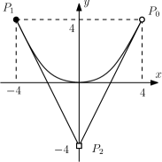
Figure 1. The set $\Delta_{B_{2}}$.

There are three corner points of $\Delta_{B_{2}}$, namely $P_{0}=(4,4),P_{1}=(-4,4)$ and $P_{2}=(0,-4)$. The set $\Delta_{B_{2}}$ is bounded by the lines $y+4\pm 2x=0$ and the parabola $4y=x^{2}$. We want to find a fundamental region in $\sigma\tau$-plane whose elements are in one-to-one correspondence with the elements of $\Delta_{B_{2}}$ under $\varPhi_{B_{2}}$. If $(\sigma,\tau)\equiv(\sigma^{\prime},\tau^{\prime})\pmod{\mathbf{Z}^{2}}$, then it is easy to see that $\varPhi_{B_{2}}(\sigma,\tau)=\varPhi_{B_{2}}(\sigma^{\prime},\tau^{\prime})$. Thus it is enough to consider $0\leq\sigma,\tau\leq 1$. Moreover there are extra symmetries coming from the action of the Weyl group. Observe that $\varPhi_{B_{2}}(\sigma,\tau)$ is equal to any one of the following eight expressions:

$$\begin{array}[]{ll|ll}\text{I}&\varPhi_{B_{2}}(\sigma,\tau)&\text{V}&\varPhi_{B_{2}}(\tau,\sigma)\\ \text{II}&\varPhi_{B_{2}}(-\sigma,\tau)&\text{VI}&\varPhi_{B_{2}}(-\tau,\sigma)\\ \text{III}&\varPhi_{B_{2}}(\sigma,-\tau)&\text{VII}&\varPhi_{B_{2}}(\tau,-\sigma)\\ \text{IV}&\varPhi_{B_{2}}(-\sigma,-\tau)&\text{VIII}&\varPhi_{B_{2}}(-\tau,-\sigma)\end{array}$$

Under these symmetries, the square $0\leq\sigma,\tau\leq 1$ can be separated into eight subtriangles. This is shown in Fig. 2. Define

$$R_{B_{2}}=\{(\sigma,\tau)\in\mathbf{R}^{2}\mathrel{|}0\leq\sigma\leq 1/2\text{ and }\sigma\leq\tau\leq 1/2\}.$$

Note that the restricted function $\varPhi_{B_{2}}:R_{B_{2}}\rightarrow\Delta_{B_{2}}$ is one-to-one and onto. Set $\tilde{P}_{0}=(0,0),\tilde{P}_{1}=(1/2,1/2)$ and $\tilde{P}_{2}=(0,1/2)$. Then $\varPhi_{B_{2}}(\tilde{P}_{i})=P_{i}$ for each $i\in\{1,2,3\}$. This correspondence (and more) is symbolized by the use of different marks, such as circles, disks and squares.

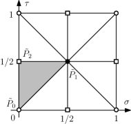
Figure 2. The fundamental region $R_{B_{2}}$.

Now, we are ready analyze the set of fixed points under the bivariate map $\mathcal{B}_{k}$.

Theorem 2.2.

Let $k\geq 2$ be a fixed integer. Then

$$\textnormal{Fix}(\mathcal{B}_{k})=\left\{\varPhi_{B_{2}}\left(\frac{d}{k\pm 1},\frac{e}{k\pm 1}\right):d,e\in\mathbf{Z}\right\}\cup\left\{\varPhi_{B_{2}}\left(\frac{d}{k^{2}\pm 1},\frac{\pm kd}{k^{2}\pm 1}\right):d\in\mathbf{Z}\right\}$$

where the signs of $k^{2}\pm 1$ terms agree.

Proof.

Let $\alpha=\varPhi_{B_{2}}(\sigma,\tau)$ be a fixed point under the map $\mathcal{B}_{k}$. Then we have $\varPhi(k\sigma,k\tau)=\varPhi(\sigma,\tau)$. In the statement of the theorem, there are eight different choices of sign, each one of which corresponds to one of the eight symmetries above. We will prove the theorem for one of these. The others are similar. Suppose that $(k\sigma,k\tau)\equiv(-\tau,\sigma)$ modulo $\mathbf{Z}^{2}$. This is the type VI. In this case

$$k^{2}\sigma\equiv-k\tau\equiv-\sigma\pmod{\mathbf{Z}}.$$

It follows that $\sigma=d/(k^{2}+1)$ and therefore $\tau=-kd/(k^{2}+1)$ for some integer $d$. Thus $\alpha$ is of the form $\varPhi_{B_{2}}(d/(k^{2}+1),-kd/(k^{2}+1))$. ∎

The following theorem gives the cardinality of the set of fixed points under the bivariate map $\mathcal{B}_{k}:\mathbf{C}^{2}\rightarrow\mathbf{C}^{2}$.

Theorem 2.3.

Let $k\geq 2$ be a fixed integer. Then $|\textnormal{Fix}(\mathcal{B}_{k})|=k^{2}$.

Proof.

We follow the idea of Uchimura [Uc09]. The fundamental region $R_{B_{2}}$ is a closed bounded domain. Divide $R_{B_{2}}$ into $k^{2}$ subtriangles $T_{1},\ldots,T_{k^{2}}$ such that each one of them is mapped onto $R_{B_{2}}$ under the multiplication by $k$. This is illustrated for $k=2$ and $k=3$ in Fig. 3.

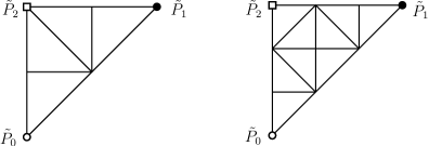
Figure 3. The subtriangles $T_{j}$ of $R_{B_{2}}$ for $k=2$ and $k=3$.

Consider the inverse map from $T_{j}$ to $R_{B_{2}}$ which is division by $k$ together with a suitable linear translation. Being a continuous map there exists at least one fixed point of this map. Moreover there is at most one such point in each $T_{j}$ because of the linearity.

It remains to see that these points are distinct from each other. Such a repetition can occur only at the boundaries of the subtriangles $T_{j}$. However the multiplication by $k$ maps such a boundary to the boundary of $R_{B_{2}}$. The triangles meet at $k$ division points and they are mapped to one of the corner points. On the other hand a corner point $\tilde{P}_{i}$, that is fixed under multiplication by $k$, lies in only one of the triangles $T_{j}$. To see this, observe that $P_{2}$ is fixed under $\mathcal{B}_{k}$ if and only if $k$ is odd. In that case $\tilde{P}_{2}$ is contained in only one of the subtriangles $T_{j}$. ∎

Now, we collect several results we have proved so far and give the following correspondence between $\textnormal{Fix}(\mathcal{B}_{q})$ and $\mathbf{F}_{q}^{2}$.

Lemma 2.4.

Let $q$ be a power a prime $p$ and let $k\geq 2$ be a fixed integer. Consider the cyclotomic number field $K=\mathbf{Q}(\zeta_{q^{4}-1})$ which contain the coordinates of the points fixed under $\mathcal{B}_{k}$. Let $\mathfrak{p}$ be a prime ideal of $K$ lying over $p$. Then there exists a one-to-one correspondence

$$\textnormal{Fix}(\mathcal{B}_{q})\longleftrightarrow\mathbf{F}_{q}^{2}$$

which is given by the reduction modulo $\mathfrak{p}$.

Proof.

There are $q^{2}$ fixed points of $\mathcal{B}_{q}$. We have $\mathcal{B}_{q}\equiv(x^{q},y^{q})\pmod{p}$ by Lemma 2.1. The reduction of each point $(x,y)\in\textnormal{Fix}(\mathcal{B}_{q})$ modulo $\mathfrak{p}$ gives a different solution of the equations $x^{q}-x\equiv 0\pmod{p}$ and $y^{q}-y\equiv 0\pmod{p}$. ∎

This correspondence is compatible with the action of $\mathcal{B}_{k}$. If $\alpha=\varPhi_{B_{2}}(\sigma,\tau)$ is fixed under $\mathcal{B}_{q}$, then its coordinates are algebraic integers. Note that $\mathcal{B}_{k}(\alpha)$ is fixed under $\mathcal{B}_{q}$ too. Let $x\mapsto\overline{x}$ be the reduction map of the theorem. Then we have

$$\overline{\mathcal{B}_{k}(\alpha)}=\mathcal{B}_{k}(\overline{\alpha}).$$

This characterization of $\mathbf{F}_{q}^{2}$, which is compatible with the action of $\mathcal{B}_{k}$, allows us to obtain the main result of this section.

Theorem 2.5.

The bivariate polynomial mapping $\mathcal{B}_{k}$ associated with $B_{2}\cong C_{2}$ induces a permutation of $\mathbf{F}_{q}^{2}$ if and only if $\gcd(q^{4}-1,k)=1$.

Proof.

The theorem is easily verified for $k=0$ and $k=1$. Suppose that $k\geq 2$ and $\gcd(q^{4}-1,k)=1$. In order to see that $\bar{\mathcal{B}}_{k}(x,y)$ is a permutation of $\mathbf{F}_{q}^{2}$, it is enough to see that $\mathcal{B}_{k}$ permute $\textnormal{Fix}(\mathcal{B}_{q})$. By Theorem 2.2, the set $\textnormal{Fix}(\mathcal{B}_{q})$ is explicit. Its elements $\varPhi_{B_{2}}(\sigma,\tau)$ come with rational $\sigma$ and $\tau$ whose denominators are relatively prime to $k$. Thus the map $\mathcal{B}_{k}$ permutes $\textnormal{Fix}(\mathcal{B}_{q})$.

To see the converse, suppose that $\gcd(q^{4}-1,k)\neq 1$. Then there exist an integer $m>1$ dividing either $q^{2}-1$ or $q^{2}+1$. It follows that either $\varPhi_{B_{2}}(1/(q^{2}-1),q/(q^{2}-1))$ or $\varPhi_{B_{2}}(1/(q^{2}+1),q/(q^{2}+1))$ is not in

$$\mathcal{B}_{k}(\textnormal{Fix}(\mathcal{B}_{q}))= \left\{\varPhi_{B_{2}}\left(\frac{kd}{q\pm 1},\frac{ke}{q\pm 1}\right):d,e\in\mathbf{Z}\right\}$$

$$\cup\left\{\varPhi_{B_{2}}\left(\frac{kd}{q^{2}\pm 1},\frac{\pm kqd}{q^{2}\pm 1}\right):d\in\mathbf{Z}\right\}.$$

Thus $\bar{\mathcal{B}}_{k}(x,y)$ is not surjective and as a result it is not a permutation. ∎

Now, we give a counterexample to the conjecture posed by Lidl and Wells in [LW72]. The bivariate map $\bar{\mathcal{B}}_{13}$ is a permutation of $\mathbf{F}_{p}^{2}$ for an infinite number of primes by Theorem 2.5. More precisely $\bar{\mathcal{B}}_{13}:\mathbf{F}_{p}^{2}\rightarrow\mathbf{F}_{p}^{2}$ is a permutation if and only if $p\not\equiv 1,5,8,12\pmod{13}$. Suppose that $\bar{\mathcal{B}}_{13}$ is a composition of linear polynomial vectors and the generalized Chebyshev polynomials $g(2,k,b)$ of Lidl and Wells. Each occurrence of $g(2,k,b)$ will put a restriction on $p$, see Theorem 1.1. However it is not possible to obtain the set of primes $p\not\equiv 1,5,8,12\pmod{13}$ by the conditions $\gcd(k,p^{s}-1)=1$ for $s=1,2,3$. Thus $\bar{\mathcal{B}}_{13}$ cannot be expressed as a composition of linear polynomial vectors and polynomial vectors $g(k,n,b)$ where $k$ and $b$ are various integers.

3. The family associated with $G_{2}$

We refer to [CSM95] for a nice introduction to the theory of Lie algebras. Let $\{\alpha_{1},\alpha_{2}\}$ be a choice of simple roots for the Lie algebra $G_{2}$ with Cartan matrix

$$\left[\begin{array}[]{cc}2&-1\\ -3&2\end{array}\right].$$

The transpose of this matrix transforms the fundamental weights into the fundamental roots. We have

$$\alpha_{1} =2\omega_{1}-3\omega_{2},$$

$$\alpha_{2} =-\omega_{1}+2\omega_{2}.$$

The function $\varPhi_{G_{2}}=(\varphi_{1},\varphi_{2})$ of Theorem 0.1 is obtained by the action of the Weyl group on the fundamental weights $\omega_{1}$ and $\omega_{2}$. The functions $\varphi_{1}$ and $\varphi_{2}$ turn out to be

$$\varphi_{1}(\sigma,\tau)= \ e^{2\pi i\sigma}+e^{2\pi i\tau}+e^{2\pi i(\sigma+\tau)}+e^{-2\pi i\sigma}+e^{-2\pi i\tau}+e^{-2\pi i(\sigma+\tau)},$$

$$\varphi_{2}(\sigma,\tau)= \ e^{2\pi i(2\sigma+\tau)}+e^{2\pi i(\sigma+2\tau)}+e^{2\pi i(\sigma-\tau)}$$

$$\ +e^{-2\pi i(2\sigma+\tau)}+e^{-2\pi i(\sigma+2\tau)}+e^{-2\pi i(\sigma-\tau)}.$$

For each $(\sigma,\tau)\in\mathbf{R}^{2}$, we can simply write

$$\Phi_{G_{2}}(\sigma,\tau)=\ (2\cos(2\pi\sigma)+2\cos(2\pi\tau)+2\cos(2\pi(\sigma+\tau)),$$

$$2\cos(2\pi(2\sigma+\tau)+2\cos(2\pi(\sigma+2\tau))+2\cos(2\pi(\sigma-\tau))).$$

Hofmann and Withers call this map the generalized cosine function for the underlying Lie algebra [HW88]. Theorem 0.1 implies that there are bivariate polynomial mappings $P_{G_{2}}^{k}$, determined from the conditions $\varPhi_{G_{2}}(k\mathbf{x})=P_{G_{2}}^{k}(\varPhi_{G_{2}}(\mathbf{x}))$ where $\mathbf{x}=(\sigma,\tau)$. For simplicity, let us put

$$\mathcal{G}_{k}:=P_{G_{2}}^{k}.$$

These maps satisfy the composition property $\mathcal{G}_{kl}=\mathcal{G}_{k}\circ\mathcal{G}_{l}=\mathcal{G}_{l}\circ\mathcal{G}_{k}$ by their definition. The first few examples of these polynomials are:

$$\mathcal{G}_{0}(x,y)= \ (6,6),$$

$$\mathcal{G}_{1}(x,y)= \ (x,y),$$

$$\mathcal{G}_{2}(x,y)= \ (x^{2}-2x+(-2y-6),-2x^{3}+(6y+18)x+(y^{2}+10y+18)),$$

$$\mathcal{G}_{3}(x,y)= \ (x^{3}+(-3y-9)x+(-6y-12),(-3y-6)x^{3}$$

$$+(9y^{2}+45y+54)x+(y^{3}+18y^{2}+63y+60)),$$

$$\mathcal{G}_{4}(x,y)= \ (x^{4}+(-4y-10)x^{2}+(-4y-8)x+(2y^{2}+8y+6),$$

$$\ 2x^{6}+(-12y-36)x^{4}+(-4y^{2}-28y-40)x^{3}$$

$$+(18y^{2}+108y+162)x^{2}+(12y^{3}+120y^{2}+372y+360)x$$

$$+(y^{4}+24y^{3}+134y^{2}+280y+198)),$$

$$\mathcal{G}_{5}(x,y)= \ (x^{5}+(-5y-15)x^{3}+(-5y-10)x^{2}+(5y^{2}+35y+55)x$$

$$+(10y^{2}+50y+60),(5y+10)x^{6}+(-30y^{2}-150y-180)x^{4}$$

$$+(-5y^{3}-65y^{2}-205y-190)x^{3}+(45y^{3}+360y^{2}+945y+810)x^{2}$$

$$+(15y^{4}+240y^{3}+1200y^{2}+2415y+1710)x$$

$$+(y^{5}+30y^{4}+255y^{3}+920y^{2}+1495y+900)).$$

There is a recurrence relation satisfied by these maps from which it is straightforward to calculate further $\mathcal{G}_{k}$ [Wi88]. If $\mathcal{G}_{k}=(f_{k},g_{k})$, then

$$f_{k+6}= \ x(f_{k+5}+f_{k+1})-(x+y+3)(f_{k+4}+f_{k+2})$$

$$+(x^{2}-2y-4)f_{k+3}-f_{k},$$

$$g_{k+6}= \ y(g_{k+5}+g_{k+1})-(x^{3}-3xy-9x-5y-9)(g_{k+4}+g_{k+2})$$

$$+(y^{2}-2x^{3}+6xy+18x+12y+8)g_{k+3}-g_{k}.$$

Let $q$ be a power of a prime $p$. Note that $\mathcal{G}_{q}\equiv(x^{q},y^{q})\pmod{p}$ for $q=2,3,4$ and $5$. We will show that this is true in general.

Let $\phi(t_{1},t_{2},t_{3})=(t_{1}+1/t_{1},t_{2}+1/t_{2},t_{3}+1/t_{3})$ and $\psi=(\sigma_{1},\sigma_{2},\sigma_{3})$ where $\sigma_{i}$ is the $i$th elementary symmetric function. There exists $G_{k}(x,y,z)$ so that the following diagram commutes:

Commutativity of the upper part follows from the definition of Dickson polynomials. The existence of $G_{k}$ and the fact that each component of $G_{k}$ is in $\mathbf{Z}[x,y,z]$ follows from the fundamental theorem on symmetric polynomials.

Lemma 3.1.

If $t_{1}t_{2}t_{3}=1$ and $\psi(\phi(t_{1},t_{2},t_{3}))=(x,y,z)$, then $z=x^{2}-2y-4$.

Proof.

The proof is by direct computation. Put $t_{3}=1/(t_{1}t_{2})$. We have

$$x =\frac{(t_{2}^{2}+t_{2})t_{1}^{2}+(t_{2}^{2}+1)t_{1}+t_{2}+1}{t_{1}t_{2}}$$

$$y =\frac{t_{2}^{3}t_{1}^{4}+(t_{2}^{4}+t_{2}^{3}+t_{2}^{2}+t_{2})t_{1}^{3}+(t_{2}^{3}+t_{2})t_{1}^{2}+(t_{2}^{3}+t_{2}^{2}+t_{2}+1)t_{1}+t_{2}}{t_{2}^{2}t_{1}^{2}}$$

$$z =\frac{(t_{2}^{4}+t_{2}^{2})t_{1}^{4}+(t_{2}^{4}+2t_{2}^{2}+1)t_{1}^{2}+t_{2}^{2}+1}{t_{2}^{2}t_{1}^{2}}.$$

One can verify that $z=x^{2}-2y-4$. ∎

Define $V=\{(x,y,z)\in\mathbf{C}^{3}:z=x^{2}-2y-4\}$. The map $G_{k}$ induces a map on $V$ because $t_{1}t_{2}t_{3}=1$ implies that $t_{1}^{k}t_{2}^{k}t_{3}^{k}=1$. Let $\pi:V\rightarrow\mathbf{C}^{2}$ be the projection to the first two components, i.e. $\pi(x_{1},x_{2},x_{3})=(x_{1},x_{2})$. We define the bivariate map $\tilde{\mathcal{G}}_{k}$ by the following commutative diagram.

A formula for $\tilde{\mathcal{G}}_{k}(x,y)$ is obtained by replacing $z$ with $x^{2}-2y-4$ in the first two components of $G_{k}$. More precisely $\tilde{\mathcal{G}}_{k}(x,y)=\pi(G_{k}(x,y,x^{2}-2y-4))$. For example

$$\tilde{\mathcal{G}}_{k}(x,y)=(x^{2}+(-2y-6),-2x^{3}-4x^{2}+(4y+8)x+(y^{2}+8y+12)).$$

The bivariate maps $\tilde{\mathcal{G}}_{k}$ and $\mathcal{G}_{k}$ are conjugates to each other. To see this relation, let us consider

$$a =e^{2\pi i\sigma}+e^{-2\pi i\sigma},$$

$$b =e^{2\pi i\tau}+e^{-2\pi i\tau},$$

$$c =e^{2\pi i(\sigma+\tau)}+e^{-2\pi i(\sigma+\tau)}.$$

Then $\varphi_{1}=a+b+c$ and $\varphi_{2}=ab+ac+bc-a-b-c$. In other words $\varphi_{1}=\sigma_{1}$ and $\varphi_{2}=\sigma_{2}-\sigma_{1}$. Let $L:(x,y)\mapsto(x,y-x)$. We have

$$\tilde{\mathcal{G}}_{k}=L\circ\mathcal{G}_{k}\circ L^{-1}.$$

Thus $\tilde{\mathcal{G}}_{k}$ and $\mathcal{G}_{k}$ are conjugate to each other by the linear map $L$. Now, we prove a lemma that is key to obtain the correspondence between $\textnormal{Fix}(\mathcal{G}_{q})$ and $\mathbf{F}_{q}^{2}$.

Lemma 3.2.

Let $q$ be a power of a prime $p$. Then

1. $\tilde{\mathcal{G}}_{q}(x,y)=(x^{q},y^{q})\pmod{p}$,

2. $\mathcal{G}_{q}(x,y)=(x^{q},y^{q})\pmod{p}$.

Proof.

It is enough to prove the first assertion because if that is the case then we have

$$\mathcal{G}_{q}(x,y) \equiv(L^{-1}\circ\tilde{\mathcal{G}}_{k}\circ L)(x,y)\pmod{p}$$

$$\equiv L^{-1}(x^{q},(y-x)^{q})\pmod{p}$$

$$\equiv(x^{q},y^{q})\pmod{p}.$$

By the fundamental theorem on symmetric polynomials, there exists a function $F_{k}\in\mathbf{Z}[x,y,z]$ such that the following diagram commutes:

For example $F_{2}(x,y,z)=(x^{2}-2y,y^{2}-2xz,z^{2})$. Recall that $D_{q}(x)=x^{q}\pmod{p}$. It follows that $G_{q}(x,y,z)=F_{q}(x,y,z)\pmod{p}$. Let $\pi_{1}$ and $\pi_{2}$ be the projections to the first and second components, respectively. Lidl and Wells provide explicit formulas for $\pi_{1}(F_{k})$ and $\pi_{2}(F_{k})$. More precisely

$$\pi_{1}(F_{k}) =\sum_{i=0}^{\lfloor k/2\rfloor}\sum_{j=0}^{\lfloor k/3\rfloor}\frac{k(-1)^{i}}{k-i-2j}\binom{k-i-2j}{i+j}\binom{i+j}{i}x^{k-2i-3j}y^{i}z^{j}$$

$$\pi_{2}(F_{k}) =\sum_{i=0}^{\lfloor k/2\rfloor}\sum_{j=0}^{\lfloor k/3\rfloor}\frac{k(-1)^{j}}{k-i-2j}\binom{k-i-2j}{i+j}\binom{i+j}{i}x^{i}y^{k-2i-3j}z^{i+2j}$$

where only those terms occur for which $k\geq 2i+3j$ [LW72]. It easily follows from these formulas that $\pi(F_{q}(x,y,x^{2}-2y-4))=(x^{q},y^{q})\pmod{p}$. Therefore $\tilde{\mathcal{G}}_{q}(x,y)=\pi(G_{k}(x,y,x^{2}-2y-4))=(x^{q},y^{q})\pmod{p}$. ∎

Let $k\geq 2$ be an integer. Similar to the set $\Delta_{B_{2}}$, the set of points with bounded orbits under $\mathcal{G}_{k}$ is the set

$$\Delta_{G_{2}}=\{\varPhi_{G_{2}}(\sigma,\tau):\sigma,\tau\in\mathbf{R}\}.$$

As a result, a point that is fixed under $\mathcal{G}_{k}:\mathbf{C}^{2}\rightarrow\mathbf{C}^{2}$ is of the form $\varPhi_{G_{2}}(\sigma,\tau)$ for some $\sigma,\tau\in\mathbf{R}$. The set $\Delta_{G_{2}}$, which is shown in Fig. 4, is contained in $\mathbf{R}^{2}$. There are three corner points, namely $Q_{0}=(6,6),Q_{1}=(-3,6)$ and $Q_{2}=(-2,-2)$. The region $\Delta_{G_{2}}$ is enclosed by the singular cubic curve $(y+6x+12)^{2}=4(x+3)^{3}$ and the parabola $4y=x^{2}-12$. The node of the singular cubic curve is at $Q_{1}$.

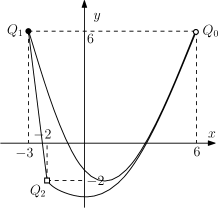
Figure 4. The set $\Delta_{G_{2}}$.

We want to find a fundamental region in $\sigma\tau$-plane whose elements are in one-to-one correspondence with the elements of $\Delta_{G_{2}}$ under $\varPhi_{G_{2}}$. If $(\sigma,\tau)\equiv(\sigma^{\prime},\tau^{\prime})\pmod{\mathbf{Z}^{2}}$, then it is easy to see that $\varPhi_{G_{2}}(\sigma,\tau)=\varPhi_{G_{2}}(\sigma^{\prime},\tau^{\prime})$. Thus it is enough to consider $0\leq\sigma,\tau\leq 1$ to obtain any point in $\Delta_{G_{2}}$ under the map $\varPhi_{G_{2}}$. Moreover there are extra symmetries coming from the action of the Weyl group. Observe that $\varPhi_{G_{2}}(\sigma,\tau)$ is equal to any one of the following twelve expressions:

$$\begin{array}[]{ll|ll|ll}\text{I}&\varPhi_{G_{2}}(\sigma,\tau)&\text{V}&\varPhi_{G_{2}}(\sigma,-\sigma-\tau)&\text{IX}&\varPhi_{G_{2}}(\tau,-\sigma-\tau)\\ \text{II}&\varPhi_{G_{2}}(\tau,\sigma)&\text{VI}&\varPhi_{G_{2}}(-\sigma-\tau,\sigma)&\text{X}&\varPhi_{G_{2}}(-\sigma-\tau,\tau)\\ \text{III}&\varPhi_{G_{2}}(-\sigma,-\tau)&\text{VII}&\varPhi_{G_{2}}(-\sigma,\sigma+\tau)&\text{XI}&\varPhi_{G_{2}}(-\tau,\sigma+\tau)\\ \text{IV}&\varPhi_{G_{2}}(-\tau,-\sigma)&\text{VIII}&\varPhi_{G_{2}}(\sigma+\tau,-\sigma)&\text{XII}&\varPhi_{G_{2}}(\sigma+\tau,-\tau)\end{array}$$

Under these symmetries, the square $0\leq\sigma,\tau\leq 1$ can be separated into twelve subtriangles. This is shown in Fig. 5. Define

$$R_{G_{2}}=\{(\sigma,\tau)\in\mathbf{R}^{2}\mathrel{|}0\leq\sigma\leq 1/3\text{ and }\sigma\leq\tau\leq(1-\sigma)/2\}.$$

Note that the restricted function $\varPhi_{G_{2}}:R_{G_{2}}\rightarrow\Delta_{G_{2}}$ is one-to-one and onto. Set $\tilde{Q}_{0}=(0,0),\tilde{Q}_{1}=(1/3,1/3)$ and $\tilde{Q}_{2}=(0,1/2)$. Then $\varPhi_{G_{2}}(\tilde{Q}_{i})=Q_{i}$ for each $i\in\{1,2,3\}$. This correspondence (and more) is symbolized by the use of different marks, such as circles, disks and square.

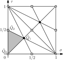
Figure 5. The fundamental region $R_{G_{2}}$.

Now, we are ready analyze the set of fixed points under the bivariate map $\mathcal{G}_{k}$. Let $k\geq 2$ be a fixed integer. Let $\alpha=\varPhi_{G_{2}}(\sigma,\tau)$ be a fixed point under $\mathcal{G}_{k}$. We want to determine the values of $\sigma$ and $\tau$ such that $\mathcal{G}_{k}(\varPhi_{G_{2}}(\sigma,\tau))=\varPhi_{G_{2}}(k\sigma,k\tau)=\varPhi_{G_{2}}(\sigma,\tau)$. There are twelve possibilities. For example, let us consider $(k\sigma,k\tau)\equiv(-\sigma-\tau,\sigma)$ modulo $\mathbf{Z}^{2}$. This is the case VI. We have

$$k^{2}\sigma\equiv-k\sigma-k\tau\equiv-k\sigma-\sigma\pmod{\mathbf{Z}}.$$

It follows that $\sigma=d/(k^{2}+k+1)$ for some integer $d$. Since $k\sigma\equiv-\sigma-\tau\pmod{\mathbf{Z}}$, we have $\tau\equiv-(k+1)\sigma\pmod{\mathbf{Z}}$. Thus

$$\alpha=\varPhi_{G_{2}}\left(\frac{d}{k^{2}+k+1},\frac{-(k+1)d}{k^{2}+k+1}\right)=\varPhi_{G_{2}}\left(\frac{d}{k^{2}+k+1},\frac{kd}{k^{2}+k+1}\right).$$

Here, the second equality follows from $d+kd-(k+1)d\equiv 0\pmod{k^{2}+k+1}$ and the definition of $\varPhi_{G_{2}}$. In general, a fixed point $\alpha$ fits into one of the following sets:

$$S_{1} =\left\{\varPhi_{G_{2}}\left(\frac{d}{k-1},\frac{e}{k-1}\right):d,e\in\mathbf{Z}\right\},$$

$$S_{2} =\left\{\varPhi_{G_{2}}\left(\frac{d}{k^{2}-1},\frac{dk}{k^{2}-1}\right):d\in\mathbf{Z}\right\},$$

$$S_{3} =\left\{\varPhi_{G_{2}}\left(\frac{d}{k^{2}+k+1},\frac{dk}{k^{2}+k+1}\right):d\in\mathbf{Z}\right\},$$

$$S_{4} =\left\{\varPhi_{G_{2}}\left(\frac{d}{k+1},\frac{e}{k+1}\right):d,e\in\mathbf{Z}\right\},$$

$$S_{5} =\left\{\varPhi_{G_{2}}\left(\frac{d}{k^{2}-1},\frac{d(-k)}{k^{2}-1}\right):d\in\mathbf{Z}\right\},$$

$$S_{6} =\left\{\varPhi_{G_{2}}\left(\frac{d}{k^{2}-k+1},\frac{d(-k)}{k^{2}-k+1}\right):d\in\mathbf{Z}\right\}.$$

The computation above shows that the fixed points of type VI takes place in $S_{3}$. One can do similar computations for the other cases and obtain the following table which gives the correspondence between the sets $S_{i}$ and the types of symmetries.

$$\begin{array}[]{|c|c|c|c|c|c|}\hline\cr S_{1}&S_{2}&S_{3}&S_{4}&S_{5}&S_{6}\\ \hline\cr\text{I}&\text{II, V}&\text{VI, IX, X }&\text{III }&\text{IV, VII}&\text{VIII,XI,XII}\\ \hline\cr\end{array}$$

Theorem 3.3.

Let $k\geq 2$ be a fixed integer. Then

$$\textnormal{Fix}(\mathcal{G}_{k})=S_{1}\cup S_{2}\cup S_{3}\cup S_{4}\cup S_{5}\cup S_{6}.$$

Note that the union $\cup S_{i}$ is not disjoint. For example the point $Q_{0}$ is contained in each $S_{i}$. The following theorem gives the cardinality of the set of points fixed under $\mathcal{G}_{k}$.

Theorem 3.4.

Let $k\geq 2$ be a fixed integer. Then $|\textnormal{Fix}(\mathcal{G}_{k})|=k^{2}$.

Proof.

We follow the idea of Uchimura [Uc09]. The fundamental region $R_{G_{2}}$ is a closed bounded domain. Divide $R_{G_{2}}$ into $k^{2}$ subtriangles $T_{1},\ldots,T_{k^{2}}$ such that each one of them is mapped onto $R_{G_{2}}$ under the multiplication by $k$. This is illustrated for $k=2$ and $k=3$ in Figure 6.

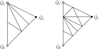
Figure 6. The subtriangles $T_{j}$ of $R_{G_{2}}$ for $k=2$ and $k=3$.

Note that $Q_{1}$ is fixed under $\mathcal{G}_{k}$ if and only if $k$ is not divisible by $3$. In that case $\tilde{Q}_{1}$ is contained in only one of the subtriangles $T_{j}$. Similarly $Q_{2}$ is fixed under $\mathcal{G}_{k}$ if and only if $k$ is odd. In such a case, the point $\tilde{Q}_{2}$ is contained in only one of the subtriangles $T_{j}$ as well. The rest of the proof is as the same as the proof of Theorem 2.3. ∎

The proof of the following lemma is similar to the proof of Lemma 2.4 and omitted.

Lemma 3.5.

Let $q$ be a power a prime $p$ and let $k\geq 2$ be a fixed integer. Consider the cyclotomic number field $K=\mathbf{Q}(\zeta_{q^{6}-1})$ which contain the coordinates of the points fixed under $\mathcal{G}_{k}$. Let $\mathfrak{p}$ be a prime ideal of $K$ lying over $p$. Then there exists a one-to-one correspondence

$$\textnormal{Fix}(\mathcal{G}_{q})\longleftrightarrow\mathbf{F}_{q}^{2}$$

which is given by the reduction modulo $\mathfrak{p}$.

Similar to the case associated with $B_{2}\cong C_{2}$, the correspondence given by this lemma is compatible with the action of $\mathcal{G}_{k}$. If $\alpha=\varPhi_{G_{2}}(\sigma,\tau)$ is fixed under $\mathcal{G}_{q}$, then $\mathcal{G}_{k}(\alpha)$ is fixed under $\mathcal{G}_{q}$ too. Moreover

$$\overline{\mathcal{G}_{k}(\alpha)}=\mathcal{G}_{k}(\overline{\alpha}).$$

The characterization of $\mathbf{F}_{q}^{2}$, which is compatible with the action of $\mathcal{G}_{k}$, allows us to obtain the main result of this section.

Theorem 3.6.

The bivariate polynomial mapping $\mathcal{G}_{k}$ associated with $G_{2}$ induces a permutation of $\mathbf{F}_{q}^{2}$ if and only if $\gcd(k,q^{6}-1)=1$.

Proof.

The theorem is easily verified for $k=0$ and $k=1$. Suppose that $k\geq 2$ and $\gcd(k,q^{6}-1)=1$. In order to see that $\bar{\mathcal{G}}_{k}(x,y)$ is a permutation of $\mathbf{F}_{q}^{2}$, it is enough to see that $\mathcal{G}_{k}$ permute $\textnormal{Fix}(\mathcal{G}_{q})$. By Theorem 3.3, the set $\textnormal{Fix}(\mathcal{G}_{q})$ is explicit. Its elements $\varPhi_{G_{2}}(\sigma,\tau)$ come with rational $\sigma$ and $\tau$ whose denominators are relatively prime to $k$. Thus the map $\mathcal{G}_{k}$ permutes $\textnormal{Fix}(\mathcal{G}_{q})$.

To see the converse, suppose that $\gcd(k,q^{6}-1)\neq 1$. Let $n$ be an integer such that $n\in\{q^{2}-1,q^{2}+1,q^{2}-q+1,q^{2}+q+1\}$ and $\gcd(k,n)>1$. Consider the element

$$\alpha=\varPhi_{G_{2}}\left(\frac{1}{n},\frac{\pm q}{n}\right)$$

with a suitable choice of sign so that $\alpha\in\textnormal{Fix}(\mathcal{G}_{q})$. The element $\alpha$ is in $\textnormal{Fix}(\mathcal{G}_{q})$ but it is not in $\mathcal{G}_{k}(\textnormal{Fix}(\mathcal{G}_{q}))$. As a result, the map $\mathcal{G}_{k}$, restricted to $\textnormal{Fix}(\mathcal{G}_{q})$, is not surjective. Thus $\bar{\mathcal{G}}_{k}(x,y)$ is not a permutation. ∎

Now, we give a counterexample to the conjecture posed by Lidl and Wells in [LW72]. The bivariate map $\bar{\mathcal{G}}_{13}$ is a permutation of $\mathbf{F}_{p}^{2}$ for an infinite number of primes by Theorem 3.6. More precisely $\bar{\mathcal{G}}_{13}:\mathbf{F}_{p}^{2}\rightarrow\mathbf{F}_{p}^{2}$ is a permutation if and only if $p\not\equiv 1,3,4,9,10,12\pmod{13}$. Suppose that $\bar{\mathcal{G}}_{13}$ is a composition of linear polynomial vectors and the generalized Chebyshev polynomials $g(2,k,b)$ of Lidl and Wells. Each occurrence of $g(2,k,b)$ will put a restriction on $p$, see Theorem 1.1. However it is not possible to obtain the set of primes $p\not\equiv 1,3,4,9,10,12\pmod{13}$ by the conditions $\gcd(k,p^{s}-1)=1$ for $s=1,2,3$. Thus $\bar{\mathcal{G}}_{13}$ cannot be expressed as a composition of linear polynomial vectors and polynomial vectors $g(k,n,b)$ where $k$ and $b$ are various integers.

References

[CSM95]
R. Carter, G. Segal, I. Macdonald, Lectures on Lie groups and Lie
algebras. London Mathematical Society Student Texts, 32.
Cambridge University Press, Cambridge, 1995.
[Fa24]
P. Fatou, Sur l’itération analytique et les substitutions permutables,
J. Math. Pure. Appl. 23 (1924), 1–49.
[Fr70] M. Fried, On a conjecture of Schur. Michigan
Math. J. (1970), 17, 41–55.
[HW88]
M. E. Hoffman and W. D. Withers; Generalized Chebyshev polynomials
associated with affine Weyl groups. Trans. Amer. Math. Soc. 308 (1988),
91–104.
[Ju22]
G. Julia, Mémoire sur la permutabilité des fractions
rationnelles.
Ann. Sci. École Norm. Sup. (3) 39 (1922), 131–215.
[Kü14]
Ö. Küçüksakallı, Value sets of Lattès maps over finite
fields. J. Number Theory 143 (2014), 262–278.
[LN83]
R. Lidl, H. Niederreiter, Finite fields, Encyclopedia of Mathematics and
its Applications, Vol. 20. Cambridge, UK: Cambridge University Press, 1983.
[LW72]
R. Lidl, C. Wells, Chebyshev polynomials in several variables.
J. Reine Angew. Math. 255 (1972), 104–111.
[Mü97]
P. Müller, A Weil-bound free proof of Schur’s conjecture.
Finite Fields Appl. 3 (1997), no. 1, 25–32.
[Ri23]
J. F. Ritt, Permutable rational functions.
Trans. Amer. Math. Soc. 25 (1923), no. 3, 399–448.
[Si07]
J. H. Silverman, The arithmetic of dynamical systems.
Graduate Texts in Mathematics, 241. Springer, New York, 2007.
[Tu95]
G. Turnwald, On Schur’s conjecture. J. Austral. Math. Soc. Ser. A 58
(1995), no. 3, 312–357.
[Uc09]
K. Uchimura, Generalized Chebyshev maps of and their
perturbations. Osaka J. Math. 46 (2009), no. 4, 995–1017.
[Ve87]
A. P. Veselov, Integrable mappings and Lie algebras. Soviet Math.
Dokl. 35 (1987), 211–213.
[Ve91]
A. P. Veselov, Integrable mappings. Russian Math. Surveys 46 (1991),
no. 5, 1–51.
[Wi88]
W. D. Withers, Folding polynomials and their dynamics.
Amer. Math. Monthly 95 (1988), no. 5, 399–413.