Novel solvable many-body problems

Abstract

Novel classes of dynamical systems are introduced, including many-body problems characterized by nonlinear equations of motion of Newtonian type (“acceleration equals forces”) which determine the motion of points in the complex plane. These models are solvable, namely their configuration at any time can be obtained from the initial data by algebraic operations, amounting to the determination of the zeros of a known time-dependent polynomial in the independent variable $z$. Some of these models are multiply periodic, isochronous or asymptotically isochronous; others display scattering phenomena.

2000 Mathematics Subject Classification: 12D99, 70F10, 70K42.

1 Introduction

Notation 1.1. Unless otherwise indicated, hereafter $N$ is an arbitrary positive integer, $N\geq 2$, indices such as $n,$ $m,$ $\ell,$ $...$ run over the integers from $1$ to $N$, and superimposed arrows denote $N$-vectors: for instance the vector $\vec{c}$ has the $N$ components $c_{m}$. We use instead a superimposed tilde to denote an unordered set of $N$ numbers: for instance the notation $\tilde{z}$ denotes the unordered set of $N$ numbers $z_{n}$, say, the $N$ zeros of a polynomial of degree $N$ in $z$. Upper-case boldface letters denote $N\times N$ matrices: for instance the matrix $\mathbf{M}$ features the $N^{2}$ elements $M_{nm}$. The numbers we use are generally assumed to be complex; except for those restricted to be positive integers (see above), which generally play the role of indices; and except for the “time”  variable, see below. The imaginary unit is hereafter denoted as $\mathbf{i}$, implying of course $\mathbf{i}^{2}=-1$. For quantities depending on the real independent variable $t$ (“time”), superimposed dots indicate differentiation with respect to it: so, for instance, $\dot{z}_{n}\left(t\right)\equiv dz_{n}\left(t\right)/dt$, $\ddot{z}_{n}\equiv d^{2}z_{n}/dt^{2}$; but often the $t$-dependence is not explicitly indicated, whenever this is unlikely to cause any misunderstanding (as, for instance, in the second formula we just wrote and below in (3)). The Kronecker symbol $\delta_{nm}$ has the usual meaning: $\delta_{nm}=1$ if $n=m$, $\delta_{nm}=0$ if $n\neq m$; and we denote below as $\mathbf{I}$ the unit $N\times N$ matrix the elements of which are $\delta_{nm}$. We adopt throughout the usual convention according to which a void sum vanishes and a void product equals unity: $\sum_{j=J}^{K}f_{j}=0,$ $\prod\nolimits_{j=J}^{K}f_{j}=1$ if $J>K$. Moreover we introduce the following convenient notations:

$$\sigma_{m}\left(\vec{z}\right)=\sum_{1\leq s_{1}<s_{2}<...<s_{m}\leq N}\left(z_{s_{1}}z_{s_{2}}\cdots z_{s_{m}}\right)~{},$$ (1a)

$$\sigma_{n,m}\left(\vec{z}\right)=\delta_{1m}+\sum_{{\footnotesize 1\leq s_{1}<s_{2}<\ldots<s_{m-1}\leq N~{};~{}s_{j}\neq n,~{}j=1,...m-1}}\left(z_{s_{1}}z_{s_{2}}\cdots z_{s_{m-1}}\right)~{},$$ (1b)

$$\sigma_{n_{1}n_{2},m}\left(\vec{z}\right)=\delta_{2m}+\sum_{\begin{subarray}{c}{\footnotesize 1\leq s_{1}<s_{2}<\ldots<s_{m-2}\leq N~{};}\\ {\footnotesize s_{j}\neq n}_{1},~{}{\footnotesize s_{j}\neq n_{2},~{}j=1,...m-2}\end{subarray}}\left(z_{s_{1}}z_{s_{2}}\cdots z_{s_{m-2}}\right)~{},$$ (1c)

$$\sigma_{n_{1}n_{2}n_{3},m}\left(\vec{z}\right)=\delta_{3m}+\sum_{\begin{subarray}{c}{\footnotesize 1\leq s_{1}<s_{2}<\ldots<s_{m-3}\leq N~{};}\\ {\footnotesize s_{j}\neq n}_{1}{\footnotesize,~{}s_{j}\neq n_{2},~{}s_{j}\neq n_{3},~{}j=1,...m-3}\end{subarray}}\left(z_{s_{1}}z_{s_{2}}\cdots z_{s_{m-3}}\right)~{},$$ (1d)

where of course the symbol $$\sum_{1\leq s_{1}<s_{2}<...<s_{m}\leq N} 1 N m s_{1},s_{2},\ldots,s_{m} s_{1}<s_{2}<\ldots<s_{m} \sum_{{\footnotesize 1\leq s_{1}<s_{2}<\ldots<s_{m-1}\leq N~{};~{}s_{j}\neq n,~{}j=1,...m-1}} 1 N m-1 s_{1},s_{2},\ldots,s_{m-1} s_{1}<s_{2}<\ldots<s_{m-1} n; \sum_{{\footnotesize 1\leq s_{1}<s_{2}<\ldots<s_{m-2}\leq N~{};~{}s_{j}\neq n}_{1},~{}{\footnotesize s_{j}\neq n_{2},~{}j=1,...m-2}} \sum_{{\footnotesize 1\leq s_{1}<s_{2}<\ldots<s_{m-3}\leq N~{};~{}s_{j}\neq n}_{1}{\footnotesize,~{}s_{j}\neq n_{2},~{}s_{j}\neq n_{3},~{}j=1,...m-3}} \sigma_{n,1}(\vec{z})=1, \sigma_{n_{1}n_{2},1}\left(\vec{z}\right)=0 \sigma_{n_{1}n_{2},2}\left(\vec{z}\right)=1, \sigma_{n_{1}n_{2}n_{3},m}\left(\vec{z}\right)=0 m\leq 2 \sigma_{n_{1}n_{2}n_{3},3}\left(\vec{z}\right)=1 n N N\leq 3 1 N k \ell_{1}, \ell_{2}, \ell_{k} N\leq k \blacksquare$$ denotes the sum from to over the integer indices with the restriction that , while the symbol denotes the sum from to over the indices with the restriction and moreover the requirement that all these indices be different from and likewise for the symbols and . Note that—according to the convention (see above) that a sum over an empty set of indices equals zero—these definitions imply and and for while . Finally, the prime appended to a sum (see for instance below (3) and also note the simplification it would imply for (1b)) indicates that the sum runs—over the indicated indices, in the identified range—with the additional restrictions that these indices be all different among themselves and moreover all different from the “outside” index (which is for instance in (3)); note that this sum becomes void hence vanishes identically if is small enough, so for instance the last sum in the left-hand side of (3d) vanishes for , and more generally the “primed” sum from to over indices …, vanishes identically if .

Remark 1.1. Note that the notation $\sigma_{m}\left(\tilde{z}\right)$ (instead of $\sigma_{m}\left(\vec{z}\right)$) is equally meaningful, since this quantity, see (1a), only depends on symmetrical sums of the $N$ components $z_{m}$ of the $N$-vector $\vec{z},$ hence it is independent of the ordering of the $N$ elements $z_{n}$ of the unordered set $\tilde{z}$. The notations $\sigma_{n,m}\left(\tilde{z}\right)$, $\sigma_{n_{1}n_{2},m}\left(\tilde{z}\right)$, $\sigma_{n_{1}n_{2}n_{3},m}\left(\tilde{z}\right),$ see (1), are instead ill-defined and cannot therefore be used; except in the context of expressions which remain valid for any ordering of the $N$ numbers $z_{n}$, i. e., for any assignments of the $N$ different integer labels $n$ (in the range $1\leq n\leq N)$ to the $N$ elements of the unordered set $\tilde{z}$; provided of course that assignment is maintained throughout that expression (in which case the relevant expression amounts in fact to $N!$ different formulas; assuming, as we generally do, that the $N$ numbers $z_{n}$ are all different among themselves). This remark is of course equally valid for any function $f\left(\tilde{z}\right)$. $\blacksquare$

The main protagonists of this paper are formulas relating the time-evolution of the $N$ zeros $z_{n}\left(t\right)$ of a time-dependent monic polynomial of degree $N$ in the independent variable $z,$

$$p_{N}\left(z;~{}\vec{c}\left(t\right),~{}\tilde{z}\left(t\right)\right)=\prod\limits_{n=1}^{N}\left[z-z_{n}\left(t\right)\right]~{},$$ (2a)

to the time-evolution of its $$N c_{m}\left(t\right),$$ coefficients

$$p_{N}\left(z;~{}\vec{c}\left(t\right),~{}\tilde{z}\left(t\right)\right)=z^{N}+\sum_{m=1}^{N}\left[c_{m}\left(t\right)~{}z^{N-m}\right]~{}.$$ (2b)

The first two of these formulas read as follows [1]:

$$\dot{z}_{n}=-\left[\prod\limits_{\ell=1,~{}\ell\neq n}^{N}\left(z_{n}-z_{\ell}\right)^{-1}\right]~{}\sum_{m=1}^{N}\left[\dot{c}_{m}~{}\left(z_{n}\right)^{N-m}\right]~{},$$ (3a)

$$\ddot{z}_{n}-\sum_{\ell=1}^{N}{}^{\prime}\left(\frac{2~{}\dot{z}_{n}~{}\dot{z}_{\ell}}{z_{n}-z_{\ell}}\right)=-\left[\prod\limits_{\ell=1,~{}\ell\neq n}^{N}\left(z_{n}-z_{\ell}\right)^{-1}\right]~{}\sum_{m=1}^{N}\left[\ddot{c}_{m}~{}\left(z_{n}\right)^{N-m}\right]~{}.$$ (3b)

In the present paper we report two additional formulas of this kind:

$$\dddot{z}_{n}-3~{}\sum_{\ell=1}^{N}{}^{\prime}\left(\frac{\ddot{z}_{n}~{}\dot{z}_{\ell}+\ddot{z}_{\ell}~{}\dot{z}_{n}}{z_{n}-z_{\ell}}\right)+3~{}\sum_{\ell_{1},\ell_{2}=1}^{N}{}^{\prime}\left[\frac{\dot{z}_{n}~{}\dot{z}_{\ell_{1}}~{}\dot{z}_{\ell_{2}}}{\left(z_{n}-z_{\ell_{1}}\right)~{}\left(z_{n}-z_{\ell_{2}}\right)}\right]$$ (3c)

$$= -\left[\prod\limits_{\ell=1,~{}\ell\neq n}^{N}\left(z_{n}-z_{\ell}\right)^{-1}\right]~{}\sum_{m=1}^{N}\left[\dddot{c}_{m}~{}\left(z_{n}\right)^{N-m}\right]~{},$$

$$\ddddot{z}_{n}-\sum_{\ell=1}^{N}{}^{\prime}\left(\frac{4~{}\dddot{z}_{n}~{}\dot{z}_{\ell}+4~{}\dddot{z}_{\ell}~{}\dot{z}_{n}+6~{}\ddot{z}_{n}~{}\ddot{z}_{\ell}}{z_{n}-z_{\ell}}\right)$$ (3d)

$$+6~{}\sum_{\ell_{1},\ell_{2}=1}^{N}{}^{\prime}\left[\frac{\ddot{z}_{n}~{}\dot{z}_{\ell_{1}}~{}\dot{z}_{\ell_{2}}+2~{}\ddot{z}_{\ell_{1}}~{}\dot{z}_{\ell_{2}}~{}\dot{z}_{n}}{\left(z_{n}-z_{\ell_{1}}\right)~{}\left(z_{n}-z_{\ell_{2}}\right)}\right]$$

$$-4~{}\sum_{\ell_{1},\ell_{2},~{}\ell_{3}=1}^{N}{}^{\prime}\left[\frac{\dot{z}_{n}~{}\dot{z}_{\ell_{1}}~{}\dot{z}_{\ell_{2}}~{}\dot{z}_{\ell_{3}}}{\left(z_{n}-z_{\ell_{1}}\right)~{}\left(z_{n}-z_{\ell_{2}}\right)~{}\left(z_{n}-z_{\ell_{3}}\right)}\right]$$

$$= -\left[\prod\limits_{\ell=1,~{}\ell\neq n}^{N}\left(z_{n}-z_{\ell}\right)^{-1}\right]~{}\sum_{m=1}^{N}\left[\ddddot{c}_{m}~{}\left(z_{n}\right)^{N-m}\right]~{}.$$

A terse outline of the proof of these identities is reported in Appendix A.

The first two of the formulas (3) have recently allowed the identification of (endless sequences of) new solvable many-body problems characterized by nonlinear equations of motion of Newtonian type (“acceleration equals forces”) determining the motion of $N$ points in the complex $z$-plane [1, 2, 3, 4]. In the present paper we show how the last two of the formulas (3) allow the identification of additional endless sequences of new solvable dynamical systems determining the motion of points in the complex $z$-plane—also including many-body problems characterized by nonlinear equations of motion of Newtonian type (“acceleration equals forces”).

Note that the notation (2), which we employ for polynomials, is somewhat redundant, since they are equally well defined by the (time-dependent) $N$-vector $\vec{c}\left(t\right)$ the $N$ components of which are the $N$ coefficients $c_{m}\left(t\right)$ of the polynomial (see (2b)), as by the (time-dependent) unordered set $\tilde{z}\left(t\right)$ the $N$ elements of which are the $N$ zeros $z_{n}\left(t\right)$ of the polynomial (see (2a)). Indeed the $N$ coefficients $c_{m}\left(t\right)$ can be explicitly expressed in terms of the $N$ zeros $z_{n}\left(t\right)$ as follows:

$$c_{m}=\left(-1\right)^{m}~{}\sigma_{m}\left(\vec{z}\right)\equiv\left(-1\right)^{m}~{}\sigma_{m}\left(\tilde{z}\right)$$ (4)

(see Notation 1.1 and Remark 1.1). While the $N$ zeros $z_{n}\left(t\right)$ are likewise uniquely determined (up to permutations) by the $N$ coefficients $c_{m}\left(t\right)$, but of course explicit expressions to this effect are generally available only for $N\leq 4$.

There holds moreover the following identity:

$$\left(z_{n}\right)^{N}+\sum_{m=1}^{N}\left[c_{m}~{}\left(z_{n}\right)^{N-m}\right]=0~{},$$ (5a)

which is an obvious consequence of (2), and via (4) it implies

$$\left(z_{n}\right)^{N}+\sum_{m=1}^{N}\left[\left(-1\right)^{m}~{}\sigma_{m}\left(\tilde{z}\right)~{}\left(z_{n}\right)^{N-m}\right]=0~{}.$$ (5b)

Note that, while the formula (5a) is an identity valid for the $$N c_{m} N z_{n} N z_{n} \tilde{z}$$ coefficients and the zeros of any polynomial, see (2), the identity (5b) is clearly valid for any arbitrary assignment of the elements of the unordered set .

Likewise, there holds the following formula that is also clearly valid for any assignment of the $N$ elements $z_{n}$ of the unordered set $\tilde{z}$ (see Notation 1.1 and Remark 1.1):

$$-\left[\prod\limits_{\ell=1,~{}\ell\neq n}^{N}\left(z_{n}-z_{\ell}\right)^{-1}\right]~{}\sum_{j=1}^{N}\left[\left(-1\right)^{j}~{}\left(z_{n}\right)^{N-j}~{}\sigma_{m,j}\left(\tilde{z}\right)\right]=\delta_{nm}~{};$$ (6a)

and note that this formula can also be rewritten in the following $$\left(N\times N\right)$$-matrix version:

$$\left[\mathbf{R}\left(\tilde{z}\right)\right]_{nm}\equiv R_{nm}\left(\tilde{z}\right)=-\left[\prod\limits_{\ell=1,~{}\ell\neq n}^{N}\left(z_{n}-z_{\ell}\right)^{-1}\right]~{}\left(z_{n}\right)^{N-m}~{},$$ (6b)

$$\left[\mathbf{R}^{-1}\left(\tilde{z}\right)\right]_{nm}\equiv\left[R^{-1}\left(\tilde{z}\right)\right]_{nm}=\left(-1\right)^{n}~{}\sigma_{n,m}\left(\tilde{z}\right)~{},$$ (6c)

implying of course (see Notation 1.1 and Remark 1.1)

$$\mathbf{R}\left(\tilde{z}\right)~{}\mathbf{R}^{-1}\left(\tilde{z}\right)=\mathbf{R}^{-1}\left(\tilde{z}\right)~{}\mathbf{R}\left(\tilde{z}\right)=\mathbf{I~{}.}$$ (6d)

Finally let us report $3$ additional identities which are obvious consequences of the definitions (4) and (1) (see Notation 1.1 and Remark 1.1):

$$\dot{c}_{m}=\left(-1\right)^{m}~{}\dot{\sigma}_{m}\left(\vec{z}\right)\equiv\left(-1\right)^{m}~{}\sum_{n=1}^{N}\left[\sigma_{n,m}\left(\tilde{z}\right)~{}\dot{z}_{n}\right]~{},$$ (7a)

$$\ddot{c}_{m}=\left(-1\right)^{m}~{}\ddot{\sigma}_{m}\left(\vec{z}\right)$$

$$\equiv\left(-1\right)^{m}~{}\left\{\sum_{n=1}^{N}\left[\sigma_{n,m}\left(\tilde{z}\right)~{}\ddot{z}_{n}\right]+\sum_{n_{1},n_{2}=1,n_{1}\neq n_{2}}^{N}\left[\sigma_{n_{1}n_{2},m}\left(\tilde{z}\right)~{}\dot{z}_{n_{1}}~{}\dot{z}_{n_{2}}\right]\right\}~{},$$ (7b)

$$\dddot{c}_{m}=\left(-1\right)^{m}~{}\dddot{\sigma}_{m}\left(\vec{z}\right)\equiv\left(-1\right)^{m}~{}\left\{\sum_{n=1}^{N}\left[\sigma_{n,m}\left(\tilde{z}\right)~{}\dddot{z}_{n}\right]\right.$$

$$\left.+3~{}\sum_{n_{1},n_{2}=1,n_{1}\neq n_{2}}^{N}\left[\sigma_{n_{1}n_{2},m}\left(\tilde{z}\right)~{}\ddot{z}_{n_{1}}~{}\dot{z}_{n_{2}}\right]\right.$$

$$\left.+\sum_{n_{1},n_{2},n_{3}=1,n_{1}\neq n_{2}\neq n_{3}}^{N}\left[\sigma_{n_{1}n_{2}n_{3},m}\left(\tilde{z}\right)~{}\dot{z}_{n_{1}}~{}\dot{z}_{n_{2}}~{}\dot{z}_{n_{3}}\right]\right\}~{},$$ (7c)

where the indices $$n_{1},n_{2},n_{3}$$ in the last sum all different among themselves.

In Section 3 it is indicated how these polynomial properties are instrumental to identify endless classes of solvable dynamical systems including many-body problems of Newtonian type, one of which is immediately reported in the following Section 2, while some of its solutions are displayed in Appendix B. The paper is then concluded by a section entitled “Outlook”, where further investigations are tersely outlined.

2 Display and discussion of a novel solvable many-body problem

In this section we provide and discuss an instance of the novel solvable many-body problems of Newtonian type identified in this paper. Its equations of motion, characterizing the time-evolution of the $2N$ complex dependent variables $z_{n}\equiv z_{n}\left(t\right)$ and $w_{n}\equiv w_{n}\left(t\right),$ read as follows:

$$\ddot{z}_{n}=w_{n}~{},$$ (8a)

$$\ddot{w}_{n}=\sum_{\ell=1}^{N}{}^{\prime}\left(\frac{4~{}\dot{w}_{n}~{}\dot{z}_{\ell}+4~{}\dot{w}_{\ell}~{}\dot{z}_{n}+6~{}w_{n}~{}w_{\ell}}{z_{n}-z_{\ell}}\right)$$

$$-6~{}\sum_{\ell_{1},\ell_{2}=1}^{N}{}^{\prime}\left[\frac{w_{n}~{}\dot{z}_{\ell_{1}}~{}\dot{z}_{\ell_{2}}+2~{}w_{\ell_{1}}~{}\dot{z}_{n}~{}\dot{z}_{\ell_{2}}}{\left(z_{n}-z_{\ell_{1}}\right)~{}\left(z_{n}-z_{\ell_{2}}\right)}\right]$$

$$+4~{}\sum_{\ell_{1},\ell_{2},~{}\ell_{3}=1}^{N}{}^{\prime}\left[\frac{\dot{z}_{n}~{}\dot{z}_{\ell_{1}}~{}\dot{z}_{\ell_{2}}~{}\dot{z}_{\ell_{3}}}{\left(z_{n}-z_{\ell_{1}}\right)~{}\left(z_{n}-z_{\ell_{2}}\right)~{}\left(z_{n}-z_{\ell_{3}}\right)}\right]-\left[\prod\limits_{\ell=1,~{}\ell\neq n}^{N}\left(z_{n}-z_{\ell}\right)^{-1}\right]\cdot$$

$$\cdot\sum_{m=1}^{N}\left[\left(\alpha_{m}~{}\dddot{c}_{m}+\beta_{m}~{}\ddot{c}_{m}+\gamma_{m}~{}\dot{c}_{m}+\delta_{m}~{}c_{m}\right)~{}\left(z_{n}\right)^{N-m}\right]~{},$$ (8b)

with $$c_{m} \dot{c}_{m} z_{n} \dot{z}_{n} \ddot{c}_{m} \dddot{c}_{m} z_{n} w_{n} \dot{z}_{n} \dot{w}_{n}$$, expressed in terms of and by (7a) and (4) and , expressed in terms of the dependent variables , and their time derivatives , as follows (see Notation 1.1 and Remark 1.1),

$$\ddot{c}_{m}=\left(-1\right)^{m}~{}\left\{\sum_{n=1}^{N}\left[\sigma_{n,m}\left(\tilde{z}\right)~{}w_{n}\right]+\sum_{n_{1},n_{2}=1}^{N}\left[\sigma_{n_{1}n_{2},m}\left(\tilde{z}\right)~{}\dot{z}_{n_{1}}~{}\dot{z}_{n_{2}}\right]\right\}~{},$$ (8c)

$$\dddot{c}_{m}=\left(-1\right)^{m}~{}\left\{\sum_{n=1}^{N}\left[\sigma_{n,m}\left(\tilde{z}\right)~{}\dot{w}_{n}\right]+3~{}\sum_{n_{1},n_{2}=1}^{N}\left[\sigma_{n_{1}n_{2},m}\left(\tilde{z}\right)~{}w_{n_{1}}~{}\dot{z}_{n_{2}}\right]\right.$$

$$\left.+\sum_{n_{1},n_{2},n_{3}=1}^{N}\left[\sigma_{n_{1}n_{2}n_{3},m}\left(\tilde{z}\right)~{}\dot{z}_{n_{1}}~{}\dot{z}_{n_{2}}~{}\dot{z}_{n_{3}}\right]\right\}~{}.$$ (8d)

In (8b) the parameters $$\alpha_{m},~{}\beta_{m},~{}\gamma_{m},~{}\delta_{m} 4N 8N a_{m}^{\left(1\right)} a_{m}^{\left(2\right)} a_{m}^{\left(3\right)} a_{m}^{\left(4\right)} \omega_{m}^{\left(1\right)} \omega_{m}^{\left(2\right)} \omega_{m}^{\left(3\right)} \omega_{m}^{\left(4\right)}$$ are arbitrary complex numbers, which may be conveniently related to the real parameters , , , , , , , (for their role see below eq. (10)) by the following formulas

$$\alpha_{m}=-a_{m}^{(1)}-a_{m}^{(2)}-a_{m}^{(3)}-a_{m}^{(4)}+\mathbf{i}\Big{[}\omega_{m}^{(1)}+\omega_{m}^{(2)}+\omega_{m}^{(3)}+\omega_{m}^{(4)}\Big{]}~{},$$ (9a)

$$\beta_{m}=-a_{m}^{(1)}a_{m}^{(2)}-a_{m}^{(1)}a_{m}^{(3)}-a_{m}^{(2)}a_{m}^{(3)}-a_{m}^{(1)}a_{m}^{(4)}-a_{m}^{(2)}a_{m}^{(4)}-a_{m}^{(3)}a_{m}^{(4)}$$

$$+\omega_{m}^{(1)}\omega_{m}^{(2)}+\omega_{m}^{(1)}\omega_{m}^{(3)}+\omega_{m}^{(2)}\omega_{m}^{(3)}+\omega_{m}^{(1)}\omega_{m}^{(4)}+\omega_{m}^{(2)}\omega_{m}^{(4)}+\ \omega_{m}^{(3)}\omega_{m}^{(4)}$$

$$+\mathbf{i}\Big{[}a_{m}^{(2)}\omega_{m}^{(1)}+a_{m}^{(3)}\omega_{m}^{(1)}+a_{m}^{(4)}\omega_{m}^{(1)}+a_{m}^{(1)}\omega_{m}^{(2)}+a_{m}^{(3)}\omega_{m}^{(2)}+a_{m}^{(4)}\omega_{m}^{(2)}$$

$$+a_{m}^{(1)}\omega_{m}^{(3)}+a_{m}^{(2)}\omega_{m}^{(3)}+a_{m}^{(4)}\omega_{m}^{(3)}+a_{m}^{(1)}\omega_{m}^{(4)}+a_{m}^{(2)}\omega_{m}^{(4)}+a_{m}^{(3)}\omega_{m}^{(4)}\Big{]}~{},$$ (9b)

$$\gamma_{m}=-a_{m}^{(1)}a_{m}^{(2)}a_{m}^{(3)}-a_{m}^{(1)}a_{m}^{(2)}a_{m}^{(4)}-a_{m}^{(1)}a_{m}^{(3)}a_{m}^{(4)}-a_{m}^{(2)}a_{m}^{(3)}a_{m}^{(4)}$$

$$+a_{m}^{(1)}\omega_{m}^{(2)}\omega_{m}^{(3)}+a_{m}^{(1)}\omega_{m}^{(2)}\omega_{m}^{(4)}+a_{m}^{(1)}\omega_{m}^{(3)}\omega_{m}^{(4)}+a_{m}^{(2)}\omega_{m}^{(1)}\omega_{m}^{(3)}$$

$$+a_{m}^{(2)}\omega_{m}^{(1)}\omega_{m}^{(4)}+a_{m}^{(2)}\omega_{m}^{(3)}\omega_{m}^{(4)}+a_{m}^{(3)}\omega_{m}^{(1)}\omega_{m}^{(2)}+a_{m}^{(3)}\omega_{m}^{(1)}\omega_{m}^{(4)}$$

$$+a_{m}^{(3)}\omega_{m}^{(2)}\omega_{m}^{(4)}+a_{m}^{(4)}\omega_{m}^{(1)}\omega_{m}^{(2)}+a_{m}^{(4)}\omega_{m}^{(1)}\omega_{m}^{(3)}+a_{m}^{(4)}\omega_{m}^{(2)}\omega_{m}^{(3)}$$

$$+\mathbf{i}\Big{[}a_{m}^{(2)}a_{m}^{(3)}\omega_{m}^{(1)}+a_{m}^{(2)}a_{m}^{(4)}\omega_{m}^{(1)}+a_{m}^{(3)}a_{m}^{(4)}\omega_{m}^{(1)}+a_{m}^{(1)}a_{m}^{(3)}\omega_{m}^{(2)}$$

$$+a_{m}^{(1)}a_{m}^{(4)}\omega_{m}^{(2)}+a_{m}^{(3)}a_{m}^{(4)}\omega_{m}^{(2)}+a_{m}^{(1)}a_{m}^{(2)}\omega_{m}^{(3)}+a_{m}^{(1)}a_{m}^{(4)}\omega_{m}^{(3)}$$

$$+a_{m}^{(2)}a_{m}^{(4)}\omega_{m}^{(3)}+a_{m}^{(1)}a_{m}^{(2)}\omega_{m}^{(4)}+a_{m}^{(1)}a_{m}^{(3)}\omega_{m}^{(4)}+a_{m}^{(2)}a_{m}^{(3)}\omega_{m}^{(4)}$$

$$-\omega_{m}^{(1)}\omega_{m}^{(2)}\omega_{m}^{(3)}-\omega_{m}^{(1)}\omega_{m}^{(2)}\omega_{m}^{(4)}-\omega_{m}^{(1)}\omega_{m}^{(3)}\omega_{m}^{(4)}-\omega_{m}^{(2)}\omega_{m}^{(3)}\omega_{m}^{(4)}\Big{]}~{},$$ (9c)

$$\delta_{m}=-a_{m}^{(1)}a_{m}^{(2)}a_{m}^{(3)}a_{m}^{(4)}+a_{m}^{(3)}a_{m}^{(4)}\omega_{m}^{(1)}\omega_{m}^{(2)}+a_{m}^{(2)}a_{m}^{(4)}\omega_{m}^{(1)}\omega_{m}^{(3)}+a_{m}^{(2)}a_{m}^{(3)}\omega_{m}^{(1)}\omega_{m}^{(4)}$$

$$+a_{m}^{(1)}a_{m}^{(4)}\omega_{m}^{(2)}\omega_{m}^{(3)}+a_{m}^{(1)}a_{m}^{(3)}\omega_{m}^{(2)}\omega_{m}^{(4)}+a_{m}^{(1)}a_{m}^{(2)}\omega_{m}^{(3)}\omega_{m}^{(4)}-\omega_{m}^{(1)}\omega_{m}^{(2)}\omega_{m}^{(3)}\omega_{m}^{(4)}$$

$$+\mathbf{i}\Big{[}a_{m}^{(2)}a_{m}^{(3)}a_{m}^{(4)}\omega_{m}^{(1)}+a_{m}^{(1)}a_{m}^{(3)}a_{m}^{(4)}\omega_{m}^{(2)}+a_{m}^{(1)}a_{m}^{(2)}a_{m}^{(4)}\omega_{m}^{(3)}$$

$$+a_{m}^{(1)}a_{m}^{(2)}a_{m}^{(3)}\omega_{m}^{(4)}-a_{m}^{(4)}\omega_{m}^{(1)}\omega_{m}^{(2)}\omega_{m}^{(3)}-a_{m}^{(3)}\omega_{m}^{(1)}\omega_{m}^{(2)}\omega_{m}^{(4)}$$

$$-a_{m}^{(2)}\omega_{m}^{(1)}\omega_{m}^{(3)}\omega_{m}^{(4)}-a_{m}^{(1)}\omega_{m}^{(2)}\omega_{m}^{(3)}\omega_{m}^{(4)}\Big{]}~{}.$$ (9d)

As explained in the following Section 3, it is also possible to invert these equations, i. e. to write formulas expressing the $$8N a_{m}^{\left(1\right)} a_{m}^{\left(2\right)} a_{m}^{\left(3\right)} a_{m}^{\left(4\right)} \omega_{m}^{\left(1\right)} \omega_{m}^{\left(2\right)} \omega_{m}^{\left(3\right)} \omega_{m}^{\left(4\right)} 4N \alpha_{m},~{}\beta_{m},~{}\gamma_{m},~{}\delta_{m}$$ real parameters , , , , , , , in terms of the complex parameters , but in view of the complicated nature of these expressions—essentially based on the solution of algebraic equations of fourth degree—this does not seem useful (see below Remark 3.2).

As shown in the following Section 3, the general solution of this $\left(2N\right)$-body problem is provided by the following prescription: the values of the coordinates $w_{n}\left(t\right)$ are of course provided by (8a), while the values of the $N$ coordinates $z_{n}\left(t\right)$ are the $N$ zeros of the monic polynomial (2b) where the $N$ coefficients $c_{m}\left(t\right)$—being the solutions of the solvable dynamical system (21)—are provided by the following formulas:

$$c_{m}\left(t\right)=\sum_{k=1}^{4}\left\{b_{m}^{\left(k\right)}~{}\exp\left[\left(-a_{m}^{\left(k\right)}+\mathbf{i}~{}\omega_{m}^{\left(k\right)}\right)~{}t\right]\right\}~{}.$$ (10)

Here the coefficients $b_{m}^{\left(k\right)}$ are $4N$ a priori arbitrary complex parameters. And the solution of the initial value problem for this $\left(2N\right)$-body problem, (8), is obtained by determining the $4N$ coefficients $b_{m}^{\left(k\right)}$ as solutions, for every value of the parameter $m$, of the system of $4$ linear algebraic equations

$$\sum_{k=1}^{4}\left[b_{m}^{\left(k\right)}~{}\left(-a_{m}^{\left(k\right)}+\mathbf{i}~{}\omega_{m}^{\left(k\right)}\right)^{s}\right]=\left.\frac{d^{s}c_{m}\left(t\right)}{dt^{s}}\right|_{t=0}~{},~{}~{}~{}s=0,1,2,3~{},$$ (11)

with, in the right-hand side, $c_{m}\left(0\right)$, $\dot{c}_{m}\left(0\right)$ expressed in terms of the initial data $z_{n}\left(0\right)$, $\dot{z}_{n}\left(0\right)$ by (4) and (7a) (at $t=0$), and $\ddot{c}_{m}\left(0\right)~{},\dddot{c}_{m}\left(0\right)$ expressed in terms of the initial data $z_{n}\left(0\right)$, $\dot{z}_{n}\left(0\right)$ and $w_{n}\left(0\right)$, $\dot{w}_{n}\left(0\right)$ by (8c) and (8d) (at $t=0$).

Remark 2.1. Above and hereafter we assume for simplicity that the $4N$ complex numbers $\lambda_{m,k}=-a_{m}^{\left(k\right)}+\mathbf{i}~{}\omega_{m}^{\left(k\right)}$ (see (10)) are all different among themselves; otherwise some appropriate limit should be taken in (10) and some of the statements made in the following Remark 2.2 would require additional restrictions. $\blacksquare$

Remark 2.2. The following properties of various subcases of the many-body problem characterized by the Newtonian equations of motion (8) are obviously implied by its general solution, as detailed above.

(i) If the $4N$ real parameters $a_{m}^{\left(k\right)}$ are all nonnegative, $a_{m}^{\left(k\right)}\geq 0,$ then all solutions of this many-body problem are, for all future time, confined to a finite region—the dimensions of which depend on the initial data—of the complex $z$ and $w$ planes; and in particular if the $4N$ real parameters $a_{m}^{\left(k\right)}$ are all positive, $a_{m}^{\left(k\right)}>0$, all solutions of this many-body problem converge to the origin,

$$\lim_{t\rightarrow\infty}\left[z_{n}\left(t\right)\right]=0~{},~{}~{}~{}\lim_{t\rightarrow\infty}\left[w_{n}\left(t\right)\right]=0~{};$$ (12)

while if only some of the $4N$ real parameters $a_{m}^{\left(k\right)}$ are positive and all others vanish, then this many-body problem is asymptotically multiply periodic; and if in addition the real parameters $\omega_{m}^{\left(k\right)}$, such that the corresponding parameter $a_{m}^{\left(k\right)}$ vanishes, are all integer multiples of a common (nonvanishing) real factor $\omega\neq 0$, i. e. if for some values of the indices $m$ and $k$ the parameters $a_{m}^{\left(k\right)}$ are positive, $a_{m}^{\left(k\right)}>0,$ while for all other values of the indices $m$ and $k$

$$a_{m}^{\left(k\right)}=0~{},~{}~{}~{}\omega_{m}^{\left(k\right)}=p_{mk}~{}\omega$$ (13)

with these parameters $p_{mk}$ being all integers (positive, negative or vanishing, but all different among themselves), then this many-body system is asymptotically isochronous. [5]

(ii) If the $4N$ real parameters $a_{m}^{\left(k\right)}$ all vanish, $a_{m}^{\left(k\right)}=0$, and the $4N$ real parameters $\omega_{m}^{\left(k\right)}$ are all integer multiples of a common (nonvanishing) real factor $\omega\neq 0$, $\omega_{m}^{\left(k\right)}=p_{mk}~{}\omega$ with the $4N$ parameters $p_{mk}$ all integers (positive, negative or vanishing, and of course all different among themselves), then this many-body system is isochronous [6].

(iii) If some or even all of the $4N$ real parameters $a_{m}^{\left(k\right)}$ are negative, then the solutions of this many-body problem need not be confined, indeed they generally describe scattering phenomena: for a detailed analysis of such behaviors see Appendix G (“Asymptotic behavior of the zeros of a polynomial whose coefficients diverge exponentially”) of the book [7]. $\blacksquare$

Example 1. If $N=2$, system (8) reduces to

$$\!\!\!\!\!\!\!\!\ddot{z}_{1}=w_{1},\;\;\ddot{z}_{2}=w_{2},$$

$$\!\!\!\!\!\!\!\!\ddot{w}_{1}=G(\vec{z},\dot{\vec{z}},\vec{w},\dot{\vec{w}})+\frac{1}{z_{1}-z_{2}}\left[z_{1}F_{1}(\vec{z},\dot{\vec{z}},\vec{w},\dot{\vec{w}})-F_{2}(\vec{z},\dot{\vec{z}},\vec{w},\dot{\vec{w}})\right],$$

$$\!\!\!\!\!\!\!\!\ddot{w}_{2}=-G(\vec{z},\dot{\vec{z}},\vec{w},\dot{\vec{w}})+\frac{1}{z_{1}-z_{2}}\left[-z_{2}F_{1}(\vec{z},\dot{\vec{z}},\vec{w},\dot{\vec{w}})+F_{2}(\vec{z},\dot{\vec{z}},\vec{w},\dot{\vec{w}})\right],$$ (14a)

where

$$G(\vec{z},\dot{\vec{z}},\vec{w},\dot{\vec{w}})=\frac{4\dot{w}_{1}\dot{z}_{2}+4\dot{w}_{2}\dot{z}_{1}+6w_{1}w_{2}}{z_{1}-z_{2}},$$ (14b)

$$F_{1}(\vec{z},\dot{\vec{z}},\vec{w},\dot{\vec{w}})=\alpha_{1}(\dot{w}_{1}+\dot{w}_{2})+\beta_{1}(w_{1}+w_{2})$$

$$+\gamma_{1}(\dot{z}_{1}+\dot{z}_{2})+\delta_{1}(z_{1}+z_{2}),$$ (14c)

$$F_{2}(\vec{z},\dot{\vec{z}},\vec{w},\dot{\vec{w}})=\alpha_{2}(\dot{w}_{1}z_{2}+3w_{1}\dot{z}_{2}+3\dot{z}_{1}w_{2}+z_{1}\dot{w}_{2})$$

$$+\beta_{2}(w_{1}z_{2}+2\dot{z}_{1}\dot{z}_{2}+z_{1}w_{2})+\gamma_{2}(\dot{z}_{1}z_{2}+z_{1}\dot{z}_{2})+\delta_{2}z_{1}z_{2}.$$ (14d)

In Appendix B we provide plots of the solutions of this system (14) with the following values of the parameters $\alpha_{m},\beta_{m},\gamma_{m},\delta_{m}$, $m=1,2$,

$$\alpha_{m}=5\mathbf{i},\beta_{m}=5,\gamma_{m}=5\mathbf{i},\delta_{m}=6,\mbox{ for }m=1,2,$$ (15a)

and the initial conditions

$$z_{1}(0)=1+\mathbf{i},\dot{z}_{1}(0)=1,z_{2}(0)=5+\mathbf{i},\dot{z}_{2}(0)=1,$$

$$w_{1}(0)=1,\dot{w}_{1}(0)=\mathbf{i},w_{2}(0)=-\mathbf{i},\dot{w}_{2}(0)=1.$$ (15b)

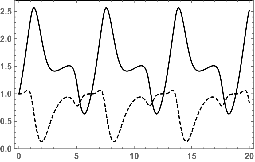
Figure 1: Initial value problem (14), (15). Graphs of the real (bold curve) and imaginary (dashed curve) parts of the coordinate $z_{1}(t)$; period $2\pi$.

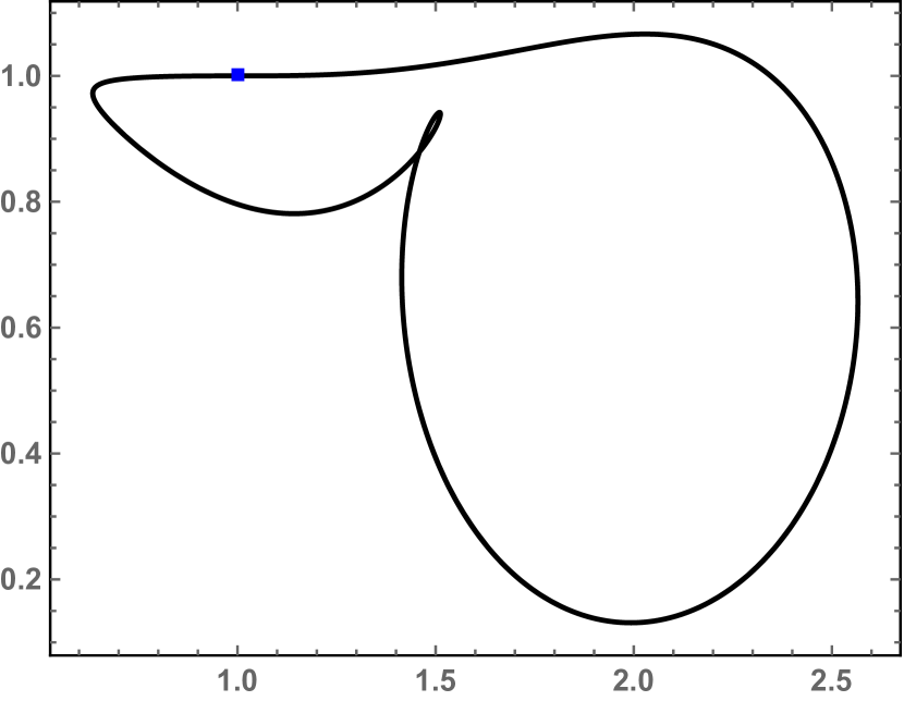
Figure 2: Initial value problem (14), (15). Trajectory, in the complex $z$-plane, of $z_{1}(t)$; period $2\pi$. The square indicates the initial condition $z_{1}(0)=1+\mathbf{i}$.

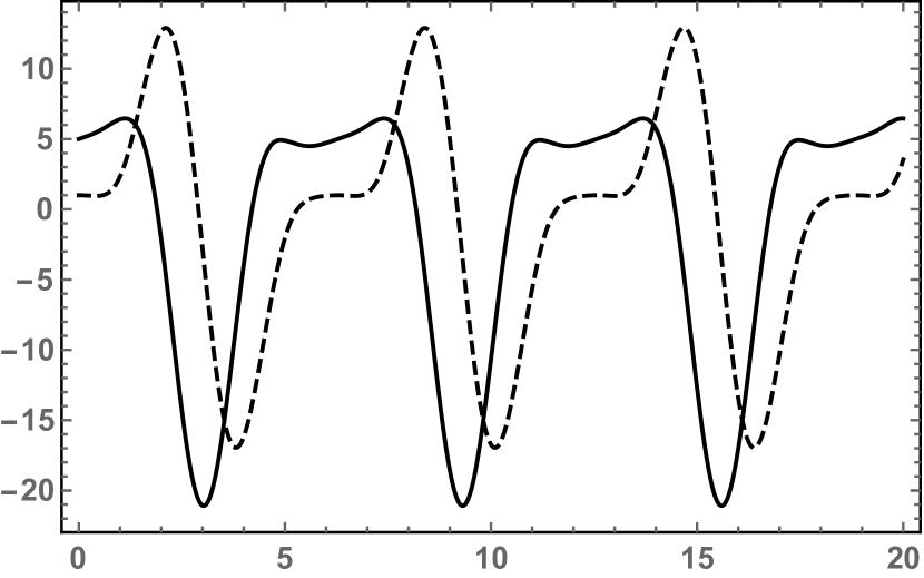
Figure 3: Initial value problem (14), (15). Graphs of the real (bold curve) and imaginary (dashed curve) parts of the coordinate $z_{2}(t)$; period $2\pi$.

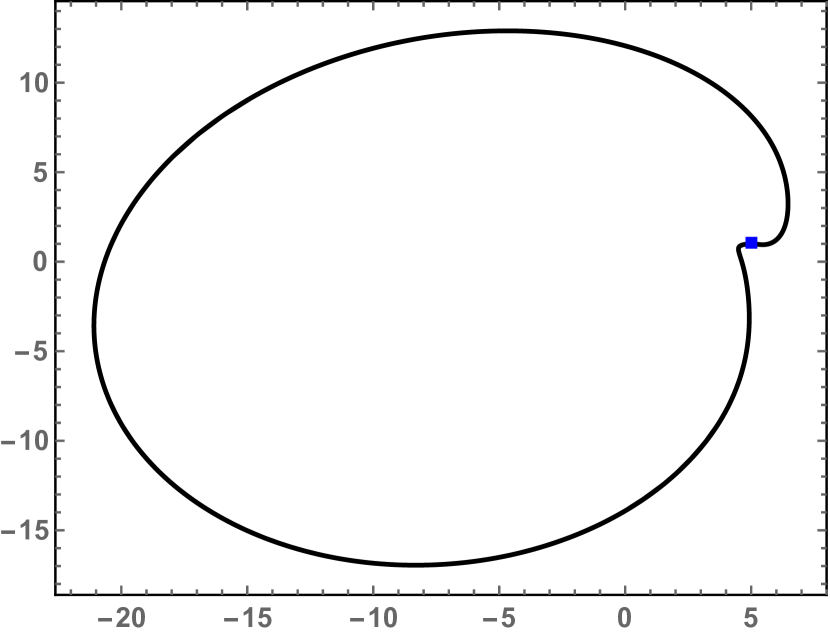
Figure 4: Initial value problem (14), (15). Trajectory, in the complex $z$-plane, of $z_{2}(t)$; period $2\pi$. The square indicates the initial condition $z_{2}(0)=5+\mathbf{i}$.

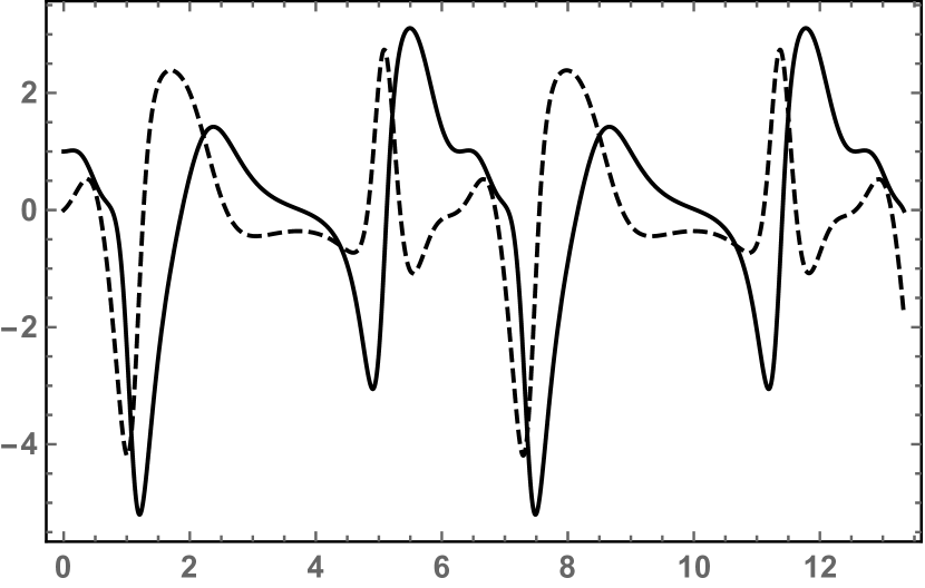
Figure 5: Initial value problem (14), (15). Graphs of the real (bold curve) and imaginary (dashed curve) parts of the coordinate $w_{1}(t)$; period $2\pi$.

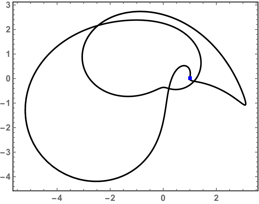
Figure 6: Initial value problem (14), (15). Trajectory, in the complex $z$-plane, of $w_{1}(t)$; period $2\pi$. The square indicates the initial condition $w_{1}(0)=1$.

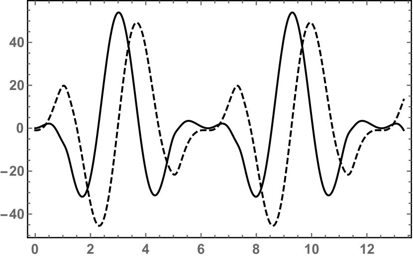
Figure 7: Initial value problem (14), (15). Graphs of the real (bold curve) and imaginary (dashed curve) parts of the coordinate $w_{2}(t)$; period $2\pi$.

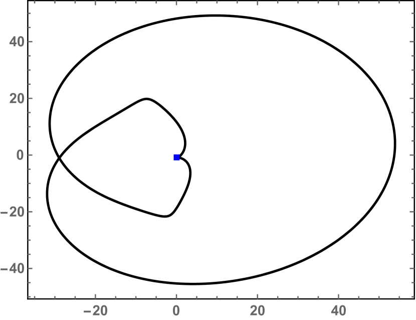
Figure 8: Initial value problem (14), (15). Trajectory, in the complex $z$-plane, of $w_{2}(t)$; period $2\pi$. The square indicates the initial condition $w_{2}(0)=-\mathbf{i}$.

For system (14), (15a), each characteristic equation (22) has the four roots $-\mathbf{i},\mathbf{i},2\mathbf{i},3\mathbf{i}$. Therefore, by (ii) of Remark 2.2, system (14), (15a) is isochronous, see Figures 1, 2, 3, 4, 5, 6, 7, 8 in Appendix B.

Next,we provide plots of the solutions of system (14) with the following values of the parameters $\alpha_{m},\beta_{m},\gamma_{m},\delta_{m}$, $m=1,2,$

$$\alpha_{m}=-3,\beta_{m}=-3,\gamma_{m}=-3,\delta_{m}=-2,m=1,2,$$ (16a)

and the initial conditions

$$z_{1}(0)=-2-\mathbf{i},\dot{z}_{1}(0)=1,z_{2}(0)=2+\mathbf{i},\dot{z}_{2}(0)=1,$$

$$w_{1}(0)=1,\dot{w}_{1}(0)=\mathbf{i},w_{2}(0)=-\mathbf{i},\dot{w}_{2}(0)=1.$$ (16b)

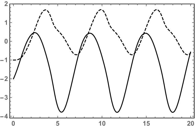
Figure 9: Initial value problem (14), (16). Graphs of the real (bold curve) and imaginary (dashed curve) parts of the coordinate $z_{1}(t)$.

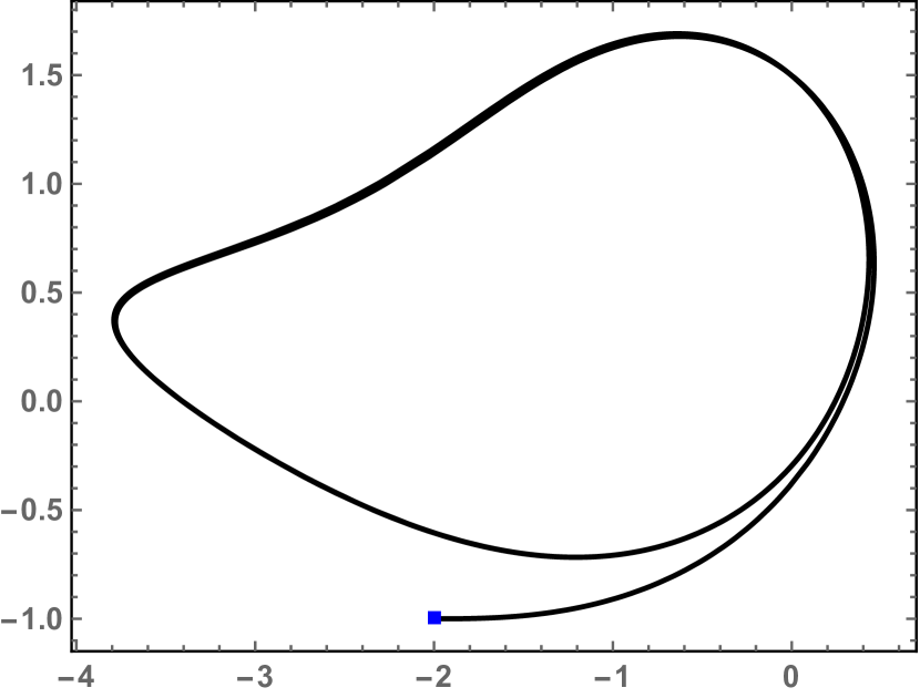
Figure 10: Initial value problem (14), (16). Trajectory, in the complex $z$-plane, of $z_{1}(t)$. The square indicates the initial condition $z_{1}(0)=-2-\mathbf{i}$.

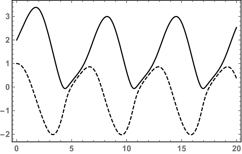
Figure 11: Initial value problem (14), (16). Graphs of the real (bold curve) and imaginary (dashed curve) parts of the coordinate $z_{2}(t)$.

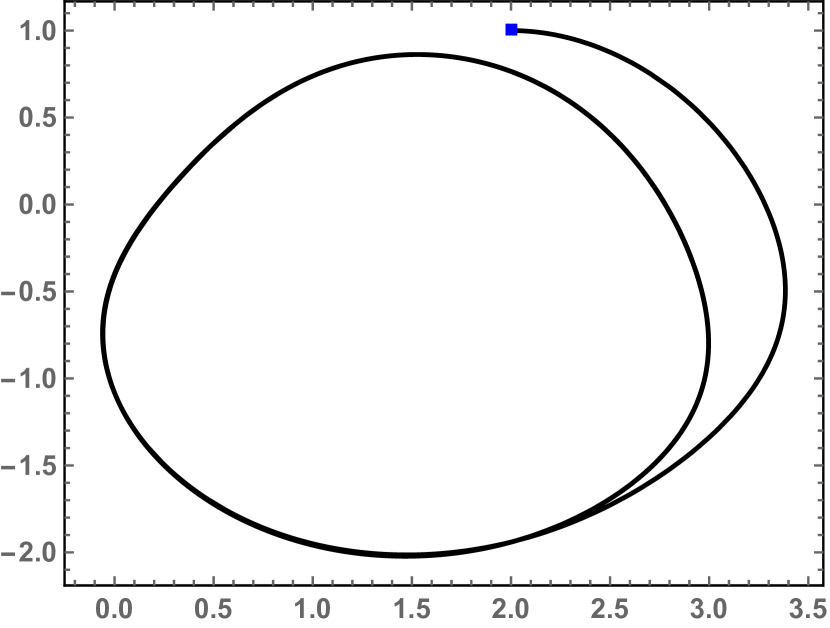
Figure 12: Initial value problem (14), (16). Trajectory, in the complex $z$-plane, of $z_{2}(t)$. The square indicates the initial condition $z_{2}(0)=2+\mathbf{i}$.

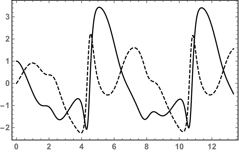
Figure 13: Initial value problem (14), (16). Graphs of the real (bold curve) and imaginary (dashed curve) parts of the coordinate $w_{1}(t)$.

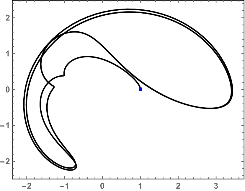
Figure 14: Initial value problem (14), (16). Trajectory, in the complex $z$-plane, of $w_{1}(t)$. The square indicates the initial condition $w_{1}(0)=1$.

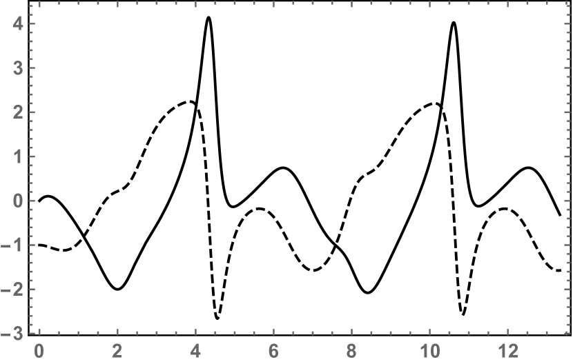
Figure 15: Initial value problem (14), (16). Graphs of the real (bold curve) and imaginary (dashed curve) parts of the coordinate $w_{2}(t)$.

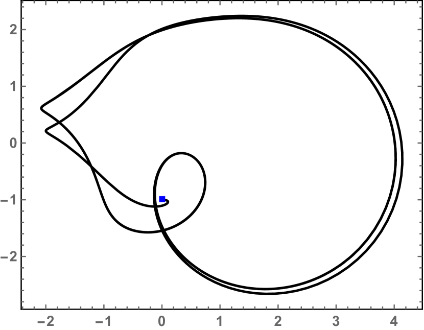
Figure 16: Initial value problem (14), (16). Trajectory, in the complex $z$-plane, of $w_{2}(t)$. The square indicates the initial condition $w_{2}(0)=-\mathbf{i}$.

For the initial value problem (14), (16a), each characteristic equation (22) has the four roots $-\mathbf{i},\mathbf{i},-1,-2$. Therefore, by (i) of Remark 2.2, system (14), (16a) is asymptotically isochronous, see Figures 9, 10, 11, 12, 13, 14, 15, 16 in Appendix B.

Next,we provide plots of the solutions of system (14) with the following values of the parameters $\alpha_{m},\beta_{m},\gamma_{m},\delta_{m}$, $m=1,2$,

$$\alpha_{m}=-3+(\pi-1)\mathbf{i},\beta_{m}=-(\pi+2)+3(\pi-1)\mathbf{i},$$

$$\gamma_{m}=-3\pi+2(\pi-1)\mathbf{i},\delta_{m}=-2\pi,m=1,2,$$ (17a)

and the initial conditions

$$z_{1}(0)=-2-\mathbf{i},\dot{z}_{1}(0)=1,z_{2}(0)=2+\mathbf{i},\dot{z}_{2}(0)=-1,$$

$$w_{1}(0)=\mathbf{i},\dot{w}_{1}(0)=1,w_{2}(0)=-\mathbf{i},\dot{w}_{2}(0)=-1.$$ (17b)

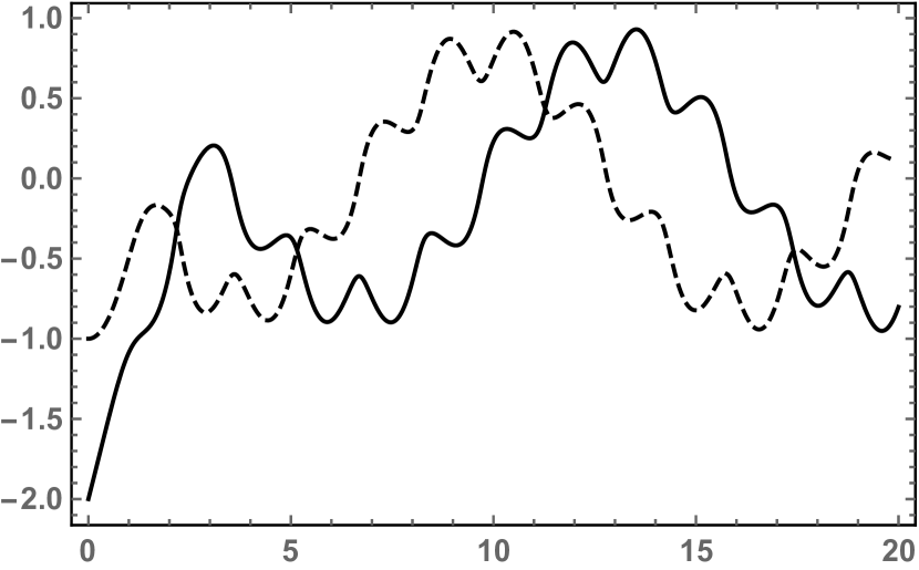
Figure 17: Initial value problem (14), (17). Graphs of the real (bold curve) and imaginary (dashed curve) parts of the coordinate $z_{1}(t)$.

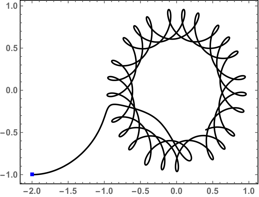
Figure 18: Initial value problem (14), (17). Trajectory, in the complex $z$-plane, of $z_{1}(t)$. The square indicates the initial condition $z_{1}(0)=-2-\mathbf{i}$.

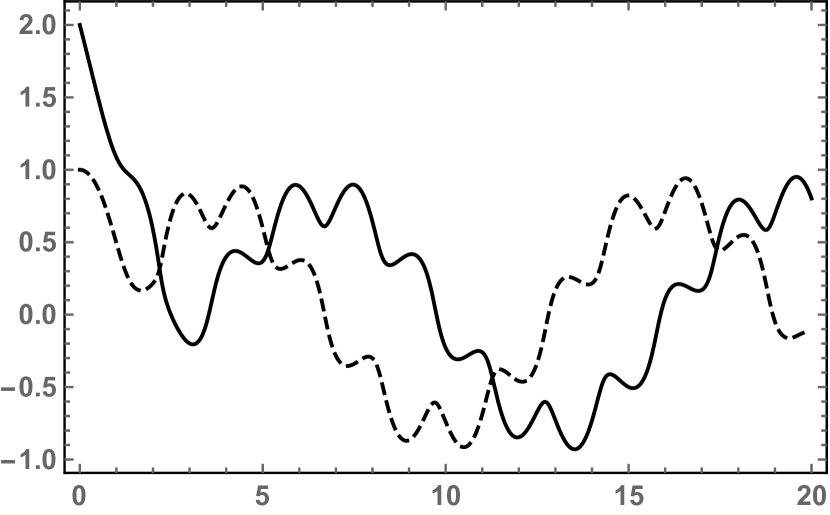
Figure 19: Initial value problem (14), (17). Graphs of the real (bold curve) and imaginary (dashed curve) parts of the coordinate $z_{2}(t)$.

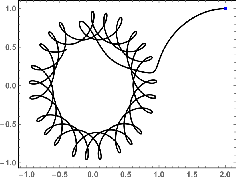
Figure 20: Initial value problem (14), (17). Trajectory, in the complex $z$-plane, of $z_{2}(t)$. The square indicates the initial condition $z_{2}(0)=2+\mathbf{i}$.

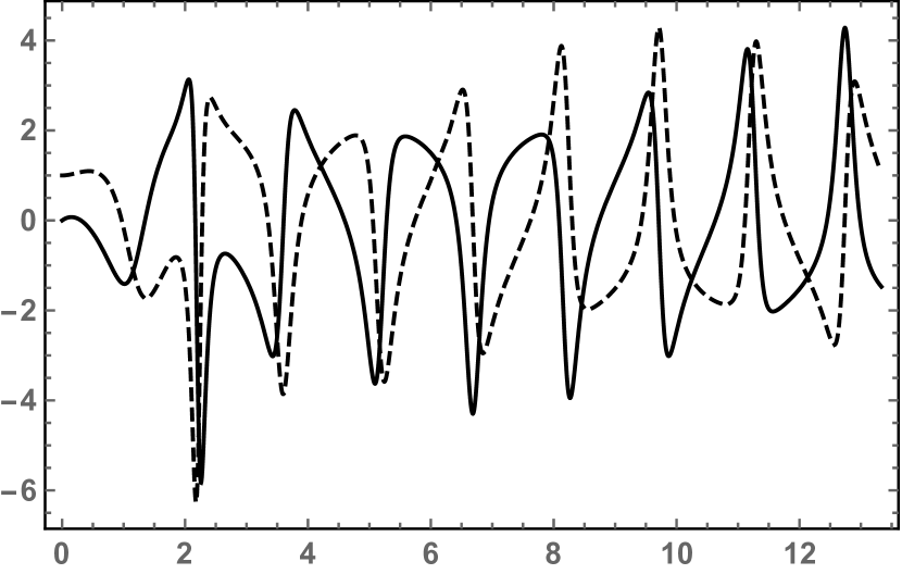
Figure 21: Initial value problem (14), (17). Graphs of the real (bold curve) and imaginary (dashed curve) parts of the coordinate $w_{1}(t)$.

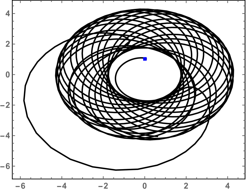
Figure 22: Initial value problem (14), (17). Trajectory, in the complex $z$-plane, of $w_{1}(t)$. The square indicates the initial condition $w_{1}(0)=\mathbf{i}$.

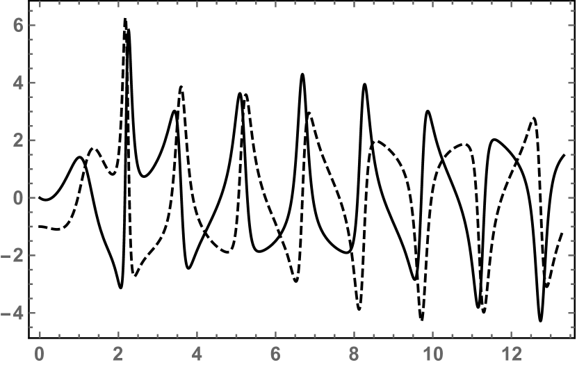
Figure 23: Initial value problem (14), (17). Graphs of the real (bold curve) and imaginary (dashed curve) parts of the coordinate $w_{2}(t)$.

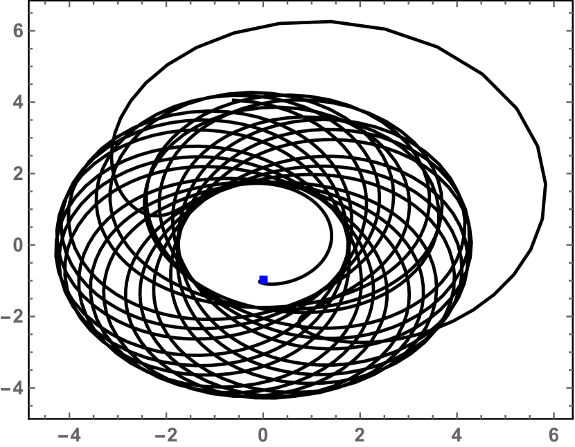
Figure 24: Initial value problem (14), (17). Trajectory, in the complex $z$-plane, of $w_{2}(t)$. The square indicates the initial condition $w_{2}(0)=-\mathbf{i}$.

For system (14), (17a), each characteristic equation (22) has the four roots $-\mathbf{i},\pi\mathbf{i},-1,-2$. Therefore, by (i) of Remark 2.2, system (14), (17a) is asymptotically multiply periodic, see Figures 17, 18, 19, 20, 21, 22, 23, 24 in Appendix B.

Next,we provide plots of the solutions of system (14) with the following values of the parameters $\alpha_{m},\beta_{m},\gamma_{m},\delta_{m}$, $m=1,2$,

$$\alpha_{1}=0.222+1.4\mathbf{i},\beta_{1}=0.41208-0.2208\mathbf{i},$$

$$\gamma_{1}=-0.038436-0.018968\mathbf{i},\delta_{1}=0.000866464+0.0010224\mathbf{i},$$

$$\alpha_{2}=0.172+1.1\mathbf{i},\beta_{2}=0.06952-0.1512\mathbf{i},$$

$$\gamma_{2}=-0.006696+0.026376\mathbf{i},\delta_{2}=0.000104896-0.00047584\mathbf{i},$$ (18a)

and the initial conditions

$$z_{1}(0)=-2+3\mathbf{i},\dot{z}_{1}(0)=7,z_{2}(0)=3+2\mathbf{i},\dot{z}_{2}(0)=-5,$$

$$w_{1}(0)=2+4.2\mathbf{i},\dot{w}_{1}(0)=4.5,w_{2}(0)=3.1\mathbf{i},\dot{w}_{2}(0)=2.4.$$ (18b)

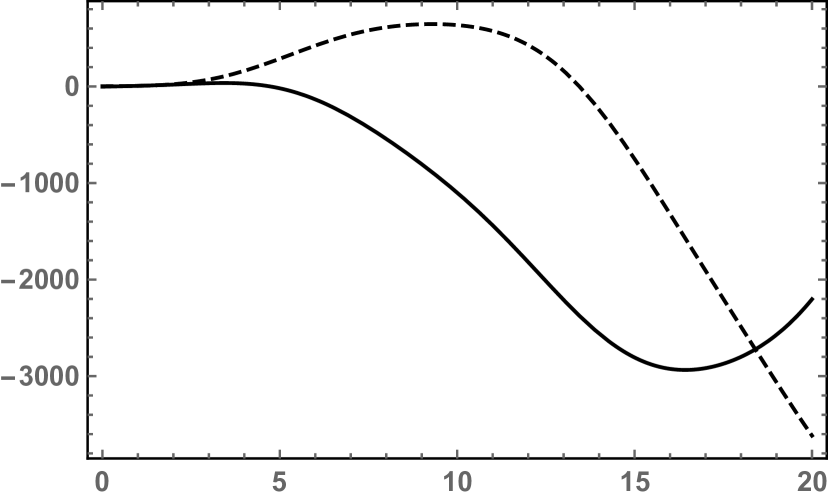
Figure 25: Initial value problem (14), (18). Graphs of the real (bold curve) and imaginary (dashed curve) parts of the coordinate $z_{1}(t)$.

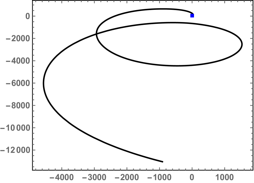
Figure 26: Initial value problem (14), (18). Trajectory, in the complex $z$-plane, of $z_{1}(t)$. The square indicates the initial condition $z_{1}(0)=-2+3\mathbf{i}$.

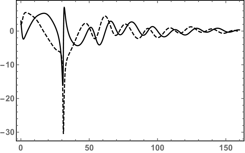
Figure 27: Initial value problem (14), (18). Graphs of the real (bold curve) and imaginary (dashed curve) parts of the coordinate $z_{2}(t)$.

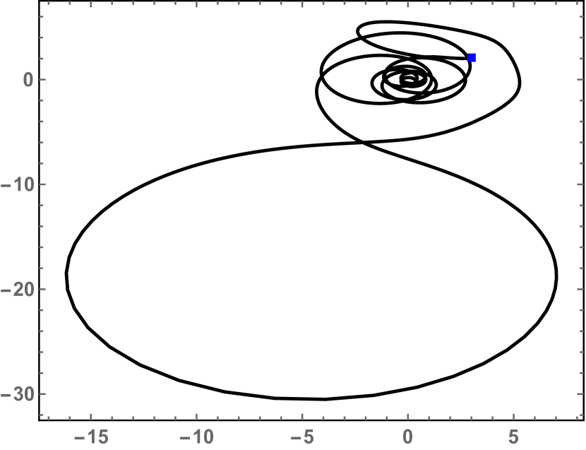
Figure 28: Initial value problem (14), (18). Trajectory, in the complex $z$-plane, of $z_{2}(t)$. The square indicates the initial condition $z_{2}(0)=3+2\mathbf{i}$.

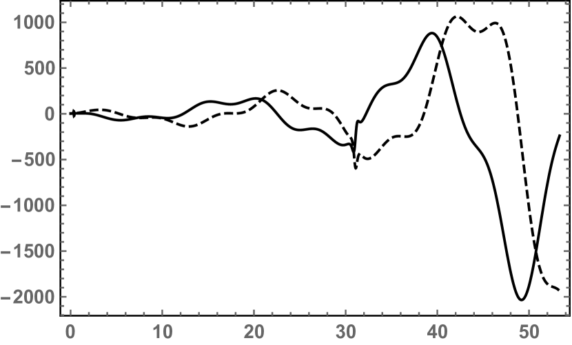
Figure 29: Initial value problem (14), (18). Graphs of the real (bold curve) and imaginary (dashed curve) parts of the coordinate $w_{1}(t)$.

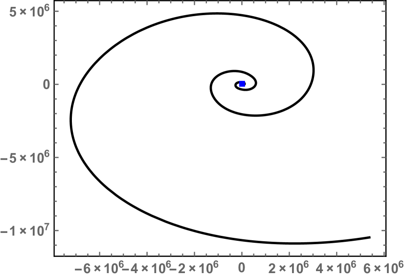
Figure 30: Initial value problem (14), (18). Trajectory, in the complex $z$-plane, of $w_{1}(t)$. The square indicates the initial condition $w_{1}(0)=2+4.2\mathbf{i}$.

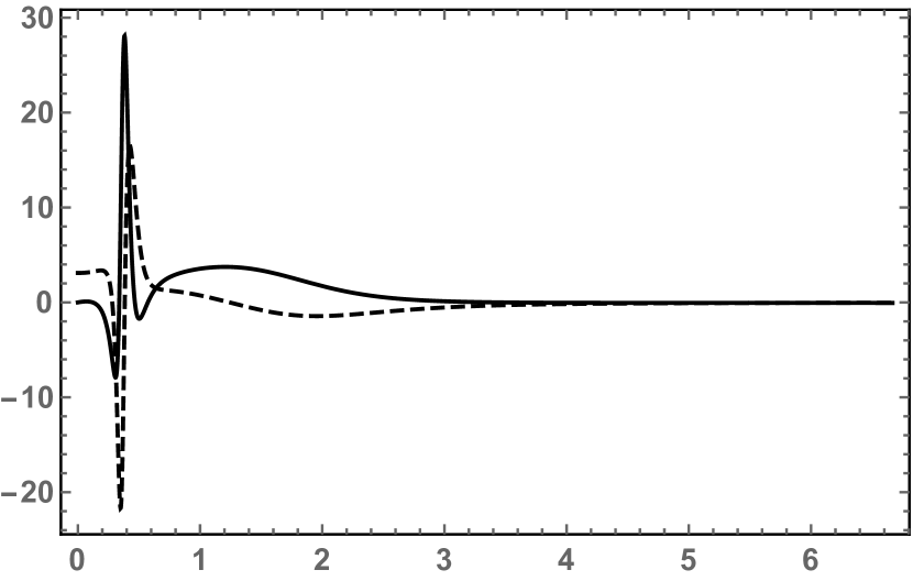
Figure 31: Initial value problem (14), (18). Graphs of the real (bold curve) and imaginary (dashed curve) parts of the coordinate $w_{2}(t)$.

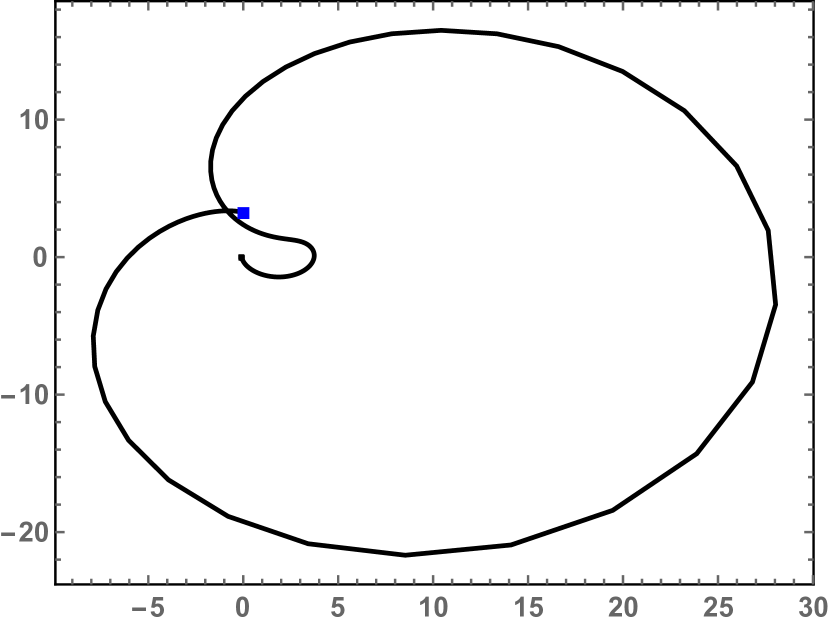
Figure 32: Initial value problem (14), (18). Trajectory, in the complex $z$-plane, of $w_{2}(t)$. The square indicates the initial condition $w_{2}(0)=3.1\mathbf{i}$.

For system (14), (18a), the characteristic equation (22) for $m=1$ has the four roots $0.04,0.062+\mathbf{i},0.08+0.3\mathbf{i},0.04+0.1\mathbf{i}$ and the characteristic equation (22) for $m=2$ has the four roots $0.02,0.032+\mathbf{i},0.06-0.1\mathbf{i},0.06+0.2\mathbf{i}$. In agreement with (iii) of Remark 2.2, the components $z_{1}$ and $w_{1}$ of the solution of system (14), (18a) exhibit scattering phenomena, see Figures 25, 26, 27, 28, 29, 30, 31, 32 in Appendix B. From these figures, it is clear that $z_{1}(t)$ diverges exponentially as $t\to\infty$ (and of course $w_{1}(t)$ features the same behavior), while $z_{2}(t)$ and $w_{2}(t)$ converge to zero as $t\to\infty$, which is consistent with the behavior of the zeros of polynomials whose coefficients depend on $t$ exponentially, as reported in Appendix G of [7].

Example 2. If $N=3$, system (8) reduces to

$$\ddot{z}_{1}=w_{1},\ddot{z}_{2}=w_{2},\ddot{z}_{3}=w_{3},$$

$$\ddot{w}_{1}=\frac{4\dot{w}_{1}\dot{z}_{2}+4\dot{w}_{2}\dot{z}_{1}+6w_{1}w_{2}}{z_{1}-z_{2}}+\frac{4\dot{w}_{1}\dot{z}_{3}+4\dot{w}_{3}\dot{z}_{1}+6w_{1}w_{3}}{z_{1}-z_{3}}$$

$$-\frac{1}{(z_{1}-z_{2})(z_{1}-z_{3})}\Bigg{\{}12\left[w_{1}\dot{z}_{2}\dot{z}_{3}+\dot{z}_{1}(w_{2}\dot{z}_{3}+w_{3}\dot{z}_{2})\right]+z_{1}^{2}K_{1}(\vec{z},\dot{\vec{z}},\vec{w},\dot{\vec{w}})$$

$$+z_{1}K_{2}(\vec{z},\dot{\vec{z}},\vec{w},\dot{\vec{w}})+K_{3}(\vec{z},\dot{\vec{z}},\vec{w},\dot{\vec{w}})\Bigg{\}},$$

$$\ddot{w}_{2}=\frac{4\dot{w}_{2}\dot{z}_{1}+4\dot{w}_{1}\dot{z}_{2}+6w_{1}w_{2}}{z_{2}-z_{1}}+\frac{4\dot{w}_{2}\dot{z}_{3}+4\dot{w}_{3}\dot{z}_{2}+6w_{2}w_{3}}{z_{2}-z_{3}}$$

$$-\frac{1}{(z_{2}-z_{1})(z_{2}-z_{3})}\Bigg{\{}12\left[w_{2}\dot{z}_{1}\dot{z}_{3}+\dot{z}_{2}(w_{1}\dot{z}_{3}+w_{3}\dot{z}_{1})\right]+z_{2}^{2}K_{1}(\vec{z},\dot{\vec{z}},\vec{w},\dot{\vec{w}})$$

$$+z_{2}K_{2}(\vec{z},\dot{\vec{z}},\vec{w},\dot{\vec{w}})+K_{3}(\vec{z},\dot{\vec{z}},\vec{w},\dot{\vec{w}})\Bigg{\}},$$

$$\ddot{w}_{3}=\frac{4\dot{w}_{3}\dot{z}_{1}+4\dot{w}_{1}\dot{z}_{3}+6w_{1}w_{3}}{z_{3}-z_{1}}+\frac{4\dot{w}_{3}\dot{z}_{2}+4\dot{w}_{2}\dot{z}_{3}+6w_{2}w_{3}}{z_{3}-z_{2}}$$

$$-\frac{1}{(z_{3}-z_{1})(z_{3}-z_{2})}\Bigg{\{}12\left[w_{3}\dot{z}_{1}\dot{z}_{2}+\dot{z}_{3}(w_{1}\dot{z}_{2}+w_{2}\dot{z}_{1})\right]+z_{3}^{2}K_{1}(\vec{z},\dot{\vec{z}},\vec{w},\dot{\vec{w}})$$

$$+z_{3}K_{2}(\vec{z},\dot{\vec{z}},\vec{w},\dot{\vec{w}})+K_{3}(\vec{z},\dot{\vec{z}},\vec{w},\dot{\vec{w}})\Bigg{\}},$$

where

$$K_{1}(\vec{z},\dot{\vec{z}},\vec{w},\dot{\vec{w}})=-\Big{[}\alpha_{1}(\dot{w}_{1}+\dot{w}_{2}+\dot{w}_{3})+\beta_{1}(w_{1}+w_{2}+w_{3})$$

$$+\gamma_{1}(\dot{z}_{1}+\dot{z}_{2}+\dot{z}_{3})+\delta_{1}(z_{1}+z_{2}+z_{3}),$$ (19b)

$$K_{2}(\vec{z},\dot{\vec{z}},\vec{w},\dot{\vec{w}})=\alpha_{2}\Big{[}\dot{w}_{1}(z_{2}+z_{3})+\dot{w}_{2}(z_{1}+z_{3})+\dot{w}_{3}(z_{1}+z_{2})+2w_{1}(\dot{z}_{2}+\dot{z}_{3})$$

$$+2w_{2}(\dot{z}_{1}+\dot{z}_{3})+2w_{3}(\dot{z}_{1}+\dot{z}_{2})+\dot{z}_{1}(w_{2}+w_{3})+\dot{z}_{2}(w_{1}+w_{3})+\dot{z}_{3}(w_{1}+w_{2})\Big{]}$$

$$+\beta_{2}\Big{[}w_{1}(z_{2}+z_{3})+w_{2}(z_{1}+z_{3})+w_{3}(z_{1}+z_{2})+\dot{z}_{1}(\dot{z}_{2}+\dot{z}_{3})+\dot{z}_{2}(\dot{z}_{1}+\dot{z}_{3})$$

$$+\dot{z}_{3}(\dot{z}_{1}+\dot{z}_{2})\Big{]}+\gamma_{2}\Big{[}\dot{z}_{1}(z_{2}+z_{3})+\dot{z}_{2}(z_{1}+z_{3})+\dot{z}_{3}(z_{1}+z_{2})\Big{]}$$

$$+\delta_{2}(z_{1}z_{2}+z_{1}z_{3}+z_{2}z_{3}),$$ (19c)

$$K_{3}(\vec{z},\dot{\vec{z}},\vec{w},\dot{\vec{w}})=-\Bigg{\{}\alpha_{3}\Big{[}\dot{w}_{1}z_{2}z_{3}+\dot{w}_{2}z_{1}z_{3}+\dot{w}_{3}z_{1}z_{2}+2w_{1}(\dot{z}_{2}z_{3}+z_{2}\dot{z}_{3})$$

$$+2w_{2}(\dot{z}_{1}z_{3}+z_{1}\dot{z}_{3})+2w_{3}(\dot{z}_{1}z_{2}+z_{1}\dot{z}_{2})+\dot{z}_{1}(w_{2}z_{3}+2\dot{z}_{2}\dot{z}_{3}+z_{2}w_{3})$$

$$+\dot{z}_{2}(w_{1}z_{3}+2\dot{z}_{1}\dot{z}_{3}+z_{1}w_{3})+\dot{z}_{3}(w_{1}z_{2}+2\dot{z}_{1}\dot{z}_{2}+z_{1}w_{2})\Big{]}$$

$$+\beta_{3}\Big{[}w_{1}z_{2}z_{3}+w_{2}z_{1}z_{3}+w_{3}z_{1}z_{2}+\dot{z}_{1}(\dot{z}_{2}z_{3}+z_{2}\dot{z}_{3})+\dot{z}_{2}(\dot{z}_{1}z_{3}+z_{1}\dot{z}_{3})$$

$$+\dot{z}_{3}(\dot{z}_{1}z_{2}+z_{1}\dot{z}_{2})\Big{]}+\gamma_{3}\Big{[}\dot{z}_{1}z_{2}z_{3}+z_{1}\dot{z}_{2}z_{3}+z_{1}z_{2}\dot{z}_{3}\Big{]}+\delta_{3}z_{1}z_{2}z_{3}\Bigg{\}}.$$ (19d)

In Appendix B we provide plots of the solutions of system (19) with the following values of the parameters $\alpha_{m},\beta_{m},\gamma_{m},\delta_{m}$, $m=1,2,3,$

$$\alpha_{1}=5\mathbf{i},\beta_{1}=5,\gamma_{1}=5\mathbf{i},\delta_{1}=6,$$

$$\alpha_{2}=4\mathbf{i},\beta_{2}=-1,\gamma_{2}=16\mathbf{i},\delta_{2}=12,$$

$$\alpha_{3}=0,\beta_{3}=-5,\gamma_{3}=0,\delta_{3}=-4,$$

(20a)

and the initial conditions

$$z_{1}(0)=-1.45+1.1\mathbf{i},\dot{z}_{1}(0)=0.9,$$

$$z_{2}(0)=5.1+0.8\mathbf{i},\dot{z}_{2}(0)=1.2,$$

$$z_{3}(0)=2.5-0.2\mathbf{i},\dot{z}_{3}(0)=-1.04,$$

$$w_{1}(0)=1.23,\dot{w}_{1}(0)=0.84\mathbf{i},$$

$$w_{2}(0)=-2.26\mathbf{i},\dot{w}_{2}(0)=2.16,$$

$$w_{3}(0)=1.32\mathbf{i},\dot{w}_{3}(0)=-1.12.$$ (20b)

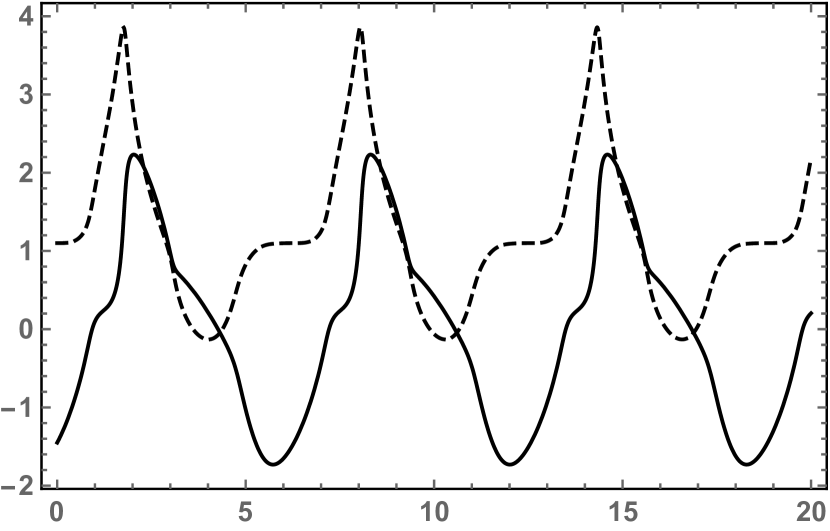
Figure 33: Initial value problem (19), (20). Graphs of the real (bold curve) and imaginary (dashed curve) parts of the coordinate $z_{1}(t)$.

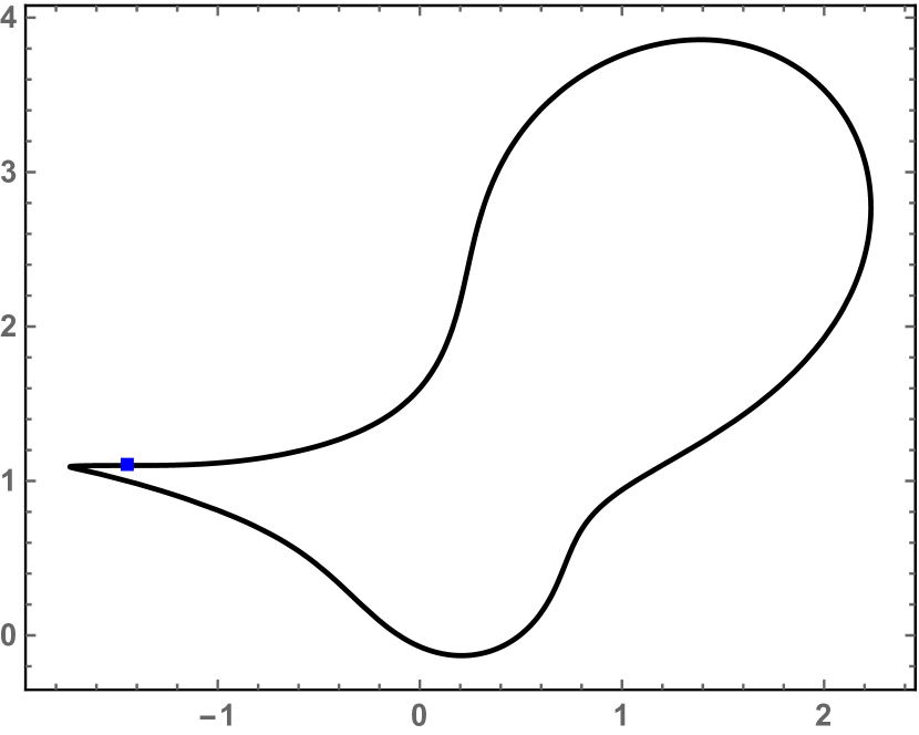
Figure 34: Initial value problem (19), (20). Trajectory, in the complex $z$-plane, of $z_{1}(t)$; period $2\pi$. The square indicates the initial condition $z_{1}(0)=-1.45+1.1\mathbf{i}$.

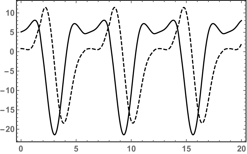
Figure 35: Initial value problem (19), (20). Graphs of the real (bold curve) and imaginary (dashed curve) parts of the coordinate $z_{2}(t)$.

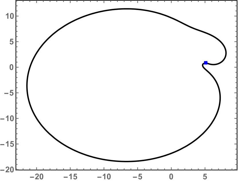
Figure 36: Initial value problem (19), (20). Trajectory, in the complex $z$-plane, of $z_{2}(t)$; period $4\pi$. The square indicates the initial condition $z_{2}(0)=5.1+0.8\mathbf{i}$.

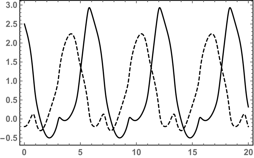
Figure 37: Initial value problem (19), (20). Graphs of the real (bold curve) and imaginary (dashed curve) parts of the coordinate $z_{3}(t)$.

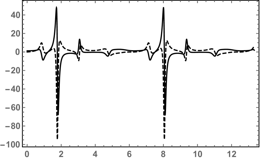
Figure 39: Initial value problem (19), (20). Graphs of the real (bold curve) and imaginary (dashed curve) parts of the coordinate $w_{1}(t)$.

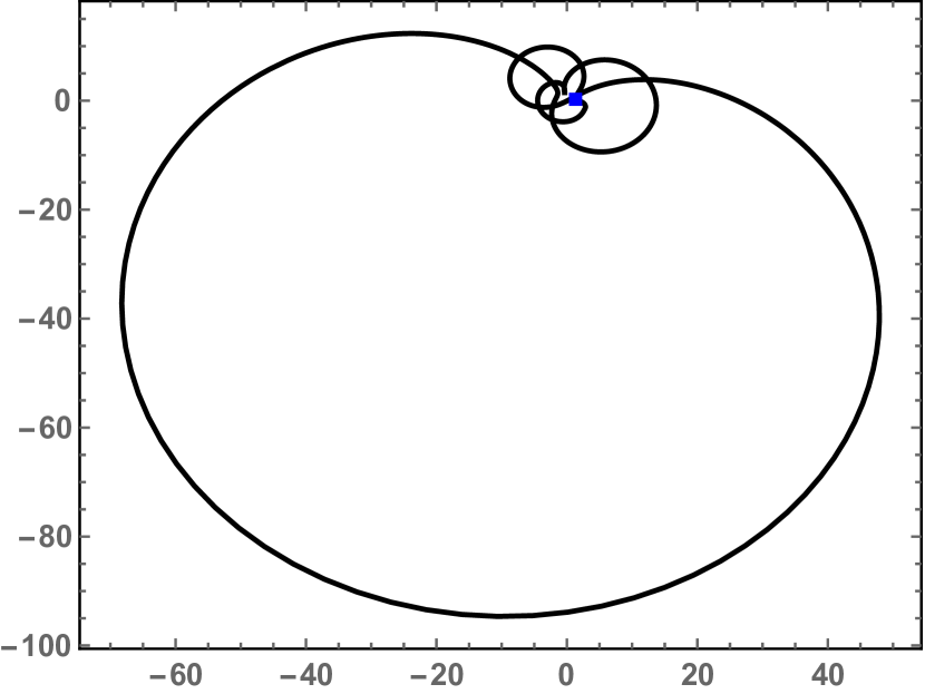
Figure 40: Initial value problem (19), (20). Trajectory, in the complex $z$-plane, of $w_{1}(t)$; period $2\pi$. . The square indicates the initial condition $w_{1}(0)=1.23$.

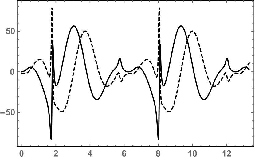
Figure 41: Initial value problem (19), (20). Graphs of the real (bold curve) and imaginary (dashed curve) parts of the coordinate $w_{2}(t)$.

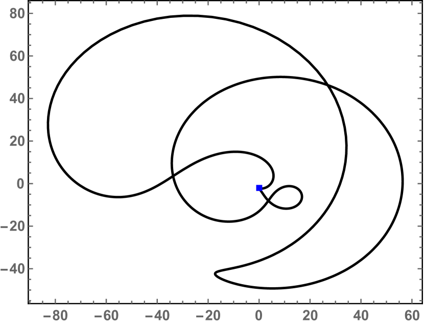
Figure 42: Initial value problem (19), (20). Trajectory, in the complex $z$-plane, of $w_{2}(t)$; period $4\pi$. The square indicates the initial condition $w_{2}(0)=-2.26\mathbf{i}$.

For system (19), (20a), the characteristic equation (22) for $m=1$ has the four roots $-\mathbf{i},\mathbf{i},2\mathbf{i},3\mathbf{i}$, the characteristic equation (22) for $m=2$ has the four roots $-2\mathbf{i},\mathbf{i},2\mathbf{i},3\mathbf{i}$ and the characteristic equation (22) for $m=3$ has the four roots $-2\mathbf{i},-\mathbf{i},\mathbf{i},2\mathbf{i}$,. Therefore, by (ii) of Remark 2.2, system (19), (20a) is isochronous, see Figures 33, 34, 35, 36, 37, 38, 39, 40, 41, 42 in Appendix B.

3 New solvable dynamical systems and their solutions

In this section we indicate how to identify endless sequences of solvable dynamical systems describing the motion in the complex $z$-plane of point-particles interacting among themselves with certain forces depending on their positions and velocities. Let us reiterate that a many-body model is considered solvable if the configuration of the system at any arbitrary time $t$ can be obtained—from any given initial data: the initial positions and velocities of the $N$ particles in the complex $z$-plane—by algebraic operations, such as finding the zeros of an explicitly known time-dependent polynomial.

Remark 3.1. Note however that knowledge of the configuration of the many-body system at time $t$, with the (generally complex) values of its coordinates given as the unordered set of the zeros of a known polynomial, does not allow to identify the specific coordinate that has evolved over time from the assignment of its specific initial position and velocity; this additional information can only be gained by following over time the evolution of the system, either by integrating numerically the equations of motion, or by identifying the configurations of the system at a sequence of time intervals sufficiently close to each other so as to guarantee the identification by continuity of the trajectory of each particle (or at least of the specific particle under consideration). But these additional operations need not be performed with great accuracy, even when one wishes the final configuration—including the identity of each particle—to be known with much greater accuracy.

Likewise—in the case of systems which have been identified as isochronous because their solution is provided by the zeros of a time-dependent polynomial which is itself periodic in time with period, say, $T$—an analogous procedure must be followed to ascertain whether the period of the time evolution of a specific particle is $T$, or $pT$ (with $p$ a positive integer), due to the possibility of a $T$-periodic exchange of the correspondence between the zeros of the polynomial and the particle identities (for a general discussion of this possibility in a specific context see [8]). $\blacksquare$

The key formulas for the following developments are the identities (3), relating the time evolution of the zeros $z_{n}\left(t\right)$ of a time-dependent (monic) polynomial to that of the coefficients $c_{m}\left(t\right)$ of the same polynomial, as well as the relations (4) respectively (7) expressing the coefficients $c_{m}\left(t\right)$ of a monic polynomial respectively their time derivatives in terms of the zeros of the same polynomial and their time derivatives.

In this paper we restrict for simplicity attention to the case of a linear decoupled evolution of the coefficients $c_{m}\left(t\right)$, namely we assume that these $N$ coefficients of the time-dependent polynomial (2) evolve in time according to the following system of ODEs,

$$\ddddot{c}_{m}=\alpha_{m}~{}\dddot{c}_{m}+\beta_{m}~{}\ddot{c}_{m}+\gamma_{m}~{}\dot{c}_{m}+\delta_{m}~{},$$ (21)

where the parameters $\alpha_{m},~{}\beta_{m},~{}\gamma_{m},~{}\delta_{m}$ are $4N$ generic complex numbers such that for each $m$, the characteristic equation

$$\left(\lambda_{m}\right)^{4}=\alpha_{m}~{}\left(\lambda_{m}\right)^{3}+\beta_{m}~{}\left(\lambda_{m}\right)^{2}+\gamma_{m}~{}\lambda_{m}+\delta_{m}~{},$$ (22)

has four distinct roots $\lambda_{m,k},k=1,2,3,4$ (see below). It is then plain that the general solution of this system reads as follows :

$$c_{m}\left(t\right)=\sum_{k=1}^{4}\left[b_{m}^{\left(k\right)}~{}\exp\left(\lambda_{m,k}~{}t\right)\right]~{}.$$ (23a)

The $$4N \lambda_{m,k} 4 k$$ numbers , labeled by the values of the index , are denoted as follows:

$$\lambda_{m,k}=-a_{m}^{\left(k\right)}+\mathbf{i}~{}\omega_{m}^{\left(k\right)}~{},~{}~{}~{}k=1,2,3,4~{},$$ (23b)

introducing thereby the $$8N a_{m}^{\left(1\right)} a_{m}^{\left(2\right)} a_{m}^{\left(3\right)} a_{m}^{\left(4\right)} \omega_{m}^{\left(1\right)} \omega_{m}^{\left(2\right)} \omega_{m}^{\left(3\right)} \omega_{m}^{\left(4\right)}$$ real parameters , , , , , , , , implying that the general solution (23a) can be equivalently written as (10).

Remark 3.2. The fourth-degree algebraic equations (22) could be explicitly solved, but the formulas expressing, for every value of the index $m$, the $4$ exponents $\lambda_{m,k}$ in terms of the $4$ parameters $\alpha_{m}$,$~{}\beta_{m}$, $\gamma_{m}$,$~{}\delta_{m}$ are too complicated to be of much use. The converse formulas, expressing, for every value of the index $m$, the $4$ parameters $\alpha_{m}$,$~{}\beta_{m}$, $\gamma_{m}$,$~{}\delta_{m}$ in terms of the $4$ exponents $\lambda_{m,k}$, or rather their real and imaginary parts, see (23b), are instead rather neat, see (9). $\blacksquare$

As for the $4N$ numbers $b_{m}^{\left(k\right)}$ in (23a), they are a priori arbitrary; but can of course be determined in terms of the initial data (thereby solving the initial value problem of the dynamical system (21)) by solving, for each of the $N$ values of the index $m$, the following system of $4$ linear algebraic equations,

$$\sum_{k=1}^{4}\left[b_{m}^{\left(k\right)}~{}\left(\lambda_{m,k}\right)^{s}\right]=\left.\frac{d^{s}c_{m}\left(t\right)}{dt^{s}}\right|_{t=0}~{},~{}~{}~{}s=0,1,2,3~{}.$$ (23c)

Remark 3.3. It is plain that one could have considered, instead of the system of $N$ linear decoupled ODEs (21), the more general system of $N$ linear coupled ODEs

$$\ddddot{c}_{m}=\sum_{n=1}^{N}\left(A_{mn}~{}\dddot{c}_{n}+B_{mn}~{}\ddot{c}_{n}+C_{mn}~{}\dot{c}_{n}+D_{mn}~{}c_{n}\right)~{},$$ (24)

which is of course also solvable by algebraic operations, while featuring more arbitrary constants ($4N^{2}$ instead than $4N$). $\blacksquare$

The solvable character of the dynamical system characterized by the following $N$ coupled nonlinear ODEs to be satisfied by the $N$ dependent variables $z_{n}\equiv z_{n}\left(t\right)$ is then clearly implied by the formula (3d):

$$\ddddot{z}_{n}=\sum_{\ell=1}^{N}{}^{\prime}\left(\frac{4~{}\dddot{z}_{n}~{}\dot{z}_{\ell}+4~{}\dddot{z}_{\ell}~{}\dot{z}_{n}+6~{}\ddot{z}_{n}~{}\ddot{z}_{\ell}}{z_{n}-z_{\ell}}\right)$$

$$-6~{}\sum_{\ell_{1},\ell_{2}=1}^{N}{}^{\prime}\left[\frac{\ddot{z}_{n}~{}\dot{z}_{\ell_{1}}~{}\dot{z}_{\ell_{2}}+2~{}\ddot{z}_{\ell_{1}}~{}\dot{z}_{n}~{}\dot{z}_{\ell_{2}}}{\left(z_{n}-z_{\ell_{1}}\right)~{}\left(z_{n}-z_{\ell_{2}}\right)}\right]$$

$$+4~{}\sum_{\ell_{1},\ell_{2},~{}\ell_{3}=1}^{N}{}^{\prime}\left[\frac{\dot{z}_{n}~{}\dot{z}_{\ell_{1}}~{}\dot{z}_{\ell_{2}}~{}\dot{z}_{\ell_{3}}}{\left(z_{n}-z_{\ell_{1}}\right)~{}\left(z_{n}-z_{\ell_{2}}\right)~{}\left(z_{n}-z_{\ell_{3}}\right)}\right]-\left[\prod\limits_{\ell=1,~{}\ell\neq n}^{N}\left(z_{n}-z_{\ell}\right)^{-1}\right]\cdot$$

$$\cdot\sum_{m=1}^{N}\left[\left(\alpha_{m}~{}\dddot{c}_{m}+\beta_{m}~{}\ddot{c}_{m}+\gamma_{m}~{}\dot{c}_{m}+\delta_{m}~{}c_{m}\right)~{}\left(z_{n}\right)^{N-m}\right]~{}.$$ (25)

In the last term the $4$ quantities $\dddot{c}_{m}$, $\ddot{c}_{m}$, $\dot{c}_{m}$ and $c_{m}$ must of course be expressed in terms of the dependent variables $z_{n}$ and their time-derivatives by the formulas (7) and (4) (of course with (1)). Indeed the solution of this dynamical system—(25) with (7) and (4)—is clearly provided by the $N$ zeros of the monic polynomial (2b) where the coefficients $c_{m}\left(t\right)$ are given by the formulas (10)—with the coefficients $b_{m}^{\left(k\right)}$ appearing there expressed, as indicated above after eq. (23c), in terms of the initial data $c_{m}\left(0\right),$ $\dot{c}_{m}\left(0\right),$ $\ddot{c}_{m}\left(0\right),$ $\dddot{c}_{m}\left(0\right),$ themselves expressed in terms of the initial data $z_{n}\left(0\right),$ $\dot{z}_{n}\left(0\right),$ $\ddot{z}_{n}\left(0\right),$ $\dddot{z}_{n}\left(0\right)$ via the formulas (4) and (7) at $t=0$.

Remark 3.4. If in the (last term in the) right-hand side of (25) any one of the parameters $\alpha_{m},~{}\beta_{m},~{}\gamma_{m},~{}\delta_{m}$ is independent of the index $m,$ say $\beta_{m}=\beta$, then the corresponding term can be replaced by a simpler expression via the appropriate identity (3), implying, say,

$$\left[\prod\limits_{\ell=1,~{}\ell\neq n}^{N}\left(z_{n}-z_{\ell}\right)^{-1}\right]~{}\sum_{m=1}^{N}\left[\beta~{}\ddot{c}_{m}~{}\left(z_{n}\right)^{N-m}\right]=\beta~{}\left[\ddot{z}_{n}-\sum_{\ell=1}^{N}{}^{\prime}\left(\frac{2~{}\dot{z}_{n}~{}\dot{z}_{\ell}}{z_{n}-z_{\ell}}\right)\right]~{},$$ (26)

see (3b). $\blacksquare$

4 Outlook

The findings reported in this paper suggest further developments, which ourselves or others might pursue and report in future publications.

One direction of future research is the exploration of the solvable dynamical systems and many-body problems of Newtonian type that are obtained by iterating the type of approach described above, along the lines discussed in [4].

It would also be of interest to obtain generalizations of the identities (3) to derivatives of order higher than 4, indeed hopefully of arbitrary order.

And of course further explorations are appealing of the detailed behaviors of the solutions of the dynamical systems obtained via this approach, as well as—in the case of solvable many-body problems of Newtonian type allowing a Hamiltonian formulation—the exploration of their quantal versions.

Appendix A Relations among the time derivatives of the zeros and the coefficients of a time-dependent polynomial

In this Appendix A we tersely outline for the convenience of the reader the proof of the $4$ identities (3) relating the time evolution of the $N$ zeros $z_{n}\left(t\right)$ of a time-dependent monic polynomial of degree $N$ in the independent variable $z$ to the time-evolution of its $N$ coefficients $c_{m}\left(t\right),$ see (2). A proof of the first $2$ of these $4$ identities was already provided in [1], hence the first part of the following treatment reports almost verbatim that presentation.

The starting point to prove the relation (3a) are the two relations

$$\psi_{t}\left(z;t\right)=\sum_{m=1}^{N}\left[\dot{c}_{m}~{}z^{N-m}\right]~{},$$ (27a)

$$\psi_{t}\left(z;t\right)=-\sum_{m=1}^{N}\left[\dot{z}_{m}\prod\limits_{\ell=1,~{}\ell\neq m}^{N}\left(z-z_{\ell}\right)\right]~{},$$ (27b)

which clearly obtain time-differentiating (2b) respectively (2a). They imply the relation

$$\sum_{m=1}^{N}\left[\dot{z}_{m}\prod\limits_{\ell=1,~{}\ell\neq m}^{N}\left(z-z_{\ell}\right)\right]=-\sum_{m=1}^{N}\left[\dot{c}_{m}~{}z^{N-m}\right]~{},$$ (27c)

and it is plain that, for $$z=z_{n},$$ this formula yields (3a).

Likewise, an additional time-differentiation of (27a) yields

$$\psi_{tt}\left(z;t\right)=\sum_{m=1}^{N}\left(\ddot{c}_{m}~{}z^{N-m}\right)~{},$$ (28a)

while an additional time-differentiation of (27b) yields

$$\psi_{tt}\left(z;t\right)=-\sum_{m=1}^{N}\left\{\ddot{z}_{m}\left[\prod\limits_{\ell=1,~{}\ell\neq m}^{N}\left(z-z_{\ell}\right)\right]\right\}$$ (28b)

$$+\sum_{\ell_{1},\ell_{2}=1,~{}\ell_{1}\neq\ell_{2}}^{N}\left\{\dot{z}_{\ell_{1}}~{}\dot{z}_{\ell_{2}}~{}\left[\prod\limits_{\ell^{\prime}=1,~{}\ell^{\prime}\neq\ell_{1},\ell_{2}}^{N}\left(z-z_{\ell^{\prime}}\right)\right]\right\}$$

$$= \sum_{m=1}^{N}\left(\ddot{c}_{m}~{}z^{N-m}\right)~{},$$

where the second equality is implied by (28a). It is then again plain that, for $$z=z_{n},$$ one obtains (3b).

To obtain (3c) and (3d) we proceeded in an analogous manner: the calculations involved in the additional two time-differentiations of (2b) are clearly trivial, while the successive time-differentiations of (2a) become progressively more complicated; but the two yielding (3c) and (3d) are still quite manageable by hand, so that their detailed treatment can be left to the diligent reader.

Remark A.1. It is plain from a perusal of the $4$ formulas (3)—as well as from their derivation outlined above—how to guess the structure of the general formula of this type, featuring in its right-hand side the term $\left(-\right)^{k}~{}\sum_{m=1}^{N}\left(c_{m}^{\left(k\right)}~{}z^{N-m}\right)$ with $c_{m}^{\left(k\right)}\equiv c_{m}^{\left(k\right)}\left(t\right)=d^{k}c_{m}\left(t\right)/dt^{k},$ for $k$ an arbitrary positive integer; but the numerical coefficients appearing in the left-hand side of this formula are—to the best of our knowledge—not known, so that their computation (for arbitrary values of the two positive integers $N$ and $k$) remains an open problem. Of course for small values of either one of these two parameters it is an easy task, as shown for small $k$ and arbitrary $N$ by the $4$ formulas (3) and, for small $N$ and arbitrary $k$ by the last statement in Notation 1.1: for instance for $N=2$

$$\frac{d^{k}z_{n}}{dt^{k}}=\left(z_{n}-z_{n+1}\right)^{-1}~{}\left[\frac{d^{k}}{dt^{k}}\left(z_{n}~{}z_{n+1}\right)-\left(\frac{d^{k}z_{n}}{dt^{k}}\right)~{}z_{n+1}-z_{n}~{}\left(\frac{d^{k}z_{n+1}}{dt^{k}}\right)\right.$$

$$\left.+\left(-1\right)^{k}~{}\left(z_{n}~{}\frac{d^{k}c_{1}}{dt^{k}}+\frac{d^{k}c_{2}}{dt^{k}}\right)\right]~{},~{}~{}~{}n=1,2~{}\operatorname{mod}(2),~{}k=1,~{}2,~{}3~{},...~{}\text{.~{}}\blacksquare$$ (29)

Appendix B Plots of the Solutions of the Initial Value Problems
in Examples 1 and 2 of Section 2

Figure 38: Initial value problem (19), (20). Trajectory, in the complex $z$-plane, of $z_{3}(t)$; period $4\pi$. The square indicates the initial condition $z_{3}(0)=2.5-0.2\mathbf{i}$.

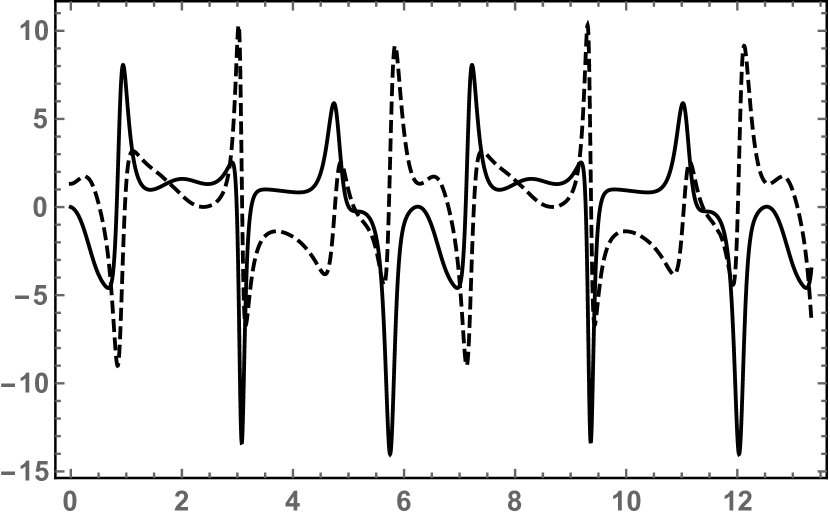
Figure 43: Initial value problem (19), (20). Graphs of the real (bold curve) and imaginary (dashed curve) parts of the coordinate $w_{3}(t)$.

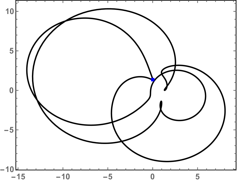
Figure 44: Initial value problem (19), (20). Trajectory, in the complex $z$-plane, of $w_{3}(t)$; period $4\pi$. The square indicates the initial condition $w_{3}(0)=1.32\mathbf{i}$.

Appendix C Mathematica Code

In this appendix, we provide the Mathematica 10 code that was used for producing the plots in Appendix B. Let us recall that these plots illustrate Examples 1 and 2 of Section 2.

See pages - of 427N2ExamplesArxiv_160118 See pages - of 427N3ExamplesArxiv_160118

References

• [1] F. Calogero, ”New solvable variants of the goldfish many-body problem”, Studies Appl. Math. (in press; published online 07.10.2015).
• [2] O. Bihun and F. Calogero, “A new solvable many-body problem of goldfish type”, J. Nonlinear Math. Phys. (in press). arXiv:13749 [math-ph].
• [3] F. Calogero, “A solvable N-body problem of goldfish type featuring $N^{2}$ arbitrary coupling constants”, J. Phys. A: Math. Theor. (submitted to, 18.09.2015).
• [4] O. Bihun and F. Calogero, “Generations of monic polynomials such that the coefficients of the polynomials of the next generation coincide with the zeros of a polynomial of the current generation, and new solvable many-body problems”, Lett. Math. Phys. (submitted to, 16.10.2015); arXiv: 1510.05017 [math-ph].
• [5] F. Calogero and D. Gómez-Ullate, Asymptotically isochronous systems, J. Nonlinear Math. Phys. 15, 410-426 (2008).
• [6] F. Calogero, Isochronous systems, Oxford University Press, Oxford, 2008 (264 pages); marginally updated paperback edition (2012).
• [7] F. Calogero, Classical many-body problems amenable to exact treatments, Lectures Notes in Physics Monographs m66, Springer, Berlin Heidelberg, 2001 (749 pages).
• [8] D. Gómez-Ullate and M. Sommacal, ”Periods of the goldfish many-body problem”, J. Nonlinear Math. Phys. 12, Suppl. 1, 351–362 (2005).