On the Asymmetric Longitudinal Oscillations of a Pikelner’s Model Prominence

Abstract

We present analytical and numerical models of a normal-polarity quiescent prominence that are based on the model of Pikelner (Solar Phys. 1971, 17, 44 ). We derive the general analytical expressions for the two-dimensional equilibrium plasma quantities such as the mass density and a gas pressure, and we specify magnetic-field components for the prominence, which corresponds to a dense and cold plasma residing in the dip of curved magnetic-field lines. With the adaptation of these expressions, we solve numerically the 2D, nonlinear, ideal MHD equations for a Pikelner’s model of a prominence that is initially perturbed by reducing the gas pressure at the dip of magnetic-field lines. Our findings reveal that as a result of pressure perturbations the prominence plasma starts evolving in time and this leads to the antisymmetric magnetoacoustic–gravity oscillations as well as to the mass-density growth at the magnetic dip, and the magnetic-field lines subside there. This growth depends on the depth of magnetic dip. For a shallower dip, less plasma is condensed and vice-versa. We conjecture that the observed long-period magnetoacoustic–gravity oscillations in various prominence systems are in general the consequence of the internal pressure perturbations of the plasma residing in equilibrium at the prominence dip.

————————————————————————————————

1 Introduction

Prominences are dense and cold solar coronal magnetic structures, which reveal high degree of complexity such as their long and thin threads (Tandeberg-Hansen, 1974). The average prominence temperature is about two hundred times lower and the mass density is approximately two hundred times higher than the ambient coronal values. Prominences are linked to the underlying photosphere by several foot-points and lie along the polarity inversion line. The length of prominences is within $50-500$ Mm, their height is $10-100$ Mm, and their average thickness is $15$ Mm (Priest, 1989).

Solar prominences can be classified into two groups: i) active prominences and ii) quiescent prominences (Zirin, 1988). Active prominences reveal life-times of no more than a few days, undergoing dramatic changes in plasma motions and magnetic activity. They are often associated with solar flares. Quiescent prominences can live for months, forming themselves over a magnetic neutral line that separates the regions of opposite magnetic polarities on the photosphere.

The first quiescent prominence models were devised about $60$ years ago (Menzel, 1951). Two classical models are commonly accepted, which are known as the Kippenhahn and Schlüter (1957), and Kuperus and Raadu (1974) models. In these models the cool and dense plasma is maintained against gravity by the magnetic tension at the local dip of the magnetic arcade. The distribution of magnetic polarity in this arcade prominence is the same as in the underlying photosphere, i.e. direct polarity. Kuperus and Raadu (1974) proposed a model in which the prominence, taking the form of a magnetic flux rope, is maintained in a vertical current-sheet with open magnetic-field lines. Below this current-sheet the X-point is present, and the prominence exhibits inverse polarity. Currently, there are two well-accepted 3D prominence models with inverse polarity: the sheared arcade and the flux-rope magnetic structures (Labrosse et al., 2010, and references cited therein).

While these classical models reveal the equilibrium magnetic configurations of quiescent prominences, a recent trend is emerging with the observational and theoretical reports that led to the foundation of plasma and wave dynamics within such stable magnetic configurations of the prominence system. (Luna and Karpen 2012; Luna, Díaz and Karpen 2012) have found that the observed large-amplitude longitudinal prominence oscillations ($>20$ km s^-1) are driven by the projected gravity along the flux tubes and are strongly influenced by the curvature of the dips of the magnetic field in which the prominence threads reside. These oscillations reported by both Luna and Karpen (2012) and Luna, Díaz and Karpen (2012) for slow magnetoacoustic–gravity modes, are the symmetric longitudinal oscillations. Terradas et al. (2013) have studied the excitation of fast as well as slow antisymmetric magnetoacoustic–gravity modes of a prominence; they also dealt with magnetoststatic (MHS) equilibrium and performed linear MHD normal mode analysis. Small-amplitude longitudinal (slow) and fast transverse prominence oscillations either as a collective motion or as an individual thread ($\approx 2-3$ km s^-1) are well observed and modeled in the solar atmosphere (Arregui, Oliver and Ballester, 2012, and references cited therein). Terradas, Oliver and Ballester (2001) have reported that slow magnetoacoustic–gravity longitudinal oscillations of the quiescent prominences can be damped by the radiation and Newtonian cooling. Longitudinal prominence oscillations were observed and modeled by Li and Zhang (2012), Zhang et al. (2012), Shen et al. (2014), Bi et al. (2014), and Chen, Harra and Fang (2014).

While a number of generalizations to the seminal models of Kippenhan and Schlüter (1957) and Kuperus and Raadu (1974) were constructed in the past, we propose an arcade model of normal polarity as sketched by Pikelner (1971). Pikelner (1971) only sketched the model but he did not support it by any analytical expression. Our aim is to devise an analytical arcade model of a prominence by presenting the stringent mathematical expressions for the equilibrium prominence quantities. Our devised analytical model of prominence is significant to the bounded prominence structures that exhibit collective wave motions as well as the plasma dynamics. Additionally, our goal is to implement this analytical model into the FLASH numerical code (Lee, 2013) and develop a numerical model. This numerical model allows us to study a number of plasma phenomena. As a particular application of this model, in the present paper, we simulate magnetoacoustic–gravity waves in the prominence that result from a localized pressure pulse. This is the first article describing in detail our newly developed analytical model and its one numerical experiment on long-period prominence oscillations to shed light on their driving physical mechanism. The derived results are applicable to understand the physical processes of the prominence during evolved non-linear oscillations and are thereby useful for prominence seismology and related observations.

This article is organized as follows: Section 2 describes the analytical model of a quiescent prominence that is based on Pikelner’s model. The results of numerical simulations are outlined in Secion 3. In the last section we present the discussion and conclusions.

2 Analytical Model of Quiescent Prominence

sec:ana_model

2.1 MHD equations

sec:equ_model We consider a gravitationally stratified and magnetically confined plasma, which is described by ideal two-dimensional (2D) magnetohydrodynamic (MHD) equations:

eq:MHD˙rho$${{\partial\varrho}\over{\partial t}}+\nabla\cdot(\varrho{\textbf{{V}}}) = 0\,,$$ (1)

eq:MHD˙V$$\varrho{{\partial{\textbf{{V}}}}\over{\partial t}}+\varrho\left({\textbf{{V}}}\cdot\nabla\right){\textbf{{V}}} = -\nabla p+\frac{1}{\mu}(\nabla\times{\textbf{{B}}})\times{\textbf{{B}}}+\varrho{\textbf{{g}}}\,,$$ (2)

eq:MHD˙B$${{\partial{\textbf{{B}}}}\over{\partial t}} = \nabla\times({\textbf{{V}}}\times{\textbf{{B}}})\,,$$ (3)

eq:MHD˙divB$$\nabla\cdot{\textbf{{B}}} = 0\,,$$ (4)

eq:MHD˙p$${\partial p\over\partial t}+{\textbf{{V}}}\cdot\nabla p = -\gamma p\nabla\cdot{\textbf{{V}}}\,,$$ (5)

eq:MHD˙CLAP$$p = \frac{k_{\rm B}}{m}\varrho T\,.$$ (6)

Here ${\varrho}$ is the mass density, $p$ a gas pressure, ${\textbf{{V}}}=[V_{x},V_{y},0]$, ${\textbf{{B}}}=[B_{x},B_{y},0]$, and ${\textbf{{g}}}=[0,-g,0]$ represent the plasma velocity, the magnetic field and gravitational acceleration, respectively. The value of $g$ is equal to $274$ m s^-2. In addition, $T$ is the plasma temperature, $\gamma=5/3$ is the adiabatic index, $\mu$ is the magnetic permeability of the plasma, and $m$ is a particle mass that is specified by mean molecular weight of $0.6$. Although this value is valid for fully ionized plasma of the corona we believe that its larger value will not qualitatively change the response of the system. We assumed that $z$ is an invariant coordinate ($\partial/\partial z=0$) and we set the $z$-components of velocity and magnetic field equal to zero. This assumption removes Alfvén waves from the system in which magnetoacoustic–gravity waves are able to propagate.

2.2 Equilibrium Configuration

sec:equil We assume that the solar atmosphere is in static equilibrium ${\textbf{{V}}}_{e}={\bf 0})$. It follows from Equations (eq:MHD_rho)–(eq:MHD_p) that in such model this equilibrium is described by

eq:st˙p$$-\nabla p_{\rm{e}}+\frac{1}{\mu}(\nabla\times{\textbf{{B}}}_{\rm{e}})\times{\textbf{{B}}}_{\rm{e}}+\varrho_{\rm{e}}{\textbf{{g}}}={\textbf{{0}}},$$ (7)

eq:st˙B$$\nabla\cdot{\textbf{{B}}}_{\rm{e}}=0.$$ (8)

Here the subscript _e corresponds to the equilibrium quantities.

As a result of Equation (eq:st_B), the magnetic field, ${\textbf{{B}}}_{\rm{e}}$, can be expressed with the use of the magnetic-flux function, $A(x,y)$, as

$${\textbf{{B}}}_{\rm e}(x,y)=\nabla\times\left(A\hat{\textbf{{z}}}\right)\ilabel{eq:Be}$$ (9)

with $\hat{\textbf{{z}}}$ being a unit vector along the $z$-direction. As a result, the $x$- and $y$-components of the magnetic field are

$$\ilabel{eq:BxBy}B_{\rm{ex}}=\frac{\partial A}{\partial y},\,\hskip 8.53581ptB_{\rm{ey}}=-\frac{\partial A}{\partial x}.$$ (10)

Under the above assumptions, Equations (eq:MHD_CLAP) and (eq:st_p) are reduced to the following expressions (Low, 1975, 1980):

eq:st˙px$$\nabla^{2}A(x,y) = -\mu\frac{\partial p_{\rm{e}}(A,y)}{\partial A},$$ (11)

eq:st˙py$$\varrho_{\rm{e}}(x,y)g = -\frac{\partial p_{\rm{e}}(A,y)}{\partial y}.$$ (12)

Now, we can specify the RHS of Equation (11) and thereafter proceed to solve this equation for the magnetic field, however, this is a formidable nonlinear Dirichlet problem to solve (Low, 1975, 1980). Here we adopt the approach proposed by (Low, 1980, 1981, 1982) who reversed the mathematical problem by specifying the magnetic field first and then deriving the equilibrium conditions for the mass density and the gas pressure. By defining the magnetic flux function, $A(x,y)$, we can in general integrate Equation (11) to find formula for the equilibrium gas pressure and then using Equation (eq:st_py) calculate the mass density. Following this idea, we integrate Equation (eq:st_px) regarding $y$-coordinate as a fixed parameter (Solov’ev, 2010). Then, a variation of $A$ is

$${\mathrm{d}}A=\frac{\partial A}{\partial x}{\mathrm{d}}x+\frac{\partial A}{\partial y}{\mathrm{d}}y+\frac{\partial A}{\partial z}{\mathrm{d}}z=\frac{\partial A}{\partial x}dx,$$ (13)

as a result of $\partial A/\partial z=0$ and ${\mathrm{d}}y=0$.

Using this expression in Equation (eq:st_px) we obtain

$$\mu p_{\rm{e}}=-\int\left(\frac{\partial^{2}A}{\partial x^{2}}+\frac{\partial^{2}A}{\partial y^{2}}\right)\frac{\partial A}{\partial x}{\mathrm{d}}x+\mu C(y),$$ (14)

where $C(y)$ is an integration function. As the integration over the first integrand can be performed explicitly, therefore, we obtain

$$\ilabel{eq:pe1}\mu p_{\rm{e}}=-\frac{1}{2}\left(\frac{\partial A}{\partial x}\right)^{2}-\int\frac{\partial^{2}A}{\partial y^{2}}\frac{\partial A}{\partial x}{\mathrm{d}}x+\mu C(y).$$ (15)

Figure 1.: Vertical hydrostatic temperature profile from Avrett and Loeser (2008).fig:h˙stat˙temp

As the magnetic field tends to zero at $x\to\pm\infty$ and $p_{\rm e}=p_{\rm h}(y)$ we find

$$C(y)=p_{\rm{h}}(y),$$ (16)

where $p_{\rm{h}}(y)$ is the hydrostatic pressure of the magnetic-free solar atmosphere with

$$-\frac{\partial p_{\rm{h}}}{\partial y}=\varrho_{\rm{h}}(y)g,$$ (17)

which is specified by a temperature profile $T_{\rm e}(y)$. In this case we adopt the temperature model of Avrett and Loeser (2008). Note that temperature reaches its minimum of 4300 K at $approx0.6$ Mm (Figure fig:h_stat_temp). At higher altitudes, the temperature rises with $y$. At the transition region that is located at $y\approx 2.1$ Mm, the temperature shows abrupt growth of about 0.8 MK in the solar corona at $y=10$ Mm. The temperature profile determines uniquely the hydrostatic mass density and a gas pressure, which fall off with $y$ (not shown here). For a recent implementation of $p_{\rm h}(y)$ see Murawski et al. (2013). From Equation (eq:pe1) we get

$$\ilabel{eq:pe}p_{\rm{e}}(x,y)=p_{\rm{h}}(y)-\frac{1}{\mu}\left(\int\frac{\partial^{2}\!A}{\partial y^{2}}\frac{\partial A}{\partial x}{\mathrm{d}}x+\frac{1}{2}\left(\frac{\partial A}{\partial x}\right)^{\!2}\right).$$ (18)

From Equation (eq:st_py) it follows that in order to find the distribution of the mass density, $\varrho_{\rm e}(x,y)$, we need to calculate $\partial p_{\rm{e}}(A,y)/\partial y$. In order to execute this action, we perform the following analysis. Let $A(x,y)$ be a function of independent variables, $(x,y)$. Then we can express any differentiable function, $S(x,y)$, as $S(y,A(x,y))$ and the following equation is derived:

eq:dSdy$$\frac{\partial S(x,y)}{\partial y}=\frac{\partial S(y,A)}{\partial y}+\frac{\partial A}{\partial y}\frac{\partial S(y,A)}{\partial A}.$$ (19)

Then

$$\ilabel{eq:dSdy1}\frac{\partial S(y,A)}{\partial y}=\frac{\partial S(x,y)}{\partial y}-\frac{\partial A}{\partial y}\frac{\partial S(y,A)}{\partial A}.$$ (20)

Replacing $S(y,A)$ by $p_{\rm{e}}(y,A)$ and utilizing Equation (eq:st_px) we find

$$\ilabel{eq:dSdy2}\frac{\partial p_{\rm{e}}(y,A)}{\partial y}=\frac{\partial p_{\rm{e}}(x,y)}{\partial y}-\frac{\partial A}{\partial y}\nabla^{2}A,$$ (21)

and then expressing $p_{\rm{e}}(y,A)$ by Equation (eq:pe) we find the formula for the equilibrium mass density,

$$\ilabel{eq:rho}\varrho_{\rm{e}}(x,y)g=\varrho_{\rm{h}}(y)g+\frac{1}{\mu}\left[\frac{\partial}{\partial y}\left(\int\frac{\partial^{2}\!A}{\partial y^{2}}\frac{\partial A}{\partial x}{\mathrm{d}}x+\frac{1}{2}\left(\frac{\partial A}{\partial x}\right)^{\!2}\right)-\frac{\partial A}{\partial y}\nabla^{2}A\right].$$ (22)

Note that $p_{\rm{e}}$ and $\varrho_{\rm{e}}$ are specified by Equation (eq:pe) and Equation (eq:rho), respectively. These equations are general in nature. Specific forms of $p_{\rm e}$ and $\varrho_{\rm e}$ are obtained after the estimation of $A(x,y)$, which is a free function. This function must be chosen by some physical reasons. In the following part of this article we present this function for a solar prominence.

2.3 Pikelner’s Prominence Model

For the solar prominence model of Pikelner (1971) we adopt the following expression for the flux function:

$$\ilabel{eq:A_{P}ik}A(x,y)=\frac{B_{0}}{k}(1+a_{1}k^{2}x^{2})\exp[-k^{2}(a_{2}(y-y_{\rm ref})^{2}+x^{2})]\,,$$ (23)

where $a_{1}$ and $a_{2}$ are some positive constants, $k$ denotes inverse length, which determines the spatial scale of the structure, and $B_{0}$ is the magnetic-field strength at the reference point, ($x=0,y=y_{\rm ref}$). We choose and hold fixed $y_{\rm ref}=10\,{\rm Mm},\,k=1/50\,({\rm Mm})^{-1}$, and $B_{0}\approx 6\,{\rm Gauss}$. This choice of $A(x,y)$ leads to magnetic-field lines that are characteristic for a prominence and the equilibrium mass density and gas pressure can be given by relatively simple expressions.

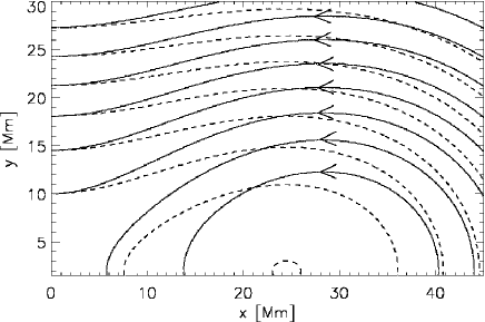
Figure 2.: Spatial profiles of magnetic-field lines in Pikelner’s prominence model for $a_{2}=1.5$, $a_{1}=1.6$ (dashed lines) and $a_{1}=2.0$ (solid lines). Note that only the right-hand ($x\geq 0$) side of the prominence is displayed.fig:mag

The magnetic field resulting from Equations (eq:A_Pik) and (eq:BxBy) is illustrated in Figure fig:mag. The dip in the magnetic-field vectors is discernible along the vertical line $x=0$, and this dip grows with $a_{1}$ as magnetic lines are more tilted for a large value of $a_{1}$ Figure fig:mag). Having specified $A(x,y)$ by Equation (eq:A_Pik), with the use of Equations (eq:pe) and (eq:rho), we express the equilibrium gas pressure and the mass density for the Pikelner’s model as

eq:eq˙press$$p_{\rm e}(x,y)=p_{\rm h}(y)-$$ (24)

$$\mbox{}-0.5\,[(p_{3}x^{4}+p_{4}x^{2}+p_{7})y^{2}+p_{9}x^{4}x^{2}+p_{1}x^{4}+p_{2}x^{2}-2a_{2}^{2}]\times$$

$$\times\exp[p_{10}(y-y_{\rm ref})^{2}+p_{11}x^{2}]B_{0},$$

eq:eq˙dens$$\varrho_{\rm e}(x,y)=\varrho_{\rm h}(y)+$$ (25)

$$\mbox{}+4\,(p_{5}x^{4}+p_{6}x^{2}+p_{8})(y-y_{\rm ref})\exp[p_{10}(y-y_{\rm ref})^{2}+p_{11}x^{2}]B_{0}/g,$$

where

$$p_{1}=k^{4}(-2a_{1}^{2}a_{2}-8a_{1}^{2}+8a_{1}), p_{2}=k^{2}(-4a_{1}a_{2}+4a_{1}^{2}-8a_{1}+4),$$

$$p_{3}=4k^{6}a_{1}^{2}a_{2}^{2}, p_{4}=8k^{4}a_{1}a_{2}^{2},$$

$$p_{5}=k^{6}(a_{1}^{2}a_{2}^{2}-a_{1}^{2}a_{2}), p_{6}=k^{4}[2a_{1}a_{2}^{2}+(-a_{1}^{2}-2a_{1})a_{2}],$$

$$p_{7}=4k^{2}a_{2}^{2}, p_{8}=k^{2}[a_{2}^{2}+(a_{1}-1)a_{2}],$$

$$p_{9}=4k^{6}a_{1}^{2}, p_{10}=-2k^{2}a_{2},\;p_{11}=-2k^{2}.$$

The prominence equilibrium mass density and temperature profiles that result from Equations (eq:eq_press), (eq:eq_dens), and (eq:MHD_CLAP) are displayed in Figure fig:density. Note that the prominence plasma occupies the dense (at $x=0$, $y\approx 20$ Mm) and cold (at $y\approx 35$ Mm) region. While the classical models of a prominence exhibit a single cold region that is centrally located, Pikelner’s model reveals the central cold region and two side, cold regions (Figure fig:density c and d). These side regions result from faster fall-off in gas pressure than in mass density.

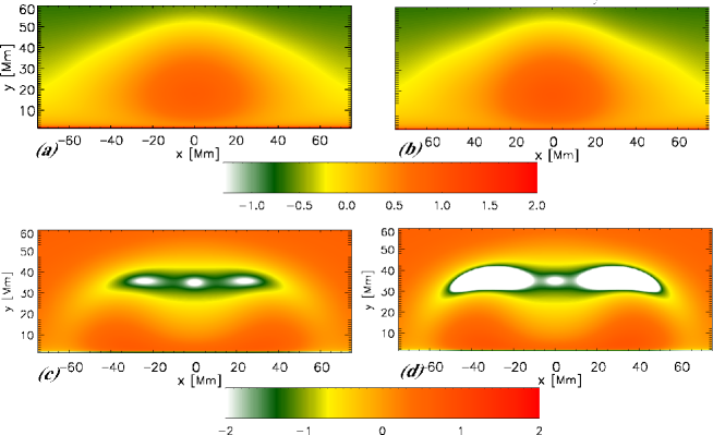
Figure 3.: Spatial profiles of $\log(\varrho_{\rm e}(x,y))$ for $a_{2}=1.5$, $a_{1}=1.6$ (a) and $a_{1}=2.0$ (b). Temperature profiles $\log(T_{\rm e}(x,y))$ for $a_{1}=1.6$ (c) and $a_{1}=2.0$ (d).fig:density

3 Results of Numerical Simulations

sect:num_res

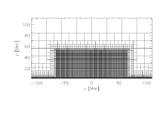
Figure 4.: Block system used in the simulation studies.fig:blocks

Equations (eq:MHD_rho) – (eq:MHD_CLAP) are solved numerically using the FLASH code (Lee and Deane, 2009; Lee, 2013). This code implements a third-order, unsplit Godunov solver with various slope limiters and Riemann solvers (e.g. Tóth, 2000), as well as adaptive mesh refinement (MacNeice et al., 1999). We use the minmod slope limiter and the Roe Riemann solver. For all cases considered we set the simulation box as $(-110,110)\,{\rm Mm}\times(1,111)\,{\rm Mm}$ and impose boundary conditions by fixing in time all plasma quantities at all four boundaries to their equilibrium values. In all of our studies we use a static grid with a minimum (maximum) level of refinement set to 3 (9). The whole computational region is covered by a set of blocks with different grid cell sizes, which are organized in a hierarchical fashion using a tree data structure Figure (fig:blocks). The blocks at the first/top level of the tree consist of the largest cells, while their children have a factor of two smaller cells and are called to be refined. As a result, at level $3$ ($9$) the block size contains cells by the factor of $2^{2}$ ($2^{8}$) smaller than the top level cells. In this way, we attain the effective finest spatial resolution of about $20$ km below the transition region, $y=2.1$ Mm. The total number of grid cells implemented at $t=0$ seconds in the model is almost $10^{6}$. The typical computation time is 48 hours and the computations were performed with the $32$ CPUs.

3.1 Perturbations in the Pikelner’s Prominence

We initially perturb the above described equilibrium impulsively by adding a Gaussian pulse in a gas pressure, viz

$$\ilabel{eq:perturb}p(x,y,t=0)=p_{\rm e}(x,y)\left[1+A_{\rm p}\exp\left(-\frac{x^{2}+(y-y_{\rm 0})^{2}}{w^{2}}\right)\right]\,.$$ (26)

Here the symbol $A_{\rm p}$ denotes the amplitude of the initial pulse, $y_{\rm 0}$ its initial position, and $w$ is its width. The relative amplitude of the initial pressure pulse, i.e., $A_{\rm p}=-0.95$ means that we consider large-amplitude oscillations. We set and hold fixed $A_{\rm p}=-0.95\,$, $w=4$ Mm, and $y_{\rm 0}=35$ Mm, where $y_{\rm 0}$ corresponds to the position of bottom of the magnetic dip. The negative value of $A_{\rm p}$ mimics rapid cooling of plasma, which was recently studied by Murawski, Zaqarashvili and Nakariakov (2011). The sudden, spatially localized decrease in the gas pressure around the null point sucks the plasma in, creating a region of the density enhancement around the $X$-point. The compression of mass density is subject to buoyancy force, and its influence is expressed by changing the blob shape.

3.2 Dynamics of the Perturbed Plasma

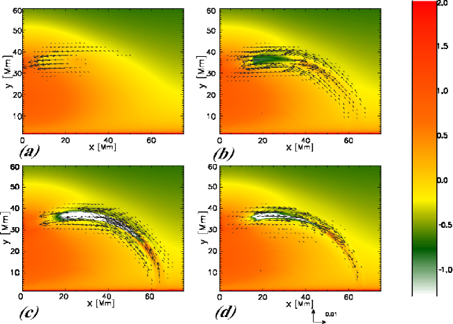
Figure 5.: Spatial profiles of $\log(\varrho(x,y))$ for $a_{1}=1.6$ and $a_{2}=1.5$ at $t=1000$ seconds (a), $t=2500$ seconds (b), $t=4000$ seconds (c), and $t=5500$ seconds (d). The vectors denote the velocity of the perturbed plasma. The only $x\geq 0$ Mm is displayed.fig:dens-time-6

Figure 6.: The relative mass of the prominence vs. timefig:mass

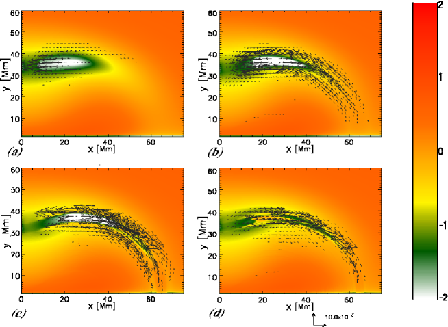
Figure 7.: Spatial profiles of $\log(T(x,y))$ for $a_{1}=1.6$ and $a_{2}=1.5$ at $t=1000$ seconds (a), $t=2500$ seconds (b), $t=4000$ seconds (c), and $t=5500$ seconds (d). The velocity vectors are denoted by arrows.fig:temp-time-6

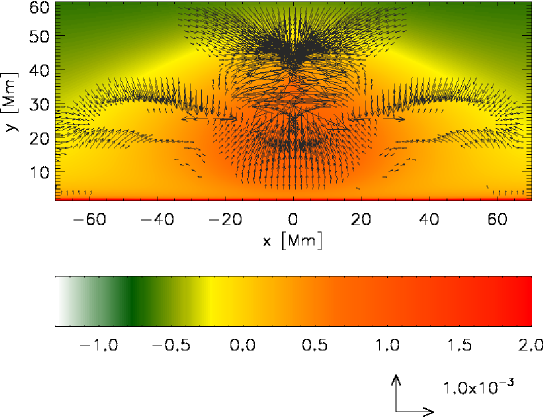
Figure 8.: Spatial profiles of $\log(\varrho(x,y))$ for $a_{1}=1.6$ at $t=250$ seconds. The vectors denote the velocity of the perturbed plasma. fig:rhoVxVy

Figure 9.: Time-signatures of $\varrho(x=0\,{\rm Mm},y=35\,{\rm Mm})$ vs. time for $a_{1}=1.6$ (dashed line) and $a_{1}=2.0$ (solid line).fig:dens-time-a1

Figure 10.: Time-signatures of velocity $V_{x}(x=20\,{\rm Mm},y=35\,{\rm Mm})\,{\rm km\,s^{-1}}$ (the left panel) and $V_{y}(x=20\,{\rm Mm},y=35\,{\rm Mm})\,{\rm km\,s^{-1}}$ (the right panel) vs time for $a_{1}=2.0$. fig:VxVy

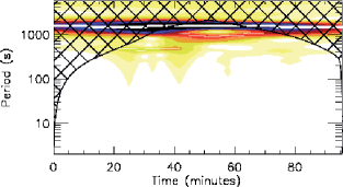
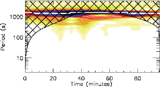
Figure 11.: The wavelet spectrum of velocity $V_{x}(x=20\,{\rm Mm},y=35\,{\rm Mm})\,{\rm km\,s^{-1}}$ (the left panel) and $V_{y}(x=20\,{\rm Mm},y=35\,{\rm Mm})\,{\rm km\,s^{-1}}$ (the right panel) for $a_{1}=2.0$. fig:WLT˙VxVy

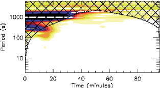
Figure 12.: The Fast Fourier Transform (FFT) spectrum of time-signatures of mass density (the left panel) and the wavelet analysis of the density (the right panel) for $a_{1}=2.0$ . fig:period˙rho

Figure 13.: Maximum of the mass density taken from the left panel of Figure fig:dens-time-a1 vs. $a_{\rm 1}$.fig:rhomax

Figure fig:dens-time-6 displays $\log(\varrho_{\rm e}(x,y,t))$ at four consecutive moments of time. As a result of the initial perturbation magnetoacoustic–gravity waves, which propagate in the system are essentially excited within the Pikelner’s prominence. However, these waves quickly leave the prominence domain. Later the under-pressure that settles at the launching place results in slow magnetoacoustic–gravity waves, which propagate essentially along the magnetic-field lines (Figure fig:dens-time-6 b). This under-pressure region brought some extra plasma from the ambient region into the launching place (Figure fig:dens-time-6 c and d).

Figure fig:mass illustrates the relative mass, $M_{\rm r}$, of the prominence. This mass is evaluated within the region $|x|\leq 20$ Mm, 20 Mm $\leq y\leq$ 45 Mm. Indeed, according to our expectations, this mass grows in time; at $t=0$ s, $M_{\rm r}=1$ while at $t=4000$ s, $M_{\rm r}$ reaches a magnitude of 1.13.

Figure fig:temp-time-6 shows temperature profiles at four instants of time. We see that plasma at the top of the Pikelner’s arcade becomes colder than in the ambient medium. As we are considering adiabatic equations, the cooling plasma results from the inflow of plasma, which is caused by the initial depression in the gas pressure there. As a result of this depression plasma is attracted by the pressure gradient force into the launching place.

Note that we do not include any dissipation mechanism in our model, such as radiation or thermal conduction. The initial negative pressure imbalance produces an increase of the mass density at the dip of the model prominence because it produces an inflow there mainly from chromospheric plasma, which is seen in Figure fig:rhoVxVy after the first 250 seconds of the simulation. As the dip is a potential well, some part of the inflowing plasma is trapped there and the mass density grows there. A similar physical explanation can be applied to the temperature field of the prominence. The plasma flows from the foot-points of the prominence along its field lines, which is colder than the plasma in the dip at $t=0$ seconds.

Figure fig:dens-time-a1 displays the temporal signatures that are drawn by collecting wave signals in the mass density at the point $(x=0,y=35)$ Mm, which corresponds to the location of the prominence dip. These time-signatures reveal an initial phase with strong mass-density variations. These initial phase lasts until $t\approx 1500$ seconds. Later on, the oscillations are of lower amplitude indicating a strong attenuation. The attenuation may result from energy leakage through the foot-points of the prominence that are located at the transition region, and also from the dip in magnetic-field lines. We will discuss some estimations to support the inherent wave-leakage process to dissipate the magnetoacoustic oscillations in the later part of the manuscript. The temporal evolution of the mass density exhibits a clear non-linear behavior because the initial mass density, i.e. the equilibrium value, is smaller than the ending value, which remains almost constant. The velocity field also oscillates according to the mass-density perturbations.

Figure fig:VxVy shows the velocity oscillation near the maximum of the prominence at ($x=20,\,y=35$) Mm. The velocity-field perturbations are aligned with the magnetic-field lines indicating that the motions are associated with slow modes.

These oscillations for the case of $a_{1}=2.0$, which represent the slow magnetoacoustic–gravity oscillations along the arcade, are analyzed by the Fast Fourier Transform (FFT) method. They exhibit the main period of $1577$ seconds as is seen in Figure fig:WLT_VxVy and fig:period_rho.

Figure fig:rhomax shows that the maximum of the mass density, $\varrho_{\rm max}$, grows with $a_{\rm 1}$. Note that a larger value of $a_{\rm 1}$ corresponds to a larger depth of the dips in the magnetic-field lines; the prominence with a larger depth of the dips, once perturbed and departed from the equilibrium, exhibits a larger amplitude of the slow magnetoacoustic–gravity oscillations. As a result, more plasma can be trapped in the dips and the mass density becomes larger there, which explains the growing trend exhibited in Figure fig:rhomax.

Figure 14.: Variation of attenuation time $\tau$ vs. $a_{1}$.fig:tau

From Figure fig:dens-time-a1 we infer that a larger depth of the dips in the magnetic-field lines of a prominence leads to more oscillations in the mass density. Compare the solid line drawn for the larger depth in the dip with the dashed line, which corresponds to the case of the shallower dip.

The decay of the slow magnetoacoustic–gravity oscillations clearly decreases with the depth of the magnetic dip of a prominence. Figure fig:dens-time-a1 shows the fast attenuation and almost no oscillatory motion in the case of a shallower depth of the magnetic dip (dashed line). Figure fig:tau illustrates how attenuation time, $\tau$, grows with $a_{1}$. This means that a prominence with a larger dip (larger $a_{1}$) has a longer attenuation time (i.e., longer decay) and vice-versa.

Terradas et al. (2013) also found the larger oscillation wave periods for heavy prominences, while lower periods waves for light prominences.

Our model deals with the prominence and its ambient medium within the framework of the analytical technique of Solov’ev (2010) in which all forces acting on the plasma are taken into account. The oscillations excited in the system are not pure gravity or gas pressure, which is a different aspect compared to the previous model. The results in our article are associated with the antisymmetric longitudinal oscillations, which is a case study of our developed prominence model, and they match the results obtained by Terradas et al. (2013). However, it should be noted that the present model is based on nonlinear full MHD, while the model by Terradas et al. (2013) deals with magnetoststatic equilibrium and linear MHD normal-mode analysis. Therefore, in the context of the model description, these two cases have weak relevance. As stated above, the most likely dissipation mechanism of the excited oscillations is a wave leakage. This can result from energy leakage through the foot-points of the prominence, which are located at the transition region and from the energy leakage through the dip in magnetic-field lines also. Figure fig:energy shows the ratio of kinetic energy of the plasma just under the foot-points to the total kinetic energy above the foot-points, i.e., above the transition region. We see that this ratio grows with time, which indicates the leakage of energy from the prominence. Also in Figure fig:tot_vel, we see some leakage of energy under and above the prominence in the form of side streams of fast-moving plasma. Therefore, we quantify the presence of wave-leakage process as the dissipative agent for the evolved antisymmetric magnetoacoustic–gravity oscillations in Pikelner’s model prominence.

We infer from Figure fig:tot_vel that maximal pulse velocity is about $50$ km s^-1. This magnitude of the flow matches the typical observational data. For a large amplitude of the initial pulse, nonlinear effects would become more important. However, we have verified by running the appropriate cases that the general scenario of the system evolution remains similar.

Figure 15.: The ratio of energy under the foot-points to total energy.fig:energy

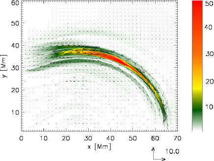
Figure 16.: Total velocity in km s^-1 (colour maps and vectors) for $a_{1}=1.6$ at time $t=6000$ seconds.fig:tot˙vel

4 Summary

In this article we adopted the analytical methods of Solov’ev (2010) to derive Pikelner’s model (Pikelner, 1971) of the normal polarity solar prominence. We implemented our analytical model into the publicly available FLASH code (Lee and Deane, 2009) and demonstrated the feasibility of fluid simulations in obtaining quantitative features in weakly magnetized and gravitationally stratified prominence plasma. In particular, we focused on perturbation of the developed normal polarity prominence model and its subsequent evolution. This perturbation was materialized by launching the initial pulse in gas pressure, which excited fast and slow magnetoacoustic–gravity waves. Fast waves were present at the initial stage of the prominence evolution while slow waves resulted later on and they lead to accumulation of plasma at the launching place which correspond to location of the magnetic dip. The parametric studies that we performed revealed that this accumulation varies with the shallowness of the dip; for a shallower dip there is less accumulated plasma and smaller oscillations at the magnetic dip.

Such large-amplitude oscillations consist of the motions with the observed velocities greater than $20$ km s^-1 (Arregui, Oliver and Ballester, 2012), which is also evident in our model results. Large-amplitude longitudinal oscillations can be excited by impulsive events, e.g., microflares due to impulsive heating (e.g., Zhang et al., 2012). Therefore in our model, we consider the gas pressure perturbation as a physical initial trigger mechanism of the oscillations that excite longitudinal fast and slow magnetoacoustic–gravity waves.

Our new analytical prominence model with realistic temperature distribution shows reasonable physical behavior of the typical slow acoustic oscillations in such quiescent prominences, which also matches the numerical results of Terredas et al. (2013). However, it should be noted that Terradas et al. (2013) deal with magnetoststatic (MHS) equilibrium and linear MHD normal mode analysis, while our model is based on non-linear full MHD equations. The general damping mechanism may most likely be the radiative cooling as invoked by many analytical and numerical investigations (e.g., Terradas, Oliver and Ballester, 2001; Terradas et al., 2013) related to the slow acoustic oscillations of the quiescent prominences. It should be noted that the fast dissipation of large-amplitude prominence oscillations is clearly evident in the observational data (e.g., Terradas et al. 2002; Arregui, Oliver and Ballester, 2012, and references cited therein). In the present case, we specifically found and quantified that the wave-leakage process is the dissipative agent for the antisymmetric magnetoacoustic–gravity oscillations in Pikelner’s model prominence. Since in our model we do not invoke any non-adiabatic thermodynamical effects, e.g., radiative cooling, for the dissipation of such oscillations, even then the wave-leakage turns out to be a very effective mechanism for the dissipation of asymmetric oscillations. The study of the relative significance of various dissipative agents on the magnetoacoustic–gravity mode oscillations, e.g., wave-leakage, radiative cooling, etc. may be an important task that we will study in a future project.

In conclusion, we have tested our new analytical prominence model numerically, and excited the slow magnetoacoustic–gravity oscillations along its magnetic dip by perturbing a gas pressure within the prominence. Our model will be further used in a more detailed study of prominence dynamics and to constrain its oscillations to exploit prominence seismology in order to deduce local plasma conditions.

Acknowledgements       This work was supported by the project from the Polish National Foundation (NCN) Grant no. 2014/15/B/ST9/00106. The work has also been supported by a Marie Curie International Research Staff Exchange Scheme Fellowship within the 7th European Community Framework Program (K. Murawski, A. Solov’ev and J. Kraśkiewicz.). In addition, A. Solov’ev thanks the Russian Scientific Foundation for the support in the frame of project No 15-12-20001 . The software used in this work was in part developed by the DOE-supported ASCI/Alliance Center for Astrophysical Thermonuclear Flashes at the University of Chicago. The visualizations of the simulation variables have been carried out using the IDL (Interactive Data Language) software package. Numerical simulations were performed on the Solaris cluster at Institute of Mathematics of M. Curie-Skłodowska University in Lublin, Poland.

References

- Arregui, Oliver and Ballester (2012) Arregui, I., Oliver, R., Ballester, J.L.: 2012, Living Rev. Solar Phys. 9, 2. DOI:10.12942/lrsp-2012-2
- Avrett and Loeser (2008) Avrett, E.H., Loeser, R.: 2008, Astrophys. J. Suppl. Sec. 175, 229. DOI:10.1086/523671
- Bi et al. (2014) Bi, Y., Jiang Y., Yang J., Hong J., Li H., Yang D., Yang B.: 2014, Astrophys. J. 790, 100. DOI:http://dx.doi.org/10.1088/0004-637X/790/2/100
- Chen, Harra and Fang (2014) Chen, P.F., Harra L.K., Fang C.: 2014, Astrophys. J. 784, 50. DOI:10.1088/0004-637X/784/1/50
- Kuperus and Raadu (1974) Kuperus, M., Raadu, M.A.: 1974, Astron. Astrophys. 31, 189.
- Kippenhahn and Schlüter (1957) Kippenhahn, R., Schlüter, R.: 1957, Zaitsch. Astroph. 43, 36.
- Labrosse et al. (2010) Labrosse, N., Heinzel, P., Vial, J.C., Kucera, T., Parenti, S., Gunar, S., Schmieder, B., Kilper, G.: 2010, Space Sci. Rev. 151, 243. DOI:10.1007/s11214-010-9630-6
- Lee (2013) Lee, D.: 2013, J. Comp. Phys. 243, 269. DOI:10.1016/j.jcp.2013.02.049
- Lee and Deane (2009) Lee, D., Deane, A.E.: 2009, J. Comp. Phys. 228, 952. DOI:10.1016/j.jcp.2008.08.026
- Li and Zhang (2012) Li, T., Zhang, J. 2012.: Astrophys. J. Lett. 760 (1), L10.
- Low (1975) Low, B.C.: 1975, Astrophys. J. 197 251. DOI:10.1086/153508
- Low (1980) Low, B.C.: 1980, Solar Phys. 65, 147. DOI:10.1007/BF00151389
- Low (1981) Low, B.C.: 1981, Astrophys. J. 246, 538. DOI:10.1086/158954
- Low (1982) Low, B.C.: 1982, Solar Phys. 75, 119. DOI:10.1007/BF00153465
- Luna et al. (2012) Luna, M., Karpen, J.: 2012, Astrophys. J. Lett. 750, 1. DOI:10.1088/2041-8205/750/1/L1
- Luna et al. (2012) Luna, M., Díaz, A.J., Karpen, J.: 2012, Astrophys. J. 757, 98. DOI:10.1088/0004-637X/757/1/98
- MacNeice et al. (2000) MacNeice, P., Olson, K.M., Mobarry, C., de Fainchtein, R., Packer, C.: 2000, Comp. Phys. Comm. 126, 330.
- Murawski, Zaqarashvili and Nakariakov (2011) Murawski, K., Zaqarashvili, T.V., Nakariakov, V.M.: Astron. Astrophys. 2011 533, A18. DOI:10.1051/0004-6361/201116942
- Murawski et al. (2013) Murawski, K., Ballai, I., Srivastava, A.K., Lee, D.: 2013, Mont. Not. Roy. Astron. Soc. 436, 1268. DOI:10.1093/mnras/stt1653
- Pikelner (1971) Pikelner, S.B.: 1971, Solar Phys. 17 44. DOI:10.1007/BF00152860
- Priest (1989) Priest, E.R. (ed.): 1989, Dynamics and structure of quiescent solar prominences, Reidel, Dordrecht.
- Solov’ev (2010) Solov’ev, A.A.: 2010, Astron. Rep. 54, 86. DOI:10.1134/S1063772910010099
- (23) Shen, Y., Liu, Y.D., Chen, P.F., Ichimoto, K.: 2014 Astrophys. J. 795 (2), 130. DOI:10.1088/0004-637X/795/2/130
- Tandeberg-Hanssen (1974) Tandeberg-Hanssen, E.: 1974, Solar Prominences, Reidel, Dordrecht.
- Terradas, Oliver and Ballester (2001) Terradas, J., Oliver, R., Ballester, J.L.: 2001, Astron. Astrophys. 378, 635. DOI:10.1051/0004-6361:20011148
- Terradas et al. (2002) Terradas, J., Molowny-Horas, R., Wiehr, E., Balthasar, H., Oliver, R. and Ballester, J.L., 2002,Astron. Astrophys. 393, 637. DOI:10.1051/0004-6361:20020967
- Terradas et al. (2013) Terradas, J., Soler, R., Díaz, A.J., Oliver, R., Ballester, J.L.: 2013, Astrophys. J. 778, 49. DOI:10.1088/0004-637X/778/1/49
- Tóth (2000) Tóth, G.: 2000, J. Comp. Phys. 161, 605. DOI:10.1006/jcph.2000.6519
- Zhang et al. (2012) Zhang, Q.M., Chen, P.F.,Xia, C., Keppens, R.: 2012, Astron. Astrophys. 542, 52. DOI:10.1051/0004-6361/201218786
- Zirin (1988) Zirin, H.: 1988, Astrophysics of the Sun, Cambridge Univ. Press, Cambridge.