Solutions to the Problem of $k$-SAT/$k$-COL Phase Transition Location

Abstract

As general theories, currently there are concentration inequalities (of random walk) only for the cases of independence and martingale differences. In this paper, the concentration inequalities are extended to more general situations. In terms of the theory presented in the paper, the condition of independence is $\frac{\partial y}{\partial t}=$ constant and martingale difference’s is $\frac{\partial y}{\partial t}=0$. This paper relaxes these conditions to $\frac{\partial^{2}y}{\partial u_{i}\partial t}\leq L$; i.e. $\frac{\partial y}{\partial t}$ can vary. Further, the concentration inequalities are extended to branching random walk, the applications of which solve some long standing open problems, including the well known problems of K-SAT and K-COL phase transition locations, among others.

1 Introduction

Let $G_{N,M}$ be a graph of $N$ vertices with $M$ edges, $e_{1}e_{2}...e_{\!{}_{M}}$ where $e_{i}$ is $(x_{i},y_{i})$, a pair of vertices. Sparse graphs, where $M=O(N)$, are considered here. 3-coloring problem (3-COL) is to color the graph so that no two adjacent vertices are colored with the same color. Or alternatively, 3-coloring problem is to find a 3-value assignment so that

$$\bigwedge_{i=1}^{M}C_{i}=T~{}\mbox{(True)}$$ (1.1)

where

$$C_{i}=x_{i}\oplus y_{i}$$

called ”clause”, $x_{i}$ and $y_{i}$ are drawn randomly from the $n$ vertices. $\oplus$ is defined by, $x\oplus y=T$ iff $x\neq y$. If $K$ colors are allowed, (1.1) represents a problem of K-coloring. Further, if $C_{i}$ contains more than two variables, (1.1) is a hypergraph K-coloring problem. Similarly, K-SAT is to find a truth value (two-value) assignment to (1.1) where

$$C_{i}=(v_{1}^{(i)}\oplus v_{2}^{(i)}\oplus...v_{k}^{(i)})$$

$v_{1}^{(i)},v_{2}^{(i)},...v_{k}^{(i)}$ are drawn randomly from $\{\neg x_{1},x_{1},\neg x_{2},x_{2},...,\neg x_{N},x_{N}\}$ and $\oplus$ is defined by, $x\oplus y=T$ iff $x\lor y=T$.

If a formula (i.e. $\bigwedge_{i=1}^{M}C_{i}$) can be satisfied (i.e. $\bigwedge_{i=1}^{M}C_{i}=T$) by an assignment, the formula is said ”satisfiable” It has been conjectured that there exists a critical point $\alpha_{3}$ such that if $\frac{m}{N}<\alpha_{3}$ almost all formulae are satisfiable, if $\frac{m}{N}>\alpha_{3}$ almost all formulae are unsatisfiable. For $k\geq 3$, researchers focus on proving upper bound and lower bound and asymptotic threshold ([1], [2] and reference therein). K-SAT is modeled as spin-glass like system in statistics physics and analogous estimates of the thresholds are obtained, though it is not known how similar these models are to K-SAT, and how far they deviate from it. The goal of this paper is to derive rigorous results of the phase transition location of K-SAT/K-COL, for K=2, 3, 4, …

2 Methodology

Actually, traditional K-SAT/K-COL phase transition phenomenon is the ”tip of the iceberg”, where relation between probability of satisfiability and $m$ (or $m/N$), namely function $\mathbb{P}(r)$, is concerned. $\mathbb{P}(r)$ is virtually $\mathbb{P}(r,A)$. But the parameter of algorithm $A$ is always omitted since it is always a complete algorithm. We consider $\mathbb{P}(r,A)$. Specifically, $\mathbb{P}(r,x)$ is considered where $x=\frac{i}{N}$ and $i$ is the number of variables fixed (frozen) beforehand. In other words, it is partial solution space that is provided to algorithms for searching, where $x_{1}=1,x_{2}=1,\ldots x_{i}=1$ for SAT. In 3-SAT for example, phase transition begins at $\{x,z\}=\{0.145,3.183\}$ (where $x=\frac{i}{N},z=\frac{m}{N}$), and all the way through to the end point of $\{0,4.396\}$ which is the location of 3-SAT phase transition in the traditional sense.

Randomly drawing a satisfiable formula is a process of branching random walk (BRW). If $u_{i}$ is deterministic, as opposed to random, satisfiable formulae of length $m$ account for $\Pi_{1}^{m}(1-u_{i})^{3}$, with $m$ factors of $(2N)^{3}$ being omitted. In this case, method of differential equation can be used to solve $u_{i}$. To show the required random parameters in a process of random graph evolution are ”deterministic” is the task of so called Differential Equation Method (DEM).

However, so far there has been no theoretical foundation for this method (DEM). The existing concentration inequalities or large deviation theory are not applicable to processes of random graph evolution which are branching random walk. We need a new theory, concentration inequality in branching random walk. This is the second contribution of this paper, which may be of independent interest.

3 Branching random walk vs. random walk

Let $(S_{n})_{i=1,2,...}$ be a real-valued random process, one-dimensional random walk, $S_{n}=X_{1}+X_{2}+...+X_{n}$; $X_{i}=S_{i}-S_{i-1}$. In the following, we give a BRW version of Chernoff bound for warming up,

$$Pr(|Q_{n}(\alpha)-na|\geq\lambda)\leq 2e^{-\frac{1}{2}c\lambda^{2}/n}$$

where $Q_{n}(\alpha)$ is $\alpha$ quantile and $\alpha\in[e^{-\frac{1}{2}c\lambda^{2}/n},1-e^{-\frac{1}{2}c\lambda^{2}/n}]$. Throughout, generation index $n$ will be omitted when no confusion can arise.

Unlike traditional view, here BRW is simply described by $<m(u),p(x)>$ where $m(u)$ is the expectation of offsprings (branching factor) of a parent at position $u$ and $p(x)$ is the children’s displacement (relative to their parent’s position) p.d.f, the probability (or proportion) density function, or mass probability if in discrete cases.

We refer a realization of BRW as a tree. Let $z^{(n)}_{1},z^{(n)}_{2},...$ be an enumeration of the positions of the particles (leaves) in the $nth$ generation and $Z^{(n)}$ its population; i.e. $Z^{(n)}=|\{z^{(n)}_{1},z^{(n)}_{2},...\}|$. There should appear an index on each tree in the notation which we omit. Let $u_{i}$ denote $x_{1}+x_{2}+...+x_{i}$, where $x_{i}$ is children’s displacement at generation $i$. The p.d.f of $(x_{1},x_{2},...,x_{n})$ is

$$\frac{\prod_{i=1}^{n}p_{i}(x_{i})m_{i}(u_{i})}{\sum_{x_{1},...x_{n}}\prod_{i=1}^{n}p_{i}(x_{i})m_{i}(u_{i})}$$

or

$$\frac{\prod_{i=1}^{n}p_{i}(x_{i})m_{i}(u_{i})dx_{1}dx_{2}...dx_{n}}{\int\prod_{i=1}^{n}p_{i}(x_{i})m_{i}(u_{i})dx_{1}dx_{2}...dx_{n}}$$ (3.1)

which gives the proportion density of $(x_{1},x_{2},...,x_{n})$ in the whole forest.

Theorem 3.1.

For BRW of independent branching (i.e. birth rate is independent of birthplace),

$$Pr(|Q_{n}(\alpha)-na|\geq\lambda)\leq 2e^{-\frac{1}{2}c\lambda^{2}/n}$$

Proof.

(In the full paper) ∎

4 An extension of concentration inequalities

So far concentration inequalities (of random walk) have not been extended enough for our purpose; we need concentration inequalities for the case of sum $S_{n}=X_{1}+X_{2}+...X_{n}$ where $X_{i}$ is neither bounded nor martingale differences. Let’s first introduce a simple and elegant inequality due to [3] and [4]. Given here is the version from [4] which improves [3].

Lemma 4.1.

If $E(X)=0$, then for all $\delta>0$ and $|t|/\delta\in[0,1]$

$$E(e^{tX})\leq 1+(t/\delta)^{2}E(e^{\delta|X|})\leq e^{(t/\delta)^{2}E(e^{\delta|X|})}$$

In particular, $E(e^{tX})\leq e^{t^{2}E(e^{|X|})}$, when $\delta=1$

Proof.

(In the full paper) ∎

Theorem 4.1.

(Azuma’s Inequality) (In the full paper)

We now show what else can make the concentration inequality hold, other than independence and martingale difference.

Let $E_{i-1}$ abbreviate $E(\cdot~{}|u_{i-1})$ where $u_{i-1}=(X_{1}+X_{2}+...+X_{i}-1)/N$. Note, for different purposes, we sometimes use $Y_{i}$, sometimes $S_{i}$ and sometimes $u_{i}$; they are the same thing but lower case $u_{i}$ refers to scaled variable. Define Doob’s (or McDiarmid’s) martingale

$$d_{i} =E_{i}(X_{i}+...+X_{n})-E_{i-1}(X_{i}+...+X_{n})$$

So

$$S_{n}-ES_{n}=\sum_{i=1}^{n}d_{i}$$

$$d_{i} =E_{i}(X_{i})-E_{i-1}(X_{i})+\sum_{l>i}(E_{i}(X_{l})-E_{i-1}(X_{l}))$$

$$=X_{i}-E_{i-1}(X_{i})+\sum_{l>i}(E_{i}(X_{l})-E_{i-1}(X_{l}))$$

It is easy to check that $E_{i-1}(d_{i})=0$.

Given $u_{i-1}$, $E_{i}(X_{l})$ is a function of $X_{i}$. $E_{i-1}(X_{l})=E_{X_{i}}\{E_{i}(X_{l})\}$ where $E_{X_{i}}(\cdot)$ takes expectation with respect to $X_{i}$.

Lemma 4.2.

If $|E_{i}(X_{l})-E_{i-1}(X_{l}|X_{i}=0)|\leq L\frac{|X_{i}|}{N}$ for $i<l$, then

$$|E_{i}(X_{l})-E_{i-1}(X_{l})|\leq L\frac{|X_{i}|}{N}+L\frac{E_{i-1}|X_{i}|}{N}$$ (4.1)

Proof.

(In the full paper) ∎

Lemma 4.3.

Let $A$ denote $1+L\frac{M}{N}$. If

$$|E_{i}(X_{l})-E_{i-1}(X_{l}|X_{i}=0)|\leq L\frac{|X_{i}|}{N}$$ (4.2)

for $i<l$, and $E(e^{\delta A|X_{i}|}\ |\ u_{i-1})\leq K$ (exponential moment existence) for a constant $\delta>0$ , $i=1,2,...$, then

$$Pr[|S_{n}-ES_{n}|\geq\lambda]\leq 2e^{-\frac{\delta^{2}}{4K^{2}}\frac{\lambda^{2}}{n}}$$ (4.3)

Obviously, Poisson distribution $Poisson(\lambda_{i})$ meets the exponential moment condition.

Proof.

(In the full paper) ∎

Corollary 4.2.

Lemma 4.3 holds if the condition (4.2) is replaced by

$$|E(X_{l}|u_{i})-E(X_{l}|u_{i}^{\prime})|\leq L|u_{i}-u_{i}^{\prime}|~{}~{}~{}~{}for~{}i<l\mbox{~{}~{}~{} (Lipschitz continuity) }$$ (4.4)

Proof.

By letting $u_{i}=\frac{1}{N}(X_{1}+...+X_{i-1}+X_{i})$ and $u_{i}^{\prime}=\frac{1}{N}(X_{1}+...+X_{i-1}+X_{i}^{\prime})$ where $X_{i}^{\prime}=0$, the conditions of Lemma 4.3 are met. ∎

The Lipschitz continuity condition of Corollary 4.2 is easily verifiable in practice, though it is a bit stronger than Lemma 4.3; e.g. in random graphs processes like K-COL, K-SAT, degree restricted graph process etc.

Remark. • In the case of independence, $E_{i}(X_{l})=E(X_{l})$ and thus $E_{i}(X_{l})-E_{i-1}(X_{l})$ = 0. In the case of martingale difference, $E_{i}(X_{l})$ is zero for $l>i$. In both,

$$\sum_{l>i}(E_{i}(X_{l})-E_{i-1}(X_{l}))=0$$

and $d_{i}$ is reduced to $X_{i}-E(X_{i})$ and $X_{i}$, respectively. In this case, condition of bounded difference, or finite exponential moment, a alone implies the concentration inequalities.

• It is easy to understand that the conditional expected increment of $Y_{t}$, $E(X_{t}|u_{i})$, can be written as $\partial y/\partial t$, where $y$ and $t$ are scaled variables. Then the condition above for the concentration inequalities can be rephrased as $\frac{\partial^{2}y}{\partial u_{i}\partial t}\leq L$. A very special case is $\frac{\partial^{2}y}{\partial u_{i}\partial t}=0$, the case of independence (where $\frac{\partial y}{\partial t}$ is constant) or martingale difference ($\frac{\partial y}{\partial t}=0$).

The following theorem provides easily verifiable conditions for concentration inequality in general cases where $\frac{\partial}{\partial u_{i}}(\frac{\partial y}{\partial t})\neq 0$; i.e. $\frac{\partial y}{\partial t}$ is not constant along the direction of increasing $u_{i}$.

Let $\lambda_{i}(u_{i})$ and $\nu_{i}(u_{i})$ denote $E(X_{i+1}|u_{i})$ and $E(X_{i+1}^{2}|u_{i})$ respectively; i.e. they are functions of $u_{i}$. Let $\lambda_{i}^{\prime}$ denote $\frac{d\lambda_{i}(u_{i})}{du_{i}}$, $\nu_{i}^{\prime}$ denote $\frac{d\nu_{i}(u_{i})}{du_{i}}$, $\lambda_{i}^{\prime\prime}$ the second order derivative and so on. We shall use term ”smooth function” to mean that the first several orders of derivatives exist.

Theorem 4.3.

If $E(e^{\delta A|X_{i}|}\ |\ u_{i-1})\leq K$ (existence of an exponential moment), then in the area where $\lambda_{i}$ and $\nu_{i}$ are smooth, the concentration inequality holds. In other words, there is equivalence between the smoothness of $\bar{u}$ and the concentration inequality.

Proof.

(In the full paper) ∎

We see from the above proof that Lipschitz continuity of $E(f(u_{n}))$ is ultimately down to the boundedness of derivatives of $f,\lambda,\nu$. So far we are only concerned with second derivatives for our purpose. To show the existence of higher derivatives of $E(f(u_{n}))$, we need to expand the function in higher Taylor order and then build recurrence relations the same way as above. The next section addressing BRW may need them for which we shall omit the proof.

5 Concentration inequalities in the context of BRW

We will use lowercase to denote scaled measure, and uppercase for non-scaled ones; for example, $Y_{i}=X_{1}+X_{2}+...+X_{i}$, $u_{i}=x_{1}+x_{2}+...+x_{i}$ where $x_{i}=X_{i}/N$. Unlike current BRW theory, in this paper distribution about (the number of) offspring is not needed and neither any assumption about the point process characterizing children motion. It is observed that any BRW can be formally described as

$$m_{i}(u_{i})p_{i}(X_{i})$$

where the branching factor $m_{i}$ dependents on the birthplace $u_{i}$, and

$$p_{i}(X_{i}):=p(X_{i}|u_{i-1})$$

is the probability density function, pdf, of children’s displacement which is dependent of the birthplace as well. Intuitively, if branching factor is smaller in farther area (from the mean path) than the nearer, the BRW should be more concentrative than without branching (or branching factor = 1). In other words, if you squeeze population towards its mean by reducing the birth rate in the remote area, then population distribution should be more concentrative. In terms of K-SAT, the instances with less-constraint have more descendants than those with more constraint; at least, the vice versa can not be true. Formally, let $Z(u_{i})$ is the total progeny of the particle at position $u_{i}$. Given $u_{i-1}$, this is a function of $X_{i}$, written as $Z(X_{i})$. Then we have

Assumption 1 (negative association).

$$Z(X_{i})\leq Z(X_{i}^{\prime})~{}\>\>\>\mbox{if}~{}\>|X_{i}|\geq|X_{i}^{\prime}|$$ (5.1)

This assumption implies also that, if $f(\cdot)$ is a monotonically increasing function, then

$$\int f(|X_{i}|)Z(X_{i})P(dX_{i})\leq\int f(|X_{i}|)P(dX_{i})\int Z(X_{i})P(dX_{i})$$ (5.2)

In BRW, a particle reproduces descendants generation by generation. The average $(\cdot)$ over the whole population is

$$\mathbb{E}^{\!{}^{(M)}}(\cdot)=\frac{\int(\cdot)m_{1}m_{2}...m_{\!{}_{M}}P(dX_{1}dX_{2}...dX_{\!{}_{M}})}{\int m_{1}m_{2}...m_{\!{}_{M}}P(dX_{1}dX_{2}...dX_{\!{}_{M}})}$$

where $m_{i}=m_{i}(u_{i-1}+X_{i}/N)$. This is dependent of the future generations, whereas in RW statistics is independent of future. Therefore any statistical measure in BRW is generation dependent.

Define

$$\mathbb{E}{\!{}^{(M)}}(\cdot\ |\ u_{i}):=\mathbb{E}_{i}^{\!{}^{(M)}}(\cdot)=\frac{\int(\cdot)m_{i+1}m_{i+2}...m_{\!{}_{k}}P(dX_{i+1}dX_{i+2}...dX_{\!{}_{M}})}{\int m_{i+1}m_{i+2}...m_{\!{}_{k}}P(dX_{i+1}dX_{i+2}...dX_{\!{}_{M}})}$$

By the law of iterated expectations

$$\mathbb{E}^{\!{}^{(M)}}(\cdot)=\mathbb{E}^{\!{}^{(M)}}(\mathbb{E}_{i}^{\!{}^{(M)}}(\cdot))$$

Define

$$\beta_{i}(u_{i}):=E~{}(m(u_{i}+X_{i+1}/N)\ |\ u_{i})$$

Define $\bar{S}_{n}$ := $E^{(M)}(S_{n})$. The following lemma is the counterpart of Lemma 4.3 in BRW. The proof is exactly the same as Lemma 4.3, which we omit.

Lemma 5.1.

Let $A$ denote $1+L\frac{M}{N}$. If (a) $E^{(M)}_{i-1}(e^{\delta A|X_{i}|})\leq K$ (exponential moment existence) for a constant $\delta>0$ , $i=1,2,...$, and (b)

$$|E^{(M)}_{i}(X_{l})-E^{(M)}_{i-1}(X_{l}|X_{i}=0)|\leq L\frac{|X_{i}|}{N}\mbox{ ~{} for $i<l$ }$$

then

$$Pr[\ |S_{n}-\bar{S}_{n}\ |\geq\lambda]\leq 2e^{-\frac{\delta^{2}}{4K^{2}}\frac{\lambda^{2}}{n}}\mbox{~{}~{} for $n\leq M$ }$$ (5.3)

The following theorem is the counterpart of Theorem 4.3, which gives easily verifiable conditions for BRW concentration inequality (5.3).

Theorem 5.1.

If $E(e^{\delta A|X_{i}|}\ |\ u_{i-1})\leq K$, then in the area where $\beta_{i}(u)$, $\lambda_{i}(u)$ and $\nu_{i}(u)$ are smooth, the concentration inequality holds.

Proof.

(In the full paper) ∎

Theorem 5.2.

Let $\Delta S_{i}$ denote $|S_{i}-\mathbb{E}S_{i}|$, $\epsilon$ be small compared with $\delta$, and $N^{1/2}\ll\lambda<\epsilon N$ ,

$$E\{e^{\delta|X_{i}|}\ |\ u_{i-1}\in(\bar{u}_{i-1}-\frac{\lambda}{N},\bar{u}_{i-1}+\frac{\lambda}{N})\}\leq K$$

Then

$$Pr \{\Delta S_{1}\leq\lambda~{}\land\Delta S_{2}\leq\lambda~{}\land\ldots\Delta S_{n}\leq\lambda\} \geq(1-2e^{-\frac{\lambda^{2}}{4cN}})^{n}$$ (5.4)

We call $(\bar{u}_{i-1}-\frac{\lambda}{N},\bar{u}_{i-1}+\frac{\lambda}{N})$ ”$\epsilon$ neighborhood”.

Proof.

(In the full paper) ∎

6 K-SAT phase transition

3-SAT. To start with, we are going to prove that proportion of frozen variables of satisfiable formulae is concentrating around their mean. Recall $z=\frac{m}{N}$ and $x=\frac{i}{N}$ so that the proportion of frozen variables $u=u(x,z)$. During the generation of satisfiable formulae, outliers are excluded accounting for only exponentially small amount. Up to $m-1$ for the kept formulae such a property holds that w.h.p. $u$ remains constant with only $\sim\frac{1}{N}$ of fluctuation if a clause of 3-SAT, 2-SAT or 1-SAT is removed or added. The property is referred as ”constant $u$”.

We only consider area far from singularities. Without confusing we denote $u_{m}$ by $u$ for K-SAT formulae of $m$-length (i.e. $m$ clauses). It is fact that fix one more variable, $x_{i+1}$, $u$ will be increasing, by the rate of $\frac{du}{dx}$. Since the frozen variables must be constant, either 0 or 1, the formula becomes one mixed with 2-SAT and 3-SAT clauses of all free variables; 2-SAT clause is due to one of its variable is set to 0. $\frac{du}{dx}$ is determined by how many new frozen variables are generated by fixing a free variable, to keep the formula satisfiable; the former is finite iff the later is finite. Let $N_{f}$ denote number of free variables and $m_{e}$ the number of 2-SAT clauses, i.e. those of the form $(x_{f}\vee y_{f})$.

A free variable $x_{f}$ has probability $p$ to be contained in a certain one of those $m_{e}$ 2-SAT clauses. The number of the 2-SAT clauses containing $x_{f}$ is written as $deg(x_{f})$ called $x_{f}$’s degree. Simple counting gives $p=\frac{2}{N_{f}}(1-\frac{1}{N_{f}})$ and the mean of $deg(x_{f})$ is $\theta=\frac{2m_{e}}{N_{f}}$. Those values are not important though. The important is that $x_{f}$’s degree is of $Poisson(\theta)$ distribution. It is easy to check that the 3-SAT (free) clauses contribute $O(\frac{1}{N})$ to $du/dx$, while behavior of CNF in singularity area (which we do not need to consider) could be extremal where 3-SAT free clauses may make significant contribution to $du/dx$. The same argument applies to $y_{f}$ whose degree has also $Poisson(\theta)$ distribution (difference of $O(\frac{1}{N})$ between $\theta$’s is neglected), and so on. Thus this branching process forms a Galton Watson tree rooted at $x_{f}$. The birth rate $\theta<1$ because $\frac{du}{dx}<\infty$. Denoting the number of $x_{f}$’s total progeny by $k_{x}$, we have $\mathbb{P}(k_{x}>k)\leq e^{-c\cdot k}$ for a positive $c$ (see, e.g, [7], and [8] for method). Hence constant $u$ and Theorem 5.2 hold for $m$.

Let $F\in A_{i}$ represent that $F$ is satisfiable in partial solution space of $x_{1}=1$, $x_{2}=1$, … ,$x_{i}=1$. It is easy to check that, for a formula of length $m$, $F_{m}$ with $u$, and a randomly drawn variable x from $\{x_{1},\neg x_{1},x_{2},\neg x_{2},...,x_{\!{}_{N}},\neg x_{\!{}_{N}}\}$ (note x is a 1-SAT clause)

$$1-u =\mathbb{P}(\mbox{x}F_{m}\in A_{i}\ |\ F_{m}\in A_{i})=\frac{i}{2N}+\mathbb{P}(x_{i+1}F_{m}\in A_{i}\ |\ F_{m}\in A_{i})\mbox{~{}~{}~{}(symmetry)}$$

$$=\frac{i}{2N}+\frac{\mathbb{P}(x_{i+1}F_{m}\in A_{i})}{\mathbb{P}(F_{m}\in A_{i})}=\frac{i}{2N}+\frac{\mathbb{P}(F_{m}\in A_{i+1})}{\mathbb{P}(F_{m}\in A_{i})}$$

Denoting $\mathbb{P}(F_{k}\in A_{i})$ by $P_{k}^{(i)}$ and noticing $P_{k}^{(i)}/P_{k-1}^{(i)}$ is $a(\frac{i}{N},\frac{k}{N})$ we have

$$\frac{P_{m}^{(i+1)}}{P_{m}^{(i)}} =\frac{P_{m}^{(i+1)}/P_{m-1}^{(i+1)}\cdot P_{m-1}^{(i+1)}/P_{m-2}^{(i+1)}\cdot P_{m-2}^{(i+1)}~{}...}{P_{m}^{(i)}/P_{m-1}^{(i)}\cdot P_{m-1}^{(i)}/P_{m-2}^{(i)}\cdot P_{m-2}^{(i)}~{}...}=\frac{\prod_{k=1}^{m}a(\frac{i+1}{N},\frac{k}{N})}{\prod_{k=1}^{m}a(\frac{i}{N},\frac{k}{N})}$$

$$=e^{\sum_{k=1}^{m}\ln\{a(\frac{i+1}{N},\frac{k}{N})-a(\frac{i}{N},\frac{k}{N})\}}$$

$$=e^{\int_{0}^{z}\frac{\partial\ln(a(x,t))}{\partial x}dt}$$

It follows that

$$1-u=\frac{x}{2}+e^{\int_{0}^{z}\frac{\partial\ln(a(x,t))}{\partial x}dt}$$

where $a(x,z)(=1-u^{3})$ is the branching factor. $\partial/\partial z$ of both sides of the above equation yields

$$(1-\frac{x}{2}-u)\frac{3u^{2}}{1-u^{3}}\frac{\partial u}{\partial x}-\frac{\partial u}{\partial z}=0$$ (6.1)

called 3-SAT PDE. With the initial condition $u=x/2$ when $z=0$, the solution of (6.1)

$$z=\frac{2(1-u^{3})}{3u^{2}}\ln\frac{1-u-\frac{x}{2}}{1-2u}$$

For K-SAT,

$$z=\frac{2(1-u^{K})}{Ku^{K-1}}\ln\frac{1-u-\frac{x}{2}}{1-2u}$$ (6.2)

The K-SAT PDE was first presented in [9] as conjecture.

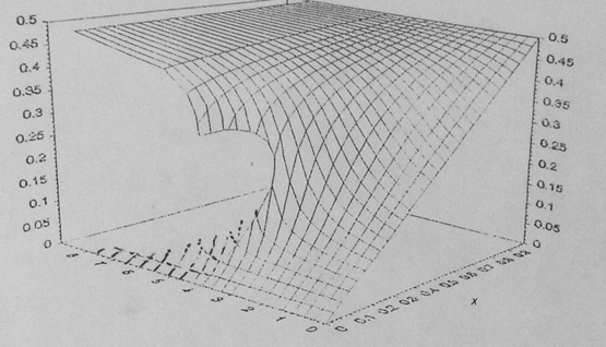
Figure 1: $u(x,z)$, 3-SAT

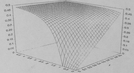
Figure 2: $u(x,z)$, 2-SAT

At the point $\{x_{0},z_{0}\}=\{0.145,3.183\}$, $u(x,z)$ starts to split into two surfaces, upper surface $S_{1}$ and lower surface $S_{2}$; in the area of $x<0.145$ and $z>3.183$, there are two solutions of $u$. $S_{1}$ and $S_{2}$ have overlap area, where $u_{\text{u}}(x,z)>u_{\text{l}}(x,z)$. $u_{\text{u}}(x,z)$ is on the upper surface and $u_{\text{l}}(x,z)$ on the lower surface.

BRW of satisfiable formula (denoted by ”SAT $F$”) generation can also go in $i$ direction, starting at $z=m/N$ and $x=1$ (i.e. $i=N$), reducing $i$ by 1 each step. In this direction, SAT $F$ increases (because $P_{m}^{(i-1)}=P_{m}^{(i)}\frac{1-x}{1-x/2-u}$ and $\frac{1-x}{1-x/2-u}>1$, by some calculation), while in $m$ direction SAT $F$ decreases because $1-u^{3}<1$. In fact, it can go in any direction; for example, decreasing $i$ and increasing $m$. Starting from $x=0.145,z=3.18$, there is a unique line in x-z plane corresponding to two routes of BRW, one in the upper surface and another in the lower surface, such that the number SAT $F$ of the upper surface is equal to the lower surface (so that probability of satisfiability is the same). That means along this line $u$ ”jumps”. The following is to find this critical line. Given that

$$P_{m+1}^{(i)}=(1-u^{3})P_{m}^{(i)}$$

and

$$P_{m}^{(i-1)}=P_{m}^{(i)}\frac{1-x}{1-x-(u-x/2)}=P_{m}^{(i)}\frac{1-x}{1-x/2-u}$$

Along the phase transition curve, it must be

$$\frac{(1-u_{u}^{3})^{dz}(\frac{1-x}{1-x/2-u_{u}})^{dx}}{(1-u_{l}^{3})^{dz}(\frac{1-x}{1-x/2-u_{l}})^{dx}}=1$$

Raising both sides of the above equation to power $\frac{1}{dx}$ yields

$$\frac{dz}{dx}=\frac{\ln(1-x/2-u_{u})-\ln(1-x/2-u_{l})}{\ln(1-u_{u}^{3})-\ln(1-u_{l}^{3})}$$

This is the threshold curve, at the end point of which (where $x=0$) $z$ is the traditional phase transition location $\alpha_{c}$. The following table lists some of the numerical results (bold numbers).

K :	3	4	5	6	7
best upper bound	4.51	10.23	21.33	43.51	87.88
$\boldsymbol{\alpha_{c}}$	4.396	10.077	21.234	43.45	87.84
spin glass model	4.267	9.931	21.117	43.37	87.79
best lower bound	3.52	7.91	18.79	40.62	84.82

7 K-COL phase transition

Similar to 3-SAT, let $F\in A_{i,j}$ represent that $F$ is satisfiable in partial solution space where $i$ variables (nodes) are frozen to 0, 1 and 2 respectively, and $j$ nodes which have satisfiable values at and only at {0, 1}, {0, 2} and {1, 2} respectively. Let $x=\frac{i}{N}$, $y=\frac{j}{N}$, $z=\frac{m}{N}$. Let $u$ and $u_{2}$ denote (scaled) numbers of variables frozen to one color and two colors respectively in the satisfiable formula.

We derive a system of conservation law equations as follows (details in the full paper),

$$\begin{cases}\frac{\partial\rho_{1}}{{\partial z}}=\frac{\partial f}{\partial x}\\ \frac{\partial\rho_{2}}{{\partial z}}=\frac{\partial f}{\partial y}\\ \end{cases}$$ (7.1)

where $\rho_{1}=\ln(1-2u-u_{2}-x-2y)$, $\rho_{2}=\ln(1-3u-2u_{2}-y)$ and where $f=\frac{1}{3}\ln(1-3u^{2}-6uy)$. with the following initial condition at $z=0$

$$\begin{cases}u=x,&\\ u_{x}=1&\\ u_{y}=0&\mbox{(increment of $j$ when $z=0$ does}\\ &\mbox{~{} not change $u$) }\\ u_{2}=y\end{cases}$$

which can and need to be solved numerically (e.g. [10]). Then critical lines can be obtained as illustrated in 3-SAT earlier. When $x$ approaches to zero the end of the corresponding critical line is the traditional phase transition point. Note, given $x$, $u(y,z)$ is smooth around the critical line; there is only one single singular point, the start point of the critical line.

8 2-SAT/2-COL, $(2+p)$-SAT and $\boldsymbol{\alpha_{d}}$ of K-SAT

2-SAT/2-COL. 2-COL’s phase transition behavior is exactly the same as 2-SAT since the PDEs of them are identical (we omit the proof which is trivial). So far the best result for 2-SAT is $\Theta(N^{-1/3})$ of scaling window of transition SAT/UNSAT [11]. Here we present a function relation between clause density and satisfiability probability which holds in the entire area outside $(1-\Theta(N^{-1/2}),1+\Theta(N^{-1/2}))$.

Theorem 8.1.

Let $y$ denote $\frac{m}{N}$ of 2-SAT formulae and $Pr=Pr(F_{m}\mbox{~{}is satisfiable})$. Then the following function holds

$$y=\begin{cases}<1&Pr=1\\ 1+{3}\sqrt[3]{\frac{1}{4}\ln\frac{1}{Pr}}\cdot N^{-1/3}&Pr>0\\ \end{cases}$$

for $y\notin(1-\Theta(N^{-1/2}),1+\Theta(N^{-1/2})$

Proof.

(6.2) for $K=2$ is

$$y=\frac{(1-u^{2})}{u}\ln\frac{1-u-\frac{x}{2}}{1-2u}$$

For small $u$ and $x$, employing Taylor expansion and eliminating negligible terms, we have

$$\frac{du}{dx}=\frac{1}{6u+2(1-y)}$$

From this we see that on the line of $x=0$, if $1-y\gg{N^{-1/2}}$, $u\ll{N^{-1/2}}$ so that $Pr=\prod_{1}^{N}(1-u^{2})=1$. Thus the first half of the theorem is proved true.

For $y>1$ and $x=0$, we have $y=1+\frac{3}{2}u$ by Taylor expansion ( $\ln\frac{1-u}{1-2u}=u+\frac{3}{2}u^{2}+\frac{7}{3}u^{3}+...$), and hence

$$Pr=e^{N\int_{1}^{y}\ln(1-u(t)^{2})dt}=e^{N\int_{1}^{y}-u(t)^{2}dt}=e^{-N\frac{4}{27}(y-1)^{3}}$$

from which the second half of the theorem follows. In the above equation, $N^{-1/2}$ is omitted. ∎

If $Pr=50\%$, $y_{\!{}_{50}}=1+1.67N^{-1/3}$. The table below lists a series of calculated $y_{\!{}_{50}}$, truncated to two decimal places for comparison. It is not easy to find pertaining experimental results published in number. [12] is the only one available to the author. The last column lists the fitting formulae of the form $y_{\!{}_{50}}=C+X\cdot N^{-1/3}$, by linear regression.

N :	50	100	200	300	400	500	Regression formula
$y_{\!{}_{50}}$	1.45	1.36	1.29	1.25	1.23	1.21	$1.01+1.64N^{-1/3}~{}(R^{2}=99.9\%)$
Simon et al[12]	1.40	1.40	1.23	1.22	1.22	1.18	$0.98+1.65N^{-1/3}~{}(R^{2}=87\%)$

(2+p)-SAT. A (2+p)-SAT formula is a Boolean CNF formula mixed with $(1-p)m$ 2-SAT clauses and $pm$ 3-SAT clauses. The phase transition conjecture on (2+p)-SAT also attracts a lot of attention in a couple of areas.

Let $y$ be scaled length of 2-SAT formula and $z$ be of 3-SAT. Then 3-SAT PDE using $u(x,y)$ of 2-SAT as initial condition (or vice versa) is this

$$z\frac{3u^{2}}{2(1-u^{3})}+y\frac{u}{1-u^{2}}=\ln\frac{1-u-x/2}{1-2u}$$ (8.1)

From this equation, phase transition points of (2+p)-SAT can be found. Roughly, when $y=0$ ($p=1$), phase transition occurs at $z=4.396$, the 3-SAT case. Then adding 2-SAT clauses decreases the phase transition point in $z$, until $y$ reaches 1 when $u$ begins to jump at $z=1$. Further, if $y>1$ then $u$ is always greater then zero, such that transition SAT/UNSAT does not exist. For $z<1$, again letting $x=0$ and using Taylor expansion for small $u$, we have

$$y=1+(1-z)\frac{3u}{2}$$

It is seen that only at $y=1$ $u$ begins to go uphill from zero (transition SAT/UNSAT) and $u$ is linearly with $y$. This 2-SAT like behavior vanishes when $z=1$. The value of $p$ at this particular critical point (now we know is 0.5 since both $y$ and $z$ are 1), donated by $p_{c}$, drew a lot of researchers’ interest. [14] proved that $2/5\leq p_{c}<0.695$. [13] obtained $p_{c}=0.413$ of glass spin model. Similarly to 2-SAT, we have for (2+p)-SAT

$$y=\begin{cases}<1&Pr=1\\ 1+{3}\sqrt[3]{(1-z)^{2}\frac{1}{4}\ln\frac{1}{Pr}}\cdot N^{-1/3}&Pr>0\\ \end{cases}$$

$\boldsymbol{\alpha_{d}}$ of K-SAT . Back to the surface of $u(x,z)$, upper surface $u_{\text{u}}$ and lower surface $u_{\text{l}}$ each has an edge line, called $l_{\text{u}}$ and $l_{\text{l}}$ respectively. These lines are singularities where the derivative of $u$ is infinity. The end point of $l_{\text{u}}$ where $x=0$, $z=4.003$ (in 3-SAT) is so called $\alpha_{d}$.

K :	3	4	5	6	7	8	9	10
$\alpha_{d}$	4.003	8.360	16.16	30.51	57.21	107.21	201.29	379.01
Mertens et al[15]	3.927	8.297	16.12	30.50	57.22	107.24	201.35	379.10

Asymptotically, some calculation on (6.2) gives $\alpha_{d}=\frac{2^{K}}{K}(\ln K+d^{*})$ where $d^{*}$ satisfies $d^{*}=\ln(\frac{1}{2}\ln K+\frac{1}{2}d^{*})$. In glass spin model, $\alpha_{d}=\frac{2^{K}}{K}(\ln K+d^{*})e^{\frac{e^{-d^{*}}}{2}}$ [15].

References

• [1] D. Achlioptas, A. Naor, and Y. Peres (2005). Rigorous location of phase transitions in hard optimization problems. Nature, 435:759 -764, 2005.
• [2] A Coja-Oghlan (2014). The asymptotic k-SAT threshold. Proc. 46th STOC, 804–813
• [3] Q. Liu and F. Watbled (2009). Exponential ineqalities for martingales and asymptotic properties of the free energy of directed polymers in a random environment. Stochastic Process. Appl. 119.
• [4] F. Watbled (2012). Concentration inequalities for disordered models. ALEA Lat. Am. J. Probab. Math. Stat. 9, 129 -140.
• [5] H. Chernoff (1952). A measure of the asymptotic efficiency of tests of a hypothesis based on the sum of observations. Annals of Mathematical Statistics, 23: 493 -507, 1952
• [6] W. Hoeffding (1963). Probability inequalities for sums of bounded random variables. J. Amer. Statist. Assoc. 58 (1963) 13 -30.
• [7] N. Alon and J. H. Spencer (2000). The Probabilistic Method. Second Edition, Wiley, New York, 2000, page 162.
• [8] M. Dwass (1969). The Total Progeny in a Branching Process. J. Appl. Probab., Vol 6, No 3 682–686, 1969.
• [9] C. Liu (1997). Theoretical Location of Phase Transition of SAT Problem . Chapter 4 in ”A Study on General Optimization Algorithms Based on Complexity of Incomplete Algorithm”, Ph.D thesis, Tsinghua University, 1997
• [10] R.J. LeVeque (2002). Finite Volume Methods for Hyperbolic Problems. Cambridge University Press (2002).
• [11] B. BollobΓ‘s, C. Borgs, J. Chayes, J.H. Kim, D.B. Wilson (2001). The scaling window of the 2-SAT transition. Random Structures and Algorithms, 18 (2001) 201 -256.
• [12] J.C. Simon, J. Carlier, O. Dubois and O. Moulines (1986). Etude statistique de l’existence de solutions de probleαΈΏes SAT. Compte Rendu de l’AcadeαΈΏie des Sciences de Paris, tome 302, seΕ•ie I, 1986, 283–286
• [13] R. Monasson, R. Zecchina, S. Kirkpatrick, B. Selman, L. Troyansky (1996). Phase transition and search cost in the (2 + p)-SAT problem. 4th Workshop on Physics and Computation, Boston, MA, 1996.
• [14] D. Achlioptas, L. Kirousis, E. Kranakis, and D. Krizanc (1900). Rigorous results for random (2 + p)-SAT. Theoretical Computer Science, 265(1):109 -129, 2001.
• [15] S. Mertens, M. MΓ©zard and and R. Zecchina (2006). Threshold values of Random K-SAT from the cavity method. Rand. Struct.and Alg. 28, 340–373, 2006.