Quantum Hydrodynamic Theory for Plasmonics: Impact of the Electron Density Tail

Abstract

Multiscale plasmonic systems (e.g. extended metallic nanostructures with sub-nanometer inter-distances) play a key role in the development of next-generation nano-photonic devices. An accurate modeling of the optical interactions in these systems requires an accurate description of both quantum effects and far-field properties. Classical electromagnetism can only describe the latter, while Time-Dependent Density Functional Theory (TD-DFT) can provide a full first-principles quantum treatment. However, TD-DFT becomes computationally prohibitive for sizes that exceed few nanometers, which are instead very important for most applications. In this article, we introduce a method based on the quantum hydrodynamic theory (QHT) that includes nonlocal contributions of the kinetic energy and the correct asymptotic description of the electron density. We show that our QHT method can predict both plasmon energy and spill-out effects in metal nanoparticles in excellent agreement with TD-DFT predictions, thus allowing reliable and efficient calculations of both quantum and far-field properties in multiscale plasmonic systems.

I Introduction

Plasmonic systems have received a renewed great deal of attention for their ability to localize electromagnetic radiation at visible frequencies well below the diffraction limit and enhance the local electric fields hundred times the incident radiationGramotnev and Bozhevolnyi (2010); Schuller et al. (2010); Maier (2007). These properties make plasmonic structures valuable candidates for enhancing nonlinear optical phenomenaAouani et al. (2014), controlling surface reflectance propertiesMoreau et al. (2012), enhancing the far-field coupling with nanometer-sized elementsAkselrod et al. (2014, 2015); Rose et al. (2014), such as quantum emitters, and studying fundamental phenomenaCiracì et al. (2012); Savage et al. (2012); Hajisalem et al. (2014). In particular, nanostructures supporting gap-plasmon modesMoreau et al. (2013) constitute an important platform. Advances in nano-fabrication techniquesChen et al. (2013, 2015) have made it possible to achieve separation between two metallic elements, i.e. particles or nanowires, of only a fraction of a nanometer. At such distances nonlocal or quantum effects becomes non-negligible. It has been shown that the resonance of nanoparticle dimers or film-coupled nanospheres can be perturbed by such effectsCiracì et al. (2012, 2014); Hajisalem et al. (2014). Form the theory stand point, it may be really challenging, if not impossible, to accurately describe at once the entire multiscale physics involved in such systems. On the one hand, one has a macroscopic electromagnetic system constituted by the whole plasmonic structure, on the other hand, as the gap closes it is crucial to take into account the quantum nature of the electrons in the metalMarinica et al. (2012a); Zuloaga et al. (2009).

A time-dependent density functional theory (TD-DFT) approach allows the exact calculation of plasmon, as well as single-particle, excitation energies in both finite and extended systemsUllrich (2011). It can be implemented both in real-time propagationYabana and Bertsch (1996); Andrade et al. (2012), and frequency domain linear-responseCasida (1996), and can serve as reference for developing approximate schemes. In the context of plasmonics, TD-DFT has been largely applied to nanosystems with an atomistic descriptionMorton et al. (2011) or employing a jellium modelBrack (1993); Ekardt (1985). Recently, TD-DFT has been applied to metallic wires with a diameter up to 20 nmTeperik et al. (2013); Yan et al. (2015) and to metallic spheres (and sphere dimers) with around one thousand valence electronsEsteban et al. (2012); Barbry et al. (2015a); Zhang et al. (2014); Li et al. (2013); Iida et al. (2014). For larger systems TD-DFT rapidly becomes computationally prohibitive, as all single particle orbitals need to be computed.

An alternative approach is to use a simple linearized Thomas-Fermi hydrodynamic theory (TF-HT), also known simply as the hydrodynamic model, which takes into account the nonlocal behavior of the electron response by including the electron pressurePitarke et al. (2007); Raza et al. (2011); Ciracì et al. (2013a); Raza et al. (2015). The introduction of an electron pressure term in the free-electron model accounts for the Pauli exclusion principle within the limit of the Thomas-Fermi (TF) theoryParr and Yang (1989). In contradistinction to the treatment of the electron response in classical electromagnetism, where induced charges are crushed into an infinitesimally thin layer at the surface of the metal, the induced electron density in the TF-HT approach rather spreads out from the surface into the bulk regionCiracì et al. (2013a). In fact, the TF-HT method is usually combined with the assumption that the electrons cannot escape the metal boundaries (hard-wall boundary conditions). The advantage of TF-HT with respect to full quantum methods is that it can be easily employed for structures of the order of several hundred nanometers in size.

The TF-HT model dates back to the ’70sHeinrichs (1973); Eguiluz et al. (1975); Eguiluz and Quinn (1976) and closed-form analytic solutions exist for a homogeneous sphere Ruppin (1975, 1978); Dasgupta and Fuchs (1981). Nonetheless, its applicability in complex plasmonics has been limited by the absence of experimental confirmation or the validation by higher level theoretical methods, which are needed to verify the assumptions and approximations used in constructing solutions. In the last decade, however, the improvement of fabrication techniques and the proliferation of self-assembling colloidal plasmonic structures have provided a robust platformMock et al. (2008); Hill et al. (2010) for studying extremely sub-wavelength optical phenomena, thus reinvigorating the interest in TF-HTMortensen et al. (2014); Toscano et al. (2013); Filter et al. (2014); Ciracì et al. (2013b); Fernández-Domínguez et al. (2012a); Christensen et al. (2014); Luo et al. (2013); Wiener et al. (2013, 2012). In particular, Ciracì et al. applied the TF-HT method to plasmonic nanostructures consisting of film-coupled nanoparticles and found that the model can provide predictions that are both in qualitative and in quantitative agreement with experimentsCiracì et al. (2012). More recently, TF-HT results have been compared with TD-DFT calculations Stella et al. (2013); Teperik et al. (2013), showing some limitations. In fact, essential effects such as electron spill-out and quantum tunneling are completely neglected. In order to include such effects, other methods based on effective descriptions have also been proposed Lermé et al. (1999); Esteban et al. (2012); Luo et al. (2013); Yan et al. (2015); Zapata et al. (2015), as well as methods based on the real-time orbital-free TD-DFTDomps et al. (1998); Xiang et al. (2014).

To include spill-out effects in TF-HT the first step is to consider the spatial dependence of the electron density. This scheme traces back to the ’70s both for finite systems (e.g. atoms) Ball et al. (1973); Walecka (1976); Monaghan (1974) and surfacesBennett (1970); Eguiluz et al. (1975); Schwartz and Schaich (1982), and has been recently reconsidered using equilibrium electron density from DFT calculationsDavid and García de Abajo (2014). When spatial dependence of the electron density is included, however, one should consider nonlocal contributions, namely the von Weizsäcker term, to the free-electron gas kinetic energy, in place of the simple TF kinetic energy. This approach is usually named quantum hydrodynamic theory (QHT), and it has been widely used photoabsorption of atomsMalzacher and Dreizler (1982), metallic nanoparticles Banerjee and Harbola (2000, 2008), plasma physicsBonitz et al. (2014); Manfredi (2005); Shukla and Eliasson (2012); Akbari-Moghanjoughi (2015), and two-dimensional magnetoplasmonicsZaremba and Tso (1994); van Zyl and Zaremba (1999). Very recently, the QHT method has been systematically investigated for surfacesYan (2015) and a self-consistent version of QHT has been presented and applied to plasmonic systemsToscano et al. (2015); Li et al. (2015). However, the impact of the electronic ground-state density on the QHT optical response is yet unclear.

In this paper, we will first study the influence of ground-state electron density profile on the linear response of metallic nanospheres described by using the QHT method and compare our results with reference TD-DFT calculations. We find that QHT can accurately describe both the plasmon resonance and the spill-out effects only when it is combined with the exact DFT ground-state density.

Secondly, we will show that by using an analytical model for the ground-state electronic density, it is possible to reproduce TD-DFT results and to include retardation effects simultaneously, thus allowing the calculation of plasmonic systems exceeding hundred nanometers.

II Quantum Hydrodynamic Theory

Within the hydrodynamic model, the many-body electron dynamic of an electronic system is described by two hydrodynamic quantitiesTokatly and Pankratov (2000, 1999): the electron density $n({\bf r},t)$ and the electron velocity field ${\bf v}({\bf r},t)$. Under the influence of the electromagnetic fields ${\bf E}$ and ${\bf B}$ the electronic system can be described by the equationBoardman (1982); Raza et al. (2015):

$${m_{e}}\left({\frac{\partial}{{\partial t}}+{\bf{v}}\cdot\nabla+\gamma}\right){\bf{v}}=-e\left({{\bf{E}}+{\bf{v}}\times{\bf{B}}}\right)-\nabla{\frac{{\delta G[n]}}{{\delta n}}},$$ (1)

with $m_{e}$ and $e$, the electron mass and the electron charge (in absolute value) respectively, and $\gamma$ the phenomenological damping rate. The energy functional $G[n]$ contains the sum of the interacting kinetic energy ($T$) and the exchange-correlation (XC) potential energy ($U_{xc}$) of the electronic system. In DFT the XC potential energy is defined as $U_{xc}=E_{xc}-(T-T_{s})$ Parr and Yang (1989); Dreizler and Gross (1990) where $E_{xc}$ is the XC energy and $T_{s}$ is the non-interacting kinetic energy: thus we have $G[n]=T[n]+U_{\text{XC}}[n]=T_{s}[n]+E_{\text{XC}}[n]$. In this work we employ the following approximation for $G[n]$:

$$G[n]\approx G_{\eta}[n]=\left(T_{s}^{\text{TF}}[n]+\frac{1}{\eta}T_{s}^{W}[n]\right)+E_{\text{XC}}^{\text{LDA}}[n],$$ (2)

where $T_{s}^{\text{TF}}[n]$ is the kinetic energy functional in the TF approximation, $T_{s}^{W}[n]$ is the von Weizsäcker kinetic energy functional Parr and Yang (1989) and $E_{XC}^{\text{LDA}}[n]$ is the local density approximation (LDA) for the XC energy functional. The expressions for these functionals can be easily found in the literature (see e.g. Ref. Ho et al., 2008); here we report the expression for their potentials obtained by taking the functional derivative with respect to $n$:

$$\frac{\delta T_{s}^{\text{TF}}}{\delta n} = (E_{h}a_{0}^{2})\frac{5}{3}{c_{\text{TF}}}{n^{2/3}},$$ (3a)

$$\frac{\delta T_{s}^{W}}{\delta n} = (E_{h}a_{0}^{2})\frac{1}{8}\left({\frac{{\nabla n\cdot\nabla n}}{{{n^{2}}}}-2\frac{{{\nabla^{2}}n}}{n}}\right)$$ (3b)

$$\frac{\delta E_{XC}^{\text{LDA}}}{\delta n} = (E_{h})\left(-a_{0}\frac{4}{3}{c_{X}}n^{1/3}+\mu_{C}[n]\right)=v_{xc}({\bf r})\quad$$ (3c)

where $E_{h}=\frac{\hbar^{2}}{m_{e}a_{0}^{2}}$ is the Hartree energy, $a_{0}$ is the Bohr radius, $c_{\text{TF}}=\frac{3}{10}({3{\pi^{2}}})^{2/3}$, and $c_{X}=\frac{3}{4}({\frac{3}{\pi})^{1/3}}$. Eqs. (3), as well as other formulas in this paper are in S.I. units; expressions in atomic units (a.u.) can also be easily obtained by considering that $E_{h}=a_{0}=m_{e}=\hbar=1$. The term in Eq. (3c) is the XC potential $v_{xc}({\bf r})$; the correlation potential $\mu_{C}[n]$ (in atomic units) is obtained from the Perdew-Zunger LDA parametrization Perdew and Zunger (1981):

$${\mu_{C}}[n]=\left\{{\begin{array}[]{{l l}}\ln(r_{s})\left({a+\frac{2}{3}c{r_{s}}}\right)+\left({b-\frac{1}{3}a}\right)+\frac{1}{3}\left({2d-c}\right){r_{s}},&\quad{r_{s}}<1\\ \frac{{\alpha+\left({\frac{7}{6}\alpha{\beta_{1}}}\right)\sqrt{{r_{s}}}+\left({\frac{4}{3}\alpha{\beta_{2}}}\right){r_{s}}}}{{{{\left({1+{\beta_{1}}\sqrt{{r_{s}}}+{\beta_{2}}{r_{s}}}\right)}^{2}}}},&\quad{r_{s}}\geq 1\end{array}}\right.$$

with $a_{0}r_{s}=(\frac{3}{4\pi n})^{1/3}$ being the Wigner-Seitz radius. The coefficients are $a=0.0311$, $b=-0.048$, $c=0.002$, $d=-0.0116$, $\alpha=-0.1423$, $\beta_{1}=1.0529$ and $\beta_{2}=0.3334$.Perdew and Zunger (1981)

The key parameter in Eq. (2) is $\eta$, which is in the range [1,$\infty$] (usually in the literature $\lambda=1/\eta$ is used). While the TF approximation ($\eta=\infty$) is exact only in the bulk region where the electron density becomes uniform, the von Weizsäcker term adds a correction that depends on the gradient (i.e. on the wavevector $k$ in the reciprocal space). In general choosing the parameter $\eta=9$ gives a good approximation for a slowly varying electron density ($k\ll 1$), while taking $\eta=1$ gives exact results for large $k$. Wang and Carter (2000) In this work we will consider both $\eta=1$ and $\eta=9$. The latter has been used in Ref. Toscano et al., 2015.

Equation (1) has to be coupled to Maxwell’s equations. By linearizing the system with the usual perturbation approachYariv (1988), taking into account the continuity equation, and the fact that $\partial{\bf{P}}/\partial t={\bf{J}}=-ne{\bf{v}}$, we obtain in the frequency domain the following system of equations:

$$\nabla\times\nabla\times{\bf{E}}-\frac{{{\omega^{2}}}}{{{c^{2}}}}{\bf{E}}={\omega^{2}}{\mu_{0}}{\bf{P}},$$ (4a)

$$\frac{{e{n_{0}}}}{{{m_{e}}}}\nabla{\left({\frac{{\delta G_{\eta}}}{{\delta n}}}\right)_{1}}+\left({{\omega^{2}}+i\gamma\omega}\right){\bf{P}}=-{\varepsilon_{0}}\omega_{p}^{2}{\bf{E}},$$ (4b)

where $\varepsilon_{0}$ is the vacuum permittivity, $c$ the speed of light, $n_{0}({\bf{r}})$ is the unperturbed (ground-state) electron density, and $\omega_{p}({\bf{r}})=\sqrt{e^{2}n_{0}({\bf{r}})/(m_{e}\varepsilon_{0})}$ is the spatially dependent plasma frequency. The first order terms for the potential can be calculated as:

$${\left({\frac{{\delta G_{\eta}}}{{\delta n}}}\right)_{1}}={\int{{{\left.{\frac{{\delta G_{\eta}[n]}}{{\delta n({\bf{r}})\delta n({\bf{r^{\prime}}})}}}\right|}_{n={n_{0}}({\bf r})}}}{n_{1}}({\bf{r^{\prime}}})d{\bf{r^{\prime}}}}$$ (5)

with $n_{1}=\frac{1}{e}\nabla\cdot{\bf P}$ being the electron density first order perturbation. Clearly E, P and $n_{1}$ are complex quantities and depend on $\omega$. Using the expressions (3) and Eq. (5) the first order terms for the potentials are:

$${\left(\frac{\delta T_{s}^{\text{TF}}}{\delta n}\right)_{1}} = (E_{h}a_{0}^{2})\frac{{10}}{9}c_{\text{TF}}{n_{0}}^{-1/3}{n_{1}}$$ (6a)

$${\left(\frac{\delta T_{s}^{W}}{\delta n}\right)_{1}} = (E_{h}a_{0}^{2})\frac{1}{4}\left[{\frac{{\nabla{n_{0}}\cdot\nabla{n_{1}}}}{{n_{0}^{2}}}+\frac{{{\nabla^{2}}{n_{0}}}}{{n_{0}^{2}}}{n_{1}}-\frac{{{{\left|{\nabla{n_{0}}}\right|}^{2}}}}{{n_{0}^{3}}}{n_{1}}-\frac{{{\nabla^{2}}{n_{1}}}}{{{n_{0}}}}}\right],$$ (6b)

$${\left(\frac{\delta E_{XC}^{LDA}}{\delta n}\right)_{1}} = (E_{h})\left(-a_{0}\frac{4}{9}{c_{X}}n_{0}^{-2/3}n_{1}+a_{0}^{3}\mu^{\prime}_{C}[n_{0}]n_{1}\right),$$ (6c)

with

$${\mu^{\prime}_{C}}[n]=\left\{{\begin{array}[]{*{20}{l}}{-\frac{{4\pi}}{9}\left[{a+\frac{1}{3}\left({1+2\ln\left({{r_{s}}}\right)}\right)c{r_{s}}+\frac{2}{3}d{r_{s}}}\right]r_{s}^{3},}&{\quad{r_{s}}<1}\\ {\frac{{\alpha\pi}}{{27}}\frac{{5{\beta_{1}}\sqrt{{r_{s}}}+\left({7\beta_{1}^{2}+8{\beta_{2}}}\right){r_{s}}+21{\beta_{1}}{\beta_{2}}r_{s}^{3/2}+16\beta_{2}^{2}r_{s}^{2}}}{{{{\left({1+{\beta_{1}}\sqrt{{r_{s}}}+{\beta_{2}}{r_{s}}}\right)}^{3}}}}r_{s}^{3},}&{\quad{r_{s}}\geq 1}\end{array}}\right.$$

In the following the system of equations (4) will be named QHT$\eta$, i.e. QHT1 if $\eta=1$ or QHT9 if $\eta=9$.

It is useful to notice that Eq. (4b) reduces to the TF-HT model if the XC and the von Weizsäcker functionals are neglected, and assuming that the equilibrium electron density is uniform in space, $n_{0}({\bf r})\equiv n_{0}$. In this case, in fact, the first term on the right-hand side of Eq. (4b) becomes $\beta^{2}\nabla(\nabla\cdot{\bf P})$ with ${\beta^{2}}=\frac{{10}}{9}\frac{{{c_{\text{TF}}}}}{m_{e}}n_{0}^{2/3}=v_{F}^{2}/3$ Ciracì et al. (2013a); Stella et al. (2013). As already pointed-out in the introduction, TF-HT will always be associated with hard-wall boundary conditions, i.e., ${\bf P}\cdot{\bf\hat{n}}=0$, at the metal boundaries, with ${\bf\hat{n}}$ being the unit vector normal to the surface.

The equations QHT$\eta$ can be solved with a plane-wave excitation for a range of frequencies $\omega$; the solution vectors ${\bf E}$ and ${\bf P}$ can then be used to compute the linear optical properties. We have implemented a numerical solution of the system of Eqs. (4) within a commercially available software based on the finite-element method, Comsol MultiphysicsComsol Multiphysics (see Appendix A). In particular, we have implemented the method using the 2.5D techniqueCiracì et al. (2013c), which allows to easily compute absorption spectra for spheres or, more generally, axis symmetric structures of the order of few hundred nanometers in size.

III Jellium Nanospheres

The results of the QHT approach will directly depend on the input ground state electronic density $n_{0}({\bf r})$, which defines the system under consideration. This is very different from classical plasmonics, where the system is defined by its local dielectric constant.

Ideal systems to test the QHT approach are represented by jellium nanospheresBrack (1993), where $N_{e}$ electrons are confined by the electrostatic potential generated by a uniformly charged sphere of radius $R=r_{s}N_{e}^{1/3}$ with positive charge density $n^{+}=(r_{s}^{3}4\pi/3)^{-1}$ inside, and zero outside; here $r_{s}$ is the Wigner-Seitz radius, ranging from 2 to 6 a.u. in real metals. In this work we consider $r_{s}=4$ a.u., which represents sodium. In order to exactly include all quantum effects, $n_{0}({\bf r})$ should be the exact quantum-mechanical density of the system under consideration, obtained for example from a full ground-state Kohn-Sham (KS) DFT calculation. We have developed an in-house code for the self-consistent solution of the KS equations for jellium nanospheres, with the LDA XC functional. Calculations are performed with finite differences on a linear numerical grid up to $R$+50 bohr. The final ground-state electron density can be written as:

$$n_{0}^{\text{KS}}({\bf r})=\sum_{l=0}^{Lmax}\sum_{n=0}^{n_{l}}f\frac{2l+1}{4\pi}R_{nl}({\bf r})^{2}$$ (7)

where $R_{nl}({\bf r})$ is the solution of the radial Schrödinger equation and $f=2$ (we consider only the spin-restricted case). The electronic configuration of a jellium nanosphere is characterized by $L_{max}$ and a sequence of shell-number $S=[n_{0},n_{1},\dots,n_{Lmax}]$ with $n_{0}\geq n_{1}\ldots\geq n_{Lmax}$, i.e. there are $n_{l}$ occupied orbitals with angular momentum $l$. The total number of electrons is then $N_{e}=\sum_{l=0}^{Lmax}n_{l}f(2l+1)$, which can be called shell-closing numbers. The so called “magic-number” clusters not only have a shell-closing but also a (large) positive KS energy-gapEkardt (1997); Rubio et al. (1991); Bonatsos et al. (2000); de Heer (1993).

We have implemented a code that computes all magic-number jellium nanospheres up to an arbitrary number of electrons. Starting from $S=[1]$, i.e. a system where there are only $N_{e}=2$ electrons in the lowest $1s$-shell, the program tries to fill other shells in order to keep the KS energy-gap as large as possible. In the first step the program thus compares the KS energy-gap between jellium nanospheres with $S=[2]$ and $S=[1,1]$, and obviously it finds that the latter is the next magic-number jellium nanosphere. Then the same procedure is applied to $S=[1,1]$, comparing $S=[2,1]$ and $S=[1,1,1]$ and so on. In this way the first jellium nanospheres obtained are $N_{e}=2,8,18,20,34,40,58,68,90,92,106,132..$, which are well established in the literatureEkardt (1984). However, jellium nanospheres with $N_{e}=68,90,106,...$ are characterized by a negative KS energy-gap (i.e. there are occupation holes below the highest-occupied molecular orbitals): this means that the so obtained electronic density is not a ground-state density and these clusters are not magic-number clusters. Moreover, we note that when $N_{e}$ is very large, the electronic configuration cannot be established using simple modelsEkardt (1984); de Heer (1993); Bonatsos et al. (2000), due to the almost degeneracy of the high-lying KS orbitals. In this work, we considered all shell-closing magic-number jellium nanospheres up to $N_{e}=5032$ (see Table S1 in the Supplemental Material).

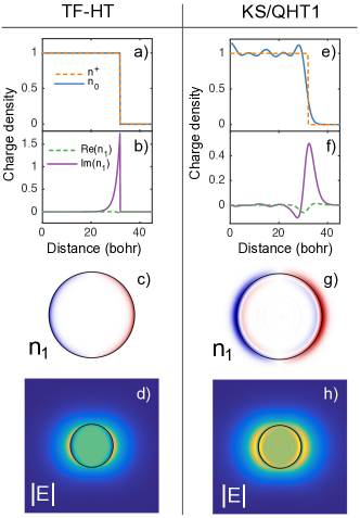
Figure 1: Jellium nanosphere ($r_{s}=4$) with $N_{e}=508$ electrons (R= 31.9 a.u.) as obtained from the TF-HT (panel a,b,c,d) and the KS/QHT1 (panels e,f,g,h) approaches. Ground-state density $n_{0}(r)$, panel a) and e); Real and imaginary part of the induced charge density $n_{1}({\bf r})$ at the plasmon resonance, panel b) and f); Imaginary part of $n_{1}({\bf r})$ at the cross-section plane, panel c) and g); Norm of the induced electric field at the cross-section plane, panel d) and h).

In Fig. 1 we compare the results of the TF-HT approach for a jellium nanosphere with $N_{e}=508$ electrons with the solution of the QHT equations with $\eta=1$ (QHT1) using the exact KS ground-state electronic density; this approach will be referred to as KS/QHT1. While the TF-HT approach assumes that $n_{0}({\bf r})=n^{+}$, see Fig. 1a, the KS ground-state density spreads out from the jellium boundary, see Fig. 1e). The resulting induced density $n_{1}({\bf r})$ from the TF-HT model is confined inside the jellium boundary, see Fig. 1b) and c), whereas there is a significant spill-out in the KS/QHT1 method, see Fig. 1 g) and h), as recently discussed in Ref. Toscano et al., 2015. This difference will lead to a different description of the electric field at the surface, which is the key quantity for plasmonic applications, such as enhancement of the spontaneous emission ratesAkselrod et al. (2014), sensingChen et al. (2015); King et al. (2015), and nonlinear optical effectsCiracì et al. (2015); Argyropoulos et al. (2014).

In the following of the paper, we aim to verify if KS/QHT1 yields correct $n_{1}({\bf r})$ and plasmon energies, and to investigate alternative paths to compute the ground-state density.

IV Input Ground-state Densities

The computation of the KS ground-state density is out-of-reach for all but the smallest systems (computational cost scales as $O(N_{e}^{3})$). An alternative, computationally cheaper but less accurate, is to use OF-DFT to compute the ground-state density ($n_{0}^{\text{OF}}({\bf r})$). In this case we have to solve the Euler equation Parr and Yang (1989):

$$\frac{\delta T_{s}}{\delta n_{0}({\bf r})}+v_{xc}({\bf r})-e\phi({\bf r})=\mu^{\text{OF}}$$ (8)

where $\mu^{\text{OF}}$ is a constant representing the chemical potential and $\phi({\bf r})$ is the total (i.e. from both electrons and the bare positive background) electrostatic potential. The Euler equation (8) can be recast into an eigenvalue equation for the square root of the electron density Levy et al. (1984); if the kinetic energy (KE) is approximated as $T_{s}^{\text{TF}}+(1/\eta_{g})T_{s}^{W}$ it takes the form:

$$\left(\frac{1}{\eta_{g}}\ \frac{\hbar^{2}\nabla^{2}}{2m_{e}}+\frac{\delta T_{s}^{\text{TF}}}{\delta n_{0}({\bf r})}+v_{xc}({\bf r})-e\phi({\bf r})\right)\sqrt{n_{0}({\bf r})}$$

$$\;\;\;\;\;\;\;\;=\mu^{\text{OF}}\sqrt{n_{0}({\bf r})}$$ (9)

which we solved as a self-consistent KS equation (see above), considering only the lowest eigenvalue (with angular momentum $l=0$). The self-consistent calculation of $n_{0}^{\text{OF}}({\bf r})$ can be, in principle, obtained for spherical nanoparticles of any size (computational cost is $O(N_{e})$), even if we experienced very slow convergence, especially for $\eta=9$.

A third approach is to use a model expression that approximates the exact density. For a sphere, the approximated unperturbed electron density can be described by using the modelSnider and Sorbello (1983); Brack (1989); Banerjee and Harbola (2000, 2008):

$$n_{0}^{Mod}({\bf r})=\frac{f_{0}}{1+\exp{\left(\kappa^{\text{Mod}}(r-R)\right)}}$$ (10)

where $r$ is the distance from the center of the sphere and $R$ is the radius of the nanosphere. The expression (10) has to be normalized such that the total charge equals the total number of electron:

$$4\pi\int_{0}^{+\infty}{n_{0}^{\text{Mod}}(r){r^{2}}dr}=\frac{4}{3}\pi{R^{3}}{n^{+}}=N_{e}.$$ (11)

This approach, if successful, is particularly useful to compute the spectral response of arbitrary big systems, since it provides the ground-state density without any computational cost. We underline that Eq. (10) is not employed for a variational calculation of the ground-state densitySnider and Sorbello (1983); Brack (1989); Banerjee and Harbola (2000, 2008). Instead we will fix $\kappa_{\text{Mod}}$, which describes the asymptotic decay of the electronic density and is the only parameter in Eq. (10), as described in the next section.

V Asymptotic Analysis

In the KS or OF approach, if we assume that $v_{s}({\bf r})=v_{xc}({\bf r})-e\phi({\bf r})$ goes exponentially to zero (this is the case for a neutral system and using LDA for the XC functional), then the density asymptotically decays asParr and Yang (1989)

$$n_{0}({\bf r})\rightarrow\frac{A}{r^{2}}\exp(-\kappa r)\;.$$ (12)

In the OF approach, if the KE is approximated as $T_{s}^{\text{TF}}+(1/\eta_{g})T_{s}^{W}$ we have:

$$\kappa^{\text{OF}}=\left(\frac{1}{a_{0}\sqrt{E_{h}}}\right)2\sqrt{-2\mu^{\text{OF}}}\sqrt{\eta_{g}}.$$ (13)

In the KS approach we have Parr and Yang (1989)

$$\kappa^{\text{KS}}=\left(\frac{1}{a_{0}\sqrt{E_{h}}}\right)2\sqrt{-2\epsilon^{{\rm HOMO}}}$$ (14)

and $\epsilon^{{\rm HOMO}}$ is the eigenvalue of the highest occupied molecular orbital (HOMO). Note that $\epsilon^{{\rm HOMO}}<0$ for stable electronic systems and it coincides with the negative of the ionization potential only for the exact XC-functionalPerdew et al. (1982).

The values of $\mu^{\text{OF}1}$ (i.e., OF-DFT with $\eta=1$), $\mu^{\text{OF}9}$ (i.e., OF-DFT with $\eta=9$) and $\epsilon^{{\rm HOMO}}$ for all the jellium nanospheres considered are reported in Fig. 2. It is found that $|\mu^{\text{OF}9}|$ is only a factor 1.1-1.4 smaller than $\mu^{\text{OF}1}$. Thus, unless $\eta_{g}=1$, we have that the density computed in OF-DFT is decaying faster than the exact one, as numerically shown in Fig. 3 for a jellium nanosphere with $N_{e}=338$ electrons. This is consistent with the fact that the von Weizsäcker KE approximation is exact in the asymptotic region Parr and Yang (1989); Della Sala et al. (2015).

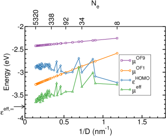
Figure 2: Eigenvalues versus the inverse of the jellium nanosphere ($r_{s}=4$ a.u.) diameter; chemical potential ($\mu^{\rm OF9}$) of orbital-free DFT calculations with $\eta=9$ (purple squares); chemical potential ($\mu^{\rm OF1}$) of orbital-free DFT calculations with $\eta=1$ (orange circles); HOMO eigenvalues ($\epsilon^{{\rm HOMO}}$) of KS-DFT calculations (blue diamonds); effective eigenvalue ($\mu^{\rm eff}$) from the KS-DFT electronic density decay (green triangles), see text for details.

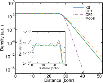
Figure 3: Ground-state electronic density (in a log-scale) for a jellium nanosphere ($r_{s}=4$) with 338 electrons (R=27.8 bohr) computed by KS-DFT, OF-DFT with $\eta_{g}=1$ (OF1) and with $\eta_{g}=9$ (OF9), and the model density. The inset shows the ground-state electronic density in a linear scale inside the nanosphere.

We remark that Eq. (14) is valid only in the asymptotic region, i.e. where the density is dominated only by the HOMO. However, in the case of jellium nanospheres, there are several KS orbitals with energies very close to the HOMO, so that the asymptotic limit will be reached only very far from the jellium boundary, in a region that is not relevant for total energies, nor for the optical properties (see Fig. 4). If in the “near” asymptotic region (i.e. within the simulation domain) we assume that the density decays as in Eq. (12), with $\kappa=\kappa^{\text{eff}}$ then we can define an effective energy:

$$\mu^{\text{eff}}=-(E_{h}a_{0}^{2})\frac{(\kappa^{\text{eff}})^{2}}{8}.$$ (15)

The values of $\mu^{\text{eff}}$ are also reported in Fig. 2, and they are clearly larger (in absolute value) than the $\epsilon^{{\rm HOMO}}$; the difference increases with the number of electrons, due to the increasing contribution of other (low-lying) orbitals. For an infinite number of electrons, a linear extrapolation gives $\mu^{\text{eff},\infty}\approx-3.75$ eV. We then use this value to define

$$\kappa^{\text{Mod}}=\left(\frac{1}{a_{0}\sqrt{E_{h}}}\right)\sqrt{-8\mu^{\text{eff},\infty}}\approx 1.05.$$ (16)

Figure 3 shows that very good agreement is obtained in the asymptotic region, between the model and the KS density.

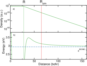
Figure 4: (a) KS Ground-state electronic density $n_{0}({\bf r})$ for a jellium sphere with $N_{e}=338$ electrons ($R=27.86$ bohr, indicated by the solid-blue vertical line) ; (b) Plot of $-(E_{h}a_{0}^{2})\frac{1}{8}\left(\frac{d\ln(r^{2}n_{0}(r))}{dr}\right)^{2}$, which represents the ’local’ $\mu^{\text{eff}}$ in the case of real density. Only in the far asymptotic region (e.g. for $r>150$ bohr) $\mu^{\text{eff}}$ approaches $\epsilon^{{\rm HOMO}}$ indicated by a horizontal green dashed line. In the simulation domain, indicated by the vertical red-line, $\epsilon^{\text{eff}}$ is significantly larger than $\epsilon^{{\rm HOMO}}$.

We now move to consider the asymptotic solution of the QHT$\eta$ equations for spherical systems, extending the work in Ref. Yan, 2015, where only slabs have been considered, and the early one in Ref. Malzacher and Dreizler, 1982. If we assume the ground-state density decay in Eq. (12) then we want to verify if Eq. (4) has solutions of the type

$$n_{1}({\bf r})\rightarrow B\exp(-\beta r)\cos(\theta)$$ (17)

hereby limiting our investigation to dipolar excitations. To proceed, we take the divergence of Eq. (4b), and we use the quasistatic approximation (so that $\varepsilon_{0}\nabla\cdot{\bf E}=\nabla\cdot{\bf P}=en_{1}$), obtaining:

$$\nabla\cdot\frac{{e{n_{0}}}}{{{m_{e}}}}\nabla{\left({\frac{{\delta G}}{{\delta n}}}\right)_{1}}+\left({{\omega^{2}}}\right)en_{1}=-\frac{e^{2}}{m_{e}}\left(\frac{e}{\varepsilon_{0}}n_{0}n_{1}+\nabla n_{0}\cdot{\bf E}\right).$$ (18)

In Eq. (18) we also assume no damping (i.e. $\gamma=0$) and no external field (i.e. we are considering only free oscillations). The asymptotic solution of Eq. (18) can be easily found considering that the second term on the left-hand side is proportional to $n_{1}$: thus all terms which decay exponentially faster than $n_{1}$ can be neglected. These are: the TF and XC contributions in the first term on the left-hand side, which are proportional to $n_{0}^{2/3}n_{1}$ and $n_{0}^{1/3}n_{1}$, respectively (see Eq. (3a) and (3c)), and the first term to the right-hand side (proportional to $n_{0}n_{1}$). The second term on the right-hand side requires special attention. Asymptotically it decays proportionally to $(n_{0}d)/r^{3}$, where $d$ is the dipole moment of $n_{1}$. Thus Eq. (18) has an asymptotic solution only and only if $n_{0}$ decays faster than $n_{1}$, i.e. if

$$\beta<\kappa.$$ (19)

Using Eqs. (12) and (17) in Eq. (18), we obtain (after some algebra) that Eq. (18) is asymptotically satisfied if

$$\left(\frac{E_{h}a_{0}^{2}}{m_{e}}\right)\frac{1}{\eta}\left(\frac{\kappa^{2}\beta^{2}}{4}+\frac{\beta^{4}}{4}-\frac{\kappa\beta^{3}}{2}\right)=\omega^{2}\;\;.$$ (20)

This equation has four solutions of the type:

$$\beta=\frac{\kappa}{2}\pm\frac{\kappa}{2}\sqrt{1\pm\frac{\omega}{\omega_{c}}}$$ (21)

where the critical energy is:

$$\hbar\omega_{c}=\hbar\frac{\kappa^{2}}{8}\sqrt{\left(\frac{E_{h}a_{0}^{2}}{m_{e}}\right)\frac{1}{\eta}}=|\mu|\frac{\eta_{g}}{\sqrt{\eta}}$$ (22)

where we used Eq. (13). Note that it turned out that these solutions are identical to the slab case Yan (2015).

The four solutions are shown in Fig. 5.

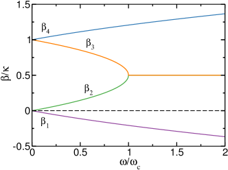
Figure 5: Graphical representation of the solutions in Eq. (21), see text for details.

Solution $\beta_{1}$ is negative, i.e. it is asymptotically increasing, thus it is excluded by the boundary conditions. Solution $\beta_{4}$ is excluded by the condition in Eq. (19). Solution $\beta_{2}$ and $\beta_{3}$ are real only for $\omega<\omega_{c}$. For $\omega>\omega_{c}$, $\beta_{2,3}$ are complex with the real part fixed to $\kappa/2$. The above results are consistent with the TD-DFT calculations of finite systems ($\eta=\eta_{g}=1$), where $\hbar\omega_{c}=\epsilon^{{\rm HOMO}}$ can be interpreted as the ionization threshold Casida et al. (1998). In fact, in TD-DFT the computation of excitation energies higher than $\epsilon^{{\rm HOMO}}$ (i.e. the plasmon peak, too) can be challenging because all the continuum of virtual orbitals must be accurately described. In the same way the spectra calculated within QHT are well convergent up to energy $\hbar\omega_{c}$.

When the sphere is excited by photons with an energy larger than $\hbar\omega_{c}$, we experienced a large dependence on the domain size. This is due to the fact that the induced charge density acquires a propagating characteristic typical of electrons in vacuum. The boundary condition we used (${\bf P}={\bf 0}$) is no longer valid since it produces an artificial scattering of the electrons at the simulation boundary and appropriate boundary conditions should be developedMalzacher and Dreizler (1982); Engquist and Majda (1977). For the jellium nanospheres considered in this work we have that $\mu^{\text{eff}}\approx$ 3.5 eV (see Fig. 2) which is a bit above the Mie energy $\hbar\omega_{Mie}=(E_{h})\sqrt{1/r_{s}^{3}}=$3.4 eV. Numerically we found that only the calculation of the main (first) plasmon peak is stable.

VI Plasmon Resonance and Spill-out Effects.

In Fig. 6 we plot the absorption cross-section, $\sigma$, normalized to the geometrical area $\sigma_{0}=\pi R^{2}$, for a Na jellium sphere ($r_{s}=4$ a.u.) with $N_{e}=338$ and thus $R=27.86$ a.u. ($D=2.94$ nm), using different approaches.

Figure 6a) reports the reference TD-DFT results. TD-DFT calculations (in the adiabatic LDA) have been performed using an in-house developed code, following the literature Zangwill and Soven (1980); Ekardt (1985); Bertsch (1990); Prodan and Nordlander (2002). Details of our TD-DFT numerical implementation, which allows calculations for large nanospheres will be discussed elsewhere. In TD-DFT (where no retardation is included) the absorption cross-section can be computed as:

$$\sigma(\omega)=\frac{\omega}{c\varepsilon_{0}}{\rm Im}\left[\alpha_{zz}(\omega)\right]\;\;,$$ (23)

where the frequency dependent polarizability is:

$$\alpha_{zz}(\omega)=-e^{2}\int{\rm d}{\bf r}{\rm d}{\bf r}^{\prime}z\chi({\bf r},{\bf r}^{\prime},\omega)z^{\prime}\;\;,$$ (24)

and $\chi({\bf r},{\bf r}^{\prime},\omega)={\delta n({\bf r})}/{\delta(eV_{ext}({\bf r}^{\prime}))}$ is the interacting density response function Ullrich (2011).

Panels b), c) and d) of Fig. 6 report the QHT absorption cross section computed as:

$$\sigma(\omega)=\frac{1}{I_{0}}\frac{\omega}{2}\int{{\mathop{\rm Im}\nolimits}\left\{{{\bf{E}}\cdot{{\bf{P}}^{*}}}\right\}dV}$$ (25)

where $I_{o}$ is the energy flux of the incident plane-wave.

Panel 6b) shows the spectrum obtained by applying the QHT method with $\eta=9$ (QHT9) to the OF9 density; this approach will be called self-consistent OF9/QHT9 and coincides with the approach of Toscano et al.Toscano et al. (2015), with the only difference being the choice of the XC functional. The energy position of the first peak ($\approx$ 3.2eV) is in very good agreement with the TD-DFT result ($\approx$ 3.15eV). Obviously TD-DFT results are much broadened due to quantum size effects as $N_{e}$ is quite small. However, the decay of $n_{1}$ is very different from the reference TD-DFT results. In fact from Eq. (22) we obtain that $\hbar\omega_{c}=3|\mu^{{\text{OF}}9}|$. From Fig. 2 we see that $\mu^{{\text{OF}}9}\approx-2.4$ eV and thus the critial frequency is artificially moved to very high energy ($\hbar\omega_{c}\approx 7.2$ eV). A good point of the OF9/QHT9 approach is that the computation of all the spectrum (i.e. up to 7.2 eV) will be numerically stable. On the other hand, from Eqs. (21) and (13) we see that the first solution will have a decay $\beta^{{\text{OF}}9/{\rm QHT}9}\approx 0.87\kappa^{{\text{OF}}9}\approx 2.61\kappa^{\text{KS}}$, i.e. much more confined than the reference TD-DFT results, as numerically shown in Fig. 7. Recall that in TD-DFT the induced density will also decay as in Eq. (17) with $\kappa^{\text{KS}}/2\leq\beta\leq\kappa^{\text{KS}}$ as discussed in Ref. Yan et al., 2015. The so-called spill-out effects in computational plasmonics, which indeed refer to the profile of induced density, are thus largely underestimated in the OF9/QHT9 approach. Thus the good accuracy of the OF9/QHT9 resonance energy seems originating from error cancellation between between the too confined ground-state electron density (from OF9) and the approximated kinetic energy-kernel (QHT9, which is valid only for slowly varying density).

In Fig. 6c) we report the results from the KS/QHT1 approach, already introduced in Fig. 1. In this case the resonance peak ($\approx$ 3.13 eV) is in even better agreement with the TD-DFT results. Almost the same results are obtained by applying the QHT1 method to the model ground-state density (Mod/QHT1), as shown in Fig. 6d). More importantly Fig. 7 shows that the induced density $n_{1}$ from KS/QHT1 has almost the same decay of the TD-DFT result, i.e. the KS/QHT1 approach correctly describes the spill-out effects of the induced charge density.

It is useful to remark that, despite the fact the all the spectra presented in Fig. 6b-d) result quite similar, QHT is very sensible to the density tail. Using a model density with a larger (smaller) $\kappa^{\text{Mod}}$ yields a red-shifted (blue-shifted) plasmon peak. In a similar way, using the QHT1 method with the OF1 ground-state density yields a plasmon peak red-shifted by about 0.3 eV (data not reported). This is not surprising considering that the OF1 density is decaying much more slowly than the effective one, see Fig. 2. As mentioned at the end of Section V, spectral features appearing at energies higher than the ionization energy ($\hbar\omega_{c}$) are not stable and will be investigated elsewhere. We also point out that QHT with $\eta=9$ (which yields the exact dielectric response for small wavevectorsAkbari-Moghanjoughi (2015)) cannot be used in combination with a ground-state density with the exact asymptotic decay. This seems surprising, but it can be easily justified by looking at Eq. (22). If $\eta_{g}=1$ and $\eta=9$ we obtain $\hbar\omega_{c}=|\mu^{\text{eff}}|/3\approx 1.16eV$, i.e. the critical frequency is three times smaller than the Mie frequency, so that the whole absorption spectrum can be hardly computed.

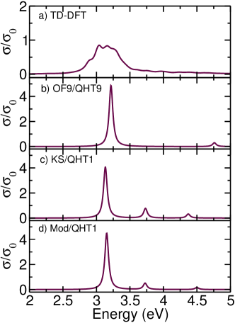
Figure 6: Absorption cross section ($\sigma$) normalized to the geometrical area ($\sigma_{0}$) for a jellium nanosphere ($r_{s}=$ 4 a.u.) with $N_{e}=338$ electrons as obtained form TD-DFT, OF9/QHT9, KS/QHT1 and Mod/QHT1. All the spectra have been obtained using an empirical broadening of 0.066 eV.

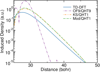
Figure 7: Induced density (complex modulus of $n_{1}$) at the plasmon energy for a jellium nanosphere ($r_{s}$=4 a.u.) with $N_{e}=338$ electrons ($R=27.86$ bohr), as computed from TD-DFT, OF9/QHT9, KS/QHT1 and Mod/QHT1.

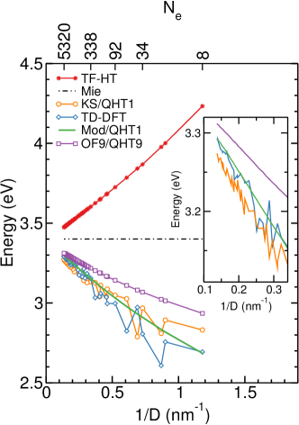
Figure 8: Plasmon resonance for jellium nanospheres ($r_{s}$=4 a.u.) as a function of the inverse of the sphere diameter, as computed by different approaches. The behavior for large particles is shown in the inset.

We now move on to describe the shift of the plasmon resonance as a function of the particle size. This problem has been extensively studied in the literature, both theoreticallyRuppin (1978); Yannouleas et al. (1993) and experimentallyReiners et al. (1995); Parks and Mcdonald (1989); Scholl et al. (2012), and it represents a relevant benchmark for estimating the accuracy of QHT. In Fig. 8 we report the energy position of the main resonance peak as a function of the inverse of the jellium nanosphere diameter, $D$. The exact energy position of the main peak has been extracted from the computed spectra (with an empirical broadening of $\hbar\gamma=0.1$ eV and using a spline interpolation). These procedure is not unique for some of the smallest clusters, where there are many peaks with similar intensity (for large cluster there is always an unique main peak).

The dot-dashed horizontal line represents the Mie plasmon energy ($\hbar\omega_{Mie}=3.4$ eV). Note that for the diameters considered in Fig. 8, retardation effects can be neglected.

The first thing to notice is the striking difference obtained using TF-HT. It predicts in fact a resonance shift toward higher energies (shorter wavelengths) as the particle radius gets smaller, as previously observed in other systemsRaza et al. (2011); Toscano et al. (2012); Raza et al. (2013). For all the other cases the peak resonances slide to lower energies (longer wavelengths) as the particle radius shrinks. While for noble metals like Au or Ag the plasmon resonance undergoes a blue shift as the radius $R$ decreasesBorensztein et al. (1986); Lermé et al. (1998), this is not the case for Na. The origin of the blue shift for noble metal nanoparticles is due to size dependent changes of the optical interband transitions Liebsch (1993); Monreal et al. (2013).

We now compare the QHT models investigated in this work, with respect to the TD-DFT results, which can be considered as a reference. As widely investigated in the literature for jellium nanospheresYannouleas et al. (1993), the TD-DFT main peak oscillates for small $N_{e}$, but it converges to $\hbar\omega_{Mie}$ for large $N_{e}$.

Results for the OF9/QHT9 approach are significantly blue-shifted with respect to TD-DFT (note that OF9/QHT9 predicts a red-shift with respect to TF-HT, as also found in Ref. 75), and do not present quantum oscillations. In fact, it is well knownHohenberg and Kohn (1964) that orbital-free (OF1 or OF9) electronic density does not show quantum (i.e. Friedel) oscillations inside the nanosphere (see inset of Fig. 3). On the other hand when QHT1 is applied to the KS density, quantum-oscillations are clearly visible for small nanospheres, even if TD-DFT features are not fully reproduced. For $N_{e}\geq 338$, KS/QHT1 reproduces TD-DFT plasmon energies with great accuracy (with a maximum error of 20 meV, about a half of the error obtained with the OF9/QHT9 approach, see Table S1 in the Supplemental Material).

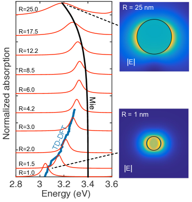
Figure 9: Mod/QHT1 spectra for jellium nanospheres ranging from $R=2$ to 25 nm (red curves). The black (blue) curve shows the Mie (TD-DFT) resonance trajectory.

Finally, we analyze results for Mod/QHT1. Also in this case no quantum-oscillations are present, and for $N_{e}\geq 338$ TD-DFT results are reproduced almost exactly, with a maximum error of only 10 meV. Thus using a simple model density it is possible to match the whole range of nanoparticle sizes. The comparison between TD-DFT and KS/QHT1 is important because both approaches use the same KS density (in the former additional information is used from the KS orbital and eigenvalues). The good accuracy in Fig. 8 means that for large nanospheres the full TD-DFT linear response can be well approximated by the simpler QHT1 method. The very good results obtained for Mod/QHT1 are even more important. In fact it means that QHT can be use without the need of calculating the KS ground-state density, which is a bottleneck for large system (scales as $O(N_{e}^{3})$). Moreover, the simple model density employed here can be constructed at no cost for systems of any size, and can also be generalized to the non-spherical case. The parameter $\kappa^{\text{Mod}}$, is clearly material-dependent (e.g. will depend on $r_{s}$) but can be parameterized once and for all.

In Fig. 9 we show the absorption spectrum for particles with a diameter going from 2 up to 50 nm. The solid black line shows the trajectory of the Mie resonance as the particle size increases: for particles with $R>10$ nm the Mie resonance peak undergoes a red-shift due to retardation effects. The red curves represent the spectrum calculated within the Mod/QHT1 method. For small nanoparticles the peaks follow the TD-DFT trajectory, moving toward higher energies. As the particle size grows the plasmon energy tends toward the Mie trajectory, up to the big particle regime, where retardation effects become predominant (see Fig. 8). It is striking how Mod/QHT1 can describe the full range of effects going from the nonlocal/spill-out effects up to retardation effects. That is, the resonance shift due to microscopic and macroscopic effects are incorporated in a single model, which makes the potential of QHT with respect to DFT approach very clear. Although this advantage was already outlined by the authors of Ref. 75, we remark that their method was only qualitatively verified for nanowires.

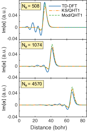
Figure 10: Induced polarization charge density (normalized by $R^{3}$) at the plasmonic resonance $\omega_{0}$ for different jellium nanospheres.

VII The induced charge density

So far we have seen that KS/QHT1 or Mod/QHT1 reproduce with very good accuracy the reference TD-DFT results, both the energy position and the asymptotic decay of the induced density. In this section we closely analyze the near-field properties. Accurate induced density translates into a good description of the local fields at the surface of the plasmonic system. Such knowledge is crucial for estimating the maximum field enhancements, and hence nonlinear optical efficiencies, and more in general light-matter interactions.

In particular we compare the QHT1 induced polarization charge density to the full TD-DFT calculations. The polarization charge density $\alpha_{zz}(r)$ of a sphere excited by the incident field ${\bf E}_{0}={\bf\hat{z}}E_{0}$ can be defined from:

$$n_{1}(r,\theta,\phi)=-eE_{0}\frac{1}{r^{2}}\cos(\theta)\alpha_{zz}(r,\omega)$$ (26)

so that

$$\alpha_{zz}(\omega)=\frac{4\pi}{3}\int_{0}^{+\infty}{\alpha_{zz}(r,\omega)}rdr.$$ (27)

In Fig. 10 we plot the imaginary part of the induced polarization charge density for different particles sizes in correspondence with the plasmon resonance $\omega_{0}$. For the smaller particles big oscillations of the density can be seen in the case of the TD-DFT calculations that are not present if not in a very modest from in the case of QHT1. These oscillations are in fact due to a purely quantum size effect (Friedel oscillations). As the particle size increases however, these oscillations diminish. The main induced peak, however, is very well reproduced by the QHT1 approach, both with the KS or the model ground-state density.

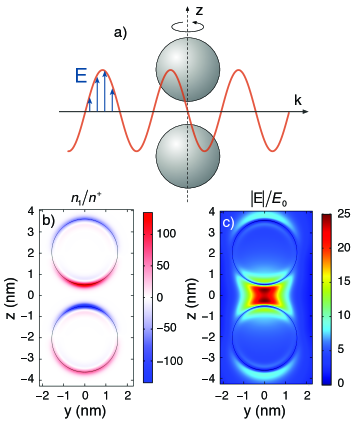
Figure 11: Dimer of Na spheres constituted by $N_{e}=398$ electrons each, and separated by a distance $g=1$ nm. The dimer is excited by a plane wave oscillating with energy $\hbar\omega=-2.8$ eV, $\gamma=\gamma_{0}+v_{F}/R$ has been used with $\hbar\gamma_{0}=0.066$ eV. (a) Geometry and incident field. (b) Real part of the induced charge density normalized with respect to the bulk positive charge density. (c) Electric field norm distribution.

VIII Application to the sphere dimer

Up to this point we have considered spheres. In this section we are going to extend the applicability of QHT to axially symmetric structures. Our 2.5D implementation (see Appendix A) makes this task really easy and the only difference is in the excitation field. Because the response of a spherical system is independent from the direction and polarization of the incident wave, in the previous calculations we have assumed for convenience a plane wave propagating along the $z$ axis so that we would need to solve our equations just for the cylindrical harmonic with azimuthal number $m=1$ (the case for $m=-1$ can be obtained by taking into account field parities). For axis-symmetric structures, in general, it is not possible to arbitrarily choose the incident wave and it becomes necessary to solve the problem for several azimuthal numbers. For sub-wavelength structures, however, the number of cylindrical harmonics $m_{max}$ needed to accurately describe the problem remains very small ($m_{max}<3$).

A relevant example of axially symmetric structure is the sphere dimer. This structure has been extensively studied in the literature for its ability to strongly enhance local electric fields with respect to the incident radiationRomero et al. (2006); Fernández-Domínguez et al. (2012b, 2010) and its potential to exhibit quantum effectsZuloaga et al. (2009); Marinica et al. (2012a); Barbry et al. (2015a). Here, we consider a dimer of Na spheres constituted by $N_{e}=398$ electrons each, and separated by a distance $g=1$ nm. The dimer is excited by a plane wave propagating orthogonally to the dimer axis whose electric field is polarized along $z$ (as depicted in Fig. 11a) and is oscillating with energy $\hbar\omega=-2.8$ eV. In Fig. 11b-c we plot the induced charge density and the electric field norm respectively for the case of Mod/QHT1 where the same equilibrium charge density as the single particle case has been used. Although, our TD-DFT implementation can only be applied to spheres, Fig. 11 and in particular Fig. 11c can be directly compared to results of Ref.28 in which TD-DFT calculations for the same jellium Na dimer are reported. It can be seen that the electric field distribution in the gap and in the vicinity of the jellium edge is accurately reproduced both qualitatively and quantitatively.

It is worth noting that results obtained with Mod/QHT1 are valid as long as the equilibrium electron density of a dimer can be approximated to that obtained by summing the densities of two single spheres. For very small gaps ($g<0.4$ nm) this is not necessarily true and particular attention needs to be paid to the choice of the equilibrium density in the overlapping region.

IX Conclusion

In this work, we have investigated how different models based on QHT can describe the plasmonic properties of spherical nanoparticles in comparison with reference TD-DFT results.

The main finding is twofold:

• The accuracy of QHT strongly depends on the choice of the ground state density. In particular the self-consistent approach with $\eta=9$ produces correct results only for the plasmon resonance energy, whereas the induced density spill-out is largely underestimated. Using the exact KS electron equilibrium density within the QHT method with the full von Weizsäcker kinetic energy, allows to predict the plasmon energy for Na jellium nanospheres within an error of about 20 meV in comparison with TD-DFT predictions.

• QHT yields similar high accuracy (with a maximum error of only 10 meV) if an analytical model density with the correct asymptotic behavior is used (the Mod/QHT1 approach). This finding is of utmost importance because it allows to circumvent the bottleneck given by the necessity of computing the exact KS ground state density, allowing the QHT method to be directly applied to macroscopic systems that still require a precise microscopic description, such as gap-plasmon structuresSavage et al. (2012); Hajisalem et al. (2014); Ciracì et al. (2012).

By using a finite-element implementation based on the 2.5D technique we were able to investigate spherical nanoparticles under a plane-wave excitation and extend our calculations to big particles maintaining retardation effects. We showed that our implementation can be used to study nanoparticle dimers and in general can be applied to arbitrary geometries that possess axial symmetry, such as cones, nanoparticle dimers, disks, or film-coupled nanoparticles. These systems are in fact quite frequent in experimental setups.

We believe that Mod/QHT1 is quite promising and can be further improved by adding extra termsYan (2015) and more accurate kinetic energy functionalsLaricchia et al. (2014) in order to be more reliable toward UV frequencies and for describing valence electrons in noble metals, for which a dynamical kinetic energy functional might be necessary. Although the QHT approach is not suitable to directly describe interband processes, these can be approximately taken into account by considering a local polarizability contribution Liebsch (1993); Toscano et al. (2015). Moreover, QHT can be straightforwardly generalized to higher order terms so that nonlinear optical effects that are generated at the surface of a plasmonic system can be included in the calculations.

Appendix A Numerical implementation of the QHT

We solved the system of Eqs. (4) using a commercially available software based on Finite-element method (FEM): Comsol MultiphysicsComsol Multiphysics . The problem $L{\bf u}={\bf 0}$, where $L$ is a linear differential operator and ${\bf u}$ the independent variable vector can be described by means of the weak formulation:

$$\int{{L_{1}}{\bf{u}}\cdot{L_{2}}{\bf{v}}}dV=0,$$ (28)

where ${\bf v}$ is a test function and the operators $L_{1}$ and $L_{2}$ are linear operators containing derivatives of order smaller than $L$. In general, it is possible to go from $L$ to $L_{1}$ and $L_{2}$ simply by integrating by parts. In FEM this step is necessary since one wants to keep the functions ${\bf u}_{i}$ approximating the solution ${\bf u}\simeq\sum_{i}\alpha_{i}{\bf u}_{i}$ as simple as possible.

In the case of the Eq. (4b) we obtain integrating by parts and assuming the integral on the boundary to be equal zero the following weak expression:

$$\int{-{\frac{e}{{{m_{e}}}}{{\left({\frac{{\delta G}}{{\delta n}}}\right)}_{1}}\left({\nabla\cdot{\bf{\tilde{P}}}}\right)+\frac{1}{{{n_{0}}}}\left[{\left({{\omega^{2}}+i\gamma\omega}\right){\bf{P}}+{\varepsilon_{0}}\omega_{p}^{2}{\bf{E}}}\right]\cdot{\bf{\tilde{P}}}}}dV=0,$$ (29)

where we distributed the derivatives to the test functions ${\bf{\tilde{P}}}$. This allows us to avoid calculating the gradient of the energy functional of Eq. (6). However, since the expression of the energy functional contains second order derivatives, we introduce the working variable ${\bf F}=\nabla n_{1}$ with $n_{1}=\frac{1}{e}\nabla\cdot{\bf P}$, so that $\nabla^{2}n_{1}=\nabla\cdot{\bf F}$, and our system of equations contains only first order derivatives.

In order to take advantage from the symmetry of the geometry, we implemented our equations assuming an azimuthal dependence of the form $e^{-im\phi}$ with $m\in\mathbb{Z}$. That is, for a vector field ${\bf v}$, we have ${\bf v}(\rho,\phi,z)=\sum_{m\in\mathbb{Z}}{\bf v}^{(m)}(\rho,z)e^{-im\phi}$. Maxwell’s equation and the polarization equation are written assuming the following definitions:

$$\nabla\cdot{{\bf{v}}^{(m)}}\equiv\left({\frac{1}{\rho}+\frac{\partial}{{\partial\rho}}}\right)v_{\rho}^{(m)}-\frac{{im}}{\rho}v_{\phi}^{(m)}+\frac{{\partial v_{z}^{(m)}}}{{\partial z}},$$

$$\begin{array}[]{l}\nabla\times{{\bf{v}}^{(m)}}\equiv\hat{\rho}\left({-\frac{{\partial v_{\phi}^{(m)}}}{{\partial z}}-i\frac{m}{\rho}v_{z}^{(m)}}\right)+\\ \quad+\hat{\phi}\left({\frac{{\partial v_{\rho}^{(m)}}}{{\partial z}}-\frac{{\partial v_{z}^{(m)}}}{{\partial\rho}}}\right)+\hat{z}\left({\frac{{v_{\phi}^{(m)}}}{\rho}+\frac{{\partial v_{\phi}^{(m)}}}{{\partial\rho}}+i\frac{m}{\rho}v_{\rho}^{(m)}}\right)\end{array}$$

Analogously, the test functions are assumed to have a dependence of the form $e^{im\phi}$. It is possible then to reduce the initially three-dimensional problem into $(2m_{max}+1)$ two-dimensional problems. The system to solve in the unknown variables ${\bf E}$ (electric field), ${\bf P}$ (polarization field) and ${\bf F}$ (working variable), reads:

$$\begin{array}[]{l}2\pi\int{\left({\nabla\times{{\bf{E}}^{(m)}}}\right)\cdot\left({\nabla\times{{{\bf{\tilde{E}}}}^{(m)}}}\right)-\left({k_{0}^{2}{{\bf{E}}^{(m)}}+{\mu_{0}}{\omega^{2}}{{\bf{P}}^{(m)}}}\right)\cdot{{{\bf{\tilde{E}}}}^{(m)}}}\rho d\rho dz=0,\\ 2\pi\int{-\frac{e}{{{m_{e}}}}\left({\frac{{\delta G}}{{\delta n}}}\right)_{1}^{(m)}\left({\nabla\cdot{{{\bf{\tilde{P}}}}^{(m)}}}\right)+\frac{1}{{{n_{0}}}}\left[{\left({{\omega^{2}}+i\gamma\omega}\right){{\bf{P}}^{(m)}}+{\varepsilon_{0}}\omega_{p}^{2}\left({{{\bf{E}}^{(m)}}+{\bf{E}}_{inc}^{(m)}}\right)}\right]\cdot{{{\bf{\tilde{P}}}}^{(m)}}}\rho d\rho dz=0,\\ 2\pi\int{-\left({\nabla\cdot{{\bf{P}}^{(m)}}}\right)\left({\nabla\cdot{{{\bf{\tilde{F}}}}^{(m)}}}\right)-e{{\bf{F}}^{(m)}}\cdot{{{\bf{\tilde{F}}}}^{(m)}}}\rho d\rho dz=0.\end{array}$$

Note that for the case of an incident plane wave propagating along the $z$ axis, one has to solve the problem just for $m=\pm 1$. Moreover by taking into account field parities, the solution for $m=1$ can be related to the solution for $m=-1$, so that a single two-dimensional calculation becomes necessaryCiracì et al. (2013b, c).

Note that for the electromagnetic module Comsol uses by default curl elements for the in-plane components and Lagrange elements for the azimuthal component. We found that using Lagrange elements for each component provides much more stable solutions. Since Comsol does not give the possibility to use different type of elements for the built-in physics (in our case electromagnetism) we had to re-implement the electromagnetic module ourselves by using the general weak form implementation. Perfectly matched layers have been used in order to emulate an infinite domain and avoid unwanted reflections.

References

- Gramotnev and Bozhevolnyi (2010) D. K. Gramotnev and S. I. Bozhevolnyi, “Plasmonics beyond the diffraction limit,” Nat. Photonics 4, 83 (2010).
- Schuller et al. (2010) J. A. Schuller, E. S. Barnard, W. Cai, Y. C. Jun, J. S. White, and M. L. Brongersma, “Plasmonics for extreme light concentration and manipulation,” Nat. Mater. 9, 193 (2010).
- Maier (2007) S. A. Maier, Plasmonics, Fundamentals and Applications (Springer, 2007).
- Aouani et al. (2014) H. Aouani, M. Rahmani, M. Navarro-Cía, and S. A. Maier, “Third-harmonic-upconversion enhancement from a single semiconductor nanoparticle coupled to a plasmonic antenna,” Nat. Nanotechnol. 9, 290 (2014).
- Moreau et al. (2012) A. Moreau, C. Ciracì, J. J. Mock, R. T. Hill, Q. Wang, B. J. Wiley, A. Chilkoti, and D. R. Smith, “Controlled-reflectance surfaces with film-coupled colloidal nanoantennas,” Nature 492, 86 (2012).
- Akselrod et al. (2014) G. M. Akselrod, C. Argyropoulos, T. B. Hoang, C. Ciracì, C. Fang, J. Huang, D. R. Smith, and M. H. Mikkelsen, “Probing the mechanisms of large Purcell enhancement in plasmonic nanoantennas,” Nat. Photonics 8, 835 (2014).
- Akselrod et al. (2015) G. M. Akselrod, T. Ming, C. Argyropoulos, T. B. Hoang, Y. Lin, X. Ling, D. R. Smith, J. Kong, and M. H. Mikkelsen, “Leveraging Nanocavity Harmonics for Control of Optical Processes in 2D Semiconductors,” Nano Lett. 15, 3578 (2015).
- Rose et al. (2014) A. Rose, T. B. Hoang, F. McGuire, J. J. Mock, C. Ciracì, D. R. Smith, and M. H. Mikkelsen, “Control of radiative processes using tunable plasmonic nanopatch antennas,” Nano Lett. 14, 4797 (2014).
- Ciracì et al. (2012) C. Ciracì, R. Hill, J. J. Mock, and Y. A. Urzhumov, “Probing the ultimate limits of plasmonic enhancement,” Science 337, 1072 (2012).
- Savage et al. (2012) K. J. Savage, M. M. Hawkeye, R. Esteban, and A. G. Borisov, “Revealing the quantum regime in tunnelling plasmonics,” Nature 491, 574 (2012).
- Hajisalem et al. (2014) G. Hajisalem, M. S. Nezami, and R. Gordon, “Probing the quantum tunneling limit of plasmonic enhancement by third harmonic generation,” Nano Lett. 14, 6651 (2014).
- Moreau et al. (2013) A. Moreau, C. Ciracì, and D. R. Smith, “Impact of nonlocal response on metallodielectric multilayers and optical patch antennas,” Phys. Rev. B 87, 045401 (2013).
- Chen et al. (2013) X. Chen, H.-R. Park, M. Pelton, X. Piao, N. C. Lindquist, H. Im, Y. J. Kim, J. S. Ahn, K. J. Ahn, N. Park, D.-S. Kim, and S.-H. Oh, “Atomic layer lithography of wafer-scale nanogap arrays for extreme confinement of electromagnetic waves,” Nature Commun. 4, 2361 (2013).
- Chen et al. (2015) X. Chen, C. Ciracì, D. R. Smith, and S.-H. Oh, “Nanogap-enhanced Infrared Spectroscopy with Template-stripped Wafer-scale Arrays of Buried Plasmonic Cavities,” Nano Lett. 15, 107 (2015).
- Ciracì et al. (2014) C. Ciracì, X. Chen, J. J. Mock, F. McGuire, X. Liu, S.-H. Oh, and D. R. Smith, “Film-coupled nanoparticles by atomic layer deposition: Comparison with organic spacing layers,” Appl. Phys. Lett. 104, 023109 (2014).
- Marinica et al. (2012a) D. C. Marinica, A. K. Kazansky, and P. Nordlander, “Quantum plasmonics: nonlinear effects in the field enhancement of a plasmonic nanoparticle dimer,” Nano Lett. 12, 1333 (2012a).
- Zuloaga et al. (2009) J. Zuloaga, E. Prodan, and P. Nordlander, “Quantum Description of the Plasmon Resonances of a Nanoparticle Dimer,” Nano Lett. 9, 887 (2009).
- Ullrich (2011) C. A. Ullrich, ed., Time-Dependent Density-Functional Theory: Concepts and Applications (Oxford University Press, 2011).
- Yabana and Bertsch (1996) K. Yabana and G. F. Bertsch, “Time-dependent local-density approximation in real time,” Phys. Rev. B 54, 4484 (1996).
- Andrade et al. (2012) X. Andrade, J. Alberdi-Rodriguez, D. A. Strubbe, M. J. T. Oliveira, F. Nogueira, A. Castro, J. Muguerza, A. Arruabarrena, S. G. Louie, A. Aspuru-Guzik, A. Rubio, and M. A. L. Marques, “Time-dependent density-functional theory in massively parallel computer architectures: the octopus project,” J. Phys. Condens. Matter 24, 233202 (2012).
- Casida (1996) M. E. Casida, in Recent developments and applications of modern density functional theory, edited by J. M. Seminario (Elsevier, Amsterdam, 1996) pp. 391–434.
- Morton et al. (2011) S. M. Morton, D. W. Silverstein, and L. Jensen, “Theoretical studies of plasmonics using electronic structure methods,” Chem. Rev. 111, 3962 (2011).
- Brack (1993) M. Brack, “The physics of simple metal clusters: self-consistent jellium model and semiclassical approaches,” Rev. Mod. Phys. 65, 677 (1993).
- Ekardt (1985) W. Ekardt, “Size-dependent photoabsorption and photoemission of small metal particles,” Phys. Rev. B 31, 6360 (1985).
- Teperik et al. (2013) T. V. Teperik, P. Nordlander, J. Aizpurua, and A. G. Borisov, “Robust subnanometric plasmon ruler by rescaling of the nonlocal optical response,” Phys. Rev. Lett. 110, 263901 (2013).
- Yan et al. (2015) W. Yan, M. Wubs, and N. Asger Mortensen, “Projected Dipole Model for Quantum Plasmonics,” Phys. Rev. Lett. 115, 137403 (2015).
- Esteban et al. (2012) R. Esteban, A. G. Borisov, and P. Nordlander, “Bridging quantum and classical plasmonics with a quantum-corrected model,” Nature Commun. 3, 825 (2012).
- Barbry et al. (2015a) M. Barbry, P. Koval, F. Marchesin, R. Esteban, A. G. Borisov, J. Aizpurua, and D. Sanchez-Portal, “Atomistic near-field nanoplasmonics: Reaching atomic-scale resolution in nanooptics,” Nano Lett. 15, 3410 (2015a).
- Zhang et al. (2014) P. Zhang, J. Feist, A. Rubio, P. García-González, and F. J. García-Vidal, “Ab initio nanoplasmonics: The impact of atomic structure,” Phys. Rev. B 90, 161407 (2014).
- Li et al. (2013) J.-H. Li, M. Hayashi, and G.-Y. Guo, “Plasmonic excitations in quantum-sized sodium nanoparticles studied by time-dependent density functional calculations,” Phys. Rev. B 88, 155437 (2013).
- Iida et al. (2014) K. Iida, M. Noda, K. Ishimura, and K. Nobusada, “First-principles computational visualization of localized surface plasmon resonance in gold nanoclusters,” J. Phys. Chem. A 118, 11317 (2014).
- Pitarke et al. (2007) J. M. Pitarke, V. M. Silkin, E. V. Chulkov, and P. M. Echenique, “Theory of surface plasmons and surface-plasmon polaritons,” Rep. Prog. Phys. 70, 1 (2007).
- Raza et al. (2011) S. Raza, G. Toscano, A. P. Jauho, M. Wubs, and N. A. Mortensen, “Unusual resonances in nanoplasmonic structures due to nonlocal response,” Phys. Rev. B 84, 121412 (2011).
- Ciracì et al. (2013a) C. Ciracì, J. B. Pendry, and D. R. Smith, “Hydrodynamic Model for Plasmonics: A Macroscopic Approach to a Microscopic Problem,” ChemPhysChem 14, 1109 (2013a).
- Raza et al. (2015) S. Raza, S. I. Bozhevolnyi, M. Wubs, and N. A. Mortensen, “Nonlocal optical response in metallic nanostructures,” J. Phys. Condens. Matter 27, 183204 (2015).
- Parr and Yang (1989) R. G. Parr and W. Yang, eds., Density Functional Theory of Atoms and Molecules (Oxford University Press, 1989).
- Heinrichs (1973) J. Heinrichs, “Hydrodynamic Theory of Surface-Plasmon Dispersion,” Phys. Rev. B 7, 3487 (1973).
- Eguiluz et al. (1975) A. Eguiluz, S. Ying, and J. Quinn, “Influence of the electron density profile on surface plasmons in a hydrodynamic model,” Phys. Rev. B 11, 2118 (1975).
- Eguiluz and Quinn (1976) A. Eguiluz and J. Quinn, “Hydrodynamic model for surface plasmons in metals and degenerate semiconductors,” Phys. Rev. B 14, 1347 (1976).
- Ruppin (1975) R. Ruppin, “Optical properties of small metal spheres,” Phys. Rev. B 11, 2871 (1975).
- Ruppin (1978) R. Ruppin, “Plasmon frequencies of small metal spheres,” J. Phys. Chem. Solids 39, 233 (1978).
- Dasgupta and Fuchs (1981) B. B. Dasgupta and R. Fuchs, “Polarizability of a small sphere including nonlocal effects,” Phys. Rev. B 24, 554 (1981).
- Mock et al. (2008) J. J. Mock, R. Hill, A. Degiron, S. Zauscher, A. Chilkoti, and D. R. Smith, “Distance-dependent plasmon resonant coupling between a gold nanoparticle and gold film,” Nano Lett. 8, 2245 (2008).
- Hill et al. (2010) R. Hill, J. J. Mock, Y. A. Urzhumov, and D. S. Sebba, “Leveraging nanoscale plasmonic modes to achieve reproducible enhancement of light,” Nano Lett. 10, 4150 (2010).
- Mortensen et al. (2014) N. A. Mortensen, S. Raza, M. Wubs, T. Søndergaard, and S. I. Bozhevolnyi, “A generalized non-local optical response theory for plasmonic nanostructures,” Nat. Commun. 5, 3809 (2014).
- Toscano et al. (2013) G. Toscano, S. Raza, W. Yan, C. Jeppesen, and S. Xiao, “Nonlocal response in plasmonic waveguiding with extreme light confinement,” Nanophotonics 2, 161 (2013).
- Filter et al. (2014) R. Filter, C. Bösel, G. Toscano, F. Lederer, and C. Rockstuhl, “Nonlocal effects: relevance for the spontaneous emission rates of quantum emitters coupled to plasmonic structures ,” Opt. Lett. 39, 6118 (2014).
- Ciracì et al. (2013b) C. Ciracì, Y. A. Urzhumov, and D. R. Smith, “Effects of classical nonlocality on the optical response of three-dimensional plasmonic nanodimers,” J. Opt. Soc. Am. B 30, 2731 (2013b).
- Fernández-Domínguez et al. (2012a) A. I. Fernández-Domínguez, P. Zhang, Y. Luo, S. A. Maier, F. J. García-Vidal, and J. B. Pendry, “Transformation-optics insight into nonlocal effects in separated nanowires,” Phys. Rev. B 86, 241110 (2012a).
- Christensen et al. (2014) T. Christensen, W. Yan, S. Raza, A.-P. Jauho, N. A. Mortensen, Morte, and M. Wubs, “Nonlocal Response of Metallic Nanospheres Probed by Light, Electrons, and Atoms,” ACS Nano 8, 1745 (2014).
- Luo et al. (2013) Y. Luo, A. I. Fernandez-Dominguez, A. Wiener, and S. A. Maier, “Surface plasmons and nonlocality: A simple model,” Phys. Rev. Lett. 111, 093901 (2013).
- Wiener et al. (2013) A. Wiener, A. I. Fernández-Domínguez, J. B. Pendry, A. P. Horsfield, and S. A. Maier, “Nonlocal propagation and tunnelling of surface plasmons in metallic hourglass waveguides,” Opt. Express 21, 27509 (2013).
- Wiener et al. (2012) A. Wiener, A. I. Fernandez-Dominguez, and A. P. Horsfield, “Nonlocal effects in the nanofocusing performance of plasmonic tips,” Nano Lett. 12, 3308 (2012).
- Stella et al. (2013) L. Stella, P. Zhang, and F. J. García-Vidal, “Performance of nonlocal optics when applied to plasmonic nanostructures,” J. Phys. Chem. C 117, 8941 (2013).
- Lermé et al. (1999) J. Lermé, B. Palpant, E. Cottancin, M. Pellarin, B. Prével, J. L. Vialle, and M. Broyer, “Quantum extension of mie’s theory in the dipolar approximation,” Phys. Rev. B 60, 16151 (1999).
- Zapata et al. (2015) M. Zapata, Á. S. Camacho Beltrán, A. G. Borisov, and J. Aizpurua, “Quantum effects in the optical response of extended plasmonic gaps: validation of the quantum corrected model in core-shell nanomatryushkas,” Opt. Express 23, 8134 (2015).
- Domps et al. (1998) A. Domps, P.-G. Reinhard, and E. Suraud, “Time-dependent thomas-fermi approach for electron dynamics in metal clusters,” Phys. Rev. Lett. 80, 5520 (1998).
- Xiang et al. (2014) H. Xiang, X. Zhang, D. Neuhauser, and G. Lu, “Size-Dependent Plasmonic Resonances from Large-Scale Quantum Simulations,” J. Phys. Chem. Lett. 5, 1163 (2014).
- Ball et al. (1973) J. A. Ball, J. A. Wheeler, and E. L. Firemen, “Photoabsorption and charge oscillation of the thomas-fermi atom,” Rev. Mod. Phys. 45, 333 (1973).
- Walecka (1976) J. Walecka, “Collective excitations in atoms,” Phys. Lett. A 58, 83 (1976).
- Monaghan (1974) J. Monaghan, “Collective oscillations in many electron atoms. III. Photoabsorption,” Aus. J. Phys. 27, 667 (1974).
- Bennett (1970) A. J. Bennett, “Influence of the electron charge distribution on surface-plasmon dispersion,” Phys. Rev. B 1, 203 (1970).
- Schwartz and Schaich (1982) C. Schwartz and W. L. Schaich, “Hydrodynamic models of surface plasmons,” Phys. Rev. B 26, 7008 (1982).
- David and García de Abajo (2014) C. David and F. J. García de Abajo, “Surface Plasmon Dependence on the Electron Density Profile at Metal Surfaces,” ACS Nano 8, 9558 (2014).
- Malzacher and Dreizler (1982) P. Malzacher and R. M. Dreizler, “Charge oscillations and photoabsorption of the Thomas-Fermi-Dirac-Weizsäcker atom,” Z. Phys. A 307, 211 (1982).
- Banerjee and Harbola (2000) A. Banerjee and M. K. Harbola, “Hydrodynamic approach to time-dependent density functional theory; response properties of metal clusters,” J. Chem. Phys. 113, 5614 (2000).
- Banerjee and Harbola (2008) A. Banerjee and M. K. Harbola, “Hydrodynamical approach to collective oscillations in metal clusters,” Phys. Lett. A 372, 2881 (2008).
- Bonitz et al. (2014) M. Bonitz, J. Lopez, K. Becker, and H. Thomsen, eds., Complex Plasmas: Scientific Challenges and Technological Opportunities (Springer, 2014).
- Manfredi (2005) G. Manfredi, “How to model quantum plasma,” Fields Inst. Comm. 46, 263 (2005).
- Shukla and Eliasson (2012) P. K. Shukla and B. Eliasson, “Novel attractive force between ions in quantum plasmas,” Phys. Rev. Lett. 108, 165007 (2012).
- Akbari-Moghanjoughi (2015) M. Akbari-Moghanjoughi, “Hydrodynamic limit of wigner-poisson kinetic theory: Revisited,” Phys. Plasmas 22, 022103 (2015).
- Zaremba and Tso (1994) E. Zaremba and H. C. Tso, “Thomas-Fermi-Dirac-von Weizsäcker hydrodynamics in parabolic wells,” Phys. Rev. B 49, 8147 (1994).
- van Zyl and Zaremba (1999) B. P. van Zyl and E. Zaremba, “Thomas-Fermi-Dirac-von Weizsäcker hydrodynamics in laterally modulated electronic systems,” Phys. Rev. B 59, 2079 (1999).
- Yan (2015) W. Yan, “Hydrodynamic theory for quantum plasmonics: Linear-response dynamics of the inhomogeneous electron gas,” Phys. Rev. B 91, 115416 (2015).
- Toscano et al. (2015) G. Toscano, J. Straubel, A. Kwiatkowski, C. Rockstuhl, F. Evers, H. Xu, N. A. Mortensen, and M. Wubs, “Resonance shifts and spill-out effects in self-consistent hydrodynamic nanoplasmonics,” Nature Commun. 6, 7132 (2015).
- Li et al. (2015) X. Li, H. Fang, X. Weng, L. Zhang, X. Dou, A. Yang, and X. Yuan, “Electronic spill-out induced spectral broadening in quantum hydrodynamic nanoplasmonics,” Opt. Express 23, 29738 (2015).
- Tokatly and Pankratov (2000) I. Tokatly and O. Pankratov, “Hydrodynamics beyond local equilibrium: Application to electron gas,” Phys. Rev. B 62, 2759 (2000).
- Tokatly and Pankratov (1999) I. Tokatly and O. Pankratov, “Hydrodynamic theory of an electron gas,” Phys. Rev. B 60, 15550 (1999).
- Boardman (1982) A. Boardman, ed., Electromagnetic Surface Modes Hydrodynamic Theory of Plasmon-Polaritonson Plane Surfaces (Wiley, 1982).
- Dreizler and Gross (1990) R. M. Dreizler and E. K. U. Gross, Density functional theory – An approach to the quantum many-body problem (Springer, Berlin, 1990).
- Ho et al. (2008) G. S. Ho, V. L. Lignères, and E. A. Carter, “Introducing PROFESS: A new program for orbital-free density functional theory calculations,” Comput. Phys. Commun. 179, 839 (2008).
- Perdew and Zunger (1981) J. P. Perdew and A. Zunger, “Self-interaction correction to density-functional approximations for many-electron systems,” Phys. Rev. B 23, 5048 (1981).
- Wang and Carter (2000) Y. Wang and E. A. Carter, in Progress in Theoretical Chemistry and Physics, edited by S. Schwartz (Kluwer, Dordrecht, 2000) p. 117.
- Yariv (1988) A. Yariv, Quantum electronics; 3rd ed. (Wiley, New York, NY, 1988).
- (85) Comsol Multiphysics, http://www.comsol.com.
- Ciracì et al. (2013c) C. Ciracì, Y. A. Urzhumov, and D. R. Smith, “Far-field analysis of axially symmetric three-dimensional directional cloaks,” Opt. Express 21, 9397 (2013c).
- Ekardt (1997) W. Ekardt, “The super-atom model: link between the metal atom and the infinite metal,” Zeitschrift für Physik B Condensed Matter 103, 305 (1997).
- Rubio et al. (1991) A. Rubio, L. Balbas, and J. Alonso, “Response properties of sodium clusters within a jellium-like model with finite surface thickness,” Z. Phys. D 19, 93 (1991).
- Bonatsos et al. (2000) D. Bonatsos, N. Karoussos, D. Lenis, P. P. Raychev, R. P. Roussev, and P. A. Terziev, “Unified description of magic numbers of metal clusters in terms of the three-dimensional q-deformed harmonic oscillator,” Phys. Rev. A 62, 013203 (2000).
- de Heer (1993) W. A. de Heer, “The physics of simple metal clusters: experimental aspects and simple models,” Rev. Mod. Phys. 65, 611 (1993).
- Ekardt (1984) W. Ekardt, “Work function of small metal particles: Self-consistent spherical jellium-background model,” Phys. Rev. B 29, 1558 (1984).
- King et al. (2015) N. S. King, L. Liu, X. Yang, B. Cerjan, H. O. Everitt, P. Nordlander, and N. J. Halas, “Fano Resonant Aluminum Nanoclusters for Plasmonic Colorimetric Sensing,” ACS Nano 9, 10628 (2015).
- Ciracì et al. (2015) C. Ciracì, M. Scalora, and D. R. Smith, “Third-harmonic generation in the presence of classical nonlocal effects in gap-plasmon nanostructures,” Phys. Rev. B 91, 205403 (2015).
- Argyropoulos et al. (2014) C. Argyropoulos, C. Ciracì, and D. R. Smith, “Enhanced optical bistability with film-coupled plasmonic nanocubes,” Appl. Phys. Lett. 104, 063108 (2014).
- Levy et al. (1984) M. Levy, J. P. Perdew, and V. Sahni, “Exact differential equation for the density and ionization energy of a many-particle system,” Phys. Rev. A 30, 2745 (1984).
- Snider and Sorbello (1983) D. R. Snider and R. S. Sorbello, “Density-functional calculation of the static electronic polarizability of a small metal sphere,” Phys. Rev. B 28, 5702 (1983).
- Brack (1989) M. Brack, “Multipole vibrations of small alkali-metal spheres in a semiclassical description,” Phys. Rev. B 39, 3533 (1989).
- Perdew et al. (1982) J. P. Perdew, R. G. Parr, M. Levy, and J. L. Balduz, “Density-functional theory for fractional particle number: Derivative discontinuities of the energy,” Phys. Rev. Lett. 49, 1691 (1982).
- Della Sala et al. (2015) F. Della Sala, E. Fabiano, and L. A. Constantin, “Kohn-sham kinetic energy density in the nuclear and asymptotic regions: Deviations from the von weizsäcker behavior and applications to density functionals,” Phys. Rev. B 91, 035126 (2015).
- Casida et al. (1998) M. E. Casida, C. Jamorski, K. C. Casida, and D. R. Salahub, “Molecular excitation energies to high-lying bound states from time-dependent density-functional response theory: Characterization and correction of the time-dependent local density approximation ionization threshold,” J. Chem. Phys. 108, 4439 (1998).
- Engquist and Majda (1977) B. Engquist and A. Majda, “Absorbing boundary conditions for numerical simulation of waves,” PNAS 74, 1765 (1977).
- Zangwill and Soven (1980) A. Zangwill and P. Soven, “Density-functional approach to local-field effects in finite systems: Photoabsorption in the rare gases,” Phys. Rev. A 21, 1561 (1980).
- Bertsch (1990) G. Bertsch, “An RPA program for jellium spheres,” Comput. Phys. Commun. 60, 247 (1990).
- Prodan and Nordlander (2002) E. Prodan and P. Nordlander, “Electronic structure and polarizability of metallic nanoshells,” Chem. Phys. Lett. 352, 140 (2002).
- Yannouleas et al. (1993) C. Yannouleas, E. Vigezzi, and R. A. Broglia, “Evolution of the optical properties of alkali-metal microclusters towards the bulk: The matrix random-phase-approximation description,” Phys. Rev. B 47, 9849 (1993).
- Reiners et al. (1995) T. Reiners, C. Ellert, M. Schmidt, and H. Haberland, “Size Dependence of the Optical-Response of Spherical Sodium Clusters,” Phys. Rev. Lett. 74, 1558 (1995).
- Parks and Mcdonald (1989) J. H. Parks and S. A. Mcdonald, “Evolution of the Collective-Mode Resonance in Small Adsorbed Sodium Clusters,” Phys. Rev. Lett. 62, 2301 (1989).
- Scholl et al. (2012) J. A. Scholl, A. L. Koh, and J. A. Dionne, “Quantum plasmon resonances of individual metallic nanoparticles,” Nature 483, 421 (2012).
- Toscano et al. (2012) G. Toscano, S. Raza, A.-P. Jauho, N. A. Mortensen, and M. Wubs, “Modified field enhancement and extinction by plasmonic nanowire dimers due to nonlocal response,” Opt. Express 20, 4176 (2012).
- Raza et al. (2013) S. Raza, S. Raza, N. Stenger, N. Stenger, S. Kadkhodazadeh, S. Kadkhodazadeh, S. V. Fischer, S. V. Fischer, N. Kostesha, A.-P. Jauho, A. Burrows, M. Wubs, and N. A. Mortensen, “Blueshift of the surface plasmon resonance in silver nanoparticles studied with EELS,” Nanophotonics 2, 131 (2013).
- Borensztein et al. (1986) Y. Borensztein, P. De Andrès, R. Monreal, T. Lopez-Rios, and F. Flores, “Blue shift of the dipolar plasma resonance in small silver particles on an alumina surface,” Phys. Rev. B 33, 2828 (1986).
- Lermé et al. (1998) J. Lermé, B. Palpant, B. Prével, M. Pellarin, M. Treilleux, J. L. Vialle, A. Perez, and M. Broyer, “Quenching of the size effects in free and matrix-embedded silver clusters,” Phys. Rev. Lett. 80, 5105 (1998).
- Liebsch (1993) A. Liebsch, “Surface-plasmon dispersion and size dependence of mie resonance: Silver versus simple metals,” Phys. Rev. B 48, 11317 (1993).
- Monreal et al. (2013) R. C. Monreal, T. J. Antosiewicz, and S. P. Apell, “Competition between surface screening and size quantization for surface plasmons in nanoparticles,” New J. Phys. 15, 083044 (2013).
- Hohenberg and Kohn (1964) P. Hohenberg and W. Kohn, “Inhomogeneous electron gas,” Phys. Rev. 136, B864 (1964).
- Romero et al. (2006) I. Romero, J. Aizpurua, G. W. Bryant, and F. J. García de Abajo, “Plasmons in nearly touching metallic nanoparticles: singular response in the limit of touching dimers,” Opt. Express 14, 9988 (2006).
- Fernández-Domínguez et al. (2012b) A. I. Fernández-Domínguez, S. A. Maier, and J. B. Pendry, “Transformation optics description of touching metal nanospheres,” Phys. Rev. B 85, 165148 (2012b).
- Fernández-Domínguez et al. (2010) A. I. Fernández-Domínguez, S. A. Maier, and J. B. Pendry, “Collection and Concentration of Light by Touching Spheres: A Transformation Optics Approach,” Phys. Rev. Lett. 105, 266807 (2010).
- Laricchia et al. (2014) S. Laricchia, L. A. Constantin, E. Fabiano, and F. D. Sala, “Laplacian-level kinetic energy approximations based on the fourth-order gradient expansion: Global assessment and application to the subsystem formulation of density functional theory,” J. Chem. Theory Comput. 10, 164 (2014).