How big are the smallest drops of quark-gluon plasma?

Abstract

Using holographic duality, we present results for both head-on and off-center collisions of Gaussian shock waves in strongly coupled $\mathcal{N}=4$ supersymmetric Yang-Mills theory. The shock waves superficially resemble Lorentz contracted colliding protons. The collisions results in the formation of a plasma whose evolution is well described by viscous hydrodynamics. The size of the produced droplet is $R\sim 1/T_{\rm eff}$ where $T_{\rm eff}$ is the effective temperature, which is the characteristic microscopic scale in strongly coupled plasma. These results demonstrate the applicability of hydrodynamics to microscopically small systems and bolster the notion that hydrodynamics can be applied to heavy-light ion collisions as well as some proton-proton collisions.

1 Introduction

Hydrodynamics is a long wavelength late time effective description of the transport of conserved degrees of freedom. Hydrodynamics lacks many of the excitations of the underlying quantum theory (i.e. those excitations which are not conserved). Other than their effect on transport coefficients, it is consistent to neglect such excitations in the macroscopic limit since they attenuate over microscopic scales.

A striking application of hydrodynamics is the modeling of heavy-light ion collisions and proton-proton collisions at RHIC and the LHC, where signatures of collective flow have been observed [1, 2, 3, 4, 5, 6] which are consistent with hydrodynamic evolution of quark-gluon plasma [7, 8, 9, 10, 11]. The success of hydrodynamics is surprising since at experimentally accessible energies, microscopic scales such at the mean free path are probably not too different from the system size. This raises several interesting questions. For such tiny systems is it theoretically consistent to neglect nonhydrodynamic degrees of freedom? Does the presence of large gradients inherent to small systems excite nonhydrodynamic modes or otherwise spoil the hydrodynamic gradient expansion? How big are the smallest drops of matter which can meaningfully be identified as liquids? Are we deluding ourselves into thinking hydrodynamics can apply to systems as small as a proton?

Since microscopic length and time scales typically becomes smaller in the limit of strong coupling, it is natural to expect the domain of utility of hydrodynamics to be largest at strong coupling. However, strongly coupled dynamics in QCD are notoriously difficult to study. It is therefore of great utility to have a toy model of strongly coupled dynamics — which accounts for both hydrodynamic and nonhydrodynamic excitations — where one can answer the above questions in a controlled and systematic setting.

Holographic duality [12] maps the dynamics of certain strongly coupled non-Abelian gauge theories onto the dynamics of classical gravity in higher dimensions. The process of quark-gluon plasma formation maps onto the process of gravitational collapse and black hole formation, with the ring down of the black hole encoding the relaxation of the plasma to a hydrodynamic description. The dual gravity calculation is microscopically complete, meaning it contains both hydrodynamic and nonhydrodynamic excitations. In other words, all stages of evolution — from far-from-equilibrium dynamics to hydrodynamics — are all encoded Einstein’s equations. Since Einstein’s equations can be solved numerically, holographic duality provides a unique arena where one can systematically test the domain of utility of hydrodynamics. We shall therefore use holographic duality to test hydrodynamics in extreme conditions.

The simplest theory with a dual gravity description is $\mathcal{N}=4$ supersymmetric Yang-Mills theory (SYM), which is dual to gravity in ten dimensional AdS₅$\times$$S^{5}$ spacetime. A simple model of quark-gluon plasma production in SYM is the collision of gravitational shock waves [13, 14, 15, 16, 17, 18, 19], which can result in the formation of a black hole in AdS₅$\times$$S^{5}$. The shock’s waveform, which is not fixed by Einstein’s equations, determines the expectation value of the stress tensor in the dual field theory. Previously, in [18] we considered the collision of a localized shock wave with a planar shock wave, which in the dual field theory resembled a proton-nucleus collision. There it was found that the collision resulted in a microscopically small droplet plasma being produced, whose evolution was well described by viscous hydrodynamics. Here we shall extend our work to include the collisions which resemble proton-proton collisions. In particular, we shall consider the collision two shock waves moving in the $\pm z$ directions at the speed of light with expectation value of the SYM energy density

$$\langle T^{00}_{\rm single\ shock}\rangle=\frac{N_{\rm c}^{2}}{2\pi^{2}}\mu^{3}\exp\left[-{\textstyle\frac{1}{2}}(\bm{x}_{\perp}\pm\bm{b}/2)^{2}/\sigma^{2}\right]\delta_{w}(z\mp t),$$ (1)

where $N_{\rm c}$ is the number of colors, $\mu$ is an energy scale, $\delta_{w}$ is a smeared $\delta$ function, and $\bm{x}_{\perp}=\{x,y\}$ are the coordinates transverse to the collision axis. Hence our shock waves are Gaussians with transverse width $\sigma$, impact parameter $\bm{b}$, and total energy

$$E_{\rm single\ shock}=\int d^{3}x\,\langle T^{00}_{\rm single\ shock}\rangle=\frac{N_{c}^{2}}{2\pi^{2}}(2\pi\sigma^{2})\mu^{3}.$$ (2)

Superficially at least, the shocks resemble Lorentz contracted colliding protons. We shall refer to the shocks as “protons” with the quotes to emphasize to the reader than we are not colliding bound states in QCD but rather caricatures in SYM. The precollision bulk geometry contains a trapped surface and the collision results in the formation of a black hole. We numerically solve the Einstein equations for the geometry after the collision and report on the evolution of the expectation value of the SYM stress tensor $\langle T^{\mu\nu}\rangle$ and test the validity of hydrodynamics.

In strongly coupled SYM the hydrodynamic gradient expansion is an expansion in powers of $1/(\ell T_{\rm eff})$ with $\ell$ the characteristic scale over which the stress tensor varies and $T_{\rm eff}$ the effective temperature. Therefore, in strongly coupled SYM the scale $1/T_{\rm eff}$ plays the role of a mean free path. We focus on the low energy limit where $T_{\rm eff}$ is small and $1/T_{\rm eff}$ is large. Without loss of generality, in the results presented below we measure all quantities in units of $\mu=1$. We choose shock parameters

$$\sigma=3, \bm{b}=0, \bm{b}=3\,\hat{x}.$$ (3)

We shall refer to the $\bm{b}=0$ and $\bm{b}=3\hat{x}$ collisions simply as “head-on” and “off-center,” respectively. Both collisions result in the formation of a microscopically small droplet plasma of size $R\sim 1/T_{\rm eff}$, whose evolution is well described by viscous hydrodynamics. These results demonstrate that hydrodynamics can work in microscopically small systems and bolster the notion that the collisional debris in heavy-light ion collisions and proton-proton collisions can be modeled using hydrodynamics.

An outline of the rest of the paper is as follows. In Sec. 2 we construct a simple test to see whether the evolution of $\langle T^{\mu\nu}\rangle$ is governed by hydrodynamics. In Sec. 3 we outline the gravitational formulation of the problem. In Sec. 2 we present our results for the evolution of $\langle T^{\mu\nu}\rangle$ and in Sec. 5 we discuss our results and generalizations to confining theories. Readers not interesting the details of the gravitational calculation can skip Sec. 3.

2 A litmus test for hydrodynamic evolution of $\langle T^{\mu\nu}\rangle$

With the gravitational calculation presented below we shall obtain the exact expectation value of the SYM stress tensor $\langle T^{\mu\nu}\rangle$. At time and length scales $\gg$ than microscopic scales the evolution of $\langle T^{\mu\nu}\rangle$ must be governed by hydrodynamics. This means that

$$\langle T^{\mu\nu}\rangle\approx T^{\mu\nu}_{\rm hydro}(\epsilon,u^{\mu}),$$ (4)

where $T^{\mu\nu}_{\rm hydro}(\epsilon,u^{\mu})$ is given in terms of the proper energy density $\epsilon$ and the fluid velocity $u^{\mu}$ via the hydrodynamic constitutive relations. When (4) is satisfied we shall say that the system has hydrodynamized. In this section our goal is develop a simple test, which requires only $\langle T^{\mu\nu}\rangle$, to see whether the system has hydrodynamized. We shall not give a through review of hydrodynamics here and instead shall only state the salient features of hydrodynamics needed for our analysis. For more detailed discussions of relativistic hydrodynamics we refer the reader to [20, 21].

We use the mostly positive Minkowski space metric $\eta^{\mu\nu}={\rm diag}(-1,1,1,1)$ and define the fluid velocity to be the timelike ($u^{0}>0$) normalized ($u_{\mu}u^{\mu}=-1$) eigenvector of $T^{\mu\nu}_{\rm hydro}$ with $-\epsilon$ the associated eigenvalue,

$$T^{\mu\nu}_{\rm hydro}u_{\nu}=-\epsilon u^{\mu}.$$ (5)

With these conventions, at second order in gradients the hydrodynamic constitutive relations in strongly coupled SYM read [22, 20]

$$T^{\mu\nu}_{\rm hydro}=p\,\eta^{\mu\nu}+(\epsilon+p)u^{\mu}u^{\nu}+\mathcal{T}^{\mu\nu}_{(1)}+\mathcal{T}^{\mu\nu}_{(2)},$$ (6)

where $p$ is the pressure given by the conformal equation of state

$$p=\frac{\epsilon}{3},$$ (7)

and $\mathcal{T}^{\mu\nu}_{(1)}$ and $\mathcal{T}^{\mu\nu}_{(2)}$ are the first and second order gradient corrections, respectively. Explicitly,

$$\mathcal{T}^{\mu\nu}_{(1)}=-\eta\sigma^{\mu\nu}, \mathcal{T}^{\mu\nu}_{(2)}=\eta\tau_{\Pi}\left[{}^{\langle}{D\sigma^{\mu\nu}}^{\rangle}+{\textstyle\frac{1}{3}}\sigma^{\mu\nu}(\partial\cdot u)\right]+\lambda_{1}\sigma^{\langle\mu}_{\ \lambda}\sigma^{\nu\rangle\lambda}+\lambda_{2}\sigma^{\langle\mu}_{\ \lambda}\Omega^{\nu\rangle\lambda},$$ (8)

where $D\equiv u\cdot\partial$, and the shear $\sigma^{\mu\nu}$ and vorticity $\Omega^{\mu\nu}$ tensors are

$$\sigma^{\mu\nu}\equiv 2^{\langle}\partial^{\mu}u^{\nu\rangle}, \Omega^{\mu\nu}\equiv\frac{1}{2}P^{\mu\alpha}P^{\nu\beta}(\partial_{\alpha}u_{\beta}-\partial_{\beta}u_{\alpha}),$$ (9)

with the transverse projector

$$P^{\mu\nu}\equiv g^{\mu\nu}+u^{\mu}u^{\nu}.$$ (10)

Note $u_{\mu}P^{\mu\nu}=0$ since $u_{\mu}u^{\mu}=-1$. For any tensor $A^{\mu\nu}$ the bracketed tensor $A^{\langle\mu\nu\rangle}$ is defined to be the symmetric ($A^{\langle\mu\nu\rangle}=A^{\langle\nu\mu\rangle}$), traceless ($\eta_{\mu\nu}A^{\langle\mu\nu\rangle}=0$) and transverse ($u_{\mu}A^{\langle\mu\nu\rangle}=0$) component of $A^{\mu\nu}$, meaning

$$A^{\langle\mu\nu\rangle}\equiv\frac{1}{2}P^{\mu\alpha}P^{\nu\beta}(A_{\alpha\beta}+A_{\beta\alpha})-\frac{1}{3}P^{\mu\nu}P^{\alpha\beta}A_{\alpha\beta}.$$ (11)

In strongly coupled SYM the shear viscosity $\eta$, second order transport coefficients $\tau_{\Pi}$, $\lambda_{1}$, $\lambda_{2}$ and effective temperature $T_{\rm eff}$ read [23, 22, 20]

$$\eta=\frac{1}{3\pi T_{\rm eff}}\epsilon, \tau_{\Pi}=\frac{2-\log 2}{2\pi T_{\rm eff}}, \lambda_{1}=\frac{\eta}{2\pi T_{\rm eff}}, \lambda_{2}=-\frac{\eta\log 2}{\pi T_{\rm eff}}, T_{\rm eff}=\left(\frac{8\epsilon}{3\pi^{2}N_{\rm c}^{2}}\right)^{1/4}.$$ (12)

The hydrodynamic equations of motion for $\epsilon$ and $u^{\mu}$ are given by the energy-momentum conservation equation $\partial_{\mu}T^{\mu\nu}_{\rm hydro}=0$. One option to test for hydrodynamization is to construct initial data for $\epsilon$ and $u^{\mu}$ and then to evolve $\epsilon$ and $u^{\mu}$ forward in time via the hydrodynamic equations of motion. One can then reconstruct $T^{\mu\nu}_{\rm hydro}$ and compare it to the full stress $\langle T^{\mu\nu}\rangle$ to test the applicability of hydrodynamics.

However, given that we will have the full expectation value $\langle T^{\mu\nu}\rangle$, solving the hydrodynamic equations of motion is unnecessary. Consider the eigenvalues $p_{(\lambda)}$ and associated eigenvectors $e_{(\lambda)}^{\mu}$ of $\langle T^{\mu}_{\ \nu}\rangle$

$$\langle T^{\mu}_{\ \nu}\rangle\,e^{\nu}_{(\lambda)}=p_{(\lambda)}\,e^{\mu}_{(\lambda)}\,,$$ (13)

with no sum over $\lambda$ implied. If the system has hydrodynamized, then $\langle T^{\mu}_{\ \nu}\rangle$ should have one timelike eigenvector $e_{(0)}^{\mu}$, which according to (4) and (5), is just the fluid velocity. We therefore define the fluid velocity and proper energy to be

$$u^{\mu}\equiv e_{(0)}^{\mu}, \epsilon\equiv-p_{(0)}.$$ (14)

With the complete spacetime dependence of the flow field $u^{\mu}$ and energy density $\epsilon$ determined from the exact stress, we can construct $T^{\mu\nu}_{\rm hydro}$ using Eqs. (6)–(12).

It will be useful to quantify the degree in which the system has hydrodynamized. To this end we define the dimensionless residual measure

$$\Delta(t,\bm{x})\equiv\underset{t^{\prime}\geq t}{\max}\left[\frac{\big{|}\big{|}\langle T^{\mu\nu}(t^{\prime},\bm{x})\rangle-T^{\mu\nu}_{\rm hydro}(t^{\prime},\bm{x})\big{|}\big{|}}{p(t^{\prime},\bm{x})}\right],$$ (15)

where $||A^{\mu\nu}||$ denotes the $L_{2}$ norm of $A^{\mu\nu}$, which for symmetric $A^{\mu\nu}$ is the magnitude of the largest magnitude eigenvalue of $A^{\mu\nu}$. Why do we take the max in (15)? Note that in general $\big{|}\big{|}\langle T^{\mu\nu}\rangle-T^{\mu\nu}_{\rm hydro}\big{|}\big{|}$ is nonmonotonic in time due to nonhydrodynamic modes, such as quasinormal modes, oscillating in time while decaying. Taking the max in (15) ameliorates the effect of the oscillations and aids in avoiding the false identification of hydrodynamic evolution if $\big{|}\big{|}\langle T^{\mu\nu}\rangle-T^{\mu\nu}_{\rm hydro}\big{|}\big{|}$ is momentarily small. If $\Delta(t,\bm{x})\ll 1$, then $\langle T^{\mu\nu}\rangle$ is well described by the hydrodynamic constitutive relations at $\bm{x}$ at time $t$ and all future times.

We therefore have achieved our goal of quantifying hydrodynamization purely in terms of $\langle T^{\mu\nu}\rangle$. To reiterate the strategy, one first extracts the proper energy density $\epsilon$ and fluid velocity $u^{\mu}$ from $\langle T^{\mu\nu}\rangle$. One then uses the hydrodynamic constitutive relations to compute $T^{\mu\nu}_{\rm hydro}$. Finally, one then constructs the hydrodynamic residual $\Delta$ and looks for regions of spacetime where $\Delta\ll 1$ to identify hydrodynamic behavior.

3 Gravitational description

According to holographic duality, the evolution of the expectation value of the stress tensor in strongly coupled SYM is encoded in the gravitational field in asymptotically AdS₅$\times$$S^{5}$ spacetime. Einstein’s equations are consistent with no dynamics on the $S^{5}$. We shall make this assumption for our numerical analysis and revisit it in the Discussion section below. Hence we shall focus on gravitational dynamics in asymptotically AdS₅ spacetime.

Gravitational states dual to shock waves in SYM moving in the $\pm z$ directions can be constructed by looking for steady state solutions to Einstein’s equations which only depend on time through the combination $z_{\mp}\equiv z\mp t$ [24, 13]. Consider the Fefferman-Graham coordinate system ansatz for the metric,

$$ds^{2} =r^{2}\big{[}{-}dt^{2}+d\bm{x}^{2}+{\textstyle\frac{dr^{2}}{r^{4}}}+h_{\pm}(\bm{x}_{\perp},z_{\mp},r)\,dz_{\mp}^{2}\big{]}\,,$$ (16)

where $\bm{x}\equiv\{x,y,z\}$, $\bm{x}_{\perp}\equiv\{x,y\}$ and $r$ is the AdS radial coordinate with $r=\infty$ the AdS boundary. Note that here and in what follows we set the AdS radius to unity. The anzatz (16) satisfies Einstein’s equations provided $h_{\pm}$ satisfy the linear partial differential equation

$$\left(\nabla_{\perp}^{2}+r^{4}\partial_{r}^{2}+5r^{3}\partial_{r}\right)h_{\pm}=0.$$ (17)

The solution to (17) satisfying vanishing boundary conditions at the AdS boundary is

$$h_{\pm}(\bm{x}_{\perp},z_{\mp},r) \equiv\int\frac{d^{2}k}{(2\pi)^{2}}\>e^{i{\bm{k}}\cdot\bm{x}_{\perp}}\,\widetilde{H}_{\pm}({\bm{k}},z_{\mp})\,\frac{8I_{2}(k/r)}{k^{2}r^{2}}\,,$$ (18)

where $\widetilde{H}_{\pm}$ is an arbitrary function.

The metric (16) with $h_{\pm}$ given by (18) consists of a gravitational wave moving in the $\pm z$ direction — parallel to the AdS boundary — at the speed of light. The fact that $\widetilde{H}_{\pm}$ is arbitrary reflects the fact that Einstein’s equations do not fix the waveform of gravitational waves. Likewise, in the dual field theory nothing fixes the waveform of the shock waves. Indeed, SYM is conformal and contains no bound states or scales which would otherwise determine the structure of shock waves. We shall exploit the arbitrariness of $\widetilde{H}_{\pm}$ to construct states in SYM which superficially at least resemble localized and Lorentz contracted protons. To do so we note that the Fourier transform of $\widetilde{H}_{\pm}$, $H_{\pm}$, determines the expectation value of the SYM stress tensor via [25]

$$\langle T^{00}\rangle=\langle T^{zz}\rangle=\pm\langle T^{0z}\rangle=\frac{N_{\rm c}^{2}}{2\pi^{2}}H_{\pm}(\bm{x}_{\perp},z_{\mp}),$$ (19)

with all other components vanishing. Therefore, once we specify the SYM energy density $\langle T^{00}\rangle$ for a single shock, we specify the dual gravitational wave.

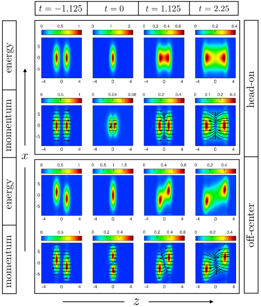
Figure 1: The rescaled energy density $\langle\widehat{T}^{00}\rangle$ and rescaled momentum density $|\langle T^{0i}\rangle|$, for head-on and off-center collisions at four different times. Streamlines in the plots of the momentum density denote the direction of the momentum density. At the initial time $t=-1.125$ the “protons” are at $z=\pm 1.125$. The non-zero impact parameter $\bm{b}=3\hat{x}$ is apparent in the off-center collision. The shocks move in the $\pm z$ direction at the speed of light and collide at $t=z=0$. After the collision the remnants of the initial shocks, which remain close to the light cone $z=\pm t$, are significantly attenuated in amplitude with the extracted energy deposited inside the light cone. Note the appearance of transverse flow at positive times for both impact parameters.

We shall employ the single shock energy density given in Eq. (1) in the Introduction. This means

$$H_{\pm}(\bm{x}_{\perp},z_{\mp})=\mu^{3}\exp\left[-{\textstyle\frac{1}{2}}(\bm{x}_{\perp}\mp{\textstyle\frac{\bm{b}}{2}})^{2}/\sigma^{2}\right]\delta_{w}(z_{\mp}).$$ (20)

For the smeared $\delta$ function we choose a Gaussian

$$\delta_{w}(z)=\frac{1}{\sqrt{2\pi w^{2}}}e^{-\frac{1}{2}z^{2}/w^{2}},$$ (21)

with width $\mu w=0.375$. Note that evolution inside the future light cone of planar shock collisions with width $\mu w=0.375$ well approximates that of the $\delta$ function limit [17]. The shock parameters we employ are given in Eq. (3) in the Introduction.

At early times, $t\ll-w$, the profiles $H_{\pm}$ have negligible overlap and the precollision geometry can be constructed from (16) by replacing the last term with the sum of corresponding terms from left and right moving shocks. The resulting metric satisfies Einstein’s equations, at early times, up to exponentially small errors.

To evolve the precollision geometry forward in time we use the characteristic formulation of gravitational dynamics in asymptotically AdS spacetimes. Here we simply outline the salient details of the characteristic formulation in asymptotically AdS spacetime. For details we refer the reader to [26]. Our metric ansatz reads

$$ds^{2}=r^{2}\,g_{\mu\nu}(x,r)\,dx^{\mu}dx^{\nu}+2\,dr\,dt\,,$$ (22)

with Greek indices denoting spacetime boundary coordinates, $x^{\mu}=(t,x,y,z)$. Near the boundary, $g_{\mu\nu}=\eta_{\mu\nu}+g_{\mu\nu}^{(4)}/r^{4}+O(1/r^{5})$. The subleading coefficients $g^{(4)}_{\mu\nu}$ determine the SYM stress tensor [25]

$$\langle T^{\mu\nu}\rangle=\frac{N_{\rm c}^{2}}{2\pi^{2}}\left[g_{\mu\nu}^{(4)}+\tfrac{1}{4}\,\eta_{\mu\nu}\,g_{00}^{(4)}\right].$$ (23)

An important practical matter in numerical relativity is determining the computational domain and excising singularities behind the event horizon. To excise singularities, we look for the position of an apparent horizon, which if it exists must lie behind an event horizon, and stop numerical evolution at its location. Note that the metric ansatz (22) is invariant under the residual diffeomorphism

$$r\to r+\lambda(t,\bm{x}),$$ (24)

for arbitrary $\lambda$. If the apparent horizon has planar topology and lies at say $r=r_{h}(t,\bm{x})$, then we may use this residual diffeomorphism invariance to set the apparent horizon to be at $r=1$ by choosing $\lambda=-1+r_{h}$. Let $\nabla$ be the covariant derivative under the spatial metric $g_{ij}$. Fixing the apparent horizon to be at constant $r$, at the horizon the metric must satisfy [26]

$$\left(\partial_{t}-{\textstyle\frac{1}{2}}g_{00}\partial_{r}\right)[\det g_{ij}]^{1/6}+{\textstyle\frac{1}{2}}(\partial_{r}[\det g_{ij}]^{1/6})g^{ij}g_{0i}g_{0j}-{\textstyle\frac{1}{3}}[\det g_{ij}]^{1/6}g^{ij}\nabla_{i}g_{0j}=0.$$ (25)

We note that Eq. (25) is a constraint on initial data: if (25) is satisfied at any fixed time and appropriate boundary conditions are enforced, then Einstein’s equations guarantee (25) remains satisfied at future times. See [26] for more details. Hence, we only need to enforce (25) on initial data. For given initial data we compute the LHS of (25) at $r=1$ and search for a radial shift $\lambda$ such that (25) is satisfied to some chosen accuracy. The shift $\lambda$ is computed using Newton’s method. In our numerical simulations we demand that the norm of the LHS of (25) is $5\times 10^{-3}$ or smaller.

To generate initial data for our characteristic evolution, we numerically transform the precollision metric in Fefferman-Graham coordinates to the metric ansatz (22). We begin time evolution at $t=-1.5$. For both head-on and off-center initial data we find an apparent horizon at time $t=-1.5$ — before the collision on the boundary. Since the apparent horizon must lie inside an event horizon, this means that there is an event horizon even before the collision takes place on the boundary. Why must an event horizon exist before the collision? Empty AdS contains a cosmological horizon, which is simply the Poincare horizon. It takes a light ray an infinite amount of (boundary) time to travel from the Poincare horizon to any bulk point in the geometry. This means that if a planar topology event horizon exists at any time — say after the collision — then it must have also existed at all times in the past and coincided with the Poincare horizon at $t=-\infty$. Similar conclusions were reached within the context of a quench studied in [27].

For numerical evolution we periodically compactly spatial directions with transverse size $L_{x}=L_{y}=18$ and longitudinal size $L_{z}=9$ and and evolve from $t=-1.5$ to $t=2.5$. For the head-on collision, evolution is performed using a spectral grid of size $N_{x}=N_{y}=39$, $N_{z}=155$ and $N_{r}=48$ while for the off-center collision we increase the number of transverse points to $N_{x}=N_{y}=45.$ To monitor the convergence of our numerical solution, we monitor violations of the horizon fixing condition (25). Since in the continuum limit (25) is an initial value constraint, violations of (25) after the initialization time $t=-1.5$ provide a simple measure of the degree in which our numerics are converging to the continuum limit. For both head-on and off-center collisions violations of (25) are $5\times 10^{-3}$ or smaller at all times, which is the same size of the allowed violations of (25) at the initialization time. The fact that (25) remains satisfied after the initialization time provides a nontrivial check of the convergence of our numerics.

4 Results

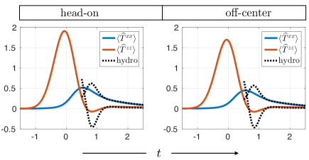
Figure 2: Rescaled stress tensor components $\langle\widehat{T}^{xx}\rangle$ and $\langle\widehat{T}^{zz}\rangle$ at the spatial origin, $x=y=z=0$, as a function of time for head-on and off-center collisions. Dashed lines denote the hydrodynamic approximation (6). Note that the stress in the different collisions are nearly identical. Around $t=0$ the systems are highly anisotropic and far from equilibrium. Nevertheless, at this point in space, the systems begins to evolve hydrodynamically at $t=t_{\rm hydro}\approx 1.2$. Note that the large pressure anisotropy persists during the hydrodynamic evolution.

Define the rescaled stress

$$\langle\widehat{T}^{\mu\nu}\rangle\equiv\frac{2\pi^{2}}{N_{\rm c}^{2}}\langle T^{\mu\nu}\rangle.$$ (26)

In Fig. 1 we plot the rescaled energy density $\langle\widehat{T}^{00}\rangle$ and the rescaled momentum density $\langle\widehat{T}^{0i}\rangle$ in the plane $y=0$ for head-on and off-center collisions at several values of time. The color scaling in the plots of $\langle\widehat{T}^{0i}\rangle$ denotes the magnitude of the momentum density $|\langle\widehat{T}^{0i}\rangle|$, while the streamlines indicate the direction of $\langle\widehat{T}^{0i}\rangle$. At time $t=-1.125$ the systems consist of two separated “protons” centered on $z=\pm 1.125$, $x=0$ for the head-on collision and $z=\pm 1.125$, $x=\mp\frac{b}{2}$ for the off-center collision. In both collisions the “protons” move towards each other at the speed of light and collide at $t=z=0$. Note that at $t=0$ the momentum density of the head-on collision nearly cancels out. Indeed, at $t=0$ the energy and momentum densities for both collisions are at the order 10% level just the linear superposition of that of the incoming “protons.” This indicates that nonlinear interactions haven’t yet modified the stress. Similar observations were made within the context of planar shock collisions in [16]. Nevertheless, at subsequent times we see that the collisions dramatically alter the outgoing state. For both collisions the amplitude of the energy and momentum densities near the forward light cone have decreased by order 50% relative to the past light cone, with the lost energy being deposited inside the forward light cone. Moreover, after $t=0$ we see the presence of transverse flow for both impact parameters. As we demonstrate below, the evolution of the postcollision debris for both impact parameters is well described by viscous hydrodynamics.

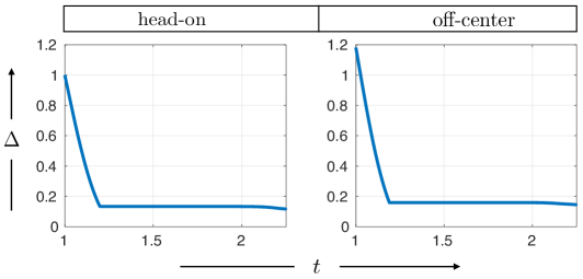
Figure 3: The hydrodynamic residual $\Delta$ at at the spatial origin, $x=y=z=0$, as a function of time for head-on and off-center collisions. Note that $\Delta$ need not be differentiable due to the max and matrix norm in its definition (15). Regions with $\Delta\ll 1$ have hydrodynamized. Prior to $t=t_{\rm hydro}\approx 1.2$, the residual is large and hydrodynamics is not a good description of the evolution. However, as $t\to t_{\rm hydro}$ the residual dramatically decreases. Thereafter, $\Delta$ continues to decrease but at a much slower rate. The rapid decay of $\Delta$ prior to $t=t_{\rm hydro}$ reflects the rapid decay of nonhydrodynamic modes in the far-from-equilibrium state created by the collisions.

In Fig. 2 we plot $\langle\widehat{T}^{xx}\rangle$ and $\langle\widehat{T}^{zz}\rangle$ and the hydrodynamic approximation $\widehat{T}^{xx}_{\rm hydro}$ and $\widehat{T}^{zz}_{\rm hydro}$ at the origin $\bm{x}=0$ for both impact parameters. At this point the stress tensor is diagonal, the flow velocity $\bm{u}=0$, and $\langle\widehat{T}^{xx}\rangle$ and $\langle\widehat{T}^{zz}\rangle$ are simply the pressures in the $x$ and $z$ directions. As shown in the figure, the pressures start off at zero before the collision. Note that the pressures are remarkably similar for both collisions. Evidently, the finite impact parameter employed here has little effect on the pressures at the origin. During the collisions the pressures increase dramatically, reflecting a system which is highly anisotropic and far from equilibrium. Nevertheless, after time

$$t=t_{\rm hydro}\approx 1.2,$$ (27)

the system has hydrodynamized at the origin and the evolution of the pressures for both impact parameters is well described by the hydrodynamic constitutive relations. Remarkably, at this time $\langle\widehat{T}^{xx}\rangle$ is order 10 times greater than $\langle\widehat{T}^{zz}\rangle$.

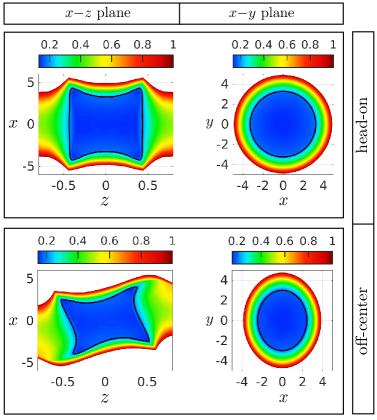
Figure 4: The hydrodynamic residual $\Delta$ in the $x{-}z$ and $x{-}y$ planes at time $t=1.25\,t_{\rm hydro}=1.5$ for both head-on and off-center collisions. Regions with $\Delta\ll 1$ have hydrodynamized. Note that we have restricted the plot to $\Delta<1$ in order to highlight the hydrodynamic behavior. The black curve in the plots is the surface $\Delta=0.2$. For both impact parameters there is a crisply defined region — whose boundary is well approximated by the $\Delta=0.2$ surface — where $\Delta\ll 1$. We identify the matter in the interior of the $\Delta=0.2$ surface as a droplet of liquid. Outside the $\Delta=0.2$ surface $\Delta$ rapidly increases, indicating the presence of nonhydrodynamic modes on the surface of the droplet. Note the irregularity in the off-center collision droplet shape in the $x{-}z$ plane is due to nonhydrodynamic modes and not fluid rotation in the $x{-}z$ plane. For the head-on collision the $\Delta=0.2$ surface is circular in the $x{-}y$ plane. In contrast, for the off-center collision the $\Delta=0.2$ surface is elliptical in the $x{-}y$ plane, with the the short axis of the ellipse oriented in the same direction as the impact parameter $\bm{b}=3\hat{x}$. Nevertheless, for both collisions the transverse radius of the $\Delta=0.2$ surface is roughly the same and equal to $R\sim 3$, which is just the radius $\sigma$ of our “protons.”

In Fig. 3 we plot the hydrodynamic residual $\Delta$ at $\bm{x}=0$ for both impact parameters. We see from the figure that $\Delta$ is large at times $t<t_{\rm hydro}$. However, as $t\to t_{\rm hydro}$ the residual $\Delta$ rapidly decays to $\Delta\lesssim 0.2$. After $t=t_{\rm hydro}$ the residual continues to decay, but at a much slower rate than before $t=t_{\rm hydro}$. The rapid decay of $\Delta$ prior to $t=t_{\rm hydro}$ indicates the rapid decay of nonhydrodynamic modes.

Over what region of space has the system hydrodynamized? To study the spatial domain of applicability of hydrodynamics, in Fig. 4 we plot $\Delta$ in the $x{-}z$ and $x{-}y$ planes at time $t=1.25\,t_{\rm hydro}=1.5$ for both head-on and off-center collisions. In order to highlight the hydrodynamic behavior, we omit regions where $\Delta>1$. For both collisions we see a region where $\Delta\ll 1$. In this region the stress has hydrodynamized and correspondingly, we identify the matter in the interior as a droplet of liquid. Also included in the figure is the surface $\Delta=0.2$, shown as the solid curve. For both collisions $\Delta$ increases dramatically outside the $\Delta=0.2$ surface, indicating the presence of nonhydrodynamic modes. In what follows we shall use the $\Delta=0.2$ surface to define the surface of our droplet of liquid.

Note the irregularity in the off-center collision droplet shape in the $x{-}z$ plane is due to nonhydrodynamic modes and not fluid rotation in the $x{-}z$ plane. Indeed, in the interior of the droplet the vorticity is small with $||\Omega^{\mu\nu}||\sim 0.1||\sigma^{\mu\nu}||$. Additionally, note the difference in droplet shape in the $x{-}y$ plane for head-on and off-center collisions. For the head-on collision droplet’s surface is circular in the $x{-}y$ plane. In contrast, for the off-center collision the droplet’s surface is elliptical in the $x{-}y$ plane, with the the short axis of the ellipse oriented in the same direction as the impact parameter $\bm{b}=3\hat{x}$. Nevertheless, for both collisions the transverse radius of the droplet is roughly the same and equal to $R\sim 3$, which is just the radius $\sigma$ of our “protons” employed in (3).

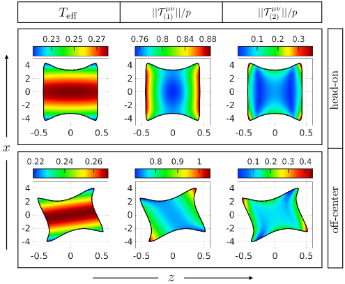
Figure 5: The effective temperature $T_{\rm eff}$ and the first and second order gradient norms $||\mathcal{T}_{(1)}^{\mu\nu}||$ and $||\mathcal{T}_{(2)}^{\mu\nu}||$ in units of the average pressure $p$ for head-on and off-center collisions. All plots are shown at time $t=1.25\,t_{\rm hydro}=1.5$ and are restricted to the domain inside the $\Delta=0.2$ surface shown in Fig. 4, which is also shown here as the solid curve. In this region hydrodynamics is a good approximation to the evolution of the stress. For both collisions the average effective temperature in the displayed region is $T_{\rm eff}\sim 0.25$. Inside the $\Delta=0.2$ surface $||\mathcal{T}_{(2)}^{\mu\nu}||\ll||\mathcal{T}_{(1)}^{\mu\nu}||$, meaning second order gradient corrections are negligible. Note however, that near the surface of the droplet, where nonhydrodynamic modes are excited, $||\mathcal{T}_{(2)}^{\mu\nu}||$ begins to become comparable to $||\mathcal{T}_{(1)}^{\mu\nu}||$.

In Figs. 5-7 we restrict our attention to time $t=1.25\,t_{\rm hydro}=1.5$ and to the region inside the droplet of fluid. We explain the coloring of the different plots below. In the left column of Fig. 5 we show the effective temperature $T_{\rm eff}$, defined in Eq. (12). From the figure it is evident that the average value of the temperature inside the droplet is $T_{\rm eff}\sim 0.25$ for both collisions. We therefore obtain the dimensionless measure of the transverse size of the droplet,

$$RT_{\rm eff}\sim 1.$$ (28)

Similar conclusions were reached in [18], where a holographic model of proton-nucleus collisions was studied. Additionally, note

$$t_{\rm hydro}T_{\rm eff}\sim 0.3,$$ (29)

indicating rapid hydrodynamization. Similar hydrodynamization times were observed in [18, 16, 28, 29]. We therefore conclude that hydrodynamic evolution applies even when both the system size and time after the collision are on the order of microscopic scale $1/T_{\rm eff}$.

In the middle and right columns of Figs. 5 we plot the size of first and second order gradient corrections to the hydrodynamic constitutive relations, $||\mathcal{T}^{\mu\nu}_{(1)}||$ and $||\mathcal{T}^{\mu\nu}_{(2)}||$, normalized by the average pressure $p$. In the interior of the droplet $||\mathcal{T}^{\mu\nu}_{(2)}||$ is nearly an order of magnitude smaller than $||\mathcal{T}^{\mu\nu}_{(1)}||$ for both impact parameters, meaning that second order gradient corrections are negligible.

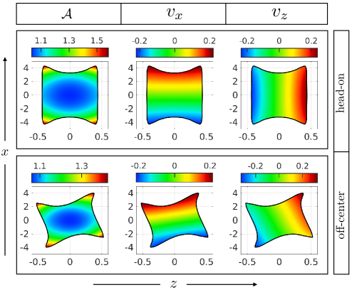
Figure 6: The anisotropy $\mathcal{A}$ and the transverse and longitudinal components of the fluid 3-velocity $\bm{v}\equiv\bm{u}/u^{0}$ for head-on and off-center collisions. All plots are shown at time $t=1.25\,t_{\rm hydro}=1.5$ and are restricted to the domain inside the $\Delta=0.2$ contour shown in Fig. 4, which is also shown here as the solid curve. In this region hydrodynamics is a good approximation of the evolution of the stress. In the limit of ideal hydrodynamics the anisotropy vanishes. The order 1 anisotropy observed here for both collisions reflects the fact that there are large gradients in the system. Likewise, for both collisions we see that $v_{x}$ and $v_{z}$ are similar in magnitude. The large transverse velocity is also a signature of large gradients.

5 Discussion

Given that $1/T_{\rm eff}$ is the salient microscopic scale in strongly coupled plasma — akin to the mean free path at weak coupling — it is remarkable that hydrodynamics can describe the evolution of systems as small at $1/T_{\rm eff}$. By setting the “proton” radius equal to the actual proton radius, $\sigma\sim 1$ fm, and using $N_{\rm c}=3$ colors, the single shock energy (2) is $\sim 20$ GeV. Likewise, the effective temperature of the produced plasma is $T_{\rm eff}\sim 200$ MeV. Given that collisions at RHIC and the LHC have higher energies and temperatures, it is natural to expect $RT_{\rm eff}$ to be larger in RHIC and LHC collisions than the simulated collision presented here. We therefore conclude that droplets of liquid the size of the proton need not be thought of as unnaturally small. Evidently, there are theories — namely strongly coupled SYM — which enjoy hydrodynamic evolution in even smaller systems.

While hydrodynamics is a good description of the evolution of our collision, it should be noted that the produced hydrodynamic flow has an extreme character to it. In particular, when the system size is on the order of the microscopic scale $1/T_{\rm eff}$, gradients must be large. To quantify the size of gradients we introduce the anisotropy function

$$\mathcal{A}\equiv\frac{{\rm max}(p_{(i)})-{\rm min}(p_{(i)})}{p},$$ (30)

where the pressures $p_{(i)}$ are determined by the eigenvalue equation (13) and again $p$ is the average pressure, $p=\frac{\epsilon}{3}={\rm avg}(p_{(i)})$. In ideal hydrodynamics, where all the pressures $p_{(i)}$ are equal, the anisotropy vanishes. It therefore follows that after the system has hydrodynamized, any nonzero anisotropy must be due to gradient corrections in the hydrodynamic constitutive relations (6). In the left column of Fig. 6 we plot $\mathcal{A}$ at time $t=1.25\,t_{\rm hydro}=1.5$ in the interior of the droplet. For both impact parameters $\mathcal{A}\sim 1$, with larger anisotropies near the droplet’s surface. Evidently, gradients are large and ideal hydrodynamics is not a good approximation. This is also evident in the pressures displayed in Fig. 2, where the transverse and longitudinal pressures differ by a factor of 5 to 10. Moreover, as shown in Fig. 5, $||\mathcal{T}^{\mu\nu}_{(1)}||\sim p$, so the first order gradient correction $\mathcal{T}^{\mu\nu}_{(1)}$ is comparable to the ideal hydrodynamic stress. However, despite the presence of large gradients, the above observed large anisotropy must be almost entirely due to the first order gradient correction $\mathcal{T}^{\mu\nu}_{(1)}$ alone, since $||\mathcal{T}^{\mu\nu}_{(2)}||$ is nearly an order of magnitude smaller than $||\mathcal{T}^{\mu\nu}_{(1)}||$ inside the droplet of fluid. This means that viscous hydrodynamics alone is sufficient to capture the observed large anisotropies and evolution of the system.

It is remarkable that the second order gradient correction $\mathcal{T}^{\mu\nu}_{(2)}$ is negligible even when gradients are large enough to produce an order 1 anisotropy. It is also remarkable that the presence of large gradients does not substantially excite nonhydrodynamic modes (e.g. nonhydrodynamic quasinormal modes). In an infinite box of liquid, nonhydrodynamic modes decay over a timescale of order $1/T_{\rm eff}$. Evidently, in the interior of the small droplet studied here, the rate of decay of nonhydrodynamic modes is stronger than the rate in which they are excited.

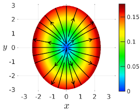
Figure 7: The fluid 3-velocity $\bm{v}$ in the $x{-}y$ plane at time $t=1.25t_{\rm hydro}$. The coloring denotes the magnitude of the 3-velocity while the streamlines denote its direction. Note that we have restricted the plot to the interior of the $\Delta=0.2$ surface.

We now turn to the nature of the produced hydrodynamic flow. Also shown in Fig. 6 are the transverse and longitudinal components of the fluid 3-velocity, $\bm{v}\equiv\bm{u}/u^{0}$, at time $t=1.25\,t_{\rm hydro}$ for both head-on and off-center collisions. $v_{x}$ and $v_{z}$ are similar in magnitude for both impact parameters. Given that the transverse velocity starts from zero and is driven by transverse gradients, the rapid development of transverse flow observed here must reflect the presence of large transverse gradients. In Fig. 7 we plot the 3-velocity in the $x{-}y$ plane at time $t=1.25\,t_{\rm hydro}$ in the interior of the droplet produced in the off-center collision. The coloring in the plot denotes the magnitude of the fluid 3-velocity while the streamlines denote its direction. The fluid velocity is not radial, which is natural given the finite impact parameter and the elliptical shape of the droplet in the $x{-}y$ plane. However, the flow of momentum is nearly radial. To quantify this, define the Fourier coefficient $c_{n}\equiv\int d^{3}x\langle T^{0i}\rangle\hat{\rho}^{i}\cos n\phi$ where $\hat{\rho}=\cos\phi\hat{x}+\sin\phi\hat{y}$ is the radial unit vector with $\phi$ the azimuthal angle. Deviations in radial flow are encoded in $c_{2}$. However, at time $t=1.25\,t_{\rm hydro}$, the coefficient $c_{2}$ is only 1% of $c_{0}$, indicating small deviations from radial momentum flow. It would be interesting to see how $c_{2}$ grows as time progresses. It would also be interesting to see how $c_{2}$ is affected by different choices of shock profiles. Indeed, off-center collisions of Gaussian shock profiles with large transverse width $\sigma$ generate purely radial flow [19], since the overlap of two off-center Gaussians is still a Gaussian and thus rotationally invariant about the $z$ axis.

Let us now ask how the droplet of fluid produced in the collision further evolves at later times. In conformal SYM the droplet must expand forever with size $R\sim t$. This is very different from a confining theory, where the droplet cannot expand indefinitely. Likewise, as the droplet expands it must cool. Its easy to reason from energy conservation that the temperature must decrease slower than $1/t$, meaning that $RT_{\rm eff}\to\infty$ as $t\to\infty$, so hydrodynamics becomes a better and better description of the evolution. We expect the surface of the droplet to become smoother and smoother as time progresses. Likewise, we expect nonhydrodynamic modes near the surface of the droplet to continue to decay with the fraction of energy behaving hydrodynamically approaching 100% as $t\to\infty$. Indeed, such behavior was observed within the context of planar shock collisions [17], where nonhydrodynamic modes near the light cone decayed, with the lost energy transported inside the light cone where it hydrodynamizes.

It would be interesting to push our analysis further. How big are the smallest drops of liquid? Clearly $RT_{\rm eff}$ cannot be made arbitrarily small since the hydrodynamic gradient expansion (6) breaks down when $RT_{\rm eff}\ll 1$. Moreover, in the gravitational description there likely exists a critical energy $E_{c}$ (or alternatively a critical impact parameter $b_{c}$ [30]) below (above) which no black hole is formed and which for $E=E_{c}+0^{+}$(or $b=b_{c}+0^{-})$ critical gravitational collapse occurs [31]. The absence of a black hole when $E<E_{c}$ (or $b>b_{c}$) means that in the dual field theory the collisional debris will not evolve hydrodynamically at any future time. Clearly it would be interesting to look for criticality and the associated signatures of hydrodynamics turning off.

It would also be of great interest to study collisions in confining theories. Aside from being more realistic, collisions in confining theories have the added feature that the produced droplet — a plasma ball — cannot expand indefinitely. As the system cools it must eventually reach the confinement/deconfinement transition and freeze into a gas of hadrons. In the large $N_{\rm c}$ limit freezeout is suppressed and plasma balls are metastable with a lifetime of order $N_{\rm c}^{2}$ [32]. At $N_{\rm c}=\infty$, plasma balls must eventually equilibrate and become static due to internal frictional forces. Therefore, in a large $N_{\rm c}$ confining theory the question of how big are the smallest drops of quark-gluon plasma is tantamount to how big are the smallest plasma balls. An illuminating warmup problem is that of SYM on a three sphere of radius $R$. In the large $N_{\rm c}$ limit the theory becomes confining [33, 34, 35]. Therefore, instead of studying plasma balls produced in a collision, one can study plasma confined to the three sphere and analyze the plasma’s behavior as the radius of the sphere is changed.

The dual gravitational description of SYM on a three sphere is that of gravity in global AdS₅$\times S^{5}$. At strong coupling, and in the canonical ensemble, the deconfinement temperature $T_{c}$ is

$$RT_{c}=\frac{3}{2\pi}\approx 0.48,$$ (31)

with the deconfinement transition manifesting itself in the gravity description as the Hawking-Page phase transition [33]. Above the deconfinement transition the dual geometry contains a black hole, the boundary energy density is order $N_{\rm c}^{2}$, and the boundary state is that of a quark-gluon plasma with hydrodynamic evolution. Below the transition the dual geometry is just thermal AdS and the boundary state has order $N_{\rm c}^{0}$ energy and does not admit a hydrodynamic description. Hence in the canonical ensemble of SYM living on a three sphere, the answer to the question of how big are the smallest drops of quark-gluon plasma is given by (31).

The situation is less clear in the microcannonical ensemble. In this case the dual black hole geometry experiences a Gregory-Laflamme instability [36] on the $S^{5}$ [37, 38, 39]. The instability sets in at

$$RT_{\rm eff}\approx 0.50.$$ (32)

It is unknown what the final state of the Gregory-Laflamme instability is. One possibility is that there do not exist stable black hole solutions below (32). In this case the instability could go on indefinitely, perhaps generating structures on the order of the Planck scale where quantum effects will be important. Another possibility is that there exists equilibrium black holes with broken rotational invariance on the $S^{5}$. In this case the final state of the Gregory-Laflamme instability would asymptote to this solution. In either case, it seems likely that the onset of the Gregory-Laflamme instability destroys hydrodynamic evolution in the dual field theory. It therefore seems that in either ensemble, the smallest drops of quark-gluon plasma in the confining phase of SYM have size $RT_{\rm eff}\approx 1/2.$

6 Acknowledgments

This work is supported by the Fundamental Laws Initiative at Harvard. I thank Krishna Rajagopal, Andy Strominger and Larry Yaffe for useful discussions.

References

- [1] CMS collaboration, S. Chatrchyan et al., Multiplicity and transverse momentum dependence of two- and four-particle correlations in pPb and PbPb collisions, Phys.Lett. B724 (2013) 213–240, [1305.0609].
- [2] ALICE collaboration, B. Abelev et al., Long-range angular correlations on the near and away side in -Pb collisions at TeV, Phys.Lett. B719 (2013) 29–41, [1212.2001].
- [3] ATLAS collaboration, G. Aad et al., Observation of Associated Near-Side and Away-Side Long-Range Correlations in =5.02??TeV Proton-Lead Collisions with the ATLAS Detector, Phys.Rev.Lett. 110 (2013) 182302, [1212.5198].
- [4] PHENIX collaboration, A. Adare et al., Quadrupole Anisotropy in Dihadron Azimuthal Correlations in Central Au Collisions at =200 GeV, Phys.Rev.Lett. 111 (2013) 212301, [1303.1794].
- [5] PHENIX collaboration, A. Adare et al., Measurements of elliptic and triangular flow in high-multiplicity 3HeAu collisions at GeV, Phys. Rev. Lett. 115 (2015) 142301, [1507.06273].
- [6] ATLAS collaboration, G. Aad et al., Observation of long-range elliptic anisotropies in 13 and 2.76 TeV collisions with the ATLAS detector, 1509.04776.
- [7] P. Bozek, Collective flow in p-Pb and d-Pd collisions at TeV energies, Phys.Rev. C85 (2012) 014911, [1112.0915].
- [8] P. Bozek and W. Broniowski, Correlations from hydrodynamic flow in p-Pb collisions, Phys.Lett. B718 (2013) 1557–1561, [1211.0845].
- [9] A. Bzdak, B. Schenke, P. Tribedy and R. Venugopalan, Initial state geometry and the role of hydrodynamics in proton-proton, proton-nucleus and deuteron-nucleus collisions, Phys.Rev. C87 (2013) 064906, [1304.3403].
- [10] B. Schenke and R. Venugopalan, Eccentric protons? Sensitivity of flow to system size and shape in p+p, p+Pb and Pb+Pb collisions, Phys. Rev. Lett. 113 (2014) 102301, [1405.3605].
- [11] M. Habich, G. A. Miller, P. Romatschke and W. Xiang, A Hydrodynamic Study of pp Collisions at TeV, 1512.05354.
- [12] J. M. Maldacena, The Large N limit of superconformal field theories and supergravity, Int. J. Theor. Phys. 38 (1999) 1113–1133, [hep-th/9711200].
- [13] D. Grumiller and P. Romatschke, On the collision of two shock waves in AdS(5), JHEP 08 (2008) 027, [0803.3226].
- [14] J. L. Albacete, Y. V. Kovchegov and A. Taliotis, Modeling Heavy Ion Collisions in AdS/CFT, JHEP 07 (2008) 100, [0805.2927].
- [15] P. M. Chesler and L. G. Yaffe, Holography and colliding gravitational shock waves in asymptotically AdS5 spacetime, Phys. Rev. Lett. 106 (2011) 021601, [1011.3562].
- [16] J. Casalderrey-Solana, M. P. Heller, D. Mateos and W. van der Schee, From full stopping to transparency in a holographic model of heavy ion collisions, Phys. Rev. Lett. 111 (2013) 181601, [1305.4919].
- [17] P. M. Chesler, N. Kilbertus and W. van der Schee, Universal hydrodynamic flow in holographic planar shock collisions, JHEP 11 (2015) 135, [1507.02548].
- [18] P. M. Chesler, Colliding shock waves and hydrodynamics in small systems, Phys. Rev. Lett. 115 (2015) 241602, [1506.02209].
- [19] P. M. Chesler and L. G. Yaffe, Holography and off-center collisions of localized shock waves, JHEP 10 (2015) 070, [1501.04644].
- [20] R. Baier, P. Romatschke, D. T. Son, A. O. Starinets and M. A. Stephanov, Relativistic viscous hydrodynamics, conformal invariance, and holography, JHEP 04 (2008) 100, [0712.2451].
- [21] P. Romatschke, New Developments in Relativistic Viscous Hydrodynamics, Int. J. Mod. Phys. E19 (2010) 1–53, [0902.3663].
- [22] S. Bhattacharyya, V. E. Hubeny, S. Minwalla and M. Rangamani, Nonlinear Fluid Dynamics from Gravity, JHEP 02 (2008) 045, [0712.2456].
- [23] G. Policastro, D. T. Son and A. O. Starinets, The Shear viscosity of strongly coupled N=4 supersymmetric Yang-Mills plasma, Phys. Rev. Lett. 87 (2001) 081601, [hep-th/0104066].
- [24] S. S. Gubser, S. S. Pufu and A. Yarom, Entropy production in collisions of gravitational shock waves and of heavy ions, Phys. Rev. D78 (2008) 066014, [0805.1551].
- [25] S. de Haro, S. N. Solodukhin and K. Skenderis, Holographic reconstruction of space-time and renormalization in the AdS / CFT correspondence, Commun. Math. Phys. 217 (2001) 595–622, [hep-th/0002230].
- [26] P. M. Chesler and L. G. Yaffe, Numerical solution of gravitational dynamics in asymptotically anti-de Sitter spacetimes, JHEP 07 (2014) 086, [1309.1439].
- [27] P. M. Chesler and L. G. Yaffe, Horizon formation and far-from-equilibrium isotropization in supersymmetric Yang-Mills plasma, Phys. Rev. Lett. 102 (2009) 211601, [0812.2053].
- [28] M. P. Heller, R. A. Janik and P. Witaszczyk, Hydrodynamic Gradient Expansion in Gauge Theory Plasmas, Phys. Rev. Lett. 110 (2013) 211602, [1302.0697].
- [29] P. M. Chesler and L. G. Yaffe, Boost invariant flow, black hole formation, and far-from-equilibrium dynamics in N = 4 supersymmetric Yang-Mills theory, Phys. Rev. D82 (2010) 026006, [0906.4426].
- [30] S. Lin and E. Shuryak, Grazing Collisions of Gravitational Shock Waves and Entropy Production in Heavy Ion Collision, Phys. Rev. D79 (2009) 124015, [0902.1508].
- [31] M. W. Choptuik, Universality and scaling in gravitational collapse of a massless scalar field, Phys.Rev.Lett. 70 (1993) 9–12.
- [32] O. Aharony, S. Minwalla and T. Wiseman, Plasma-balls in large N gauge theories and localized black holes, Class. Quant. Grav. 23 (2006) 2171–2210, [hep-th/0507219].
- [33] E. Witten, Anti-de Sitter space, thermal phase transition, and confinement in gauge theories, Adv. Theor. Math. Phys. 2 (1998) 505–532, [hep-th/9803131].
- [34] O. Aharony, J. Marsano, S. Minwalla, K. Papadodimas and M. Van Raamsdonk, The Hagedorn - deconfinement phase transition in weakly coupled large N gauge theories, Adv. Theor. Math. Phys. 8 (2004) 603–696, [hep-th/0310285].
- [35] O. Aharony, J. Marsano, S. Minwalla, K. Papadodimas and M. Van Raamsdonk, A First order deconfinement transition in large N Yang-Mills theory on a small S**3, Phys. Rev. D71 (2005) 125018, [hep-th/0502149].
- [36] R. Gregory and R. Laflamme, Black strings and p-branes are unstable, Phys. Rev. Lett. 70 (1993) 2837–2840, [hep-th/9301052].
- [37] V. E. Hubeny and M. Rangamani, Unstable horizons, JHEP 05 (2002) 027, [hep-th/0202189].
- [38] A. Buchel and L. Lehner, Small black holes in , Class. Quant. Grav. 32 (2015) 145003, [1502.01574].
- [39] O. J. C. Dias, J. E. Santos and B. Way, Lumpy AdS S5 black holes and black belts, JHEP 04 (2015) 060, [1501.06574].