YITP-16-1

Probing the Small-$x$ Gluon Tomography in Correlated Hard Diffractive Dijet Production in DIS

Abstract

We investigate the close connection between the quantum phase space Wigner distribution of small-$x$ gluons and the color dipole scattering amplitude, and propose to study it experimentally in the hard diffractive dijet production at the planned electron-ion collider. The angular correlation between the nucleon recoiled momentum and the dijet transverse momentum will probe the nontrivial correlation in the phase space Wigner distribution. This experimental study will not only provide us with three-dimensional tomographic pictures of gluons inside high energy proton, but also give a unique and interesting signal for the small-$x$ dynamics with QCD evolution effects.

Introduction. There have been strong interests in hadron physics community Boer:2011fh ; AbelleiraFernandez:2012cc ; Accardi:2012qut to explore the partonic structure of the nucleon, in particular, aiming at a tomography picture from which we can image the partons in three-dimensional fashion. This can provide fruitful and detailed information on the sub-atomic structure of the baryonic building blocks of the universe, and deepen our understanding of the strong interaction facts in constructing the fundamental particles. Among these tomography distributions, the so-called quantum phase space Wigner distributions Ji:2003ak ; Belitsky:2003nz of partons have been reckoned as the mother distributions of all, since they ingeniously encode all quantum information of how partons are distributed inside hadrons.

The key question now is to find experimental probes to measure these distributions. The goal of this paper is to pioneer this direction, by pointing out that we can have access to the gluon Wigner distributions at small-$x$. The proposed new observables will stimulate further developments from both experiment and theory sides for the planned electron-ion colliders (EIC). In general, it is believed that the parton Wigner distributions normally are not directly measurable in high energy scatterings. Due to the uncertainty principle, Wigner distributions, which are not positive definite, are only quasi-probabilistic. As we will demonstrate later in this Letter, one can use the diffractive dijet production (or more complicated processes), which has been a subject of study in the small-$x$ physics and the generalized parton distribution approach Nikolaev:1994cd ; Bartels:1996ne ; Bartels:1996tc ; Diehl:1996st ; Braun:2005rg ; Rezaeian:2012ji , to directly probe the Fourier transform of the gluon Wigner distribution at the EIC.

The phase space distributions Mueller:1999wm of quarks and gluons are often used in small-$x$ literatures, and they are believed to be possibly related to Wigner distributions Ji:2003ak , although the exact connection was not known. We will show that the gluon Wigner distributions at small-$x$ can be simplified and written as the Fourier transform of well-known impact parameter dependent dipole amplitudes, which helps us to build intimate connections to small-$x$ factorization framework developed in the last few decades. This will not only provide the motivation to pursue the gluon Wigner distributions in the future EIC, but also prompt further studies to investigate non-trivial correlations in the small-$x$ dipole scattering amplitude. The latter has become one of the most important elements of the phenomenological studies in heavy ion collisions and deep inelastic scatterings Gelis:2010nm ; Kovchegov:2012mbw .

One of the nontrivial phenomena is the angular correlation between the traverse momentum of the produced dijet and the recoiled momentum of the nucleon, which provides vital information on the gluon Wigner distributions. It is important to emphasize that this correlation can help us test and measure the unique feature of angular correlations between impact parameter and dipole size predicted by small-$x$ evolutions.

The rest of the paper is organized as follows. We first introduce the gluon Wigner distributions and take the small-$x$ limit, which can be connected to the dipole scattering amplitudes. We then explore the small-$x$ dynamics by invoking the analytical solution to the BFKL equation BFKLeq to show there exist nontrivial correlation in these gluon Wigner distributions. Last, we apply these results to demonstrate that we will be able to observe these novel correlations in the future EIC. Finally, we summarize our paper in the end.

Gluon Wigner Distributions at Small-$x$. The parton Wigner distributions are introduced to describe the quantum phase space distributions of partons inside the nucleon. They unify the two common languages of transverse momentum dependent and the generalized parton distributions in parton distributions framework.

We focus on the gluon Wigner distributions. Similar study can be done for the quark part. The gluon Wigner distributions are defined through the following matrix elements,

$$xW_{g}^{T}(x,\vec{q}_{\perp};\vec{b}_{\perp})=\int\frac{d\xi^{-}d^{2}\xi_{\perp}}{(2\pi)^{3}P^{+}}\int\frac{d^{2}\Delta_{\perp}}{(2\pi)^{2}}e^{-ixP^{+}\xi^{-}-iq_{\perp}\cdot\xi_{\perp}}\left\langle P+\frac{\Delta_{\perp}}{2}\left|F^{+i}\left(\vec{b}_{\perp}+\frac{\xi}{2}\right)F^{+i}\left(\vec{b}_{\perp}-\frac{\xi}{2}\right)\right|P-\frac{\Delta_{\perp}}{2}\right\rangle\,,$$ (1)

where $F^{\mu\nu}$ represents the field strength tensor, $x$ and $q_{\perp}$ for the longitudinal momentum fraction and the transverse momentum for the gluon, $\vec{b}_{\perp}$ for the coordinate space variable. The above Wigner distributions not only provide us with the momentum distribution of the corresponding parton, but also give the average location of that parton w.r.t. the center of target hadron. In the following, we will work in the small-$x$ limit where we can simplify the above expression and relate it to the dipole scattering amplitudes commonly used in the small-$x$ factorization approach. The Fourier transform of the Wigner distribution w.r.t. the impact parameter $b_{\perp}$ is also referred as the generalized transverse momentum dependent (GTMD) gluon distribution Meissner:2009ww ; Lorce:2013pza .

In Ref. Dominguez:2010xd ; Dominguez:2011wm , it has been demonstrated that TMD gluon distributions are related to small-$x$ unintegrated gluon distributions. The Weizsäcker-Williams (WW) and the dipole gluon distribution used in small-$x$ formalism correspond to two gauge invariant but topologically different operator definitions. In order to pursue deeper connections between Wigner distributions and small-$x$ impact parameter dependent gluon distributions, we first use the dipole gluon distribution as an example, and we will comment on the case of the WW gluon distribution in the end. Following the convention in Ref. Bomhof:2006dp , we write down the GTMD dipole gluon distribution as

$$xG_{\textrm{DP}}(x,q_{\perp},\Delta_{\perp})=2\int\frac{\text{d}\xi^{-}\text{d}^{2}\xi_{\perp}e^{-iq_{\perp}\cdot\xi_{\perp}-ixP^{+}\xi^{-}}}{\left(2\pi\right)^{3}P^{+}}\left\langle P+\frac{\Delta_{\perp}}{2}\left|\text{Tr}\left[F^{+i}\left(\xi/2\right)\mathcal{U}^{\left[-\right]\dagger}F^{+i}\left(-\xi/2\right)\mathcal{U}^{\left[+\right]}\right]\right|P-\frac{\Delta_{\perp}}{2}\right\rangle\,,$$ (2)

where $\mathcal{U}^{[\pm]}$ are the future/past-pointing U-shaped Wilson lines which make the operator gauge invariant. Its Fourier transform $\int\frac{d^{2}\Delta_{\perp}}{(2\pi)^{2}}e^{i\Delta_{\perp}\cdot b_{\perp}}xG_{\textrm{DP}}(x,q_{\perp},\Delta_{\perp})$ can be identified as the Wigner distribution $xW_{g}^{T}(x,q_{\perp},b_{\perp})$. Following similar derivation used in Ref Bomhof:2006dp ; Belitsky:2002sm ; Dominguez:2011wm in the small-$x$ limit, one can show that Eq. (2) reduces to

$$xG_{\textrm{DP}}(x,q_{\perp},\Delta_{\perp})=\frac{2N_{c}}{\alpha_{s}}\int\frac{d^{2}R_{\perp}d^{2}R_{\perp}^{\prime}}{(2\pi)^{4}}e^{iq_{\perp}\cdot\left(R_{\perp}-R_{\perp}^{\prime}\right)+i\frac{\Delta_{\perp}}{2}\cdot(R_{\perp}+R_{\perp}^{\prime})}\left(\nabla_{R_{\perp}}\cdot\nabla_{R_{\perp}^{\prime}}\right)\frac{1}{N_{c}}\left\langle\text{Tr}\left[U\left(R_{\perp}\right)U^{\dagger}\left(R_{\perp}^{\prime}\right)\right]\right\rangle_{x}\,,$$ (3)

where we can recognize the impact parameter dependent dipole amplitude. Let us define its double Fourier transform

$$\frac{1}{N_{c}}\text{Tr}\left[U\left(b_{\perp}+\frac{r_{\perp}}{2}\right)U^{\dagger}\left(b_{\perp}-\frac{r_{\perp}}{2}\right)\right]\equiv\int d^{2}q_{\perp}d^{2}\Delta_{\perp}e^{-iq_{\perp}\cdot r_{\perp}-i\Delta_{\perp}\cdot b_{\perp}}\mathcal{F}_{x}(q_{\perp},\Delta_{\perp})\,.$$ (4)

Then we can succinctly write $xG_{\textrm{DP}}(x,q_{\perp},\Delta_{\perp})=(q_{\perp}^{2}-\Delta_{\perp}^{2}/4)\frac{2N_{c}}{\alpha_{s}}\mathcal{F}_{x}(q_{\perp},\Delta_{\perp})$. Setting $r_{\perp}=0$ in the above expression, we obtain the normalization condition for $\mathcal{F}_{x}(q_{\perp},\Delta_{\perp})$ as $\int d^{2}q_{\perp}d^{2}\Delta_{\perp}e^{-i\Delta_{\perp}\cdot b_{\perp}}\mathcal{F}_{x}(q_{\perp},\Delta_{\perp})=1$.

Gluon Tomography Induced by Small-$x$ Dynamics. In the small-$x$ literature, the dipole scattering amplitudes have been widely used to describe the relevant processes such as the inclusive DIS, inclusive hadron production in $pA$ collisions. In these calculations, the dipole amplitude is averaged over the azimuthal angle of impact parameter $\vec{b}_{\perp}$. This is because most of the observables discussed in phenomenology so far are not sensitive to the $\vec{b}_{\perp}$-dependence. On the other hand, there have been theoretical investigations Lipatov:1985uk ; Navelet:1997tx ; Navelet:1997xn on the correlation between $\vec{b}_{\perp}$ and the dipole size $\vec{r}_{\perp}$, which eventually leads to nontrivial correlations between $\vec{b}_{\perp}$ and the transverse momentum $\vec{q}_{\perp}$ in the gluonic Wigner distributions. In the following, as a simple example, we illustrate how these correlations are generated at small-$x$ in the BFKL approximation. This provides an intuitive picture of small-$x$ gluon distributions in the nucleon.

Let us consider the dipole scattering amplitude off a dipole $x_{\perp}$ (quark at $\vec{x}_{\perp}/2$, antiquark at $-\vec{x}_{\perp}/2$) evolved up to rapidity $Y=\ln 1/x$. Define the dipole T-matrix in impact parameter space as $\frac{1}{N_{c}}\left\langle{\rm tr}\,U\left(b_{\perp}+\frac{r_{\perp}}{2}\right)U^{\dagger}\left(b_{\perp}-\frac{r_{\perp}}{2}\right)\right\rangle_{x}=1-T(r_{\perp},b_{\perp},Y)$. In the BFKL approximation, $T$ is given by Lipatov:1985uk ; Navelet:1997tx ; Navelet:1997xn

$$T(r_{\perp},b_{\perp},Y) = 2\pi\alpha_{s}^{2}\sum_{n}\int\frac{d\nu}{(2\pi)^{3}}\frac{(1+(-1)^{n})\left(\nu^{2}+\frac{n^{2}}{4}\right)}{\left(\nu^{2}+\left(\frac{n-1}{2}\right)^{2}\right)\left(\nu^{2}+\left(\frac{n+1}{2}\right)^{2}\right)}e^{\chi(n,\nu)Y}$$ (5)

$$\qquad\times\int d^{2}\omega_{\perp}E^{1-h,1-\bar{h}}(b_{\perp}+\frac{r_{\perp}}{2}-\omega_{\perp},b_{\perp}-\frac{r_{\perp}}{2}-\omega_{\perp})E^{h,\bar{h}}(\frac{x_{\perp}}{2}-\omega_{\perp},-\frac{x_{\perp}}{2}-\omega_{\perp})\,,$$

where $E^{h,\bar{h}}(a-\omega,b-\omega)=(-1)^{n}\left(\frac{z_{ab}}{z_{a\omega}z_{b\omega}}\right)^{h}\left(\frac{\bar{z}_{ab}}{\bar{z}_{a\omega}\bar{z}_{b\omega}}\right)^{\bar{h}}$ is the BFKL holomorphic eigenfunction with $h=\frac{1-n}{2}+i\nu$ and $\bar{h}=\frac{1+n}{2}+i\nu$. $\chi(n,\nu)\equiv\frac{2\alpha_{s}N_{c}}{\pi}\left[\psi(1)-\textrm{Re}\psi(\frac{|n|+1}{2}+i\nu)\right]$ is the BFKL characteristic function. In the high energy limit, the $n=0$ part of the solution gives the leading contribution. Using the saddle point approximation around $\nu=0$ and taking the limit $x_{\perp}\ll b_{\perp},r_{\perp}$, we can cast Eq. (5) into

$$T(r_{\perp},b_{\perp},Y)\approx\frac{\alpha_{s}^{2}|\rho|}{\sqrt{\pi}}\frac{\ln\frac{16}{|\rho|}}{\left(\frac{7}{2}\bar{\alpha}_{s}\zeta(3)Y\right)^{3/2}}\exp\left(4\bar{\alpha}_{s}Y\ln 2-\frac{\ln^{2}\frac{16}{|\rho|}}{14\bar{\alpha}_{s}\zeta(3)Y}\right)\ ,$$ (6)

where

$$|\rho|^{2}\equiv\frac{x_{\perp}^{2}r_{\perp}^{2}}{\left(b_{\perp}+\frac{r_{\perp}}{2}-\frac{x_{\perp}}{2}\right)^{2}\left(b_{\perp}-\frac{r_{\perp}}{2}+\frac{x_{\perp}}{2}\right)^{2}}\approx\frac{x_{\perp}^{2}r_{\perp}^{2}}{b_{\perp}^{4}+\frac{r_{\perp}^{4}}{16}-\frac{b_{\perp}^{2}r_{\perp}^{2}}{2}\cos 2\phi_{br}}\,.$$ (7)

Clearly, one sees that there is nontrivial angular correlation between $b_{\perp}$ and $r_{\perp}$ contained in Eqs. (5) and (6). When $b_{\perp}$ is parallel to $r_{\perp}$, the scattering is stronger than the case when $b_{\perp}$ is perpendicular to $r_{\perp}$. This is a known phenomenon, see for example Ref. Kopeliovich:2007fv . Such a correlation is expected to survive near the nonlinear saturated regime. Indeed, away from the BFKL saddle point, the saturation momentum $Q_{s}$ is defined by the condition $T(r_{\perp}=1/Q_{s},b_{\perp})=const.$ which leads to

$$\frac{1}{|\rho|^{2}}\approx\left.\frac{b_{\perp}^{4}+\frac{r_{\perp}^{4}}{16}-\frac{b_{\perp}^{2}r_{\perp}^{2}}{2}\cos 2\phi_{br}}{x_{\perp}^{2}r_{\perp}^{2}}\right|_{r_{\perp}=1/Q_{s}}\sim e^{\frac{\chi(\gamma_{s})}{\gamma_{s}}Y}\,,$$ (8)

where $\gamma_{s}=\frac{1}{2}+i\nu_{s}=0.628$. If we look for a solution in the regime $b_{\perp}\gg r_{\perp}\simeq 1/Q_{s}$, we find

$$Q_{s}^{2}\sim\frac{x_{\perp}^{2}}{b_{\perp}^{4}}e^{\frac{\chi(\gamma_{s})}{\gamma_{s}}Y}+\frac{\cos 2\phi_{br}}{2b_{\perp}^{2}}.$$ (9)

This is consistent with the numerical study of the nonlinear small-$x$ evolution (e.g., the Balitsky-Kovchegov evolution Balitsky:1995ub ; Kovchegov:1999yj ) in Ref. GolecBiernat:2003ym ; Berger:2011ew where it was observed that the angular correlation exists even when $b_{\perp}$ and $r_{\perp}$ are of the same order. These features should be a guiding principle when building saturation models with angular correlations.

The elliptic ($\sim\cos 2\phi$) angular correlation can be seen also in the momentum space. After averaging over the angular orientation of the target dipole $x_{\perp}$, we find that the Fourier transform of $T(r_{\perp},b_{\perp},Y)$ w.r.t. $b_{\perp}$ and $r_{\perp}$ is

$$\mathcal{T}(q_{\perp},\Delta_{\perp},Y) \equiv \int\frac{d^{2}r_{\perp}d^{2}b_{\perp}}{(2\pi)^{4}}e^{iq_{\perp}\cdot r_{\perp}+i\Delta_{\perp}\cdot b_{\perp}}T(x_{\perp},r_{\perp},b_{\perp},Y)$$ (10)

$$\simeq \frac{\alpha_{s}^{2}x_{\perp}}{(2\pi)^{2}\Delta_{\perp}^{3}}\frac{e^{4\bar{\alpha}_{s}Y\ln 2}}{\left(\frac{7}{2}\bar{\alpha}_{s}\zeta(3)Y\pi\right)^{3/2}}\int_{0}^{\pi/2}d\theta J_{0}\left(\frac{\sin\theta\Delta_{\perp}x_{\perp}}{2}\right)K_{0}\left(\frac{\cos\theta\Delta_{\perp}x_{\perp}}{2}\right)$$

$$\times\int_{0}^{1}\frac{d\alpha}{\alpha^{2}(1-\alpha)^{2}}\,_{2}F_{1}\left(\frac{3}{2},\frac{3}{2},1,-\frac{|\vec{q}_{\perp}+(1/2-\alpha)\vec{\Delta}_{\perp}|^{2}}{\Delta_{\perp}^{2}\alpha(1-\alpha)}\right),$$

in the high energy limit. Depending on relative size of $q_{\perp}$ and $\Delta_{\perp}$, $\mathcal{T}(q_{\perp},\Delta_{\perp},Y)$ could have sizable angular correlations with only even harmonics (it is not hard to show that all odd harmonics vanish). In the case of BFKL linear approximation, we have $xG_{\textrm{DP}}(x,q_{\perp},\Delta_{\perp})=-(q_{\perp}^{2}-\Delta_{\perp}^{2}/4)\frac{2N_{c}}{\alpha_{s}}\mathcal{T}(q_{\perp},\Delta_{\perp},Y)$ for the case with finite momentum transfer.

Correlated Hard Diffractive Dijet Production in DIS.

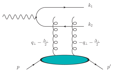
Figure 1: Diffractive dijet production in electron-ion collisions. Here we assume that the incoming virtual photon has only the longitudinal momentum. The signature of the diffractive process is the rapidity gap between the produced dijet and the target hadron which remains intact.

Now let us discuss diffractive dijet production in electron-ion collisions, which has been studied quite recently in Ref. Altinoluk:2015dpi , and demonstrate that it directly probes the dipole gluon GTMD. Diffractive events imply that a color neutral exchange must occur in the $t$-channel between the virtual photon and the target hadron over several units in rapidity. Following the same framework developed in Ref Dominguez:2011wm , by requiring that the final state quark-antiquark pair forms a color singlet state, we can write the cross section for diffractive dijet production as illustrated in Fig. 1 as follows

$$\frac{d\sigma^{\gamma_{T}^{\ast}A\rightarrow q\bar{q}X}}{dy_{1}d^{2}k_{1\perp}dy_{2}d^{2}k_{2\perp}} = 2N_{c}\alpha_{em}e_{q}^{2}\delta(x_{\gamma^{*}}-1)z(1-z)[z^{2}+(1-z)^{2}]\int d^{2}q_{\perp}d^{2}q_{\perp}^{\prime}\mathcal{F}_{x}(q_{\perp},\Delta_{\perp})\mathcal{F}_{x}(q_{\perp}^{\prime},\Delta_{\perp})$$ (11)

$$\times\left[\frac{P_{\perp}}{P_{\perp}^{2}+\epsilon_{f}^{2}}-\frac{P_{\perp}-q_{\perp}}{(P_{\perp}-q_{\perp})^{2}+\epsilon_{f}^{2}}\right]\cdot\left[\frac{P_{\perp}}{P_{\perp}^{2}+\epsilon_{f}^{2}}-\frac{P_{\perp}-q_{\perp}^{\prime}}{(P_{\perp}-q_{\perp}^{\prime})^{2}+\epsilon_{f}^{2}}\right]\ ,$$

for the transversely polarized photon. A similar cross section formula can be written for the longitudinally polarized photon. In Eq. (11), $y_{1,2}$ and $k_{1,2\perp}$ are rapidities and transverse momenta of the final state quark and antiquark jets, respectively, defined in the center of mass frame of the incoming photon and nucleon. $\vec{P}_{\perp}\equiv\frac{1}{2}(\vec{k}_{2\perp}-\vec{k}_{1\perp})$ represents the typical dijet transverse momentum and $\Delta_{\perp}$ is the nucleon recoiled momentum which equals to $-(k_{1\perp}+k_{2\perp})$ at leading order. We are interested in the back-to-back kinematic region for the two final state jets where $|P_{\perp}|\gg|\Delta_{\perp}|$. Suppose $\epsilon_{f}^{2}\equiv z(1-z)Q^{2}$ is not too large. Then we expect that the above $q_{\perp}$ integrals are dominated by the region $q_{\perp}\sim P_{\perp}$ and the cross sections are roughly proportional to $\mathcal{F}_{x}^{2}(P_{\perp},\Delta_{\perp})$ for back-to-back dijet configurations. Thus, the diffractive dijet production will be sensitive to the correlation between $P_{\perp}$ and $\Delta_{\perp}$ as mentioned in Ref. Altinoluk:2015dpi .

With the detector capability at the future EIC Accardi:2012qut , we will be able to identify both $\vec{P}_{\perp}$ and $\vec{\Delta}_{\perp}$ and measure the angular correlation between them. In particular, the elliptic angular correlation $\langle\cos 2\left(\phi_{P_{\perp}}-\phi_{\Delta_{\perp}}\right)\rangle$ can be observed in this process. By plugging in the $\cos 2\phi$ asymmetry in the gluon Wigner distributions from the numerical studies of Balitsky-Kovchegov evolution with impact parameter dependence GolecBiernat:2003ym ; Berger:2011ew , we find that it will lead to a few percent $\langle\cos 2\left(\phi_{P_{\perp}}-\phi_{\Delta_{\perp}}\right)\rangle$ asymmetries in the typical EIC kinematics. More sophistic calculations shall follow to generalize the saturation models Kowalski:2003hm ; Iancu:2003ge ; Watt:2007nr ; Rezaeian:2012ji to incorporate this particular angular correlation feature. We leave that for a future study. Comparing the theoretical computations with the future experimental data will provide us much more insights on the experimental signature of small-$x$ dynamics.

Summary and Discussions. To conclude, let us make some further but brief comments on the consequence of this work, while we will leave the detailed discussion for a future publication.

• In principle, as far as the gluon Wigner distribution is concerned, there should be correlation between the two vectors $\vec{q}_{\perp}$ and $\vec{b}_{\perp}$, which can be shown in theoretical studies for the dipole scattering amplitude in the small-$x$ region. In order to demonstrate this non-trivial correlation, we parametrize the above Wigner distribution as

  $$xW_{g}^{T}(x,\vec{q}_{\perp};\vec{b}_{\perp})=x{\cal W}_{g}^{T}(x,|\vec{q}_{\perp}|,|\vec{b}_{\perp}|)+2\cos(2\phi)x{\cal W}_{g}^{\epsilon}(x,|\vec{q}_{\perp}|,|\vec{b}_{\perp}|)+\cdots\ ,$$ (12)

  where $\phi$ is the azimuthal angle between $\vec{q}_{\perp}$ and $\vec{b}_{\perp}$. The first term above represents the azimuthal symmetric distribution, whereas the rest of other terms stand for the azimuthal asymmetric distribution. For example, due to the $\cos(2\phi)$ nature of the second term, we call it the Elliptic Gluon Wigner Distribution, and in short, elliptic gluon distribution. This is quite similar to the elliptic flow phenomena observed in heavy ion collisions.

• Let us further comment on the WW gluon distribution case. Following the same technique used above for the dipole gluon Wigner distribution, we generalize the WW gluon distribution at small-$x$ as follows

  $$xG_{\textrm{WW}}(x,q_{\perp},\Delta_{\perp})=2\int\frac{\text{d}\xi^{-}\text{d}^{2}\xi_{\perp}e^{-iq_{\perp}\cdot\xi_{\perp}-ixP^{+}\xi^{-}}}{\left(2\pi\right)^{3}P^{+}}\left\langle P+\frac{\Delta_{\perp}}{2}\left|\text{Tr}\left[F\left(\frac{\xi}{2}\right)\mathcal{U}^{\left[+\right]\dagger}F\left(-\frac{\xi}{2}\right)\mathcal{U}^{\left[+\right]}\right]\right|P-\frac{\Delta_{\perp}}{2}\right\rangle,$$ (13)

  which allows us to find

  $$xG_{\textrm{WW}}(x,q_{\perp},\Delta_{\perp}) = \frac{2N_{c}}{\alpha_{S}}\int\frac{d^{2}R_{\perp}}{(2\pi)^{2}}\frac{d^{2}R_{\perp}^{\prime}}{(2\pi)^{2}}\;e^{iq_{\perp}\cdot(R_{\perp}-R_{\perp}^{\prime})+i\frac{\Delta_{\perp}}{2}\cdot(R_{\perp}+R_{\perp}^{\prime})}$$ (14)

  $$\times\frac{1}{N_{c}}\left\langle\text{Tr}\left[i\partial_{i}U(R_{\perp})\right]U^{\dagger}(R_{\perp}^{\prime})\left[i\partial_{i}U(R_{\perp}^{\prime})\right]U^{\dagger}(R_{\perp})\right\rangle_{x}.$$

  Due to the known connection between the WW gluon distribution and color quadrupoles at small-$x$ Dominguez:2011wm , it is expected that one needs to generate a color quadrupole at the amplitude level in order to probe the WW Wigner distribution. This requires two incoming photons at once which produce four-jet diffractive events in the final states. It seems to be very challenging to measure this type of events at EIC. Nevertheless, it is more probable to perform such measurement in ultra-peripheral diffractive $AA$ collisions at the LHC where photons are much more abundant in the wavefunction of colliding nuclei.

• It is also interesting to note that one can generalize the above derivation to obtain the linearly polarized part Mulders:2000sh ; Boer:2010zf ; Qiu:2011ai ; Metz:2011wb ; Dominguez:2011br ; Sun:2011iw ; Boer:2011kf ; Dumitru:2015gaa of the WW and dipole gluon Wigner distribution when the indices of derivatives are off-diagonal, instead of diagonal as in Eqs. (1,2). The cross sections for dijet and four-jet productions depend on both the unpolarized and linearly polarized gluon distributions, which are related in the small-$x$ formalism Metz:2011wb ; Dominguez:2011br .

  In addition, when integrating over $q_{\perp}$ in Eqs. (1,2) with off-diagonal indices, the gluon Wigner distributions will reduce to the so-called helicity flip gluon GPDs (also called gluon transveristy), which have been extensively discussed in the collinear GPD framework Hoodbhoy:1998vm ; Belitsky:2000jk ; Diehl:2001pm ; Belitsky:2001ns . The nontrivial correlations between $q_{\perp}$ and $\Delta_{\perp}$ play important roles in the integral to obtain the helicity flip gluon GPDs.

The parton Wigner distributions, which contain the most complete information, are the cornerstones of all parton distributions. We demonstrate that gluon Wigner distributions are closely related to the impact parameter dependent dipole and quadrupole scattering amplitudes, and point out that they can be measured in diffractive type events at EIC and the LHC.

Acknowledgments: This material is based upon work supported by the U.S. Department of Energy, Office of Science, Office of Nuclear Physics, under contract number DE-AC02-05CH11231, and by the U.S. National Science Foundation under Grant No. PHY-0855561 and PHY-1417326. B.X. acknowledges interesting discussion with A. Mueller, and wishes to thank Dr. X.N. Wang and the nuclear theory group at LBNL for hospitality and support during his visit when this work is finalized.

References

- (1) D. Boer et al., arXiv:1108.1713 [nucl-th].
- (2) J. L. Abelleira Fernandez et al. [LHeC Study Group Collaboration], J. Phys. G 39, 075001 (2012).
- (3) A. Accardi et al., arXiv:1212.1701 [nucl-ex].
- (4) X. d. Ji, Phys. Rev. Lett. 91, 062001 (2003) [hep-ph/0304037].
- (5) A. V. Belitsky, X. d. Ji and F. Yuan, Phys. Rev. D 69, 074014 (2004) [hep-ph/0307383].
- (6) N. N. Nikolaev and B. G. Zakharov, Phys. Lett. B 332, 177 (1994) doi:10.1016/0370-2693(94)90876-1 [hep-ph/9403281].
- (7) J. Bartels, H. Lotter and M. Wusthoff, Phys. Lett. B 379, 239 (1996) [Phys. Lett. B 382, 449 (1996)] doi:10.1016/0370-2693(96)00412-1 [hep-ph/9602363].
- (8) J. Bartels, C. Ewerz, H. Lotter and M. Wusthoff, Phys. Lett. B 386, 389 (1996) doi:10.1016/0370-2693(96)81071-9 [hep-ph/9605356].
- (9) M. Diehl, Z. Phys. C 76, 499 (1997) doi:10.1007/s002880050573 [hep-ph/9610430].
- (10) V. M. Braun and D. Y. Ivanov, Phys. Rev. D 72, 034016 (2005) doi:10.1103/PhysRevD.72.034016 [hep-ph/0505263].
- (11) A. H. Rezaeian, M. Siddikov, M. Van de Klundert and R. Venugopalan, Phys. Rev. D 87, no. 3, 034002 (2013).
- (12) A. H. Mueller, Nucl. Phys. B 558, 285 (1999) [hep-ph/9904404].
- (13) F. Gelis, E. Iancu, J. Jalilian-Marian and R. Venugopalan, Ann. Rev. Nucl. Part. Sci. 60, 463 (2010); reference therein.
- (14) Y. V. Kovchegov and E. Levin, “Quantum chromodynamics at high energy,” (2012), Cambridge University Press.
- (15) I. I. Balitsky and L. N. Lipatov, Sov. J. Nucl. Phys. 28, 822 (1978) [Yad. Fiz. 28, 1597 (1978)]; L. N. Lipatov, Sov. J. Nucl. Phys. 23, 338 (1976) [Yad. Fiz. 23, 642 (1976)]; E. A. Kuraev, L. N. Lipatov and V. S. Fadin, Sov. Phys. JETP 44, 443 (1976) [Zh. Eksp. Teor. Fiz. 71, 840 (1976)] [Erratum-ibid. 45, 199 (1977)]; V. S. Fadin, E. A. Kuraev and L. N. Lipatov, Phys. Lett. B 60, 50 (1975).
- (16) S. Meissner, A. Metz and M. Schlegel, JHEP 0908, 056 (2009) [arXiv:0906.5323 [hep-ph]].
- (17) C. Lorce and B. Pasquini, JHEP 1309, 138 (2013) doi:10.1007/JHEP09(2013)138 [arXiv:1307.4497 [hep-ph]].
- (18) F. Dominguez, B. W. Xiao and F. Yuan, Phys. Rev. Lett. 106, 022301 (2011) [arXiv:1009.2141 [hep-ph]].
- (19) F. Dominguez, C. Marquet, B. W. Xiao and F. Yuan, Phys. Rev. D 83, 105005 (2011) [arXiv:1101.0715 [hep-ph]].
- (20) C. J. Bomhof, P. J. Mulders and F. Pijlman, Eur. Phys. J. C 47, 147 (2006).
- (21) A. V. Belitsky, X. Ji and F. Yuan, Nucl. Phys. B 656, 165 (2003).
- (22) L. N. Lipatov, Sov. Phys. JETP 63, 904 (1986) [Zh. Eksp. Teor. Fiz. 90, 1536 (1986)].
- (23) H. Navelet and R. B. Peschanski, Nucl. Phys. B 507, 353 (1997) doi:10.1016/S0550-3213(97)00568-3 [hep-ph/9703238].
- (24) H. Navelet and S. Wallon, Nucl. Phys. B 522, 237 (1998) doi:10.1016/S0550-3213(98)00146-1 [hep-ph/9705296].
- (25) I. Balitsky, Nucl. Phys. B 463, 99 (1996) [hep-ph/9509348].
- (26) Y. V. Kovchegov, Phys. Rev. D 60, 034008 (1999).
- (27) K. J. Golec-Biernat and A. M. Stasto, Nucl. Phys. B 668, 345 (2003) doi:10.1016/j.nuclphysb.2003.07.011 [hep-ph/0306279].
- (28) J. Berger and A. M. Stasto, Phys. Rev. D 84, 094022 (2011) doi:10.1103/PhysRevD.84.094022 [arXiv:1106.5740 [hep-ph]].
- (29) B. Z. Kopeliovich, H. J. Pirner, A. H. Rezaeian and I. Schmidt, Phys. Rev. D 77, 034011 (2008).
- (30) T. Altinoluk, N. Armesto, G. Beuf and A. H. Rezaeian, arXiv:1511.07452 [hep-ph].
- (31) H. Kowalski and D. Teaney, Phys. Rev. D 68, 114005 (2003) [hep-ph/0304189].
- (32) E. Iancu, K. Itakura and S. Munier, Phys. Lett. B 590, 199 (2004) [hep-ph/0310338].
- (33) G. Watt and H. Kowalski, Phys. Rev. D 78, 014016 (2008) doi:10.1103/PhysRevD.78.014016 [arXiv:0712.2670 [hep-ph]].
- (34) P. J. Mulders and J. Rodrigues, Phys. Rev. D 63, 094021 (2001) [arXiv:hep-ph/0009343].
- (35) D. Boer, S. J. Brodsky, P. J. Mulders, C. Pisano, Phys. Rev. Lett. 106, 132001 (2011). [arXiv:1011.4225 [hep-ph]].
- (36) J. -W. Qiu, M. Schlegel, W. Vogelsang, Phys. Rev. Lett. 107, 062001 (2011). [arXiv:1103.3861 [hep-ph]].
- (37) A. Metz and J. Zhou, Phys. Rev. D 84, 051503 (2011) doi:10.1103/PhysRevD.84.051503 [arXiv:1105.1991 [hep-ph]].
- (38) F. Dominguez, J. W. Qiu, B. W. Xiao and F. Yuan, Phys. Rev. D 85, 045003 (2012) [arXiv:1109.6293 [hep-ph]].
- (39) P. Sun, B. W. Xiao and F. Yuan, Phys. Rev. D 84, 094005 (2011) [arXiv:1109.1354 [hep-ph]].
- (40) D. Boer, W. J. den Dunnen, C. Pisano, M. Schlegel and W. Vogelsang, Phys. Rev. Lett. 108, 032002 (2012).
- (41) A. Dumitru, T. Lappi and V. Skokov, Phys. Rev. Lett. 115, no. 25, 252301 (2015) [arXiv:1508.04438 [hep-ph]].
- (42) P. Hoodbhoy and X. D. Ji, Phys. Rev. D 58, 054006 (1998) doi:10.1103/PhysRevD.58.054006 [hep-ph/9801369].
- (43) A. V. Belitsky and D. Mueller, Phys. Lett. B 486, 369 (2000) doi:10.1016/S0370-2693(00)00773-5 [hep-ph/0005028].
- (44) M. Diehl, Eur. Phys. J. C 19, 485 (2001) doi:10.1007/s100520100635 [hep-ph/0101335].
- (45) A. V. Belitsky, D. Mueller and A. Kirchner, Nucl. Phys. B 629, 323 (2002) doi:10.1016/S0550-3213(02)00144-X [hep-ph/0112108].