Binary-Fluid Turbulence: Signatures of Multifractal Droplet Dynamics and Dissipation Reduction

Abstract

We study the challenging problem of the advection of an active, deformable, finite-size droplet by a turbulent flow via a simulation of the coupled Cahn-Hilliard-Navier-Stokes (CHNS) equations. In these equations, the droplet has a natural two-way coupling to the background fluid. We show that the probability distribution function of the droplet center of mass acceleration components exhibit wide, non-Gaussian tails, which are consistent with the predictions based on pressure spectra. We also show that the droplet deformation displays multifractal dynamics. Our study reveals that the presence of the droplet enhances the energy spectrum $E(k)$, when the wavenumber $k$ is large; this enhancement leads to dissipation reduction.

I I. INTRODUCTION

The advection of droplets, bubbles, or particles by a fluid plays a central role in many natural and industrial settings jeremie2006 , which include clouds grabowski2013 ; shaw2003 , fuel injection fuel , microfluidics baroud2010 , inkjet printing inkjet , and the reduction of drag by bubbles lohse2003 . These studies require an accurate modeling of the motion of particles or droplets inside a turbulent fluid. The advection of finite-sized particles or droplets is especially challenging because they cannot be modelled as Lagrangian tracers bifarale2005 , or even like heavy-particles, which do not affect the motion of the carrier phase jeremie2006 .

Finite-size, deformable droplets affect the background fluid considerably, even as they are transported and deformed by the flow. This makes a systematic characterization of the statistical properties of turbulence difficult, because boundary conditions have to be implemented on the surface of the droplet, which changes as a function of time. The Cahn-Hilliard-Navier-Stokes (CHNS) equations that we use allow us to treat droplets elegantly via gradients in an order-parameter field $\phi$; therefore, we do not have to enforce complicated boundary conditions at the moving boundary between the droplet and the background fluid; and, we can follow the deformation of the droplet boundary in far greater detail than has been possible so far. Our ability to track this boundary, along with our efficient computer code on a GPU cluster has enabled us to show, among other things, that fluctuations of the droplet boundary are multifractal; this has not been investigated hitherto.

The simplest droplet-advection problem arises in a binary-fluid mixture, in which a droplet of the minority phase moves in the majority-phase background that is turbulent. We study this problem in two spatial dimensions (2D) by using the coupled CHNS equations, which have been used extensively in studies of critical phenomena, phase transitions chaikan2000 ; halperin77 ; lifshitz59 ; domb83 ; bray94 , nucleation nucleation , spinodal decomposition onuki2002 ; badalassi2003 ; perlekar2014 ; cahn61 ; bofetta2005 , and the late stages of phase separation bofetta2009 . We use the CHNS approach to carry out a detailed study of droplet dynamics in a turbulent flow and characterize the turbulence-induced deformation of a droplet and its acceleration statistics. We then elucidate the modification of fluid turbulence by the fluctuations of this droplet. Our study uses an extensive direct numerical simulation (DNS) of the CHNS equations in 2D, where we use parameters such that we have one droplet in our simulation domain. We track such a finite-sized droplet (for similar studies of Lagrangian or inertial particles see Ref. prasad2011 ) and obtain the statistics of the deformation of the droplet and its velocity and acceleration statistics as a function of the surface tension and size.

2D fluid turbulence, which is of central importance in many flows, is fundamentally different from its three-dimensional (3D) counterpart fjortoff ; Kraich ; Leith ; Batchelor ; leisure . The fluid-energy spectrum $E(k)$ in 2D turbulence shows (a) a forward cascade of enstrophy (or the mean-square vorticity), from the forcing wave number $k_{f}$ to wave numbers $k>k_{f}$ and (b) an inverse cascade of energy to $k<k_{f}$. We use parameters that lead to an $E(k)$ that is dominated by a forward-cascade regime. Our study leads to new insights and remarkable results: we show that the turbulence-induced fluctuations in the dimensionless deformation of the droplet are intermittent. We characterize this intermittency of the droplet fluctuations by obtaining the probability distribution function (PDF) $P_{\Gamma}(\Gamma)$ and the multifractal spectrum $f_{\Gamma}(\alpha)$ of the time series $\Gamma(t)$. We show that the PDF of the components of the acceleration of the center of mass are similar to those for finite-size particles in turbulent flows jeremie and are consistent with predictions based on pressure spectra hill ; qureshi2007 . We also find that the large-$k$ tail of $E(k)$ is enhanced by the droplet fluctuations; this leads to dissipation reduction, in much the same way as in turbulent fluids with polymer additives kalelkar05 ; perlekar06 ; gupta15 . The spectrum $E(k)$ also displays oscillations whose period is related inversely to the mean diameter of the droplet. We show that such oscillations appear prominently in the order-parameter spectrum $S(k)$, which is the Fourier transform of the spatial correlation function of $\phi$, the Cahn-Hilliard scalar field that distinguishes between the two binary-fluid phases.

The remainder of the paper is organized as follows. Section II introduces the CHNS equations and the numerical methods we use to solve them. We present the results of our DNS in Section III, which comprises subsections on (a) droplet-deformation statistics, (b) droplet-acceleration statistics, (c) energy-dissipation time series and energy and order-parameter spectra. Section IV contains a discussion of our results and conclusions. An Appendix contains some details of our calculations.

II II. MODEL AND NUMERICAL METHODS

Two-way coupling, between the droplet and the background turbulent fluid, appears naturally in the CHNS equations celani2009 ; scarbolo2013 ; shen2004 ; scarbolo2011 . In 2D, the Navier-Stokes equations can be written in the following stream-function vorticity formulation  bofetta2009 :

$$\left(\partial_{t}+{\bm{u}}\cdot\nabla\right)\omega = \nu\nabla^{2}\omega-\alpha\omega-\nabla\times(\phi\nabla\mu)+F_{\omega};$$ (1)

$$\left(\partial_{t}+{\bm{u}}\cdot\nabla\right){\bf\phi} = \gamma\nabla^{2}{\mu}~{}{\rm{and}}~{}\nabla\cdot{\bm{u}}=0.$$ (2)

Here ${\bm{u}}\equiv(u_{x},u_{y})$ is the fluid velocity, $\omega$ is the vorticity, $\mu$ is the chemical potential; $\omega$ and $\mu$ are connected to ${\bm{u}}$ and $\phi$ in the following way:

$$\omega = (\nabla\times{\bm{u}}){\hat{\bm{e}}}_{z},$$ (3)

$$\mu({\bm{x}},t) = \delta{\mathcal{F}}[\phi]/\delta\phi,$$ (4)

$${\mathcal{F}}[\phi] = \Lambda\int[(\phi^{2}-1)^{2}/(4\xi^{2})$$ (5)

$$+|\nabla\phi|^{2}/2]d{\bm{x}}\phi({\bm{x}},t),$$

where ${\mathcal{F}}[\phi]$ is the free energy. In Eqs. (1)-(2) $\Lambda$ is the energy density with which the two phases mix in the interfacial regime celani2009 , $\xi$ sets the scale of the diffuse interface width, $\nu$ is the kinematic viscosity, $\gamma$ is the mobility shen2004 of the binary-fluid mixture, $F_{\omega}=F_{0}\cos(k_{f}y)$ is a Kolmogorov-type forcing kolmogorov with amplitude $F_{0}$ and forcing wave number $k_{f}$, and $\alpha$ is the air-drag induced friction. For simplicity, we concentrate on mixtures in which $\gamma$ is independent of $\phi$ and both components have the same density and viscosity. In our model, $\sigma=\frac{2\sqrt{2}\Lambda}{3\xi}$ is the surface tension. The Grashof number $Gr=\frac{L^{4}F_{0}}{\nu^{2}}$ is a convenient dimensionless ratio of the forcing and viscous terms. We keep the diffusivity $D=\frac{\gamma\beta}{\xi^{2}}$ of the system constant. The forcing-scale Weber number $We\equiv\rho L_{f}^{3}F_{0}/\sigma$, where $L_{f}=2\pi/k_{f}$, is a natural dimensionless measure of the inverse of the surface tension.

The minority and majority phases in our model is described by an order-parameter field $\phi({\bm{x}},t)$ at the point ${\bm{x}}$ and time $t$ with $\phi({\bm{x}},t)>0$ in the background (majority) phase and $\phi({\bm{x}},t)<0$ in the droplet (minority) phase (see Fig. 1(a)). At time $t=0$ we begin with the order-parameter profile celani2009 ; scarbolo2011

$$\phi(x,y)=\tanh\left[\frac{1}{\sqrt{2}\xi}\left(\sqrt{(x-x_{c})^{2}+(y-y_{c})^{2}}-d_{0}/2\right)\right],$$ (6)

which ensures that the droplet is circular at $t=0$, with its center at $(x_{c},y_{c})$, diameter $d_{0}$, and has a diffuse interface, because $\phi$ change continuously in the interface. The interface width $\xi$ is measured by the dimensionless Cahn number $Ch=\xi/L$.

Our direct numerical simulations (DNSs) of Eqs. (1) and (2) use a pseudospectral method and periodic boundary conditions; $L(=2\pi)$ is the linear size of our square simulation domain which has $N^{2}$ collocation points. We have a cubic nonlinearity in the chemical potential $\mu$ (Eq. 2), so we use $N/2$-dealiasing spectral . For time integration we use the exponential Adams-Bashforth method ETD2 cox2002 . We use computers with Graphics Processing Units (e.g., the NVIDIA K80), which we program in CUDA cuda ; our efficient code allows us to explore the CHNS parameter space and carry out very long simulations that are essential for our studies. In the following paragraph we introduce the quantities that we calculate from the fields $\omega({\bm{x}},t)$ and $\phi({\bm{x}},t)$, which we obtain from our DNSs of Eqs. (1) and (2).

From the field $\phi({\bm{x}},t)$ we calculate the droplet deformation parameter which we define as perlekar12 ,

$$\Gamma(t)=\frac{{\mathcal{S}}(t)}{{\mathcal{S}}_{0}(t)}-1,$$ (7)

where ${\mathcal{S}}(t)$ is the perimeter of the droplet (the $\phi=0$ contour) at time $t$, ${\mathcal{S}}_{0}(t)$ is the perimeter of an undeformed droplet of equal area at $t$. From the field $\omega({\bm{x}},t)$ we calculate the total kinetic energy of the fluid $E(t)$, and the fluid-energy dissipation rate $\varepsilon(t)$, which are

$$E(t) = \langle|{\bm{u}}({\bm{x}},t)|^{2}\rangle_{{\bm{x}}},$$ (8)

$$\varepsilon(t) = \langle\nu|\omega({\bm{x}},t)|^{2}\rangle_{{\bm{x}}},$$ (9)

where $\langle\rangle_{{\bm{x}}}$ denotes the average over space. From $E(t)$ and $\varepsilon(t)$ we calculate the root-mean-square fluid velocity, $u_{rms}=\sqrt{\langle 2E(t)\rangle_{t}}$, where $\langle\rangle_{t}$ denotes the average over the statistically steady, but turbulent state with small fluctuations about the mean value, i.e, the fluid is in the statistically stationary state. From these, we calculate the Taylor-microscale Reynolds number $Re_{\lambda}(t)=\sqrt{2}E(t)/\sqrt{\nu\varepsilon(t)}$, and the mean $\langle Re_{\lambda}\rangle_{t}$, which characterizes the intensity of turbulence and the box-size eddy-turnover time $\tau_{eddy}=L/u_{rms}$; we express time in units of $\tau_{eddy}$. We calculate the energy spectra $E(k)$ and order-parameter (or phase-field) spectra $S(k)$ as follows:

$$E(k) \equiv \sum\limits_{k-\frac{1}{2}\leq k^{\prime}\leq k+\frac{1}{2}}\langle|\hat{\bm{u}}({\mathbf{k}}^{\prime},t)|^{2}\rangle_{t},$$ (10)

$$S(k) \equiv \sum\limits_{k-\frac{1}{2}\leq k^{\prime}\leq k+\frac{1}{2}}\langle|\hat{\phi}({\mathbf{k}}^{\prime},t)|^{2}\rangle_{t},$$ (11)

where $\hat{\bm{u}}({\mathbf{k}}^{\prime},t)$ and $\hat{\phi}({\mathbf{k}}^{\prime},t)$ are, respectively, the spatial Fourier transforms of ${\bm{u}}({\bm{x}},t)$ and $\phi({\bm{x}},t)$. We have carried out several DNSs (R1-R28) that are given in Table I.

	$Gr$	$d_{0}/L$	$We$	$\langle d_{p}\rangle_{t}/L$	$\langle\lambda\rangle_{t}/L$	$\langle\eta\rangle_{t}/L$	$\langle E\rangle_{t}$	$\langle\varepsilon\rangle_{t}$	$\langle Re_{\lambda}\rangle_{t}$
R1	$3\times 10^{7}$						$1.9$	$0.017$	$216$
R2	$3\times 10^{7}$	$0.332$	$1.38$	$0.324$	$0.08$	$0.007$	$1.17$	$5.4$	$112$
R3	$3\times 10^{7}$	$0.312$	$1.38$	$0.3$	$0.08$	$0.007$	$1.24$	$5.1$	$120$
R4	$3\times 10^{7}$	$0.293$	$1.38$	$0.283$	$0.09$	$0.007$	$1.3$	$4.9$	$127$
R5	$3\times 10^{7}$	$0.273$	$1.38$	$0.263$	$0.09$	$0.007$	$1.36$	$0.023$	$137.5$
R6	$3\times 10^{7}$	$0.25$	$1.38$	$0.245$	$0.09$	$0.007$	$1.4$	$4.4$	$146.5$
R7	$3\times 10^{7}$	$0.24$	$5.34$	$0.2$	$0.1$	$0.007$	$1.4$	$4.63$	$140$
R8	$3\times 10^{7}$	$0.24$	$2.3$	$0.22$	$0.11$	$0.007$	$1.44$	$4.35$	$151$
R9	$3\times 10^{7}$	$0.24$	$1.97$	$0.22$	$0.11$	$0.007$	$1.45$	$4.2$	$153.4$
R10	$3\times 10^{7}$	$0.24$	$1.84$	$0.22$	$0.11$	$0.007$	$1.48$	$4.25$	$154.7$
R11	$3\times 10^{7}$	$0.24$	$1.53$	$0.22$	$0.11$	$0.007$	$1.48$	$4.45$	$157.4$
R12	$3\times 10^{7}$	$0.24$	$1.38$	$0.22$	$0.12$	$0.007$	$1.47$	$4.21$	$157$
R13	$3\times 10^{7}$	$0.24$	$0.534$	$0.22$	$0.12$	$0.007$	$1.5$	$4.19$	$160$
R14	$3\times 10^{7}$	$0.24$	$0.138$	$0.22$	$0.12$	$0.007$	$1.5$	$4.22$	$162$
R15	$3\times 10^{7}$	$0.215$	$1.38$	$0.21$	$0.13$	$0.007$	$1.57$	$4.15$	$168$
R16	$3\times 10^{7}$	$0.2$	$1.38$	$0.177$	$0.13$	$0.007$	$1.62$	$3.96$	$177$
R17	$3\times 10^{7}$	$0.174$	$1.38$	$0.153$	$0.14$	$0.007$	$1.7$	$3.8$	$188$
R18	$3\times 10^{7}$	$0.14$	$5.34$	$0.097$	$0.15$	$0.007$	$1.8$	$3.83$	$200$
R19	$3\times 10^{7}$	$0.14$	$2.3$	$0.125$	$0.15$	$0.007$	$1.75$	$3.83$	$195$
R20	$3\times 10^{7}$	$0.14$	$1.38$	$0.126$	$0.15$	$0.007$	$1.75$	$3.7$	$193$
R21	$3\times 10^{7}$	$0.134$	$0.52$	$0.09$	$0.153$	$0.007$	$1.84$	$3.78$	$205$
R22	$1.5\times 10^{8}$				$0.12$	$0.005$	$12.5$	$23.8$	$561.7$
R23	$1.5\times 10^{8}$	$0.24$	$0.138$	$0.22$	$0.094$	$0.005$	$9.08$	$27.1$	$381.4$
R24	$1.5\times 10^{8}$	$0.215$	$0.138$	$0.2$	$0.1$	$0.005$	$9.5$	$25.4$	$411$
R25	$1.5\times 10^{8}$	$0.2$	$0.138$	$0.176$	$0.104$	$0.005$	$10.2$	$25.1$	$444$
R26	$1.5\times 10^{8}$	$0.174$	$0.138$	$0.1525$	$0.108$	$0.005$	$10.7$	$23.9$	$477.8$
R27	$1.5\times 10^{8}$	$0.14$	$0.138$	$0.125$	$0.112$	$0.005$	$11.67$	$24.3$	$516.8$
R28	$1.5\times 10^{8}$	$0.134$	$0.138$	$0.083$	$0.116$	$0.005$	$12.2$	$23.8$	$545.1$

Table 1: The parameters $Gr$, $d_{0}$, $We$, $\langle d_{p}\rangle_{t}/L$, $\langle\lambda\rangle_{t}/L$, $\langle\eta\rangle_{t}/L$, $\langle E\rangle_{t}$, $\langle\varepsilon\rangle_{t}$, and $\langle Re_{\lambda}\rangle_{t}$ for our DNS runs R1-R28. The number of collocation points is kept fixed at $N^{2}=1024^{2}$ in each direction. The friction coefficient $\alpha=0.001$, the forcing wave number is fixed at $k_{f}=3$, $\nu=4.67\times 10^{-3}$ is the kinematic viscosity, the diffusivity $D=4\times 10^{-3}$, $d_{0}/L$ is the non-dimensional droplet diameter at the initial time, the forcing-scale Weber number $We\equiv\rho L_{f}^{3}F_{0}/\sigma$, where $\sigma$ is the surface tension, the Cahn number $Ch=\xi/L$, where $\xi$ is the interface width, is kept fixed at $Ch=0.0028$, $\langle d_{p}\rangle_{t}/L$ is the steady-state droplet diameter non-dimensionalized with the box length $L$, the dissipation scale $\eta=\left(\nu^{3}/\varepsilon\right)^{\frac{1}{4}}$, where $\varepsilon$ is the fluid-energy dissipation rate ($\varepsilon(t)=\langle\nu|\omega({\bm{x}},t)|^{2}\rangle_{{\bm{x}}}$), $E(t)=\langle|{\bm{u}}({\bm{x}},t)|^{2}\rangle_{{\bm{x}}}$ is the fluid kinetic energy, and $Re_{\lambda}$ the Taylor-microscale Reynolds number. In all cases $\langle\rangle_{t}$ denotes the average over time in the statistically steady state.

III III. RESULTS

Our investigations of droplet dynamics are divided into two broad categories. We first elucidate the turbulence-induced modification of the droplet in subsections A and B. Then we show how the droplet modifies various statistical properties of turbulence, such as $E(k)$, in subsection C.

III.1 A. Droplet deformation statistics

We use Eq. (7) for $\Gamma(t)$ and obtain $\mathcal{S}(t)$ by finding the length of the $\phi=0$ contour and the area $A(t)$ inside the $\phi=0$ contour. We then calculate $d_{p}(t)=2\sqrt{A(t)/\pi}$, an effective diameter for the droplet that is not circular in general. Given the initial profile (6), we find that $\langle d_{p}\rangle_{t}<d_{0}$, and $\langle d_{p}\rangle_{t}$ increases roughly linearly with $d_{0}$. In Fig. 1(b) we plot the perimeter ${\mathcal{S}}(t)$ (deep-blue line), area $A(t)$ (light-blue line), the perimeter ${\mathcal{S}}_{0}(t)$ of a circular droplet of area $A$ (green line), and the deformation parameter $\Gamma(t)$ (red line) for the run R7 with $We=5.34$. This plot shows that the instantaneous total area $A(t)$ of the minority phase decreases very little over the entire duration of our simulation. $A(t)$ is almost constant and just fluctuates about its mean value $\langle A(t)\rangle_{t}$; these fluctuations do not contribute significantly to the deformation statistics because they are much smaller than the fluctuations in the droplet perimeter ${\mathcal{S}}(t)$. (We expect that, in the limit of zero mobility and constant surface tension (i.e., the sharp-interface limit), the mass transfer is negligible, and $A(t)$ is independent of $t$.)

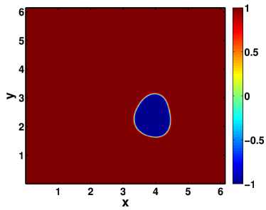
Figure 1: (Color online) (a)Pseudocolor plot of the $\phi$ field; (b) plots versus $t/\tau_{eddy}$ of the perimeter ${\mathcal{S}}(t)$ (deep-blue line), area $A(t)$ (light-blue line), perimeter ${\mathcal{S}}_{0}(t)$ (green line), of a circular droplet of area $A(t)$, and the deformation parameter $\Gamma(t)$ (red line) for the run R7 ($We=5.34$).

Our droplet diameters are comparable to lengths in the inertial range, which lies in between the large forcing length scale and the small scales where dissipation is significant. Turbulence induces large fluctuations in the shape of a droplet, so we integrate Eqs.(1) and (2) for $2000\tau_{eddy}$, to obtain the time series of the dimensionless deformation $\Gamma(t)$, which we depict in Figs. 2(a), for different values of $We$. Not only does the mean $\langle\Gamma\rangle_{t}$ increase as $We$ increases, so do the variance, skewness, and kurtosis of this time series. In particular, the root-mean-square value $\Gamma_{rms}=\langle\left(\Gamma-\langle\Gamma\rangle_{t}\right)^{2}\rangle_{t}$ increases with $We$ ($\Gamma_{rms}=0.14$ for $We=5.34$, $\Gamma_{rms}=0.033$ for $We=2.3$ and $\Gamma_{rms}=0.016$ for $We=1.38$), as do the skewness $\gamma_{1}=\langle\left(\Gamma-\langle\Gamma\rangle_{t}\right)^{3}\rangle_{t}/\langle\left(\Gamma-\langle\Gamma\rangle_{t}\right)^{2}\rangle_{t}^{3/2}$ ($\gamma_{1}=2.9$ for $We=5.34$, $\gamma_{1}=1.57$ for $We=2.3$ and $\gamma_{1}=0.8$ for $We=1.38$) and the kurtosis $\gamma_{2}=\langle\left(\Gamma-\langle\Gamma\rangle_{t}\right)^{4}\rangle_{t}/\langle\left(\Gamma-\langle\Gamma\rangle_{t}\right)^{2}\rangle_{t}^{2}$ ($\gamma_{2}=22.4$ for $We=5.34$, $\gamma_{2}=7.5$ for $We=2.3$ and $\gamma_{2}=5.8$ for $We=1.38$). We find that $\Gamma_{rms},\gamma_{1}$, and $\gamma_{2}$ decrease as $We$ decreases (i.e., the surface tension $\sigma$ increases) and the droplet becomes rigid.

From the time series of $\Gamma(t)$ we find the PDF $P_{\Gamma}(\Gamma)$ (Fig. 2(b)). These plots quantify the intuitively appealing result that the fluctuations of the droplet increase with an increase in $We$ (i.e., decrease with an increase in $\sigma$). The right tail of $P_{\Gamma}(\Gamma)$ decays exponentially with $\Gamma$; this decay steepens as $We$ decreases, and $P_{\Gamma}(\Gamma)$ sharpens, as it must, for there can be no shape fluctuations if $We=0$ (a perfectly rigid droplet).

The time series of $\Gamma(t)$ and the large kurtosis of $P_{\Gamma}(\Gamma)$ suggest intermittency; we characterize this intermittency by obtaining the multifractal spectrum (see Refs.muzy1993 ; ashken ; physionet ) $f_{\Gamma}(\alpha)$ (Fig. 2(c)), which is the Legendre transform of the Renyi exponents $\tau(q)$ that follow from $\langle|\Gamma(0)-\Gamma(t)|\rangle^{q}\sim t^{\tau(q)}$. This remarkable multifractality of $\Gamma(t)$ has not been noted so far. As $We$ decreases ($\sigma$ increases), the droplet-shape fluctuations decrease and the value of $\alpha$, at which $f_{\Gamma}(\alpha)$ attains a maximum, shifts towards $0$. If $\sigma$ is low, the droplet can break up at certain times, but the broken fragments coalesce to form a single drop again. The break-up events can be identified from the largest spikes in $\Gamma(t)$, because the formation of small droplets increases the total perimeter. Such droplet breakups occur only with the smallest value of $\sigma$ that we consider, and then only for about $4\%$ of the total time. We give an outline of the method we use to obtain multifractal spectra in the Appendix, where we follow Refs. muzy1993 ; ashken ; physionet .

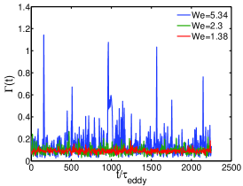
Figure 2: (Color online) (a) Plots versus $t/\tau_{eddy}$ of $\Gamma(t)$ for the runs R7 ($We=5.34$, blue line), R8 ($We=2.3$, green line) and R12 ($We=1.38$, red line); (b) plots of the PDFs $P(\Gamma)$, for the runs R7 ($We=5.34$, blue line with circles), R8 ($We=2.3$, green line with circles) and R13 ($We=1.38$, red line with circles); (c) the multifractal spectra $f_{\Gamma}(\alpha)$ for the timeseries of $\Gamma$ for the runs R7 ($We=5.34$, blue circles), R8 ($We=2.3$, green squares) and R13 ($We=1.38$, red diamonds). The insets in (a) show pseudocolor plots of the vorticity field with $\phi$-field contours superimposed on them; the time evolution of such plots are given in the videos V1 and V2 in Ref. suppmat

III.2 B. Droplet center-of-mass acceleration statistics

We now investigate the advection of the droplet inside the background fluid. To quantify droplet advection, we obtain PDFs of the components of the acceleration of the center of mass of the droplet along its trajectory biferale13conf . We obtain the center of mass velocity ${\bf v}_{CM}$ of the droplet and $a_{y}$, the $y$ component of the acceleration of the droplet center of mass, where

$${\bf v}_{CM}(t) = \sum\limits_{{\bm{x}}\ni\phi({\bm{x}},t)<0}{\bm{u}}({\bm{x}},t)$$ (12)

$${\rm and}\qquad a_{y}(t) = \sum\limits_{{\bm{x}}\ni\phi({\bm{x}},t)<0}(Du_{y}({\bm{x}},t)/Dt).$$ (13)

Note that $\phi({\bm{x}},t)<0$ if ${\bm{x}}$ lies inside the droplet at time $t$, and $D/Dt=\partial_{t}+{\bm{u}}\cdot\nabla$. We present results for $a_{y}$ (the results for the $x$ component $a_{x}$ are similar), and the root-mean-square acceleration $a_{rms}=\sqrt{a_{y}^{2}+a_{x}^{2}}$. We restrict ourselves to values of $\sigma$ for which there is a single droplet in the flow; and we use $10$ different values of $d_{0}$ in the range $0.134L$ to $0.334L$. In Fig. 3(a) we plot the PDF $P(a_{y})$ for four different values of $We$ at $d_{0}/L=0.24$. These PDFs collapse on top of each other (Fig. 3(a)), so, in a statistical sense, the center of mass of a deformable droplet moves in the same way as a rigid droplet. Indeed, $P(a_{y})$ is very close to a Gaussian (black dashed line), for droplets with $d_{0}/L=0.24$. From Eq. (13) we see that the acceleration of the center of mass of the droplet follows from an integral over the area of the droplet. For a rigid droplet, whose diameter is comparable to inertial-range scales, we expect the small-scale fluctuations to be averaged out and $P(a_{y})$ to be close to a Gaussian. We do, indeed, find this, for several values of $We$, in Fig. 3(a), where $\langle d_{p}\rangle_{t}/L=0.22$. By contrast, when we reduce $\langle d_{p}\rangle_{t}/L$, this PDF shows significant deviations from a Gaussian form as we show in Fig. 3(b).

Our results for $P(a_{y})$ are in qualitative accord with those for the advection of a rigid particle by a three-dimensional (3D), homogeneous and isotropic turbulent flow jeremie , for particle diameters in the inertial range: References jeremie ; qureshi2007 suggest that plots of the velocity variance $|\frac{|{\bf v}_{CM}|^{2}-u_{rms}^{2}}{u_{rms}^{2}}|$, $\langle a_{y}^{2}\rangle$, and $\langle a_{rms}\rangle_{t}$ versus the scaled particle diameter $\left(\langle d_{p}\rangle_{t}/L\right)$ should exhibit power laws with exponents that can be related to the inertial-range, power-law exponent in the pressure spectrum. We adapt these arguments to our study of a droplet, with mean scaled diameter $\langle d_{p}\rangle_{t}/L$. The plot in Fig. 3(c) is consistent with a power-law dependence of $\langle a_{rms}\rangle_{t}$ on $\langle d_{p}\rangle_{t}/L$, albeit over a small range jeremie_footnote , with exponents that can be related to the inertial-range scaling of the pressure spectrum. If the pressure spectrum of the turbulent fluid with a droplet is $|\tilde{\mathcal{P}}(k)|^{2}\sim k^{-\alpha_{\mathcal{P}}}$, for $k$ in the scaling range, then $\langle a_{rms}\rangle_{t}\sim\left(\langle d_{p}\rangle_{t}/L\right)^{\frac{\alpha_{\mathcal{P}}-3}{2}}$. We give details of the relation between the pressure-spectrum scaling and the plot of the acceleration variance versus the non-dimensionalized droplet diameter scaling below.

Our simulations suggest that $\langle a_{rms}\rangle\sim\left(\langle d_{p}\rangle_{t}/L\right)^{-1.06}$. Here we provide arguments that suggest such a power-law dependence; we follow the treatment of Refs. jeremie ; qureshi2007 for rigid particles. We first define the structure function for increments of the pressure $\mathcal{P}$ as

$$S_{2}^{{\mathcal{P}}}({\mathbf{r}})=\langle\left({\mathcal{P}}({\mathbf{x}})-{\mathcal{P}}({\mathbf{x}}+{\mathbf{r}})\right)^{2}\rangle\sim r^{\zeta_{2}^{{\mathcal{P}}}},$$ (14)

for separations $r$ in the inertial range. If we introduce $\tilde{{\mathcal{P}}}({\mathbf{k}})=(1/4\pi^{2})\int d{\mathbf{x}}e^{i{\mathbf{x.k}}}{\mathcal{P}}({\mathbf{x}})$, the spatial Fourier transform of ${\mathcal{P}}({\mathbf{r}})$, we have

$$S_{2}^{{\mathcal{P}}}({\mathbf{r}}) = \langle{\mathcal{P}}({\bf x}+{\bf r})\rangle^{2}+\langle{\mathcal{P}}({\bf x})\rangle^{2}-2\langle{\mathcal{P}}({\bf x}+{\bf r}){\mathcal{P}}({\bf x})\rangle,$$ (15)

$$= 2\int\limits_{0}^{\infty}dk|\tilde{\mathcal{P}}(k)|^{2}-\int\limits_{0}^{\infty}dk|\tilde{\mathcal{P}}(k)|^{2}\int\limits_{0}^{2\pi}e^{-ikrcos\theta}d\theta,$$

$$= 2\int\limits_{0}^{\infty}dk|\tilde{\mathcal{P}}(k)|^{2}\left(1-\pi I_{0}(r)\right),$$

where $I_{0}(r)=\sum\limits_{m=0}^{\infty}\frac{1}{m!\Gamma(m+1)}\left(\frac{r}{2}\right)^{2m}$ is the modified Bessel function of the first kind. If we have the inertial-range scaling form $|\tilde{\mathcal{P}}(k)|^{2}\sim k^{-\alpha^{p}}$, then the exponent

$$\alpha^{\mathcal{P}}=\zeta^{\mathcal{P}}_{2}+1.$$ (16)

In the velocity formulation of the NS equation

$$\left(\partial_{t}+{\bm{u}}\cdot\nabla\right){\bm{u}}=-\nabla{\mathcal{P}}/\rho+\nu\nabla^{2}{\bm{u}}-\alpha{\bm{u}}-(\phi\nabla\mu)+F_{\bm{u}},$$ (17)

we can assume that, in the inertial range, the main contribution to the right-hand side of Eq.( 1) comes from (we take $\rho=1$) $-\nabla{\mathcal{P}}-(\phi\nabla\mu)\equiv-\nabla{\mathcal{P}}^{\prime}$. We have introduced ${\mathcal{P}}^{\prime}$, so we now work with primed exponents $\alpha^{\mathcal{P}^{\prime}}$ and $\zeta_{2}^{\mathcal{P}^{\prime}}$, which can be defined like their counterparts without the primes. From Refs. qureshi2007 ; hill we know that

$$\langle a_{rms}^{2}\rangle \sim \langle\left(\left(\partial_{t}+{\bm{u}}\cdot\nabla\right){\bm{u}}\right)^{2}\rangle$$ (18)

$$\sim \langle\nabla{\mathcal{P}}^{\prime}({\bf{x}}+{\bf r})\nabla{\mathcal{P}}^{\prime}({\bf x})\rangle$$

$$\sim S_{2}^{\mathcal{P}^{\prime}}({\bf r})/r,$$

so we have the scaling results

$$\langle a_{rms}\rangle\sim\sqrt{S_{2}^{\mathcal{P}^{\prime}}({\mathbf{r}})}/r\sim r^{\zeta_{2}^{\mathcal{P}^{\prime}}/2}/r\sim r^{\frac{\alpha^{\mathcal{P}^{\prime}}-3}{2}}.$$ (19)

From our simulations we find $\alpha^{\mathcal{P}^{\prime}}\simeq 1.2$ (Fig. 3(d)), which implies $\langle a_{rms}\rangle\sim r^{-0.9}$, which is consistent, given our error bars, with our measured value of $-1.06$ (Fig. 3(b)); here $\langle d_{p}\rangle_{t}/L$ plays the role of $r$ in our scaling arguments.

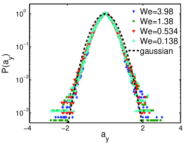
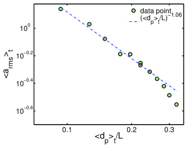
Figure 3: (Color online) (a) Semilog (base $10$) plots at $Gr=3\times 10^{7}$ of $P(a_{y})$, the PDF of $a_{y}$ of the center of mass of the droplets, for runs R8 ($We=2.3$, deep-blue diamonds), R12 ($We=1.38$, green squares), R13 ($We=0.534$, red inverted triangles) and R14 ($We=0.138$, light-blue triangles), at $\langle d_{p}\rangle_{t}/L=0.22$; (b) R20 ($\langle d_{p}\rangle_{t}/L=0.126$, deep-blue circles), R17 ($\langle d_{p}\rangle_{t}/L=0.153$, green diamonds), R12 ($\langle d_{p}\rangle_{t}/L=0.22$, red squares), R5 ($\langle d_{p}\rangle_{t}/L=0.263$, light-blue inverted triangles), R4 ($\langle d_{p}\rangle_{t}/L=0.283$, magenta plus signs) and R2 ($\langle d_{p}\rangle_{t}/L=0.324$, yellow asterisk) at $We=1.38$; (c) plot of $\langle a_{rms}\rangle_{t}$ versus $\langle d_{p}\rangle_{t}/L$; (d) Log-log plots (base $10$) versus the scaled wavenumber $k/k_{max}$ of the pressure spectrum $|\mathcal{P}(k)|^{2}$ for runs R12 ($\langle d_{p}\rangle_{t}/L=0.22$, deep-blue line with circles), R17 ($\langle d_{p}\rangle_{t}/L=0.177$, green line with circles), R1 (single-phase fluid, red line with circles), power-law scaling $k^{-1.2}$ (light-blue and magenta dash-dot line) and $k^{-9}$ (yellow dash-dot line). In (a) and (b) the black dashed line shows a Gaussian fit.

III.3 C. Energy-dissipation time series and energy and order-parameter spectra

The inertial-range size of our droplet ensures that the background fluid is perturbed by it. To explore how the droplet affects the turbulence, we first present log-log plots of the energy spectra $E(k)$ (with and without the droplet) versus the scaled wavenumber $k/k_{max}$, where $k_{max}=N/4$ is the maximum wavenumber in our dealiased DNS. We find that $E(k)$ is modified in two important ways by the droplet : (1) $E(k)$ shows oscillations whose period is related inversely to $\langle d_{p}\rangle_{t}$; (2) the large-$k$ tail of $E(k)$ is enhanced by the droplet spectrum_footnote . This enhancement is similar to that in fluid turbulence with polymer additives gupta15 ; and it can be understood by introducing the scale-dependent effective viscosity $\nu_{eff}(k)=\nu+\Delta\nu(k)$ (in Fourier space), with

$$\Delta\nu(k)\equiv\sum\limits_{k-1/2<k^{\prime}\leq k+1/2}\frac{{\mathbf{u}}_{{\mathbf{k}}^{\prime}}.\left(\phi\bigtriangledown\mu\right)_{-{\mathbf{k}}^{\prime}}}{k^{2}E(k)}$$ (20)

and $\left(\phi\bigtriangledown\mu\right)_{{\mathbf{k}}}$ the Fourier transform of $\left(\phi\bigtriangledown\mu\right)$ (Eqs. (1)-(2)). In the inset of Fig. 4(a) we plot $\Delta\nu(k)$ versus $k/k_{max}$ for the illustrative case $\langle d_{p}\rangle_{t}/L=0.324$ (deep-blue line with asterisks); when $\Delta\nu(k)>0$, $E(k)$ is less than its single-phase-fluid value (magenta curve); and when $\Delta\nu(k)<0$, $E(k)$ is greater than its single-phase-fluid value. The change in the sign of $\Delta\nu$ occurs at a value of $k/k_{max}$ that depends on $\langle d_{p}\rangle_{t}/L$; the smaller the value of $\langle d_{p}\rangle_{t}/L$, the larger is the value of $k/k_{max}$ at which $\Delta\nu(k)$ goes from being positive to negative. As $\langle d_{p}\rangle_{t}/L$ increases, $E(k)$ falls less steeply with $k$ in the power-law range; e.g., $E(k)\sim k^{-5.2}$ if there is no droplet and $E(k)\sim k^{-3.6}$ if $\langle d_{p}\rangle_{t}/L=0.324$. Because we use a friction term, in the inertial range $E(k)$ scales as $\simeq k^{-5.2}$, which is considerably different from $-3$, the exponent in the limit of no friction perlekar09 ; bofetta12 . At low $k$, $E(k)$ decreases as $\langle d_{p}\rangle_{t}/L$ increases. For intermediate values of $k$, $E(k)$ decreases as $\langle d_{p}\rangle_{t}/L$ decreases.

The large-$k$ enhancement of $E(k)$ leads to dissipation reduction, as in fluid turbulence with polymer additives gupta15 . To check that $\nu_{eff}(k)$ can capture the effects that the droplet has on the fluid turbulence, we have carried out some test simulations of the two-dimensional (2D) Navier-Stokes (NS) equation, with $1024^{2}$ collocation points and the viscosity $\nu$ replaced by $\nu_{eff}(k)$, which we obtain from the above equation and our DNS of the 2D CHNS equations. Clearly, our 2D NS simulation does not have a droplet; however, it yields an energy spectrum that matches the one we obtain from our DNS of the 2D CHNS equations with a droplet, in a statistical sense. We give representative plots of energy spectra, in the steady state in Fig. (4(b)); these spectra agree with each other, at any given time, for both our 2D NS and 2D CHNS runs. We conclude, therefore, that $\nu_{eff}(k)$ can capture the droplet-induced modifications of turbulent energy spectra. Such dissipation reduction can be characterized by obtaining the time-series of the enstrophy or the palinstrophy ($=\langle\frac{1}{2}\left(\bigtriangledown\times\omega\right)^{2}\rangle$) as in Ref. gupta15 . Here we provide evidence of energy-dissipation reduction as follows: when we reduce $We$ (i.e., increase $\sigma$) with $Gr$ held fixed, the steady-state $\langle Re_{\lambda}\rangle_{t}$ increases, as shown in Fig. 4(c). $\langle Re_{\lambda}\rangle_{t}$ also increases as $\langle d_{p}\rangle_{t}/L$ decreases (Fig. 4(c) inset), because the energy required to maintain the interface decreases as $\langle d_{p}\rangle_{t}/L$ is reduced. In Figs. 4(d) we show, the plot of the multifractal spectrum $f_{\varepsilon}(\alpha)$ of the energy dissipation $\varepsilon(t)/\langle\varepsilon\rangle_{t}$, obtained from its time series (see inset of Fig. 4). These plots show clearly that, because of the two-way coupling between the two fluids, $f_{\varepsilon}(\alpha)$ is modified by the motion of the droplet through the turbulent, background fluid.

Figure 4(a) shows oscillations in $E(k)$. Similar, but clearer, oscillations appear in the order-parameter spectra $S(k)$, which we show in Fig. 4(e) for $We=0.534$ and $We=5.34$ for $\langle d_{p}\rangle_{t}/L=0.22$, and in Fig. 4(f), for $\langle d_{p}\rangle_{t}/L=0.12$ and $\langle d_{p}\rangle_{t}/L=0.22$ with $We=0.267$. The period of these oscillations $\left(\Delta k\right)_{osc}\simeq 2\pi/\langle d_{p}\rangle_{t}$, as we expect for such droplets. If the fluctuations of these droplets, relative to a perfectly circular one, are small (when $\sigma$ is large or $\langle d_{p}\rangle_{t}/L$ is small), then the oscillations are very well defined. We have checked that our results do not change qualitatively if we use a higher value of $Gr$, e.g., $Gr=1.5\times 10^{8}$.

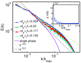
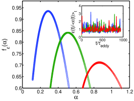
Figure 4: (Color online) Log-log plots (base $10$) versus the scaled wavenumber $k/k_{max}$ of (a) $E(k)$ for runs R2 ($\langle d_{p}\rangle_{t}/L=0.324$, deep-blue line with asterisks), R12 ($\langle d_{p}\rangle_{t}/L=0.22$, green line with crosses), R16 ($\langle d_{p}\rangle_{t}/L=0.177$, red line with circles), R20 ($\langle d_{p}\rangle_{t}/L=0.126$, light-blue line with plus signs), and R1 (single-phase fluid, magenta line); the power-laws $k^{-3.6}$ and $k^{-5.2}$ are depicted by yellow-dash-dot and black-dashed lines, respectively; (b) $E(k)$ for runs R7 ($\langle d_{p}\rangle_{t}/L=0.22$, $We=5.34$, green line with circles) and a 2D Navier-Stokes run with a single-phase fluid, but with a viscosity of $\nu_{eff}(k)=\nu+\Delta\nu(k)$ (blue line with circles); (c) plots of $\langle Re_{\lambda}\rangle_{t}$ versus $\sigma$ for the runs R7-R14 ($\langle d_{p}\rangle_{t}/L=0.22$) (the inset shows $\langle Re_{\lambda}\rangle_{t}$ versus $\langle d_{p}\rangle_{t}/L$ for the runs R2-R6, R12 and R16-R20 ($\sigma=0.069$ or $We=1.38$)); (d) the multifractal spectrum $f_{\varepsilon}(\alpha)$ versus $\alpha$ of the normalized energy-dissipation rate $\varepsilon(t)$ versus $t$ for $\langle d_{p}\rangle_{t}/L=0.324$ (R2, blue circles), $\langle d_{p}\rangle_{t}/L=0.15$ (R20, green squares) and single-phase fluid turbulence (R1, red diamonds); the inset shows the corresponding normalized energy-dissipation rate $\varepsilon(t)$ versus $t$ for the same runs; the order-parameter spectrum $S(k)=|\hat{\phi}(k)|^{2}$ for the runs (e) R7 ($We=5.34$, deep-blue line with circles) and R13 ($We=0.534$, green line with circles) at $\langle d_{p}\rangle_{t}/L=0.22$; the insets show pseudocolor plots of $\phi$ with dotted arrows indicating the corresponding $We$ and (f) R12 ($\langle d_{p}\rangle_{t}/L=0.22$, deep-blue line with circles) and R20 ($\langle d_{p}\rangle_{t}/L=0.126$, green line with circles); the insets show pseudocolor plots of $\phi$.

IV IV. CONCLUSIONS

Our extensive DNS of the 2D CHNS equations (1)-(2) shows that the two-way coupling between the droplet and the background phase yields very interesting results: The fluid turbulence leads to rich, multifractal fluctuations in the droplet shape. Furthermore, the droplet motion modifies $E(k)$ in two important ways : (a) oscillations with period $\simeq 2\pi/\langle d_{p}\rangle_{t}$ appear; (b) and the large-$k$ tail of $E(k)$ is enhanced relative to that in single-fluid NS turbulence. This enhancement can be rationalized in terms of the scale-dependent viscosity $\nu_{eff}(k)$, which results in dissipation reduction. By using soap-film experiments, Ref. solomon98 has investigated droplet breakup in two-dimensional chaotic flows. Similar experiments in the turbulent regime should be able to verify our predictions of multifractal droplet dynamics, droplet-induced modifications of $E(k)$, and the dissipation reduction that follows from the enhancement of the large-$k$ tail of $E(k)$.

Drag reduction by bubbles occurs in wall-bounded turbulent flows Trigvason2004 ; it has also been studied in the limit of minute bubbles proc2005 . We show that, even at the level of a single droplet with a diameter in inertial-range scales, we obtain the bulk analog of drag reduction, namely, dissipation reduction in homogeneous, isotropic turbulence. Furthermore, the analog of the large-$k$ enhancement in $E(k)$, which we find here, has been seen in three-dimensional experiments in turbulent bubbly flows lohse06 ; prakash13 ; mendez13 .

Although the CHNS approach has been used to study droplet dynamics in a laminar prosperetti2014 ; bifarale2014 ; prakash2015 flow, wall-drag of a droplet in a turbulent channel flow scarbolo2015a , droplet breakup or coalescence scarbolo2015 , steady-state droplet-size distributions perlekar12 ; skartlien13 , and the turbulence-induced arrest of phase separation perlekar2014 , it has neither been used to study droplet fluctuations and droplet-acceleration statistics, in a turbulent flow, nor the modification of fluid turbulence by droplet fluctuations because of the two-way coupling, which we investigate. These issues have also not been considered by other DNSs of drag reduction in channel flows xu2002 , boundary layers ferrante99 ; jacob2010 , and in some experiments hassan2002 ; fontainne99 with droplets.

V APPENDIX

In the main part of this paper we have presented results for $Gr=3\times 10^{7}$. We show now that these results are qualitatively unchanged when we increase $Gr$ to, say, $Gr=1.5\times 10^{8}$. Consider, e.g., the illustrative plot of $P(a_{y})$ versus $a_{y}$ for $Gr=1.5\times 10^{8}$ that we show in Fig. 5(a). This is qualitatively similar to Fig. 3(b) for $Gr=3\times 10^{7}$. In Fig. 5(b) we show the plots of $\langle a_{rms}\rangle_{t}$ versus $\langle d_{p}\rangle_{t}/L$ for $Gr=3\times 10^{7}$ and $Gr=1.5\times 10^{8}$; although the curve for $Gr=1.5\times 10^{8}$ lies well above that for $Gr=3\times 10^{7}$.

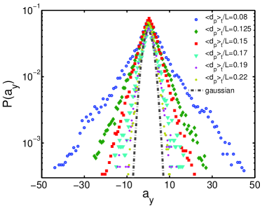
Figure 5: (Color online)(a) Semilog (base $10$) plots of the PDFs $P(a_{y})$, the PDF of $a_{y}$ of the center of mass of the droplets for runs R28 ($\langle d_{p}\rangle_{t}/L=0.126$, deep-blue circles), R27 ($\langle d_{p}\rangle_{t}/L=0.153$, green diamonds), R26 ($\langle d_{p}\rangle_{t}/L=0.22$, red squares), R25 ($\langle d_{p}\rangle_{t}/L=0.263$, light-blue downward-pointing triangles), R24 ($\langle d_{p}\rangle_{t}/L=0.283$, magenta plus signs) and R23 ($\langle d_{p}\rangle_{t}/L=0.32$, yellow asterix) at $We=0.138$ (these PDFs are not scaled by their rms values); (b) log-log (base $10$) plot $\langle a_{rms}\rangle_{t}$, the root-mean square acceleration of the droplet center of mass, versus $\langle d_{p}\rangle_{t}/L$.

In the multifractal spectrum calculation, we use a Wavelet Transform Modulus Maxima Method. The wavelet transform of a function $f$ decomposes it into several elementary wavelets, which are all constructed from a single the analysing wavelet $\psi$. This transform is defined as follows:

$$T_{\psi}[f](x,a)=\frac{1}{a}\int\limits_{-\infty}^{+\infty}\psi(\frac{x-b}{a})f(x)dx,$$ (21)

where $a\in\mathcal{R}$ is a scale parameter and $b\in\mathcal{R}$ is a space parameter; structures smaller than $a$ are smoothed out; and the wavelet $\psi$ is invariant under spatial shifts of length $b$. At each scale $a$, we pick the local maxima of $|T_{\psi}f(x,a)|$ and define the following partition function:

$$Z(a,q)=\sum\limits_{l\in\mathcal{L}(a)}\left(\sup_{(x,a^{\prime})\in l}|T_{\psi}f(x,a^{\prime})|\right)^{q},$$ (22)

where $q\in\mathcal{R}$. In the limit $a\rightarrow 0$, the Renyi exponents $\tau(q)$ follow from

$$Z(a,q)\sim a^{\tau(q)};$$ (23)

the following Legendre transform of $\tau(q)$ yields the multifractal spectrum

$$f(\alpha)=\min_{\alpha}[q\alpha-\tau(q)],$$ (24)

where $\alpha=d\tau(q)/dq$. In our calculations we follow Ref. muzy1993 ; in particular, we use a slightly modified version of the computer program given in Refs. ashken ; physionet . In our calculations, the analyzing wavelet is a Gaussian function. We obtain partition functions $Z(a,q)$ between moments $q_{max}$ and $q_{min}$, with resolution $dq$, $q_{max}=2.0$, $q_{min}=-2.0$, and $dq=0.2$. The value of $a$ is $L_{s}/8$, where $L_{s}$ is the signal length.

References

- (1) J. Bec, L. Biferale, G. Boffeta , A. Celani, M. Cencini , A. Lanotte , S. Musacchio and F. Toschi, J. Fluid Mech., 550, 349-358 (2006).
- (2) W. W. Grabowski and L.P. Wang, Annu. Rev. Fluid Mech. 45, 293-324, (2013).
- (3) R. A. Shaw, Annu. Rev. Fluid Mech. 35.1, 183-227 (2003).
- (4) C.A. Chryssakis, D. Assanis, J. Lee and K. Nishida, No. 2003-01-0007, SAE Technical Paper, 2003.
- (5) C. N. Baroud, F. Gallaire, and R. Dangla, Lab on a Chip 10, 2032-2045 (2010).
- (6) A van der Bos, M J van der Meulen, T. Driessen, M van den Berg, H. Reinten, H. Wijshoff, M. Versluis, and D. Lohse, Phys. Rev. Applied 1, 014004 (2014).
- (7) I.M. Mazzitelli, D. Lohse and F. Toschi, Phys. Fluids 15, L5-L8 (2003).
- (8) L. Biferale, G. Boffeta, A. Celani, A. Lanotte, and F. Toschi, Phys. Fluids 17 021701 (2005).
- (9) P. M. Chaikin and T. C. Lubensky, Principles of Condensed Matter Physics (Cambridge University Press, Reprint edition (2000)) .
- (10) P.C. Hohenberg and B. I. Halperin, Rev.Mod. Phys 49 435 (1977).
- (11) I. M. Lifshitz and V. V. Slyozov, J. Phys. Chem. Solids 19, 35 (1959); H. Furukawa, Phys. Rev. A 31, 1103 (1985); E. D. Siggia, Phys. Rev. A 20, 595 (1979);
- (12) J.D. Gunton, M. San Miguel, and P.S. Sahni, in Phase Transitions and Critical Phenomena, eds. C. Domb and J.L. Lebowitz, Vol. 8 (Academic, London, 1983).
- (13) A. J. Bray, Adv. Phys., 43, 357-459, 1994.
- (14) J. Lothe and G.M. Pound, J. Chem. Phys. 36, 2080 (1962).
- (15) A. Onuki, Phase Transition Dynamics (Cambridge University Press, UK, 2002).
- (16) V. E. Badalassi, H. D. Ceniceros, and S. Banerjee, J. Comput. Phys. 190, 371–397 (2003).
- (17) P. Perlekar, R. Benzi, H. J. H. Clercx, D. R. Nelson and F. Toschi, Phys. Rev. Lett, 112, 014502 (2014).
- (18) J.W. Cahn, Acta metall 9, 795 1961.
- (19) S. Berti, G. Boffetta, M. Cencini and A. Vulpiani, Phys. Rev. Lett. 95, 224501 (2005). A.J. Wagner and J. M. Yeomans, Phys. Rev. Lett. 80, 1429 (1998); V.M. Kendon, Phys. Rev. E, 61, R6071 (R) (2000); V.M. Kendon, M.E. Cates, I.P. Barraga, J.C. Desplat, P. Blandon, J. Fluid Mech., 440, 147 (2001); S. Puri, in Kinetics of Phase Transitions, eds. S. Puri and V. Wadhawan (CRC Press, Boca Raton, US, 2009), Vol. 6, p. 437.
- (20) G. Boffetta and R. Ecke, Annu. Rev Fluid Mech. 44, 427-451 (2012); R. Pandit, P. Perlekar, and S. S. Ray, Pramana-Journal of Physics, 73, 157(2009).
- (21) P. Perlekar, S. S. Ray, D. Mitra and R. Pandit, Phys. Rev. Lett. 106, 054501 (2011).
- (22) R. Fjørtoft, Tellus 5, 226 (1953).
- (23) R. H. Kraichnan, Phys. Fluids 10, 1417 (1967).
- (24) C. Leith, Physics of Fluids 11, 671 (1968).
- (25) G. K. Batchelor, Phys. Fluids Suppl. II 12, 233 (1969).
- (26) M. Lesieur, Turbulence in Fluids, Vol. 84 of Fluid Mechanics and Its Applications (Springer, The Netherlands, 2008)
- (27) H. Homann and J. Bec, J. Fluid Mech., 651, 81-91 (2010).
- (28) N.M. Qureshi, M. Bourgoin, C. Baudet, A. Cartellier, Y. Gagne, Phys. Rev. Lett. 99, 184502 (2007).
- (29) R. J. Hill and J.M. Wilczak, J. Fluid Mech., 296, 247–269 (1995).
- (30) C. Kalelkar, R. Govindarajan, and R. Pandit, Phys. Rev. E 72, 017301 (2005).
- (31) P. Perlekar, D. Mitra, and R. Pandit, Phys. Rev. Lett. 97, 264501 (2006); W.H.Cai, F.C.Li and H.N. Zhang, J. Fluid Mech. 665 334 (2010).
- (32) A. Gupta, P. Perlekar, R. Pandit, Phys. Rev. E 91(3), 033013 (2015).
- (33) A. Celani, A. Mazzino, P. Muratore–Ginanneschi and L. Vozella, J.Fluid Mech., 622, 115-134 (2009).
- (34) L. Scarbolo and A. Soldati, J. Turb. 14, 11 (2013).
- (35) P. Yue, J.J. Feng, C. Liu, and J. Shen, J. Fluid Mech. 515, 293-317 (2004).
- (36) L. Scarbolo, D. Molin and A. Soldati, APS Division of Fluid Dynamics Meeting Abstracts. 1, 4002 (2011).
- (37) S. Childress, R.R. Kerswell and A.D. Gilbert, Physica D 158, 105-128 (2001).
- (38) C. Canuto, M. Y. Hussaini, A. Quarteroni, and T. A. Zang, Spectral Methods in Fluid Dynamics, Springer.
- (39) S. M. Cox, and P. C. Matthews, J. Comput. Phys. 176, 430-455 (2002).
- (40) http://www.nvidia.com/object/cudahomenew.html.
- (41) P. Perlekar, L. Biferale, M. Sbragaglia, S. Srivastava, and F. Toschi, Phys. Fluids 24, 065101 (2012).
- (42) https://www.youtube.com/watch?v=p-lXR9VRcjI&feature=youtu.be. https://www.youtube.com/watch?v=DxspQUL46pU&feature=youtu.be.
- (43) J. F. Muzy, E. Bacry, and A. Arneodo, Phys. Rev. E 47, 875 (1993).
- (44) https://www.physionet.org/physiotools/multifractal
- (45) A.L. Goldberger, L.A.N Amaral, L. Glass, J.M. Hausdorff, Pch Ivanov, R.G. Mark, J.E. Mietus, G.B. Moody, C-K Peng, H.E. Stanley, PhysioBank, PhysioToolkit, and PhysioNet, Components of a New Research Resource for Complex Physiologic Signals. Circulation 101:e215-e220 [Circulation Electronic Pages; http://circ.ahajournals.org/cgi/content/full/101/23/e215]; 2000.
- (46) L. Biferale, P. Perlekar, M. Sbragaglia, S. Srivastava, and F. Toschi, J. Phys.: Conf. Ser. 318, 052017 (2011).
- (47) Even in the 3D studies of Refs.jeremie ; qureshi2007 , the power-law ranges are small.
- (48) In the absence of this droplet, our forcing scheme yields a fluid-energy spectrum that is dominated by a forward cascade of the enstrophy.
- (49) P. Perlekar and R. Pandit, New J. Phys., 11, 073003 (2009).
- (50) G. Boffetta and R. E. Ecke, Annu. Rev. Fluid Mech. 44, 427 (2012).
- (51) T. H. Solomon, S. Tomas, and J. L. Warner, Phys. Fluids 10, 342 (1998).
- (52) J. Lu, and Gretar Tryggvason, APS Division of Fluid Dynamics Meeting Abstracts, 1 (2004).
- (53) V. S. Lv̀ov, A. Pomyalov, I. Procaccia, and V. Tiberkevich, Phys. Rev. Lett. 94, 174502 (2005).
- (54) T. H. Van Den Berg, S. Luther, I. M. Mazzitelli, J. M. Rensen, F. Toschi and D. Lohse, Journal of Turbulence 7, No. 14, 2006.
- (55) V.N. Prakash, J.M. Mercado, F.E.M. Ramos, Y. Tagawa, D. Lohse and C. Sun, arXiv preprint arXiv:1307.6252 (2013).
- (56) S. Mendez-Diaz, J. C. Serrano-Garcia, R. Zenit, and J. A. Hernandez-Cordero, Phys. Fluids, 25, 043303 (2013).
- (57) B. Ray and A. Prosperetti, Chemical engineering science 108, 213-222 (2014).
- (58) L. Biferale, C. Meneveau and R. Verzicco, J. Fluid Mech. 754, 184–207 (2014).
- (59) N.J. Cira, A. Benusiglio, and M. Prakash, Nature 519, 446–450 (2015).
- (60) L. Scarbolo, A. Soldati, Comput. Fluids 113, 87-92 (2015).
- (61) L. Scarbolo, F. Bianco, A. Soldati, Phys. Fluids 27, 073302 (2015).
- (62) R. Skartlien, E. Sollum, H. Schumann, J. Chem. Phys. 139, 174901 (2013).
- (63) J. Xu, M. Maxey and G. Karniadakis, J. Fluid Mech. 468, 271–281 (2002).
- (64) A. Ferrante and S. Elghobashi, J. Fluid Mech. 503, 345 (1999).
- (65) B. Jacob, A. Olivieri, M. Miozzi, E. F. Campana, and R. Piva, Phys. Fluids 22, 115104 (2010).
- (66) Y.A. Hassan and J. Ortiz-Villafuerte, In Proceedings 11th Int. Symp. Applications of Laser Techniques to Fluid Mechanics Lisbon, July 8-11, (Paper 23.3), (2002).
- (67) A.A. Fontaine, S. Deutsch, T.A. Brungart, H.L. Petrie and M. Fenstermacker, Exp. Fluids, 26 397–403 (1999).