Anomalous dimensions on the lattice

Joel Giedt

Department of Physics, Applied Physics and Astronomy
Rensselaer Polytechnic Institute, 110 8th Street, Troy, NY 12180 USA

We review methods and results for extracting the anomalous dimensions of operators from lattice field theory calculations. The most important application is the anomalous mass dimension in conformal or nearly conformal gauge field theories which might be related to dynamical electroweak symmetry breaking. Some discussion of the underlying theory of renormalization and mixing of operators is also included.

1 Introduction

The fact that composite operators in an interacting quantum field theory do not have the naive, classical scaling dimension associated with the Gaussian fixed point, but actually have a quantum mechanical dimension, which includes a so-called “anomalous” part, is well known [1, 2]. (Anomalous dimensions were anticipated in earlier work on critical phenomena, such as [3].) In some cases, the interacting theory is solvable and one can compute these dimensions exactly. However, that is rarely the case. In other cases, supersymmetry and conformal symmetry are present and the superconformal algebra relates the scaling dimension to the charge under the $U(1)_{R}$ symmetry, so that at least in the case of “chiral” operators the anomalous dimension is known exactly. Another avenue is that the theory is weakly coupled, so that one can compute the anomalous dimension in a perturbative approximation; this would be true, for instance, in the case of a Banks-Zaks fixed point [4]. Nonperturbative approaches must be used when the theory is strongly coupled, as in an asymptotically free theory that is far away from the Banks-Zaks limit. One can use truncated Schwinger-Dyson equations to derive estimates of the anomalous dimension, but this is an uncontrolled approximation. Ultimately one would like to obtain the nonperturbative estimate to arbitrary accuracy using a first principles approach with a controlled approximation that can be systematically improved. Lattice gauge theory provides a tool to obtain such an estimate, but it is fraught with technical and practical difficulties, as will be made clear in this report. Nevertheless, it is a route that is worth pursuing in the case where exact methods are unavailable and the theory is strongly interacting.

Several groups have recently computed the anomalous mass dimension, essentially the scaling dimension of the scalar fermion bilinear operator ${\cal O}_{S}={\bar{\psi}}\psi$, in theories that are cousins of massless QCD: fermions coupled to a nonabelian gauge field, in the chiral limit (where the current “quark” mass is zero). The interest in this topic has been motivated by the desire to find viable models of walking technicolor (TC), where a large anomalous mass dimension leads to condensate enhancement,

$$\langle{\bar{\psi}}\psi\rangle_{\text{ETC}}\sim\left(\frac{\Lambda_{\text{ETC}}}{\Lambda_{\text{TC}}}\right)^{\gamma_{*}}\langle{\bar{\psi}}\psi\rangle_{\text{TC}}$$ (1.1)

which is important for the suppression of flavor-changing neutral currents. These flavor changing processes are mediated by the exchange of extended technicolor (ETC) gauge bosons, and the mass scale of these particles needs to be high in order to avoid constraints from experimental flavor physics. On the other hand, such a high scale would also naively suppress the fermion masses of the standard model. This is avoided if the technicolor condensate that feeds into the fermion masses is enhanced, due to a large anomalous dimension—an explicit mathematical formulation of this will be given below. In practice one desires $\gamma_{*}\approx 1$ for viable phenomenology [5]. Thus the lattice community has been examining the anomalous mass dimension in various theories that might serve as walking technicolor candidates, as well as theories that are more QCD like in order to draw a contrast. Several techniques for doing this have been exploited and developed. In this report we will describe most of the methods that have been used to date, and will attempt to compare them in terms of their reliability and efficacy.

The walking technicolor motivation for such studies is under stress from the recent discovery of the Higgs boson, which appears to have all of the properties of the minimal elementary scalar field model. In fact, even two Higgs doublet models such as appear in supersymmetric extensions seem to be forced into the decoupling limit where the CP odd Higgs scalar $A^{0}$ is very heavy. Naively one might think that the lightest scalar in a technicolor theory should be heavy. After all in QCD the $\sigma$ resonance is of order 500 MeV, which is quite a bit larger than the pion decay constant $f_{\pi}\sim 90$ MeV. In the technicolor model, the pion decay constant is scaled up to the Higgs vacuum expectation value, $v=f_{\pi}=246$ GeV, so one would expect the analogue of the $\sigma$ to be of order 1 TeV, not the 125 GeV of the observed Higgs boson. However, it has recently been pointed out that electroweak corrections, principally the top quark loop, have the right sign and magnitude to bring the mass of the $\sigma$ down significantly, possibly even to 125 GeV [10], if the $\sigma$ is perhaps a bit lighter than scaled up QCD would predict. A somewhat light $\sigma$ may happen in walking technicolor because the dynamics is significantly different and there is an approximate zero of the $\beta$ function at some scale, which some have argued can suppress the mass of the lightest scalar (the so-called techni-dilaton).

The lattice studies have for the most part found $\gamma\mathrel{\hbox to0.0pt{\raise 2.15277pt\hbox{$<$}\hss}{\lower 2.15277pt\hbox{$\sim$}}}0.5$, which is too small for the walking scenario. However, there is the potential to solve this problem with the four-fermion terms that will be induced by extended technicolor [11]. This may also be used to push a theory out of the conformal window, so that it really is walking. For this reason, detailed lattice studies of theories with four-fermion terms in the action need to be pursued in the future. This is not a simple matter since introducing four-fermion terms often destroys the positivity of the fermion measure, leading to an apparently insurmountable sign problem. Nevertheless, a judicious choice of theory and lattice discretization can avoid this problem and would lead to very interesting results if studied in light of the proposal implied by [11].

Apart from technicolor type models, anomalous dimensions and conformal fixed points are important problems for a variety of reasons. In some supersymmetric theories the hidden sector may be nearly conformal and the anomalous dimension of some operators can determine the impact of the hidden sector on soft parameters; this can be significant. Simply knowing the sign of the anomalous dimension of some operators can give answers to qualitative questions. Of course one would also have to solve the supersymmetry problem on the lattice in order to conduct such a study.

Knowledge of the running of the anomalous dimension in asymptotically free gauge theories has also played a role in holographic calculations [12]. In that context the running of $\gamma$ translates into a mass-squared for the scalar dual to ${\bar{q}}q$ that depends on the AdS radius, $m^{2}=m^{2}(r)$. Here it is interesting that the Breitenlohner-Freedman bound occurs precisely when $\gamma=1$, the number which is sought after in the lattice gauge theory studies. Such a value may indeed occur near the critical number of flavors, such as $N_{c}=3$ with $N_{f}=10$ fundamental representation fermions [13], or $N_{c}=2$ with $N_{f}=1$ adjoint Dirac fermions [14].

2 Anomalous dimensions

Correlation functions of the bare fields $\phi_{0}$ and bare operators ${\cal O}_{0}$ require renormalization in order to obtain finite answers:

$$\langle 0|\phi(x_{1})\cdots\phi(x_{n}){\cal O}(y)|0\rangle=Z_{\cal O}Z_{\phi}^{-n/2}\langle 0|\phi_{0}(x_{1})\cdots\phi_{0}(x_{n}){\cal O}_{0}(y)|0\rangle$$ (2.1)

That this even works to render the left-hand side finite is in itself amazing: an infinite number of correlation functions (taking all possible choices of $n$) are renormalized just using two renormalization constants $Z_{\phi}$ and $Z_{\cal O}$ (of course the bare masses and couplings will also need to be adjusted to cancel the infinities, but for a renormalizable theory this is a finite set). The $Z$ factors depend on the renormalization scale $\mu$. In particular,

$${\cal O}(\mu;y)=Z_{\cal O}(\mu){\cal O}_{0}(y)$$ (2.2)

The $Z$ factor for the operator satisfies a renormalization group equation,

$$\gamma_{\cal O}(g(\mu))=-\frac{d}{d\ln\mu}\ln Z_{\cal O}(\mu)$$ (2.3)

where we show explicitly that the anomalous dimension $\gamma_{\cal O}$ is a function of the running coupling $g(\mu)$. Since the bare operator is independent of the renormalization scale $\mu$,

$$\frac{d}{d\ln\mu}{\cal O}(\mu;y)=-\gamma_{\cal O}{\cal O}(\mu;y)$$ (2.4)

These equations ignore the issue of mixing, which is often not negligible. To take this into account, we generalize to a bare operator basis ${\cal O}_{0,i}$ and a renormalized set of operators ${\cal O}_{i}$. Then these are related by

$${\cal O}_{i}(\mu;y)=Z_{ij}(\mu){\cal O}_{0,j}(y)$$ (2.5)

where of course there is a sum over $j$ on the right-hand side. The renormalization group equation generalizes to

$$\frac{d}{d\ln\mu}Z_{ij}(\mu)=-\gamma_{ik}(g(\mu))Z_{kj}(\mu)$$ (2.6)

Contracting with the bare operators, we see then that there is a corresponding flow in the space of renormalized operators,

$$\frac{d}{d\ln\mu}{\cal O}_{i}(\mu;y)=-\gamma_{ik}(g(\mu)){\cal O}_{k}(\mu;y)$$ (2.7)

In the case of the fermion mass operator ${\bar{\psi}}\psi$, since $m{\bar{\psi}}\psi$ is RG invariant (it appears in the trace of the energy momentum tensor, a conserved current), the anomalous dimension of this operator is also related to the dimension of the mass:

$$\gamma_{{\bar{\psi}}\psi}=\gamma_{m}=-\frac{d\ln m}{d\ln\mu}$$ (2.8)

The operators will have a canonical, or engineering, dimension

$$[{\cal O}_{i}]=d_{i}$$ (2.9)

Up to ${{\cal O}(a)}$ terms, the operators will only mix with those of the same dimension or lower. This then takes the form

$${\cal O}_{i}(\mu;x)=\sum_{j\in S}a^{-d_{i}+d_{j}}C_{ij}(\mu a){\cal O}_{0,j}(x)+{{\cal O}(a)}$$ (2.10)

where $S$ is the set of operators with $d_{j}\leq d_{i}$. The operators of dimension $d_{j}<d_{i}$ do not affect the anomalous dimensions of the operators of dimension $d_{i}$ [15]. Nevertheless, they play an important role, for instance in the determination of counterterms to restore symmetries; see for example [15] for a discussion of axial Ward identities with Wilson fermions, or [16] for supersymmetry Ward identities again with Wilson fermions. The ${{\cal O}(a)}$ terms that are not shown are important in ${{\cal O}(a)}$ improvement. It is quite expensive to reduce the lattice spacing in a lattice simulation because the spatial size $L=Na$ must be kept constant to avoid finite size effects, and the number of degrees of freedom will increase as $1/a^{4}$. In addition, as one reduces the lattice spacing one simulates closer to a second order critical point and so there is a critical slowing down in the algorithms. In practice it is better to first reduce the discretization errors as much as possible. This can be achieved by fine-tuning irrelevant operators in the action and by making ${{\cal O}(a)}$ improvements to operators that are being measured.

The anomalous dimensions of composite operators also make an appearance in a generalization of the Callan-Symanzik equations for renormalized Green functions,

$$\left[\mu\frac{{\partial}}{{\partial}\mu}+\beta(g)\frac{{\partial}}{{\partial}g}+n\gamma(g)+m\gamma_{\cal O}(g)\right]\langle 0|\Phi^{R}(x_{1})\cdots\Phi^{R}(x_{n}){\cal O}^{R}(y_{1})\cdots{\cal O}^{R}(y_{m})|0\rangle=0$$ (2.11)

Here $\Phi^{R}$ represent the renormalized elementary fields. This also provides a rubric for finding the anomalous dimensions from the counterterms $\delta Z_{\cal O}$ which are involved in rendering the Green function

$$G^{R,n,m}(x_{1},\ldots,x_{n};y_{1},\ldots,y_{m})=\langle 0|\Phi^{R}(x_{1})\cdots\Phi^{R}(x_{n}){\cal O}^{R}(y_{1})\cdots{\cal O}^{R}(y_{m})|0\rangle$$ (2.12)

finite. Explicit examples will be considered below.

3 Non-lattice methods

3.1 Perturbation theory

In a theory of only fermions with gauge interactions, the one loop anomalous mass dimension is universal (scheme independent) and given by

$$\left.\gamma_{{\bar{\psi}}\psi}\right|_{\text{1-loop}}=-\frac{3C_{2}(R)\alpha}{2\pi}$$ (3.1)

The minus sign originates from our definition (2.3) with Z being used to obtain the renormalized operator from the bare operator as in (2.2), rather than the other way around. Universality is easily seen, since it would correspond to a redefinition $\alpha\to\alpha+{{\cal O}(\alpha^{2})}$, which will not affect the one-loop result.

The two-loop contribution in the MS or $\overline{\text{MS}}$ schemes is given by

$$\left.\gamma_{{\bar{\psi}}\psi}\right|_{\text{2-loop}}=-\frac{C_{2}(R)\alpha^{2}}{16\pi^{2}}\left(\frac{203}{6}N_{c}-\frac{3}{2N_{c}}-\frac{10}{3}N_{f}\right)$$ (3.2)

Also in these schemes the three and four loop results are known and given in Refs. [17, 18].

3.2 Unitarity bounds

Unitarity constraints on the conformal group [19] imply that $\gamma_{*}\leq 2$. For supersymmetric theories, further constraints exist, as studied extensively in [20] and reviewed in [21]. Thus in general we can use the power of the conformal group, or yet more power of the superconformal group, to extract information about the scaling dimensions. Of course, this requires that the theory be conformal. A necessary, but not always sufficient condition, is that it be scale invariant. However, as pointed out in [20], a quantum field theory must include a cutoff, and a scale transformation scales the cutoff. So if there is any cutoff dependence in the quantum theory, say $\Lambda dg/d\Lambda=\beta(g)\not=0$, then the theory will not be conformally invariant. Hence the need for a vanishing $\beta$ function.

3.3 Example: QED at one loop

Here, we will work in the limit of vanishing electron mass. As will be seen, this also corresponds to a mass independent scheme for subtracting the infinities.

Figure 1: The cross denotes the operator insertion. In the case of bare perturbation theory, $\delta Z_{{\bar{\psi}}\psi}-\delta Z_{\psi}$ times the tree level diagram must cancel the loop divergences of the other three diagrams. In the case of renormalized perturbation theory, the divergences will be cancelled by counterterms that are shown in Fig. 2 below.

3.3.1 Bare perturbation theory

Our first approach will be to use bare perturbation theory with dimensional regularization. Then the finite Green function is obtained from the bare one according to

$$\langle 0|T{\bar{\psi}}\psi(x)\psi(y){\bar{\psi}}(z)|0\rangle=Z_{{\bar{\psi}}\psi}Z_{\psi}^{-1}\langle 0|T{\bar{\psi}}_{0}\psi_{0}(x)\psi_{0}(y){\bar{\psi}}_{0}(z)|0\rangle$$ (3.3)

We will work to order $e^{2}$, and then writing $Z_{\psi}=1+\delta Z_{\psi}$ and $Z_{{\bar{\psi}}\psi}=1+\delta Z_{{\bar{\psi}}\psi}$ this formula becomes

$$\langle 0|T{\bar{\psi}}\psi(x)\psi(y){\bar{\psi}}(z)|0\rangle=\langle 0|T{\bar{\psi}}_{0}\psi_{0}(x)\psi_{0}(y){\bar{\psi}}_{0}(z)|0\rangle_{tree}$$

$$\qquad+\langle 0|T{\bar{\psi}}_{0}\psi_{0}(x)\psi_{0}(y){\bar{\psi}}_{0}(z)|0\rangle_{1-loop}$$

$$\qquad+(\delta Z_{{\bar{\psi}}\psi}-\delta Z_{\psi})\langle 0|T{\bar{\psi}}_{0}\psi_{0}(x)\psi_{0}(y){\bar{\psi}}_{0}(z)|0\rangle_{tree}$$ (3.4)

Thus the infinities in the 1-loop term must be subtracted off by corresponding infinite values of $\delta Z_{{\bar{\psi}}\psi}$ and $\delta Z_{\psi}$. The tree diagram is shown in the first diagram of Fig. 1 and the 1-loop diagrams are shown in the other diagrams of Fig. 1. On the other hand, $\delta Z_{\psi}$ is independently determined by the self energy calculation

$$\langle 0|T\psi(y){\bar{\psi}}(z)|0\rangle=Z_{\psi}^{-1}\langle 0|T\psi_{0}(y){\bar{\psi}}_{0}(z)|0\rangle$$

$$\qquad=\langle 0|T\psi_{0}(y){\bar{\psi}}_{0}(z)|0\rangle_{tree}+\langle 0|T\psi_{0}(y){\bar{\psi}}_{0}(z)|0\rangle_{1-loop}$$

$$\qquad\qquad-\delta Z_{\psi}\langle 0|T\psi_{0}(y){\bar{\psi}}_{0}(z)|0\rangle_{tree}$$ (3.5)

Comparing the two calculations, it can be seen that the $-\delta Z_{\psi}$ in (3.4) cancels one of the two self energy corrections show in Fig. 1, but the other is not cancelled, and so contributes to the value of $\delta Z_{{\bar{\psi}}\psi}$. This is because at one loop (3.4) has twice as many self energy corrections as (3.5), but the same factor $Z_{\psi}^{-1}$. The amputated version of the upper right-hand diagram in Fig. 1 will be denoted $\Gamma(q^{2},p^{2},q\cdot p)$, having passed to momentum space. What we have found is that

$$\delta Z_{{\bar{\psi}}\psi}=-\Gamma(\mu)-\delta Z_{\psi}$$ (3.6)

where $\Gamma(q^{2},p^{2},q\cdot p)=\Gamma(-\mu^{2},-\mu^{2},-\mu^{2})\equiv\Gamma(\mu)$ is the subtraction point. What is left is to compute the two terms on the right-hand side.

Amputating the self energy diagram we obtain

$$-i\Sigma(\hbox to0.0pt{\hbox to5.03125pt{\hfil/\hfil}\hss}p) = (-ie)^{2}\int\frac{d^{d}k}{(2\pi)^{d}}\frac{i\gamma_{\mu}(\hbox to0.0pt{\hbox to5.52084pt{\hfil/\hfil}\hss}k+\hbox to0.0pt{\hbox to5.03125pt{\hfil/\hfil}\hss}p)\gamma^{\mu}}{(k+p)^{2}+i{\epsilon}}\frac{-i}{k^{2}+i{\epsilon}}$$ (3.7)

$$= (d-2)e^{2}\int\frac{d^{d}k}{(2\pi)^{d}}\frac{\hbox to0.0pt{\hbox to5.52084pt{\hfil/\hfil}\hss}k+\hbox to0.0pt{\hbox to5.03125pt{\hfil/\hfil}\hss}p}{[(k+p)^{2}+i{\epsilon}][k^{2}+i{\epsilon}]}$$

$$= (d-2)ie^{2}\hbox to0.0pt{\hbox to5.03125pt{\hfil/\hfil}\hss}p\int_{0}^{1}dx~{}(1-x)(4\pi)^{-d/2}\Gamma(2-\frac{d}{2})\Delta^{\frac{d}{2}-2}$$

$$= \frac{ie^{2}}{8\pi^{2}}\hbox to0.0pt{\hbox to5.03125pt{\hfil/\hfil}\hss}p\int_{0}^{1}dx~{}(1-x)(\frac{2}{{\epsilon}}+1-\ln\Delta-\gamma+\ln 4\pi)$$

where $\Delta=-x(1-x)p^{2}$ and $d=4-{\epsilon}$. The subtraction condition arising from (3.5) is

$$\left[-\delta Z_{\psi}\frac{i}{\hbox to0.0pt{\hbox to5.03125pt{\hfil/\hfil}\hss}p}+\frac{i}{\hbox to0.0pt{\hbox to5.03125pt{\hfil/\hfil}\hss}p}(-i\Sigma(\hbox to0.0pt{\hbox to5.03125pt{\hfil/\hfil}\hss}p))\frac{i}{\hbox to0.0pt{\hbox to5.03125pt{\hfil/\hfil}\hss}p}\right]_{\hbox to0.0pt{\hbox to3.52188pt{\hfil/\hfil}\hss}p=i\mu}=0$$ (3.8)

so that we find

$$\delta Z_{\psi}=-\frac{e^{2}}{8\pi^{2}}\int_{0}^{1}dx~{}(1-x)(\frac{2}{{\epsilon}}+1-\ln[x(1-x)\mu^{2}]-\gamma+\ln 4\pi)$$ (3.9)

The quantity that we will actually need is

$$\frac{d}{d\ln\mu}\delta Z_{\psi}=\frac{e^{2}}{8\pi^{2}}$$ (3.10)

Next we consider the amputated diagram that was denoted above as $\Gamma(q^{2},p^{2},q\cdot p)$. It is given by

$$\Gamma(q^{2},p^{2},q\cdot p) = (-ie)^{2}\int\frac{d^{d}k}{(2\pi)^{d}}\gamma_{\mu}\frac{i(\hbox to0.0pt{\hbox to5.52084pt{\hfil/\hfil}\hss}k+\hbox to0.0pt{\hbox to5.00002pt{\hfil$q$\hfil}\hss}/+\hbox to0.0pt{\hbox to5.03125pt{\hfil/\hfil}\hss}p)}{(k+q+p)^{2}+i{\epsilon}}\frac{i(\hbox to0.0pt{\hbox to5.52084pt{\hfil/\hfil}\hss}k+\hbox to0.0pt{\hbox to5.03125pt{\hfil/\hfil}\hss}p)}{(k+p)^{2}+i{\epsilon}}\gamma^{\mu}\frac{-i}{k^{2}+i{\epsilon}}$$ (3.11)

The numerator can be simplified to

$$\gamma_{\mu}(\hbox to0.0pt{\hbox to5.52084pt{\hfil/\hfil}\hss}k+\hbox to0.0pt{\hbox to5.00002pt{\hfil$q$\hfil}\hss}/+\hbox to0.0pt{\hbox to5.03125pt{\hfil/\hfil}\hss}p)(\hbox to0.0pt{\hbox to5.52084pt{\hfil/\hfil}\hss}k+\hbox to0.0pt{\hbox to5.03125pt{\hfil/\hfil}\hss}p)\gamma^{\mu}=4(k+q+p)\cdot(k+p)-{\epsilon}(\hbox to0.0pt{\hbox to5.52084pt{\hfil/\hfil}\hss}k+\hbox to0.0pt{\hbox to5.00002pt{\hfil$q$\hfil}\hss}/+\hbox to0.0pt{\hbox to5.03125pt{\hfil/\hfil}\hss}p)(\hbox to0.0pt{\hbox to5.52084pt{\hfil/\hfil}\hss}k+\hbox to0.0pt{\hbox to5.03125pt{\hfil/\hfil}\hss}p)$$ (3.12)

and the ${{\cal O}({\epsilon})}$ term does not contribute to the singularity, but only to finite parts; therefore, we will not include it in the subtraction and drop it henceforth, denoting the resulting integral with a prime, $\Gamma\to\Gamma^{\prime}$. It is now a simple matter to introduce Feynman parameters and write the integral as

$$\Gamma^{\prime}(q^{2},p^{2},q\cdot p) = 8e^{2}\int_{0}^{1}dx\int_{0}^{1-x}dy\int\frac{d^{d}{\tilde{\ell}}}{(2\pi)^{d}}\frac{{\tilde{\ell}}^{2}+{\tilde{\Delta}}}{({\tilde{\ell}}^{2}+\Delta)^{3}}$$ (3.13)

where $\ell=k+xq+(x+y)p$ is a shifted integration momentum, ${\tilde{\ell}}$ is this momentum Wick rotated,

$$\Delta = -x(1-x)q^{2}-(x+y)(1-x-y)p^{2}-2x(1-x-y)p\cdot q$$

$${\tilde{\Delta}} = -x(1-x)q^{2}-(1-x-y)^{2}p^{2}+(1-2x)(1-x-y)p\cdot q$$ (3.14)

The term involving ${\tilde{\Delta}}$ is again finite, we drop it and denote the remaining integral by a double-prime, wich evaluates to

$$\Gamma^{\prime\prime}(q^{2},p^{2},q\cdot p)=\frac{e^{2}}{2\pi^{2}}\int_{0}^{1}dx\int_{0}^{1-x}dy\left(\frac{2}{{\epsilon}}-\gamma-\frac{1}{2}-\ln\Delta+\ln 4\pi\right)$$ (3.15)

Evaluating at the subtraction point $\Gamma^{\prime\prime}(q^{2},p^{2},q\cdot p)=\Gamma^{\prime\prime}(-\mu^{2},-\mu^{2},-\mu^{2})\equiv\Gamma(\mu)$, we obtain

$$\frac{d}{d\ln\mu}\Gamma(\mu)=-\frac{e^{2}}{2\pi^{2}}$$ (3.16)

Finally, taking into account (3.6),

$$\gamma_{{\bar{\psi}}\psi}=-\frac{d}{d\ln\mu}\delta Z_{{\bar{\psi}}\psi}=\frac{d}{d\ln\mu}[\Gamma(\mu)+\delta Z_{\psi}]=-\frac{e^{2}}{2\pi^{2}}+\frac{e^{2}}{8\pi^{2}}=-\frac{3e^{2}}{8\pi^{2}}$$ (3.17)

Thus we see that the calcuation in bare pertubation theory agrees with (3.1) taking into account that the quadratic Casimir for a U(1) gauge theory with a fermion of unit charge is $C_{2}(R)=1$.

Figure 2: Counterterms that cancel the loop divergences of Fig. 1 in renormalized perturbation theory. Note that there are two self-energy subtractions, in contrast to bare perturbation theory.

3.3.2 Renormalized perturbation theory

It is instructive to repeat this exercise from the point of view of renormalized perturbation theory, since there it has an intimate connection with the Callan-Symanzik equation. It will be seen that we do not have any new integrals to compute—only their interpretation is modified. The additional counterterm diagrams are shown in Fig. 2.

We do not get $\gamma_{{\bar{\psi}}\psi}$ directly from (2.3), but rather from the Callan-Symanzik equation

$$\left(\mu\frac{{\partial}}{{\partial}\mu}+\beta(g)\frac{{\partial}}{{\partial}g}+2\gamma_{\psi}+\gamma_{{\bar{\psi}}\psi}\right)G^{(2,1)}(p,q)=0$$ (3.18)

At the one loop level, this reduces to the following equation on the counterterms:

$$\mu\frac{{\partial}}{{\partial}\mu}\delta_{Z_{{\bar{\psi}}\psi}}+2\mu\frac{{\partial}}{{\partial}\mu}\delta_{Z_{2}}+2\gamma_{\psi}+\gamma_{{\bar{\psi}}\psi}=0$$ (3.19)

On the other hand, the Callan-Symanzik equation for the two point function

$$\left(\mu\frac{{\partial}}{{\partial}\mu}+\beta(g)\frac{{\partial}}{{\partial}g}+2\gamma_{\psi}\right)G^{(2)}(p)=0$$ (3.20)

yields

$$\mu\frac{{\partial}}{{\partial}\mu}\delta_{Z_{2}}+2\gamma_{\psi}=0$$ (3.21)

Using this to eliminate the anomalous dimension $\gamma_{\psi}$ of the elementary field, we obtain

$$\gamma_{{\bar{\psi}}\psi}=-\mu\frac{{\partial}}{{\partial}\mu}\left(\delta_{Z_{{\bar{\psi}}\psi}}+\delta_{Z_{2}}\right)$$ (3.22)

The counterterm $\delta_{Z_{2}}$ cancels both of the infinities from the external leg corrections, so that in this formalism $\delta_{Z_{{\bar{\psi}}\psi}}$ is purely cancelling the divergence of the loop around the operator insertion. Thus we recover what we found in bare perturbation theory: the anomalous mass dimension comes from that loop plus one self-energy loop. We obtain an identical result.

3.3.3 Mass independent scheme

Obviously we could repeat all of the calculations with a nonzero fermion mass $m$. However, what we will now show is that the $Z_{{\bar{\psi}}\psi}$ and $Z_{\psi}$ used in the bare perturbation theory in the massless case work just as well in the massive case, as far as rendering the correlation function finite goes. Thus one arrives at a mass independent scheme for renormalizing the bare correlation function in the massive case. This has generalizations to other calculations of renormalization constants which we shall comment on at the end of this discussion.

Consider the two 1-loop diagrams that had infinities, but now for the massive theory. For instance, we now have

$$\Gamma(q^{2},p^{2},q\cdot p)=$$

$$(-ie)^{2}\int\frac{d^{d}k}{(2\pi)^{d}}\gamma_{\mu}\frac{i(\hbox to0.0pt{\hbox to5.52084pt{\hfil/\hfil}\hss}k+\hbox to0.0pt{\hbox to5.00002pt{\hfil$q$\hfil}\hss}/+\hbox to0.0pt{\hbox to5.03125pt{\hfil/\hfil}\hss}p+m)}{(k+q+p)^{2}-m^{2}+i{\epsilon}}\frac{i(\hbox to0.0pt{\hbox to5.52084pt{\hfil/\hfil}\hss}k+\hbox to0.0pt{\hbox to5.03125pt{\hfil/\hfil}\hss}p+m)}{(k+p)^{2}-m^{2}+i{\epsilon}}\gamma^{\mu}\frac{-i}{k^{2}+i{\epsilon}}$$ (3.23)

The numerator “simplification” now becomes

$$\gamma_{\mu}(\hbox to0.0pt{\hbox to5.52084pt{\hfil/\hfil}\hss}k+\hbox to0.0pt{\hbox to5.00002pt{\hfil$q$\hfil}\hss}/+\hbox to0.0pt{\hbox to5.03125pt{\hfil/\hfil}\hss}p+m)(\hbox to0.0pt{\hbox to5.52084pt{\hfil/\hfil}\hss}k+\hbox to0.0pt{\hbox to5.03125pt{\hfil/\hfil}\hss}p+m)\gamma^{\mu}=$$

$$4(k+q+p)\cdot(k+p)-{\epsilon}(\hbox to0.0pt{\hbox to5.52084pt{\hfil/\hfil}\hss}k+\hbox to0.0pt{\hbox to5.00002pt{\hfil$q$\hfil}\hss}/+\hbox to0.0pt{\hbox to5.03125pt{\hfil/\hfil}\hss}p)(\hbox to0.0pt{\hbox to5.52084pt{\hfil/\hfil}\hss}k+\hbox to0.0pt{\hbox to5.03125pt{\hfil/\hfil}\hss}p)$$

$$-(2-{\epsilon})m(2\hbox to0.0pt{\hbox to5.52084pt{\hfil/\hfil}\hss}k+2\hbox to0.0pt{\hbox to5.03125pt{\hfil/\hfil}\hss}p+\hbox to0.0pt{\hbox to5.00002pt{\hfil$q$\hfil}\hss}/)+dm^{2}$$ (3.24)

where again $d=4-{\epsilon}$. It is now clear that all of the terms proportional to $m$ come with one lower power of the loop momentum and are therefore finite, since the leading integral is log divergent. Similarly the term involving $m^{2}$ is finite. Therefore none of these mass dependent terms are divergent, and they do not require a subtraction in order to make the correlation function finite.

Next we expand the denominator in powers of $m^{2}$. For instance,

$$\frac{1}{(k+q+p)^{2}-m^{2}+i{\epsilon}}=\frac{1}{(k+q+p)^{2}+i{\epsilon}}\left[1+{\cal O}\left(\frac{m^{2}}{(k+q+p)^{2}+i{\epsilon}}\right)\right]$$ (3.25)

Obviously all of the corrections are suppress by additional powers of $1/k^{2}$ and therefore finite, again because the leading integral is log divergent. Thus we reach a similar conclusion that mass dependent terms do not require subtraction.

The same line of argument applies to the self energy calculation because it is also log divergent. We find therefore that expanding in powers of the fermion mass $m$, the mass dependent terms are finite, and the only subtractions that we need are in the mass independent part. As a result we can use the $Z_{{\bar{\psi}}\psi}$ and $Z_{\psi}$ determined from the massless theory to render the massive theory finite. Hence we reach the conclusion that a mass independent renormalization scheme is possible.

The key ingredient here was that the leading divergence is logarithmic, a fact that extends to higher orders by power counting. If we were renormalizing some other operator, and we found loop diagrams with quadratic divergences, then expanding in $m$, the $m^{2}$ term would almost certainly contain a logarithmic divergence. In that case the Z factor for the operator would have to contain a mass dependent term in order to renormalize its correlation functions. Thus it is possible to have a situation where a mass independent scheme cannot be achieved if what one is interested in is the operator renormalization constant in the massive theory. Of course this does not change the fact that it is always possible to write the anomalous dimensions in a mass-independent way, if they are defined through the Callan-Symanzik equation with $m{\partial}/{\partial}m$ essentially counting mass insertions into massless Green’s functions, multiplied by $\gamma_{m}$. For instance see Eq. (4.47) below.

As a specific example, the dimension five operator ${\cal O}_{5}^{a}={\bar{q}}\gamma_{5}\tau^{a}D_{\mu}D^{\mu}q$ has this difficulty, where $q=(u,d)$ are quark fields. In the lattice application in which this arises (explained shortly), the operator is multiplied by the lattice spacing $a$. The leading divergence associated with $a{\cal O}_{5}^{a}$ is then linear and the term proportional to $m$ will be logarithmically divergent. Hence it will require a mass-dependent subtraction. In fact this operator is very interesting to study because it is the one generated from an axial flavor transformation of the action with Wilson quarks, and hence appears in the axial Ward identity

$$\langle{\partial}_{\mu}J_{5\mu}^{a}(x){\cal O}(y)\rangle=\langle a{\cal O}_{5}^{a}(x){\cal O}(y)\rangle$$ (3.26)

The mass dependent renormalization of this operator in fact is responsible for the multiplicative renormalization proportional to the bare mass, whereas the linear divergence is responsible for the additive renormalization: $m_{r}=Z_{m}(m_{0}-m_{c})$ with $m_{c}\sim 1/a$ and $Z_{m}\sim\ln a$.

3.4 Dilatation Ward identities

The anomalous dimension is associated with scale transformations; thus it is useful to review the associated Ward identities. The scale transformation ($x\to\lambda x$) of a field is given by

$$\Phi(x)\to\Phi^{\prime}(x)=\lambda^{-\Delta}\Phi(x/\lambda)$$ (3.27)

The infinitesmal form is obtained by taking $\lambda=1+{\epsilon}$ with ${\epsilon}\ll 1$:

$$\delta\Phi(x)=-{\epsilon}(\Delta+x^{\mu}{\partial}_{\mu})\Phi(x)$$ (3.28)

The global form of the Ward identity is obtained from the path integral by taking ${\epsilon}=$ const., using the identity (change of variables of integration invariance)

$$\int[d\Phi]e^{-S[\Phi]}\Phi_{1}(x_{1})\cdots\Phi_{n}(x_{n})=\int[d\Phi^{\prime}]e^{-S[\Phi^{\prime}]}\Phi^{\prime}_{1}(x_{1})\cdots\Phi^{\prime}_{n}(x_{n})$$ (3.29)

with $\Phi^{\prime}_{i}=\Phi_{i}+\delta\Phi_{i}$ and expanding in ${\epsilon}$ to linear order, since ${\epsilon}$ is infinitesmal. Assuming that the action and measure are invariant under the scale transformation

$$[d\Phi^{\prime}]=[d\Phi],\quad S[\Phi^{\prime}]=S[\Phi]$$ (3.30)

this yields

$$\int[d\Phi]e^{-S[\Phi]}\Phi_{1}(x_{1})\cdots\Phi_{n}(x_{n})=\int[d\Phi]e^{-S[\Phi]}\Phi_{1}(x_{1})\cdots\Phi_{n}(x_{n})$$

$$\qquad-{\epsilon}\int[d\Phi]e^{-S[\Phi]}\sum_{i}\Phi_{1}(x_{1})\cdots\Phi_{i-1}(x_{i-1})(\Delta_{i}+x_{i}^{\mu}{\partial}_{\mu}^{(i)})\Phi_{i}(x_{i})$$

$$\qquad\times\Phi_{i+1}(x_{i+1})\cdots\Phi_{n}(x_{n})$$ (3.31)

Thus the quantity that ${\epsilon}$ multiplies must vanish, which is the Ward identity

$$\sum_{i}\langle 0|T\{\Phi_{1}(x_{1})\cdots\Phi_{i-1}(x_{i-1})(\Delta_{i}+x_{i}^{\mu}{\partial}_{\mu}^{(i)})\Phi_{i}(x_{i})\Phi_{i+1}(x_{i+1})\cdots\Phi_{n}(x_{n})\}|0\rangle=0$$ (3.32)

Similarly, there is a local form of the Ward identity involving the dilatation current $D^{\mu}$, which is obtained by taking ${\epsilon}={\epsilon}(x)$, i.e., a local transformation. This is not an invariance of the action, but rather

$$S[\Phi^{\prime}]=S[\Phi]+\int d^{4}x~{}{\partial}_{\mu}{\epsilon}(x)D^{\mu}(x)$$ (3.33)

I.e., it would be invariant if ${\partial}_{\mu}{\epsilon}(x)=0$. Repeating steps as above, we find that

$$0 = \int[d\Phi]e^{-S[\Phi]}\int d^{4}y~{}{\partial}_{\mu}{\epsilon}(y)D^{\mu}(y)\Phi_{1}(x_{1})\cdots\Phi_{n}(x_{n})$$ (3.34)

$$+\int[d\Phi]e^{-S[\Phi]}\sum_{i}\Phi_{1}(x_{1})\cdots\Phi_{i-1}(x_{i-1}){\epsilon}(x_{i})(\Delta_{i}+x_{i}^{\mu}{\partial}_{\mu}^{(i)})\Phi_{i}(x_{i})$$

$$\qquad\times\Phi_{i+1}(x_{i+1})\cdots\Phi_{n}(x_{n})$$

Taking the functional derivative $\delta/\delta{\epsilon}(x)$ of this equation, using $\delta{\epsilon}(y)/\delta{\epsilon}(x)=\delta(x-y)$, one obtains

$$0 = -\frac{{\partial}}{{\partial}x^{\mu}}\left(\int[d\Phi]e^{-S[\Phi]}D^{\mu}(x)\Phi_{1}(x_{1})\cdots\Phi_{n}(x_{n})\right)$$ (3.35)

$$+\int[d\Phi]e^{-S[\Phi]}\sum_{i}\Phi_{1}(x_{1})\cdots\Phi_{i-1}(x_{i-1})\delta(x-x_{i})(\Delta_{i}+x_{i}^{\mu}{\partial}_{\mu}^{(i)})\Phi_{i}(x_{i})$$

$$\qquad\times\Phi_{i+1}(x_{i+1})\cdots\Phi_{n}(x_{n})$$

We then find that

$$\frac{{\partial}}{{\partial}x^{\mu}}\langle 0|T\{D^{\mu}(x)\Phi_{1}(x_{1})\cdots\Phi_{n}(x_{n})\}|0\rangle$$

$$\qquad=\sum_{i}\langle 0|T\{\Phi_{1}(x_{1})\cdots\Phi_{i-1}(x_{i-1})\delta(x-x_{i})(\Delta_{i}+x_{i}^{\mu}{\partial}_{\mu}^{(i)})\Phi_{i}(x_{i})$$

$$\qquad\times\Phi_{i+1}(x_{i+1})\cdots\Phi_{n}(x_{n})\}|0\rangle$$ (3.36)

Integration of this relation over $x$ yields the global identity (3.32).

This local Ward identity can also be obtained purely from operator manipulations and current algebra. For the sake of simplicity, let us assume $x_{1}^{0}>x_{2}^{0}>\cdots>x_{n}^{0}$ so that the operator product $\Phi_{1}(x_{1})\cdots\Phi_{n}(x_{n})$ is already time-ordered. Then

$$T\{D^{\mu}(x)\Phi_{1}(x_{1})\cdots\Phi_{n}(x_{n})\}=\theta(x^{0}-x_{1}^{0})D^{\mu}(x)\Phi_{1}(x_{1})\cdots\Phi_{n}(x_{n})$$

$$\qquad+\theta(x_{1}^{0}-x^{0})\theta(x^{0}-x_{2}^{0})\Phi_{1}(x_{1})D^{\mu}(x)\Phi_{2}(x_{2})\cdots\Phi_{n}(x_{n})$$

$$\qquad+\cdots+\theta(x_{n-1}^{0}-x^{0})\theta(x^{0}-x_{n}^{0})\Phi_{1}(x_{1})\cdots\Phi_{n-1}(x_{n-1})D^{\mu}(x)\Phi_{n}(x_{n})$$

$$\qquad+\theta(x_{n}^{0}-x^{0})\Phi_{1}(x_{1})\cdots\Phi_{n}(x_{n})D^{\mu}(x)$$ (3.37)

We apply ${\partial}/{\partial}x^{\mu}$ to this and impose conservation of the current, ${\partial}_{\mu}D^{\mu}=0$. We also make use of the identities

$$\frac{{\partial}}{{\partial}x^{0}}\theta(x^{0}-y^{0})=-\frac{{\partial}}{{\partial}x^{0}}\theta(y^{0}-x^{0})=\delta(x^{0}-y^{0})$$ (3.38)

This results in

$$\frac{{\partial}}{{\partial}x^{\mu}}\langle 0|T\{D^{\mu}(x)\Phi_{1}(x_{1})\cdots\Phi_{n}(x_{n})\}|0\rangle$$

$$=\langle 0|T\{\delta(x^{0}-x_{1}^{0})[D^{0}(x),\Phi_{1}(x_{1})]\Phi_{2}(x_{2})\cdots\Phi_{n}(x_{n})$$

$$\qquad+\Phi_{1}(x_{1})\delta(x^{0}-x_{2}^{0})[D^{0}(x),\Phi_{2}(x_{2})]\Phi_{3}(x_{3})\cdots\Phi_{n}(x_{n})$$

$$\qquad+\cdots+\Phi_{1}(x_{1})\cdots\Phi_{n-1}(x_{n-1})\delta(x^{0}-x_{n}^{0})[D^{0}(x),\Phi_{n}(x_{n})]\}|0\rangle$$ (3.39)

The integral over space of $D^{0}$ gives the dilatation charge, and the equal time commutator of the charge with a given field gives its transformation with respect to dilatations. Thus we have the current algebra relation

$$\delta(x^{0}-y^{0})[D^{0}(x),\Phi(y)]=\delta^{(4)}(x-y)(\Delta+y^{\mu}{\partial}_{\mu}^{(y)})\Phi(y)$$ (3.40)

where we made explicit that the delta function on the r.h.s. is four-dimensional. Substituting this into (3.39) yields (3.36).

In a theory with a quantum scale anomaly, the path to the renormalized relation from the bare theory depends on the regulator. For instance, in dimensional regularization, the trace of the energy momentum tensor is no longer zero in $d$ dimension, and a term proportional to $d-4$ appears. In the lattice theory, the energy momentum tensor is no longer a conserved current due to the explicit violation of translation invariance, and hence it mixes with other operators. This leads to a renormalized energy momentum tensor that is not traceless. Whatever the regulator, additional terms on the right-hand side of the above equation are generated in the renormalized theory. The specific form of these depend on theory. For instance, in a gauge theory the additional term is proportional to

$$\langle 0|F_{\mu\nu}^{2}(y)\Phi_{1}(x_{1})\cdots\Phi_{n}(x_{n})|0\rangle$$ (3.41)

In $\phi^{4}$ theory the additional term involves the $\phi^{4}$ operator [2]. It is interesting that the operator dimensions $\Delta$ still appear in a Ward identity even when scale invariance is violated in the quantum theory, so that in principle if one knew the Green functions one could obtain the anomalous dimensions.

4 Hyperscaling

4.1 Basic RG arguments

The hyperscaling relation is simply derived from the renormalization group equations. It has recently been elucidated in [22], though the result is quite a bit older. In the vicinity of a RG fixed point, a RG transformation modifies the parameters according to

$$\mu=\lambda\mu^{\prime},\quad g=\lambda^{-y_{g}}g^{\prime},\quad{\hat{m}}=\lambda^{-y_{m}}{\hat{m}}^{\prime}$$ (4.1)

As a reminder, $\hat{m}$ is the dimensionless mass, defined relative to the UV cutoff; for instance on the lattice, $\hat{m}=ma$. In our preliminary discussion, we will ignore the coupling $g$, since it is associated with an irrelevant operator and would be zero if we only consider relevant perturbations around the fixed point. However, we will return to nonzero $g$ when we consider scaling violations below. Taking into account the anomalous dimension of the correlation function $C(t;\hat{m},\mu)=\langle{\cal O}_{H}(t){\cal O}_{H}^{\dagger}(0)\rangle$ of the zero momentum operator

$${\cal O}_{H}(t)=\lim_{L\to\infty}\frac{1}{L^{3}}\int d^{3}x~{}{\cal O}_{H}(t,{\bf x})$$ (4.2)

under the RG,

$$C(t;\hat{m},\mu)\approx\lambda^{-2\gamma_{H}}C(t;{\hat{m}}^{\prime},\mu^{\prime})$$ (4.3)

Again it must be emphasized that this simple scaling law is a property that only holds in the neighborhood of a fixed point, and in fact since the theory is always studied away from the fixed point, the behavior is asymptotic, hence the symbol “$\approx$” as opposed to “$=$.” In general there are “scaling violations” present that should ultimately be taken into account in any realistic study. On dimensional grounds, since $\mu^{\prime}t$ is the basic dimensionless quantity we can form out of the dimensionful parameters $\mu^{\prime}$ and $t$, and the dimensions of the correlation function is $2d_{H}$,

$$C(t;{\hat{m}}^{\prime},\mu^{\prime})=(\mu^{\prime})^{2d_{H}}F(\mu^{\prime}t,{\hat{m}}^{\prime})=\lambda^{-2d_{H}}\mu^{2d_{H}}F(\mu(\lambda^{-1}t),{\hat{m}}^{\prime})=\lambda^{-2d_{H}}C(\lambda^{-1}t;{\hat{m}}^{\prime},\mu)$$ (4.4)

Now we choose $\lambda$ such that ${\hat{m}}^{\prime}=1$, which translates into $\lambda^{-1}={\hat{m}}^{1/y_{m}}$. It follows that

$$C(t;{\hat{m}},\mu)={\hat{m}}^{2\Delta_{H}/y_{m}}C({\hat{m}}^{1/y_{m}}t;1,\mu)$$ (4.5)

where $\Delta_{H}=d_{H}+\gamma_{H}$. Since $C(t)\sim e^{-M_{H}t}$ is the time dependence we see that $M_{H}t\sim{\hat{m}}^{1/y_{m}}t$ and then on dimensional grounds

$$M_{H}=\kappa_{H}\mu{\hat{m}}^{1/y_{m}}$$ (4.6)

where $\kappa_{H}$ is a dimensionless constant that is independent of ${\hat{m}}$. We see that the scaling with ${\hat{m}}$ is independent of which physical state $H$ we examine. This is the hyperscaling result: all physical masses should have the same power law behavior. In fact, not only should the leading exponential display this behavior, but so should the subleading exponentials. This implies that it is not only the ground state which has hyperscaling, but also excited states, multiparticle states, etc. Any energy eigenstate will scale like ${\hat{m}}^{1/y_{m}}$. Note that one prediction of the hyperscaling (4.6) is that ratios of masses of the composite states will be constant as a function of the mass ${\hat{m}}$. This constancy has been checked in a number of lattice gauge theories that may or may not be inside the conformal window, as will be described in more detail in this section below. Another consequence is that there may not be a clear separation of states in the spectrum. Chiral symmetry is not spontaneously broken, since we cannot have a dynamical scale in a scale invariant theory, so there are no Nambu-Goldstone bosons. However, we do not even have a guaranteed hierarchy of scales between the flavor nonsinglet pseudoscalar states and the rest of the spectrum, so a chiral effective lagrangian at nonzero explicit chiral symmetry breaking (${\hat{m}}\not=0$) may not make any sense. Of course there will still be an effective low energy theory, but it may contain many fields in addition to ones representing the flavor nonsinglet pseudoscalar states. It is certainly a rich topic to confront with lattice simulation data.

An important further result derived in [22] is that the chiral condensate scales as

$${\langle{\bar{\psi}}\psi\rangle}\sim{\hat{m}}^{\eta_{{\bar{\psi}}\psi}},\quad\eta_{{\bar{\psi}}\psi}=\frac{3-\gamma_{*}}{1+\gamma_{*}}$$ (4.7)

Another result that they derive is that the gluon condensate scales as

$${\langle G^{2}\rangle}\sim{\hat{m}}^{\eta_{G^{2}}},\quad\eta_{G^{2}}=\frac{4}{1+\gamma_{*}}$$ (4.8)

The probelm with this is that there is a short distance singularity ${\langle G^{2}\rangle}\sim a^{-4}$ that will overwhelm the effect. Using Wilson flow would avoid this problem [24].

The condensate scaling (4.7) can be seen from the considerations above. Choosing $H={\bar{\psi}}\psi$ in (4.5), and taking into account that as $t\to\infty$ the correlation function is saturated by the vacuum,

$$C(t;{\hat{m}},\mu)={\hat{m}}^{2\Delta_{{\bar{\psi}}\psi}/y_{m}}C({\hat{m}}^{1/y_{m}}t;1,\mu)\sim{\hat{m}}^{2\eta_{{\bar{\psi}}\psi}}$$ (4.9)

which implies that

$$\eta_{{\bar{\psi}}\psi}=\frac{\Delta_{{\bar{\psi}}\psi}}{y_{m}}=\frac{3-\gamma_{*}}{1+\gamma_{*}}$$ (4.10)

In fact, for any operator ${\cal O}$ with quantum numbers of the vacuum, one has the possibility of a nonzero vacuum expectation value $\langle 0|{\cal O}(x)|0\rangle$. On the other hand, in the limit of large $|x|$, the correlation function is saturated by the vacuum,

$$\langle 0|{\cal O}(x){\cal O}(0)|0\rangle\to\langle 0|{\cal O}(0)|0\rangle^{2}\sim{\hat{m}}^{2\eta_{\cal O}}\sim{\hat{m}}^{2\Delta_{\cal O}/y_{m}}$$ (4.11)

where the last behavior follows from the RG arguments that are given above. So it is a general property of “condensates.”

The relation between the mass scaling of the condensate and the Dirac operator eigenvalue density $\rho(\lambda)$ is also straightforward. In the Euclidean spacetime in the continuum, the eigenvectors of the massless Dirac operator $D$ have eigenvalues which are purely imaginary, which we write as

$$D\varphi_{\lambda,n}=i\lambda\varphi_{\lambda,n}$$ (4.12)

where $n$ labels different eigenvectors with the same eigenvalue $i\lambda$; i.e., we admit the possibility of degeneracies, which will be important shortly. Then adding a mass,

$$(D+m)\varphi_{\lambda,n}=(i\lambda+m)\varphi_{\lambda,n}$$ (4.13)

Taking into account the completeness relation

$$\sum_{\lambda,n}\varphi_{\lambda,n}(x)\varphi_{\lambda,n}^{\dagger}(y)=\delta(x-y){\bf 1}$$ (4.14)

where $x,y$ are spacetime coordinates, it is easy to see that

$$(D+m)^{-1}(x,y)=\sum_{\lambda,n}\frac{\varphi_{\lambda,n}(x)\varphi_{\lambda,n}^{\dagger}(y)}{i\lambda+m}$$ (4.15)

On the other hand, the condensate is given by

$${\langle{\bar{\psi}}\psi\rangle}=-\frac{1}{V_{4}}\sum_{x}\langle 0|\psi_{\alpha}(x){\bar{\psi}}_{\alpha}(x)|0\rangle=-\frac{1}{V_{4}}\sum_{x}\mathop{{\hbox{Tr}\,}}\nolimits(D+m)^{-1}(x,x)$$ (4.16)

where $\alpha$ is the spinor index (it could also include flavor if $N_{f}>1$), $V_{4}$ is the spacetime volume, and a minus sign enters because of the anticommutation of the fermions. Using the representation in terms of eigenvectors and eigenvalues, we therefore find

$${\langle{\bar{\psi}}\psi\rangle}=-\frac{1}{V_{4}}\sum_{x}\sum_{\lambda,n}\mathop{{\hbox{Tr}\,}}\nolimits\frac{\varphi_{\lambda,n}(x)\varphi_{\lambda,n}^{\dagger}(x)}{i\lambda+m}$$ (4.17)

The eigenvectors are normalized to unity so that

$$\sum_{x}\mathop{{\hbox{Tr}\,}}\nolimits\varphi_{\lambda,n}(x)\varphi_{\lambda,n}^{\dagger}(x)=\sum_{x}\varphi_{\lambda,n}^{\dagger}(x)\varphi_{\lambda,n}(x)=1$$ (4.18)

Thus the condensate reduces to

$${\langle{\bar{\psi}}\psi\rangle}=-\frac{1}{V_{4}}\sum_{\lambda,n}\frac{1}{i\lambda+m}$$ (4.19)

For a given value of $\lambda$, the sum over $n$ divided by $V_{4}$ gives the density of eigenvalues $\rho(\lambda)$. The formula becomes

$${\langle{\bar{\psi}}\psi\rangle}=-\sum_{\lambda}\frac{\rho(\lambda)}{i\lambda+m}$$ (4.20)

Transitioning to infinite spacetime volume, the eigenvalues become continuous and we have

$${\langle{\bar{\psi}}\psi\rangle}=\int_{-\infty}^{\infty}d\lambda~{}\frac{\rho(\lambda)}{i\lambda+m}$$ (4.21)

Since at this point we are considering the continuum massless Dirac operator $D$,

$$\{D,\gamma_{5}\}=0$$ (4.22)

It then follows that

$$D\varphi_{\lambda,n}=-\gamma_{5}D\gamma_{5}\varphi_{\lambda,n}=i\lambda\varphi_{\lambda,n}$$ (4.23)

from which it follows that

$$D(\gamma_{5}\varphi_{\lambda,n})=-i\lambda(\gamma_{5}\varphi_{\lambda,n})$$ (4.24)

Thus, for every nonzero $\lambda$ and for every $n$, there is a corresponding eigenvector $\varphi_{-\lambda,n}=\gamma_{5}\varphi_{\lambda,n}$ with eigenvalue $-i\lambda$. (The zeromodes are chiral, $\gamma_{5}\varphi_{0,n}=\pm\varphi_{0,n}$, so that $\gamma_{5}$ multiplication does not generate a linearly independent vector for $\lambda=0$.) It follows that the eigenvalue density is an even function, $\rho(-\lambda)=\rho(\lambda)$, so we can further simplify as follows

$${\langle{\bar{\psi}}\psi\rangle}=-\int_{0}^{\infty}d\lambda~{}\left(\frac{\rho(\lambda)}{i\lambda+m}+\frac{\rho(\lambda)}{-i\lambda+m}\right)=-2m\int_{0}^{\infty}d\lambda~{}\frac{\rho(\lambda)}{\lambda^{2}+m^{2}}$$ (4.25)

The condensate has UV divergences that must be subtracted off to obtain a renormalized quantity, in addition to a multiplicative renormalization. This can be viewed as a mixing with the identity operator ${\bf 1}$, since ${\bar{\psi}}\psi$ has the quantum numbers of the vacuum. Thus from an operator renormalization perspective

$$({\bar{\psi}}\psi)_{r}=Z_{S}({\bar{\psi}}\psi)_{0}+Z_{{\bf 1}}{\bf 1}$$ (4.26)

However, on dimensional grounds $Z_{{\bf 1}}$ must have mass dimension 3. In the continuum with a dimensionless regulator such as dimensional regularization, this mixing with a lower dimensional operator would vanish in the massless theory. Thus we know that in the case of dimensional regularization

$$Z_{{\bf 1}}=c_{3}m^{3}$$ (4.27)

where $c_{3}\sim 1/{\epsilon}$. One might wonder whether it is also possible to have a term $c_{1}\mu^{2}m$ with $c_{1}\sim 1/{\epsilon}$ but this would require a loop divergence of the form

$$\frac{1}{{\epsilon}}p^{2}m$$ (4.28)

in order to yield the factor of $\mu^{2}$ at the subtraction point $p^{2}=-\mu^{2}$. However, the condensate only gets a contribution from $p=0$ and so such a subtraction does not occur for this operator. On the other hand with a dimensionful regulator such as the lattice, where $\Lambda_{UV}=1/a$, or Pauli-Villars where $\Lambda_{UV}$ is the Pauli-Villars mass, one can also have the term linear in mass, so that

$$Z_{{\bf 1}}=c_{1}\Lambda_{UV}^{2}m+c_{3}m^{3}$$ (4.29)

where $c_{1}$ and $c_{3}$ are functions of $\ln(\Lambda_{UV}/m)$. Thus for instance with the lattice regulator the renormalized condensate is related to the density by

$${\langle{\bar{\psi}}\psi\rangle}=-2m\int_{0}^{\mu}d\lambda~{}\frac{\rho(\lambda)}{\lambda^{2}+m^{2}}-2m^{5}\int_{\mu}^{\infty}\frac{d\lambda}{\lambda^{4}}\frac{\rho(\lambda)}{\lambda^{2}+m^{2}}+c_{1}a^{-2}m+c_{3}m^{3}$$ (4.30)

where $\rho(\lambda)=Z_{S}\rho_{0}(\lambda)$ is the rescaled eigenvalue density. All terms except the first term on the right-hand side of (4.30) are analytic in the mass, and we write them as $A(m)$. Then by a simple change of variables

$${\langle{\bar{\psi}}\psi\rangle}=-2\int_{0}^{\mu/m}dx~{}\frac{\rho(mx)}{x^{2}+1}+A(m)$$ (4.31)

If for small values of $\lambda$ we have a power law $\rho\sim\lambda^{\alpha}$ then in the $m\to 0$ limit

$${\langle{\bar{\psi}}\psi\rangle}\sim m^{\alpha}\int_{0}^{\infty}dx~{}\frac{x^{\alpha}}{x^{2}+1}+A(0)$$ (4.32)

Since ${\langle{\bar{\psi}}\psi\rangle}\sim m^{\eta_{{\bar{\psi}}\psi}}$, we see that in the $\lambda\to 0$ limit

$$\rho(\lambda)\sim\lambda^{\eta_{{\bar{\psi}}\psi}}$$ (4.33)

It is also interesting to consider the amplitude in the correlation function, and not just the exponent. This is particularly true in the case of the appeal to volume reduction (translation group orbifold equivalence). Here, a single site lattice can be used to study the infinite volume theory, à la Eguchi-Kawai. However, the observables in the infinite volume theory are those that are invariants of the lattice translation group, for instance $\sum_{x,y}\langle 0|{\cal O}(x){\cal O}^{\dagger}(y)|0\rangle$, where $x,y$ are four-dimensional site labels. This obviously corresponds to a susceptibility and will (i) include all of the excited states (because the early $t$ values are included in the integral) and (ii) does not give access to the exponential decay directly. Let’s look at a susceptibility in some detail, vis-à-vis the usual correlation functions. Then we have:

$$C(t)=\sum_{{\bf x}}\langle 0|{\cal O}(t,{\bf x}){\cal O}^{\dagger}(0,{\bf 0})|0\rangle$$ (4.34)

Then the susceptibility is just

$$\chi=\sum_{t}C(t)$$ (4.35)

We will first carry all of this out in infinite volume and then worry about finite boxes. As usual, the correlation function can be written in terms of states:

$$C(t)=\sum_{i}A_{i}e^{-tm_{H_{i}}},\quad A_{i}=|\langle 0|{\cal O}(0,{\bf 0})|H_{i}\rangle|^{2}$$ (4.36)

where $H_{i}$ represents a “hadronic” state, which may actually be a multiparticle state in many cases. So first since we are in infinite volume we only care about hyperscaling — i.e., the dependence on the current (PCAC) quark mass $m$. We say from the RHS of (4.5) that

$$C({\hat{m}}^{1/y_{m}}t;1,\mu)=\sum_{i}{\hat{A}}_{i}(\mu)e^{-\kappa_{H_{i}}\mu{\hat{m}}^{1/y_{m}}t}$$ (4.37)

so that ${\hat{A}}_{i}(\mu)$ are independent of ${\hat{m}}$. Since that is true then in (4.36)

$$A_{i}={\hat{m}}^{2\Delta_{H}/y_{m}}{\hat{A}}_{i}(\mu)$$ (4.38)

and we could extract the exponent ratio $\Delta_{H}/y_{m}$ from examining how the amplitude depends on ${\hat{m}}$. But now notice that the index $i$ has fallen off of $H$ in $\Delta_{H}$. We are assuming that the operator ${\cal O}$ has dimension $\Delta_{H}$. But in general things are not so simple, because the operator will mix with other operators under RG flow. What one would need to do is to find an “eigenoperator” basis, where the operator has a well-defined dimension and does not mix. It may be that the ground state corresponds to just this sort of operator, in which case in the large $t$ behavior of the correlation function, we only “see” one operator dimension, even though we do not necessarily have in hand an eigenoperator. Where in this whole line of reasoning does the IRFP make its appearance? It is in the idea that operators, masses, couplings, scale with $\lambda$ to some power when $\mu\to\mu^{\prime}=\lambda^{-1}\mu$. In the limit of no mixing, we find for the susceptibility in the zero temperature limit

$$\lim_{\beta\to\infty}\int_{0}^{\beta}dt~{}C(t;{\hat{m}},\mu)=\sum_{i}{\hat{A}}_{i}(\mu)\frac{1}{\kappa_{H_{i}}\mu}{\hat{m}}^{(2\Delta_{H}-1)/y_{m}}$$ (4.39)

So by extracting the scaling of the susceptibility w.r.t. ${\hat{m}}$ we can obtain the critical exponent $(2\Delta_{H}-1)/y_{m}$. This should be tested explicitly in the model of $SU(N)$ gauge theory with two Dirac fermions in the adjoint representation, since many strands of evidence point to this having an IRFP, and many other studies indicate that the center symmetry will remain unbroken in the $b=1/g^{2}N\to\infty$ limit, so that the volume reduction should hold.

4.2 Including mixing

We now modify the above arguments to take into account mixing. To do this, we expand our “hadronic” operator ${\cal O}_{H}$ in terms of the eigenoperators that have definite anomalous dimension and do not mix:

$${\cal O}_{H}=\sum_{i}c_{i}\Phi_{i}$$ (4.40)

We will denote the anomalous dimension of $\Phi_{i}$ as $\gamma_{i}$. Then the correlation function also has an expansion

$$C_{H}(t) = \lim_{L\to\infty}\frac{1}{L^{3}}\sum_{{\bf x}}\langle 0|{\cal O}_{H}(t,{\bf x}){\cal O}_{H}^{\dagger}(0,{\bf 0})|0\rangle$$ (4.41)

$$=\sum_{ij}c_{i}c_{j}^{*}C_{ij}(t)$$

where

$$C_{ij}(t)=\lim_{L\to\infty}\frac{1}{L^{3}}\sum_{{\bf x}}\langle 0|\Phi_{i}(t,{\bf x})\Phi_{j}^{\dagger}(0,{\bf 0})|0\rangle$$ (4.42)

The scaling relation under an RG transformation is now replaced by

$$C_{ij}(t;{\hat{m}},\mu)\approx\lambda^{-(\gamma_{i}+\gamma_{j})}C_{ij}(t;{\hat{m}}^{\prime},\mu^{\prime})$$ (4.43)

Thus it is no longer the case that $C_{H}(t)$ is simply rescaled, since

$$C_{H}(t;{\hat{m}},\mu)\approx\sum_{ij}c_{i}c_{j}^{*}\lambda^{-(\gamma_{i}+\gamma_{j})}C_{ij}(t;{\hat{m}}^{\prime},\mu^{\prime})$$ (4.44)

However, if we proceed as in the previous subsection without mixing, we find

$$C_{H}(t;{\hat{m}},\mu)\approx\sum_{ij}c_{i}c_{j}^{*}{\hat{m}}^{(\Delta_{i}+\Delta_{j})/y_{m}}C_{ij}({\hat{m}}^{1/y_{m}}t,1,\mu)$$ (4.45)

Hence due to the time dependence on the r.h.s., hyperscaling $M_{H}\sim{\hat{m}}^{1/y_{m}}\mu$ will still hold.

So far we have only considered ultra-local operators. However, on the lattice this is too restrictive since in the continuum limit operators that contain fields that are separated by distances of order the lattice spacing also become local operators. Thus in (4.40) for the case of $P^{+}={\bar{u}}d$ one should also include operators such as ${\bar{u}}(x)P\exp(i\int_{x}^{y}dz^{\mu}A_{\mu}(z))d(y)$ with $||x-y||\sim{{\cal O}(a)}$ and the “P” in front of the exponential denoting path ordering. Of course on the lattice, the integral is replaced with a product of link fields $U_{\mu}(z)$ that make a path from $x$ to $y$. Exactly this sort of operator is used in what is known as smearing, where the quark fields ${\bar{u}}$ and $d$ are replaced by smeared versions that are translated over the lattice in a gauge covariant way using the link fields. This is often used to suppress the excited states in the correlation function. Alternatively, it is used to build a large basis of operators so that a variational analysis can be carried out in order to access the excited states in a numerically precise way. Here, in the context of hyperscaling, how might smearing be used? One answer is of course that the mass $M_{H}$ can be more reliably extracted, as usual, by eliminating excited state contamination. There may be other ways to exploit smearing and ${{\cal O}(a)}$-improved operators for the purposes of determining critical exponents; this should certainly be explored.

4.3 Irrelevant operators

Now we repeat the steps leading to (4.6) keeping the irrelevant coupling $g$ that appears in (4.1), which is zero at the IR fixed point. We now have

$$C(t;\hat{m},g,\mu)\approx\lambda^{-2\gamma_{H}}C(t;{\hat{m}}^{\prime},g^{\prime},\mu^{\prime})$$ (4.46)

This follows from the Callan-Symanzik equation

$$\left[\mu\frac{{\partial}}{{\partial}\mu}+\beta(g)\frac{{\partial}}{{\partial}g}+2\gamma_{H}+\gamma_{m}{\hat{m}}\frac{{\partial}}{{\partial}{\hat{m}}}\right]C(t;\hat{m},g,\mu)=0$$ (4.47)

where

$$C(t;\hat{m},g,\mu)=Z_{H}^{2}\langle 0|{\cal O}_{H,0}(t){\cal O}_{H,0}^{\dagger}(0)|0\rangle$$ (4.48)

Here, ${\cal O}_{H,0}$ is the bare “hadronic” operator. Near the fixed point $\gamma_{H}\approx$ const. so that

$$\frac{Z_{H}(\mu^{\prime})}{Z_{H}(\mu)}\approx\lambda^{\gamma_{H}}$$ (4.49)

according to (2.3). Repeating the steps in (4.4), we find that

$$C(t;{\hat{m}}^{\prime},g^{\prime},\mu^{\prime})=\lambda^{-2d_{H}}C(\lambda^{-1}t;{\hat{m}}^{\prime},g^{\prime},\mu)$$ (4.50)

Again taking $\lambda^{-1}={\hat{m}}^{1/y_{m}}$, we find

$$C(t;{\hat{m}},g,\mu)={\hat{m}}^{2\Delta_{H}/y_{m}}C({\hat{m}}^{1/y_{m}}t;1,{\hat{m}}^{-y_{g}/y_{m}}g,\mu)$$ (4.51)

where we remind the reader that $\Delta_{H}=d_{H}+\gamma_{H}$. It follows that the mass extracted from this correlator will be given by

$$M_{H}=\mu{\hat{m}}^{1/y_{m}}f({\hat{m}}^{-y_{g}/y_{m}}g)$$ (4.52)

At the fixed point $g=0$ we simply recover $\kappa_{H}=f(0)$ to achieve agreement with (4.6). Away from the fixed point the dependence is more complicated than $M_{H}\sim{\hat{m}}^{1/y_{m}}$. Modifications like this are beginning to be considered in lattice studies [26], since one always deals with the irrelevant gauge coupling which flows very slowly near the fixed point, and hence the precise fixed point behavior ($g=0$) is not seen without some degree of scaling violation contamination. We will discuss this issue in the section on finite size scaling, Sec. 6, below, where the study [26] provides an example of taking into account corrections to scaling due to an irrelevant coupling that is flowing very slowly to zero.

4.4 General property of the unstable fixed point

The point $m=0$ is an unstable fixed point. If we allow $m$ to be slightly nonzero, the theory will flow away to a large mass $m^{\prime}$ after RG blocking. Following an argument found in [27] for the Ising model, we can see that the masses $M_{H}$ of states in the spectrum must go to zero as we approach the fixed point, consistent with the prediction of hyperscaling. The point is that associated with $M_{H}$ is a correlation length, $\xi_{H}=1/M_{H}$. Under an RG blocking with blocking factor $s$, i.e., $a^{\prime}=sa$, the correlation length will be shortened according to $\xi_{H}(m^{\prime})=\xi_{H}(m)/s$. So let us suppose a reference mass $m_{0}$ with $\xi_{H}(m_{0})=\xi_{0}={{\cal O}(1)}$. If we start the flow with $m<m_{0}$, it will take $n(m)$ steps for $\xi_{H}$ to reach the value $\xi_{0}$, i.e., $\xi_{H}(m)=s^{n(m)}\xi_{0}$. But as we take $m$ closer to the fixed point $m=0$, more and more steps are required. Eventually, $n(m)\to\infty$ as $m\to 0$. Thus $\xi_{H}(m)\to\infty$. It follows that $M_{H}(m)\to 0$ as $m\to 0$.

4.5 Hyperscaling determination of the anomalous mass dimension from the lattice

This approach requires that the infinite spatial volume extrapolation be made. There are various levels of sophistocation in performing this extrapolation. An example is found for “minimal walking technicolor” in [28]. There it is found that it is necessary to push to $m_{\pi}L\mathrel{\hbox to0.0pt{\raise 2.15277pt\hbox{$>$}\hss}{\lower 2.15277pt\hbox{$\sim$}}}10$ in order to avoid finite volume corrections. In fact this is typical of the “beyond the standard model” applications: the quantity $m_{\pi}L$ must be quite a bit larger than in lattice QCD. In [28] the anomalous dimension obtained from hyperscaling is found to be consistent with the mode number analysis to be discussed below. Hyperscaling was applied to the twelve flavor model in [29] and [30] reaching conclusions that were at odds with each other. The first article found a “very low level of confidence in the conformal scenario” where all masses and decay constants would obey the hyperscaling relation, driven by the anomalous mass dimension. In [30] the authors report that the twelve flavor theory is consistent with the “conformal hypothesis” and find $\gamma\sim 0.4$ to $0.5$. In a subsequent article [23] this group measured the sigma mass; the ratio $m_{\sigma}/m_{\pi}$ should be a constant with respect to fermion mass $m$; however, in Table 1 it is seen that this quantity is not quite constant, at least for the smaller volumes. If the conformal hypothesis is correct then this could possibly be blamed on finite volume corrections. It would be interesting to see a finite-size scaling analysis of these results. This conclusion is aided by the results of [31] by the same group, which shows a straight-line relationship between $m_{\sigma}^{2}$ and $m_{\pi}^{2}$ in the data. Strangely, $m_{\sigma}^{2}$ extrapolates to a negative value in the chiral limit. They have recently reported further studies supportive of hyperscaling [32]. A recent study [33] of the twelve flavor theory by another group includes, among other things, an extrapolation to infinite volume and an extraction of $\gamma$ from the hyperscaling relation. All hadron masses yield a consistent value of $\gamma\sim 0.2$.

5 Deconstruction

In the “deconstruction” approach [34], the composite operator ${\cal O}$ is resolved in terms of elementary excitations. We first note that the correlation function has a spectral decomposition

$$\int d^{4}x~{}e^{ip\cdot x}\langle 0|{\cal O}(x){\cal O}^{\dagger}(0)|0\rangle=\int\frac{dM^{2}}{2\pi}\frac{i\rho_{\cal O}(M^{2})}{p^{2}-M^{2}+i{\epsilon}}$$ (5.1)

Since the scaling dimension of the left-hand side is $2\Delta_{\cal O}-4$, we find that near a conformal fixed point the spectral density must satisfy

$$\rho_{\cal O}(M^{2})=A_{\cal O}\cdot(M^{2})^{\Delta_{\cal O}-2}$$ (5.2)

where $A_{\cal O}$ is a constant. On the other hand, if the scale symmetry is slightly broken (for instance with a small fermion mass $m$ or finite size $L$), then the operator will have a discrete spectrum [not including the continuum of momentum states already accounted for in (5.1)]

$$\rho_{\cal O}(M^{2})=2\pi\sum_{n}\delta(M^{2}-M_{n}^{2})|\langle 0|{\cal O}(0)|\varphi_{n}\rangle|^{2}$$ (5.3)

Of course (5.1) and (5.3) taken together just comprise the standard Källén-Lehmann spectral representation of the two-point function in terms of energy eigenstates $|\varphi_{n}\rangle$ with zero momentum (cf. for instance Section 7.1 of [35]).

This description can be related to a decomposition of the operator in terms of “eigenoperators” that create the elementary excitations,

$${\cal O}=\sum_{n}f_{n}\varphi_{n}$$ (5.4)

The elementary excitations thus have corresponding decay constants

$$|\langle 0|{\cal O}(0)|\varphi_{n}\rangle|^{2}\equiv f_{n}^{2}$$ (5.5)

In the deconstruction analysis of the decomposition, one imagines that the spectrum has to do with the Kaluza-Klein spectrum of an extra dimension. The spacing between the spectrum is controlled by a parameter $\delta$ with mass dimension $[\delta]=1$. One possible choice, taken in [34], (we will consider others below—including one more natural to the extra dimensional perspective) is

$$M_{n}^{2}=n\delta^{2}$$ (5.6)

If we study the limit $\delta\to 0$, where the sum in (5.3) becomes an integral, and match it to the scaling behavior (5.2), then we find for the decay constants

$$f_{n}^{2}=\frac{A_{\cal O}}{2\pi}\delta^{2}(M_{n}^{2})^{\Delta-2}$$ (5.7)

The presence of the scale symmetry breaking mass $m$ allows for a nonvanishing vacuum expectation value (condensate) of the operator ${\cal O}$. Hence in the effective Lagrangian there is a linear term in ${\cal O}$, with a nonzero coefficient that depends on $m$ in such a way that it vanishes in the $m\to 0$ limit. Because of the anomalous dimension, the $m^{1/y_{m}}$ has mass dimension 1 under scale transformations, and hence to construct a dimensionless term in the action, the effective Lagrangian must take the form

$${\cal L}_{\text{eff}} = \ldots-cm^{(4-\Delta)/y_{m}}{\cal O}-\frac{1}{2}\sum_{n}M_{n}^{2}\varphi_{n}^{2}$$ (5.8)

$$= \ldots-cm^{(4-\Delta)/y_{m}}\sum_{n}f_{n}\varphi_{n}-\frac{1}{2}\sum_{n}M_{n}^{2}\varphi_{n}^{2}$$

where the “$\ldots$” represents terms that are not important to the arguments that we make here, and $c$ is a dimensionless constant. From this the equations of motion give

$${\langle\varphi_{n}\rangle}=-\frac{cm^{(4-\Delta)/y_{m}}f_{n}}{M_{n}^{2}}$$ (5.9)

It then follows that

$${\langle{\cal O}\rangle}=\sum_{n}f_{n}{\langle\varphi_{n}\rangle}=-cm^{(4-\Delta)/y_{m}}\sum_{n}\frac{f_{n}^{2}}{M_{n}^{2}}$$ (5.10)

In the small $\delta$ limit (which should be valid as the conformal symmetry is restored as $m\to 0$) the sum can be evaluated as

$$\sum_{n}\frac{f_{n}^{2}}{M_{n}^{2}}=\sum_{n}\frac{(n\delta^{2})^{\Delta-2}}{n}=\sum_{n}\delta^{2}(n\delta^{2})^{\Delta-3}\approx\int ds~{}s^{\Delta-3}$$ (5.11)

Imposing IR and UV cutoffs on the integral, we have

$${\langle{\cal O}\rangle}\approx-cm^{(4-\Delta)/y_{m}}\int_{\Lambda_{IR}^{2}}^{\Lambda_{UV}^{2}}ds~{}s^{\Delta-3}=-\frac{cm^{(4-\Delta)/y_{m}}}{\Delta-2}((\Lambda_{UV}^{2})^{\Delta-2}-(\Lambda_{IR}^{2})^{\Delta-2})$$ (5.12)

The IR cutoff should be of order $M_{n=1}$ and we expect $M_{n=1}$ to obey hyperscaling, $M_{n=1}\sim m^{1/y_{m}}$. In terms of the IR dependence, we thus have

$${\langle{\cal O}\rangle}|_{IR}\sim m^{(4-\Delta)/y_{m}}(m^{2/y_{m}})^{\Delta-2}=m^{\Delta/y_{m}}$$ (5.13)

One shortcoming of this approach is that it does not explain why the UV contribution would be analytic, since it seems to scale as $m^{(4-\Delta)/y_{m}}$. However we know that this is not the case since the critical behavior that leads to nontrivial anomalous dimensions is due to IR singularities; hence we have to imagine that a more rigorous approach would smooth out the behavior in the UV.

Now let us consider, instead of (5.6), the more typical case of Kaluza-Klein spectrum,

$$M_{n}^{2}=n^{2}\delta^{2}$$ (5.14)

On dimensional grounds,

$$f_{n}^{2}=c\delta^{2+2\nu}(M_{n}^{2})^{\Delta_{\cal O}-2-\nu}$$ (5.15)

with $c$ and $\nu$ dimensionless constants that need to be determined. Again we study the limit $\delta\to 0$, where the sum in (5.3) becomes an integral, and match it to the scaling behavior (5.2). Then

$$\rho_{\cal O}(M^{2})=2\pi\int dn~{}\delta(M^{2}-M_{n}^{2})f_{n}^{2}=2\pi c\delta^{1+2\nu}\int dM_{n}~{}\delta(M^{2}-M_{n}^{2})(M_{n}^{2})^{\Delta_{\cal O}-2-\nu}$$

$$=\pi c\delta^{1+2\nu}(M^{2})^{\Delta_{\cal O}-2-\nu-\frac{1}{2}}$$ (5.16)

Thus we conclude that $\nu=-\frac{1}{2}$ and $c=A_{\cal O}/\pi$ so that

$$f_{n}^{2}=\frac{A_{\cal O}}{\pi}\delta(M_{n}^{2})^{\Delta_{\cal O}-\frac{3}{2}}$$ (5.17)

Then we return to the calculation of the condensate, as above, and find

$${\langle{\cal O}\rangle}=\sum_{n}f_{n}{\langle\varphi_{n}\rangle}=-m^{(4-\Delta)/y_{m}}\sum_{n}\frac{f_{n}^{2}}{M_{n}^{2}}=-m^{(4-\Delta)/y_{m}}\int dn~{}\delta\frac{A_{\cal O}}{\pi}(n^{2}\delta^{2})^{\Delta_{\cal O}-\frac{3}{2}-1}$$

$$=-m^{(4-\Delta)/y_{m}}\frac{A_{\cal O}}{\pi}\int d\sqrt{s}~{}s^{\Delta_{\cal O}-\frac{5}{2}}=-m^{(4-\Delta)/y_{m}}\frac{A_{\cal O}}{2\pi}\int ds~{}s^{\Delta_{\cal O}-3}$$ (5.18)

so we reach the same conclusion as before, Eq. (5.13). Thus the prediction of this “deconstruction” is robust in terms of the scaling dimension of the condensate, and the choice of elementary excitation spectrum is unimportant.

6 Finite size scaling

6.1 General arguments

Since 1971 it has been known that there is a scaling theory for the smoothing of thermodynamic singularities by finite size effects [36], with further foundational work in the following year [37]. For a lattice system of size $L$, there are essentially three scales: the lattice spacing $a$, the correlation length $\xi$, and the system size $L$. Thermodynamic quantities can depend on the dimensionless ratios $\xi/a$ and $L/a$. The finite size scaling hypothesis states that close to the critical point, the quantities become independent of the microscopic scale $a$, and thus can only depend on the ratio $\xi/L$. For instance, the correlation length in system size $L$, which we denote $\xi_{L}$, will have the form

$$\xi_{L}=\xi\phi(\xi/L)=L\frac{\xi}{L}\phi(\xi/L)\equiv LF(\xi/L)$$ (6.1)

where $\phi(0)=1$ in order to recover the infinite volume result. Given the hyperscaling relation $\xi\sim m^{-1/y_{m}}$, we therefore obtain

$$\xi_{L}=Lf(m^{1/y_{m}}L)$$ (6.2)

as a finite size scaling relation. Thus we can extract $y_{m}=1+\gamma_{*}$ by fitting a scaling curve through the data. Note that it has been assumed that we are close to the critical point, which in our application means that we have a theory with an IRFP and $m$ is sufficiently small.

An alternative derivation, which is based on the renormalization group, follows what was done above in Section 4 for hyperscaling. Under an RG transformation,

$$C_{H}(t;{\hat{m}},L,\mu)=\lambda^{-2\gamma_{H}}C_{H}(t;{\hat{m}}^{\prime},L,\mu^{\prime})$$ (6.3)

where Eqs. (4.1) still hold. Paying attention to the dimensionless ratios that we can form and writing all dimensionful dependence in terms of $\mu^{\prime}$, on the right-hand side

$$C_{H}(t;{\hat{m}}^{\prime},L,\mu^{\prime})=(\mu^{\prime})^{2d_{H}}F(t\mu^{\prime},{\hat{m}}^{\prime},L\mu^{\prime})=\lambda^{-2d_{H}}\mu^{2d_{H}}F((\lambda^{-1}t)\mu,{\hat{m}}^{\prime},(\lambda^{-1}L)\mu)$$

$$=\lambda^{-2d_{H}}C_{H}(\lambda^{-1}t,{\hat{m}}^{\prime},\lambda^{-1}L,\mu)$$ (6.4)

Thus we find that

$$C_{H}(t;{\hat{m}},L,\mu)=\lambda^{-2\Delta_{H}}C_{H}(\lambda^{-1}t,\lambda^{y_{m}}{\hat{m}},\lambda^{-1}L,\mu)$$ (6.5)

Choosing again ${\hat{m}}^{\prime}=\lambda^{y_{m}}{\hat{m}}=1$, so that $\lambda={\hat{m}}^{-1/y_{m}}$, we see that the right-hand side of this equality becomes

$$\lambda^{-2\Delta_{H}}C_{H}(\lambda^{-1}t,\lambda^{y_{m}}{\hat{m}},\lambda^{-1}L,\mu)=\mu^{2d_{H}}{\hat{m}}^{2\Delta_{H}/y_{m}}F(\mu t{\hat{m}}^{1/y_{m}},1,{\hat{m}}^{1/y_{m}}L\mu)$$ (6.6)

But this is also supposed to equal

$$C_{H}(t;{\hat{m}},L,\mu)=Ae^{-m_{H}t}+Be^{-m_{H^{*}}t}+\cdots$$ (6.7)

In order for this to match for all $t$, we must have

$$m_{H}=\kappa_{H}\mu{\hat{m}}^{1/y_{m}}\phi_{H}({\hat{m}}^{1/y_{m}}L\mu),\quad m_{H^{*}}=\kappa_{H^{*}}\mu{\hat{m}}^{1/y_{m}}\phi_{H^{*}}({\hat{m}}^{1/y_{m}}L\mu),\quad\cdots$$ (6.8)

Thus the mass is given by the hyperscaling relation up to the scaling functions $\phi({\hat{m}}^{1/y_{m}}L\mu)=f(x)$ where $x=m^{1/y_{m}}L$ is the scaling variable (in units of $\mu$). Again we see that excited states also enjoy a finite size scaling.

Once again, we consider the limits of the finite size scaling equations (6.8). In order to obtain hyperscaling in the thermodynamic limit $L\to\infty$, we must have $\phi(\infty)=1$. On the other hand, we know that as ${\hat{m}}\to 0$ we should get vanishing masses $m_{H},m_{H^{*}},\ldots$, hence $\phi(0)=$ finite.

6.2 Determining $y_{m}$ from fits to interpolating functions

Here the method is the one used in [38, 39, 40], originating in [41]. It attempts to optimize $y_{m}$ such that all the data falls on a scaling curve. The simulation is carried out on a lattice of size $L^{3}\times T$, where $T=\zeta L$ is the size in the temporal direction, and typically the aspect ratio $\zeta=2$. (Note that we must beware of the possibility that the scaling function depends on $\zeta$.) For each $L$ we have a data set $p$ corresponding to a collection of different values of the PCAC mass $m$. We use this to obtain a fit $f_{p}$. The types of fit functions that we considered in [40] will be described below. We then use this fit function on the other values of $L$, which we label as $L_{j}$.

We minimize the following function with respect to $y_{m}$.

$$P(y_{m})=\frac{1}{N_{\text{over}}}\sum_{p}\sum_{j\not=p}\sum_{i,\text{over}}\left(\frac{\xi_{L}(m_{i,j})}{L_{j}}-f_{p}(L_{j}^{y_{m}}m_{i,j})\right)^{2}$$ (6.9)

Here $i$ labels the different partially conserved axial current (PCAC) mass values for a given $L_{j}$. The effect of this is to find a $y_{m}$ such that $f_{p}$ for the other values $L_{j},m_{i,j}$ is as close as possible to the curve obtained from fitting $L_{p},m_{i,p}$. This is summed over all possibilities $p$. Also, “over” indicates that only $i$ are used such that the scaling variable $x_{i,j}=m_{i,j}L_{j}^{y_{m}}$ falls within the range of values of $x_{i,p}=m_{i,p}L_{p}^{y_{m}}$, so that the comparison is to an interpolation of the $x_{i,p}$ data, rather than an extrapolation. Unweighted fits were used so that the approximation to the scaling curve would pass through data at small $x=mL^{y_{m}}$, where absolute (statistical) errors are largest. (Using a weighted fit reduced our conclusion for $\gamma$ by 4%.)

Type	$f(x)$
Quadratic	$c_{0}+c_{1}x+c_{2}x^{2}$
Log quadratic	$c_{0}+c_{1}\ln x+c_{2}(\ln x)^{2}$
Piece-wise log-linear	Straight lines connecting data

Table 1: Interpolating functions that we use to fit data for a fixed $L_{p}$. In the last case, the straight lines interpolating between data are on a semi-log plot.

For the fitting function we considered the possibilities listed in Table 1. In the case of the quadratic we follow one of the methods of [38, 39]. The log quadratic fit was motivated by the behavior of the data when $\xi_{L}/L$ is plotted versus $\ln(mL^{y_{m}})$, which is close to a parabola. The piece-wise log-linear form was used as a third choice that trivially passes through the data, giving a reasonable interpolation.

We have used four observables: the “pion” mass $m_{\pi}$, the “rho” mass $m_{\rho}$, the “$a_{1}$” mass $m_{a_{1}}$, and the “pion” decay constant $f_{\pi}$. These are all obtained from standard correlation functions using point sources and sinks. We fit the correlation functions with a single exponential, allowing the first time $t_{\text{first}}$ in the fit to be large enough for the excited state contributions to be small. This is determined by looking at the mass of the meson as a function of $t_{\text{first}}$ and extracting the value on the plateau. Five values of bare masses $m_{0}a=-1.0,-1.1,-1.165,-1.175,-1.18$ on lattices of size $L/a=10,12,16,20,24$ were simulated, all at $\beta=2.25$. These are the same configurations as were generated in [42], and the values of the PCAC mass and details on the simulations are given there. Also note that the size of the temporal direction is $T=2L$.

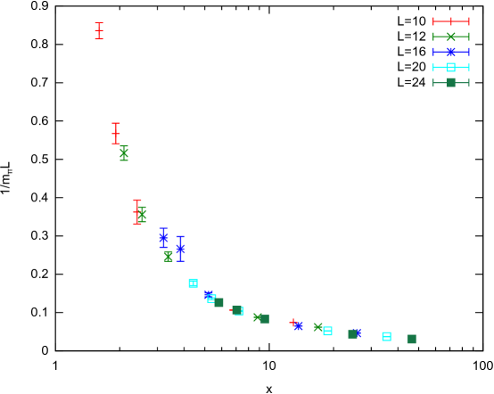
Figure 3: Collapse of $\pi$ data for $y_{m}=1.46$. Here and in the other figure, $x=mL^{y_{m}}$.

Using these results, and performing the minimization of (6.9) described above, we obtain values for $y_{m}$. In the case of $m_{a_{1}}$ and $f_{\pi}$, the quantity $\xi_{L}/L$ is small, and scaling violations [cf. Eq. (6.13)] can compete with the scaling function for small lattices. For this reason we exclude the small lattices $L/a=10,12$ for these channels. The results for $y_{m}$ are summarized in Table 2. It can be seen that each of the channels, and each of the fitting methods are consistent with each other within errors. The approximate collapse of data in the pion channel is shown in Fig. 3; the rho looks quite similar. In Fig. 4 we show the scatter that occurs for the $a_{1}$; for $f_{\pi}$ the spread in data is similar. In both cases it is the small $L$ observables that are pulling away from the curve. We interpret this as being due to scaling violations, though a thorough study extracting $\omega$ would be required to demonstrate this. Another interpretation is that the theory does not have an IRFP, and so the FSS fails for some channels. It is also possible that we are seeing the effect of $\beta=2.25$ not being close enough to the fixed point coupling (also scaling violations). We view the collapse seen in Fig. 3 as favoring our scaling violation interpretation.

Observable	Quadratic	Log Quad	PWL
$m_{\pi}$	1.67(93)	1.26(54)	1.51(33)
$m_{\rho}$	1.67(88)	1.37(39)	1.56(31)
$m_{a_{1}}$	1.40(52)	1.42(27)	1.41(22)
$f_{\pi}$	1.65(22)	1.49(54)	1.60(29)

Table 2: The scaling exponent $y_{m}=1+\gamma$ for the various observables and methods of interpolation. In parentheses, jackknife error is shown, obtained from eliminating one $m_{i,j}$ in all possible ways, in the minimization of (6.9). Because we use a large number of configurations, ${{\cal O}(10^{3})}$, statistical error is negligible by comparison. Weighted averages and standard deviations are shown in the last column.

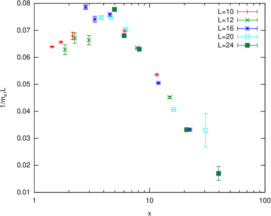
Figure 4: The $a_{1}$ data for $y_{m}=1.41$.

We average the twelve values of $y_{m}$ for the four channels and three fitting methods, weighted by the jackknife errors, to obtain $\overline{\gamma}=0.50$. The standard deviation of the twelve fits is 0.13. However, the smallest jackknife error from single elimination of data is 0.22. Treated as separate systematic errors, we obtain

$$\gamma=0.50\pm 0.26$$ (6.10)

In Table 3, we compare to other results using variety of methods. We are in agreement with all but the FSS studies [43, 44], though only 1.4$\sigma$ different from their upper limit.

Method	$\gamma$
SF [45]	$0.05<\gamma<0.56$
SF [46]	$0.31\pm 0.06$
Perturbative 4-loop [47]	$0.500$
Schwinger-Dyson [48]	$0.653$
All-orders hypothesis [49]	$0.46$
MCRG [50]	$-0.6<\gamma<0.6$
FSS [43]	$0.05<\gamma<0.20$
FSS [44]	$0.22\pm 0.06$
Mode number [51]	$0.371\pm 0.020$
FSS (here)	$0.50\pm 0.26$

Table 3: Summary of all MWTC results for the anomalous mass dimension. SF is Schrödinger functional and MCRG is Monte Carlo renormalization group. The perturbative result $\gamma=0.500$ was also given in the later, corrected version of [48], and relied on invariants calculated in [52].

6.3 Scaling of eigenvalues

In [38] DeGrand has fit the low-lying eigenvalues of the Dirac operator as a function of the lattice size $L$, based on theoretical developments in the older work [53]. The functional form is given by

$${\langle\lambda_{i}\rangle}\sim L^{-p},\quad p=\frac{d}{1+\alpha},\quad\alpha=\frac{d}{y_{m}}-1=\frac{3-\gamma}{1+\gamma}$$ (6.11)

where we remind the reader that in our conventions $y_{m}=1+\gamma$ and $d=4$. In DeGrand’s calculation he simulates tree-level clover improved sextet fermions and measures the eight lowest eigenvalues of the overlap Dirac operator on these configurations. As can be seen on the log-log plot of Fig. 8 of [38], a power law behavior is, broadly speaking, observed. Careful fitting is performed and it is found that the fit to a power law behavior is superior if only the four lowest eigenvalues are included. The answers for $\gamma$ have rather small error by this method, of order 3%. Concentrating on the three largest volumes and the four smallest eigenvalues, $p=1.59\pm 0.05$. After a bit of algebra using (6.11) above we find that $p=y_{m}$ and hence $\gamma=0.59\pm 0.05$, which is fairly consistent with what is found for the sextet model using other methods, such as the Schrödinger functional to be discussed below.

6.4 Other studies using finite size scaling

In [38] the FSS approach was found to yield $\gamma\approx 0.5$ for the SU(3) theory with $N_{f}=2$ sextet fermions. This is consistent with the Schrödinger functional results discussed in the next section. This paper also makes the important point that the value of $\gamma$ obtained should be independent of the bare coupling used in the simulation.

In [14], the authors use FSS to find $\gamma\sim 0.9$ for $N_{f}=1$ SU(2) adjoint. This large value of $\gamma$ is encouraging phenomenologically, and is similar to what was found for $N_{f}=10$ SU(3) fundamental [13]. It seems that theories that are right on the lower edge of the conformal window (and most likely below it) are the ones with $\gamma$ approaching 1.

The twelve flavor [SU(3) fundamental] theory has been studied using FSS by a few groups. In [39] DeGrand obtains $\gamma$ in five channels. He does not combine them to a final estimate, so we attempt to do that here. The unweighted average over the five channels is ${\bar{\gamma}}=0.33$. The r.m.s. average jackknife error is $0.24$. The standard deviation of the best fit values over the five channels is $0.07$. Combining these two sources of error in quadrature gives an overall error of $0.25$, for a final estimate $\gamma=0.33\pm 0.25$. FSS with scaling violations were considered in [26]; we will discuss this paper below in the section on scaling violations. The recent study [33] of the twelve flavor theory obtains highly consistent results with finite size scaling. They also include a correction to scaling with exponent $\omega$, which they estimate as $\omega\sim 0.23$; cf. their Fig. 13. All of the results for $\gamma$ have been summarized in Table 4.

Method	$\gamma$
FSS [39]	$0.33\pm 0.25$
Mode number [54]	$0.61\pm 0.05$
Hyperscaling [30]	0.4 to 0.5
Z factor [55]	0.044 ${}_{-0.024}^{+0.025}$ (stat.) ${}_{-0.032}^{+0.057}$ (syst.)
FSS w/ scale viol. [26]	0.235(15)
FSS w/ scale viol. [33]	0.235(46)
Z factor [56]	0.081 $\pm$ 0.018 (stat.) ${}_{-0}^{+0.025}$ (syst.)
Mode number [56]	$0.05\leq\gamma\leq 0.08$
4-loop [17, 18]	0.25

Table 4: Summary of twelve flavor estimates of the anomalous mass dimension. For the first entry, corresponding to [39], we have combined various results and errors as described in the text.

6.5 Forms of the scaling function

Here we consider the behavior of the function $f(x)$ appearing in (6.2), where $x=m^{1/y_{m}}L$ is the scaling variable. Asymptotically, it is natural to expect $f(x)\sim x^{\lambda}$; i.e., there is a leading power in the limit $x\to 0^{+}$. According to the analysis of [36] there are three basic cases that can occur. The first is that $f(x)$ is a pure power: $f(x)=Ax^{\lambda}$. This is unlikely to be the case in a theory with interactions. The second is the so-called simple case, $f(x)=x^{\lambda}f_{0}(x)$ where $f_{0}(x)=f_{0}+f_{1}x+f_{2}x^{2}+\cdots$, i.e., $f_{0}(x)$ is analytic about $x=0$. The third is the so-called complex case, $f(x)=x^{\lambda}f_{0}(x)$ where $f_{0}(x)$ is nonanalytic at $x=0$. In this third case, Fisher distinguishes two subcases. The first he calls “coincident weaker singularities,” where $|\ln f_{0}(x)|\to|\ln f_{0}|<\infty$ as $x\to 0$. As an example he gives $f_{0}(x)=f_{0}+f_{1}x^{\mu}+\cdots$ where $0<\mu<1$. The second he calls “divergent coincident singularities,” where $|\ln f_{0}(x)|\to\infty$ as $x\to 0$. As examples he gives $f_{0}(x)=(\ln x^{-1})^{\mu}f_{00}(x)$ or $f_{0}(x)=\exp[\nu(\ln x^{-1})^{\mu}]f_{00}$ [we have corrected what seems to be a typo in the second example].

So which type of behavior do we have in the gauge field theories that we are studying? Normally we think that it is necessary to take the thermodynamic limit $L\to\infty$ in order to develop thermodynamic singularities, and in particular for $\xi_{L}/L$ to become infinite. However, $x\to 0$ corresponds to holding $L$ finite while taking $m\to 0$. Fisher seems to imagine that this limit may yet lead to a singularity. In a quantum field theory there is an infinite number of degrees of freedom even at finite $L$, if we send the UV cutoff to infinity, i.e., $a\to 0$. Of course we have to renormalize and in a renormalizable theory this effectively replaces the contribution of the UV modes by finite quantities, so that it is as if we have a finite number of degrees of freedom when momentum is quantized due to finite $L$. We thus conclude that it is unlikely that we would realize the case of divergent coincident singularities. However, all of the other cases Fisher cites are open to us. In particular both the simple case and the coincident weaker singularities are distinct possibilities.

6.6 Corrections to scaling

6.6.1 Lattice spacing

The general scaling law for masses and decay constants is [after a slight redefinition of Eq. (6.2)]

$$\xi_{L}/L=f(mL^{y_{m}})$$ (6.12)

Often we simplify the notation to $x=mL^{y_{m}}$ and write $f(x)$. Corrections to scaling, or scaling violations, have additional terms, which at leading order take the form

$$\xi_{L}/L=f(mL^{y_{m}})+L^{-\omega}g(mL^{y_{m}})$$ (6.13)

[Alternatively, see (6.23) below.] Scaling violations have been incorporated into finite size scaling in the recent work [26]. This was used to resolve apparent discrepancies between the scaling exponent $\gamma$ according to different observables in the twelve fundamental flavor theory with gauge group $SU(3)$, which has been the source of much controversy.

Here we show that scaling violations and discretization errors may in some cases be the same thing. Corrections to scaling are not just a feature of continuum theories. Eq. (6.12) is written in lattice units. Restoring the lattice spacing, one has

$$\xi_{L}/L=f((ma)(L/a)^{y_{m}})$$ (6.14)

Now suppose there is discretization error that vanishes in the $a\to 0$ limit. Since we can only add dimensionless quantities to the above equation (the left-hand side is dimensionless), the discretization error can only enter through the combinations $ma$ and $a/L$. Thus the most general form of correction to scaling is $h(ma,a/L)$. Defining $x=(ma)(L/a)^{y_{m}}$ we see from

$$ma=(a/L)^{y_{m}}[(ma)(L/a)^{y_{m}}]$$ (6.15)

that $ma=(a/L)^{y_{m}}x$ and so we can redefine the scaling correction as

$$h(ma,a/L)\equiv{\tilde{h}}(a/L,x)$$ (6.16)

Expanding in $a$, holding $x$ fixed, we obtain

$${\tilde{h}}(a/L,x)=(a/L)^{\omega_{1}}g_{1}(x)+(a/L)^{\omega_{2}}g_{2}(x)+\cdots$$ (6.17)

where $\omega_{1}<\omega_{2}<\cdots$. Thus we see that (6.13) is the leading order correction in powers of the lattice spacing.

Irrelevant operators are also tied up with the scaling violations. By RG arguments given above, if $g_{i}$ are the irrelevant couplings and $y_{i}<0$ are their scaling dimensions, then

$$M_{H}/L=f(Lm^{1/y_{m}},g_{i}m^{-y_{i}/y_{m}})$$ (6.18)

In fact, the presence of irrelevant operators is often traced to the nonzero lattice spacing, so that there is a connection with the scaling violations that were discussed above. Next we specialize this to the gauge coupling, which is irrelevant in a theory with an IRFP.

6.6.2 Gauge coupling

Eq. (4.52) describes infinite volume. We can extend to $g\not=0$ (recall that $g\to g-g_{*}$ has been made) RG transformation,

$$C_{H}(t;{\hat{m}},g,L,\mu)=\lambda^{-2\gamma_{H}}C_{H}(t;{\hat{m}}^{\prime},g^{\prime},L,\mu^{\prime})$$ (6.19)

Repeating the steps in (4.4), we find that

$$C(t;{\hat{m}}^{\prime},g^{\prime},L,\mu^{\prime})=\lambda^{-2d_{H}}C(\lambda^{-1}t;{\hat{m}}^{\prime},g^{\prime},\lambda^{-1}L,\mu)$$ (6.20)

Again taking $\lambda^{-1}={\hat{m}}^{1/y_{m}}$, we find

$$C(t;{\hat{m}},g,L,\mu)=\mu^{2d_{H}}{\hat{m}}^{2\Delta_{H}/y_{m}}F(\mu{\hat{m}}^{1/y_{m}}t,1,{\hat{m}}^{-y_{g}/y_{m}}g,{\hat{m}}^{1/y_{m}}L\mu)$$ (6.21)

It follows that the “hadron” mass will satisfy

$$M_{H}L=f_{H}(x,{\hat{m}}^{-y_{g}/y_{m}}g),\quad x={\hat{m}}^{1/y_{m}}L$$ (6.22)

In [26] this is expanded about small $g$ to obtain

$$M_{H}L=F_{H}(x)\left(1+G_{H}(x){\hat{m}}^{-y_{g}/y_{m}}g+{{\cal O}(g^{2})}\right)$$ (6.23)

They furthermore approximate $G_{H}(x)$ as a constant $c_{G}$ over the range of $x$ that they consider. Defining $\omega=-y_{g}/y_{m}$ and $c_{0}=c_{G}g$, they fit the spectrum to

$$\frac{M_{H}L}{1+c_{0}m^{\omega}}=F_{H}(x)$$ (6.24)

allowing $c_{0}$ and $\omega$ to be optimized in the fit, and $F_{H}(x)$ as the concatenation of two quadratic functions whose coefficients are also fit. Finally, the $c_{0}$ values are allowed to be different for each value of the bare lattice coupling $\beta_{F}$ that multiplies the part of the gauge action in the fundamental representation. (Their simulation also involve an adjoint gauge action with coefficient $\beta_{A}$.) They are able to obtain reasonably consistent values for the exponents when the pion, rho and pion decay constant are included in a combined fit, although the $\chi^{2}$ increases by a factor of two compared to the fit with only the pion mass.

7 Schrödinger functional

The Schrödinger functional approach simulates on the four-dimensional cylinder $W\times{\bf T}^{3}$ where $W=[0,T]$ is a section of the real line and ${\bf T}^{3}$ is a three-torus. The three torus is represented as a cubic lattice with $L/a$ sites in each direction, and periodic boundary conditions. The temporal extent is related to the spatial extent by a fixed aspect ratio, $T=\zeta L$. The boundary conditions at the boundaries $t=0$ and $t=T$ are such that the classical solution to the field equations corresponds to a constant ${{\cal O}(1/L)}$ chromoelectric field. A classic use of this is to obtain the running coupling by measuring the response of the system to this background chromoelectric field. However, it can also be used for determining the renormalization constant associated with the mass operator ${\bar{\psi}}\psi$, and hence the anomalous mass dimension. Recently it has also been discussed in the context of determining the anomalous dimension of four-fermion operators, which may play an important role in modifying the predictions of walking technicolor theories.

7.1 Anomalous mass dimension

The renormalization of the quark mass and the corresponding anomalous dimension in the Schrödinger functional scheme was developed originally in [57, 58, 59]. Its early use in the context of walking technicolor was seen in [45].

The method here begins with the partially conserved axial current (PCAC) relation. This can be written

$$Z_{A}{\partial}_{\mu}A_{\mu}^{a}=2m_{\text{ren.}}Z_{P}P^{a}$$ (7.1)

where $A_{\mu}^{a}$ and $P^{a}$ are the bare axial current and pseudoscalar density. $Z_{A}$ and $Z_{P}$ are renormalization constants, and $m_{\text{ren.}}$ is the renormalized PCAC mass (we assume a degenerate $N_{f}$ flavor model). On the other hand we have the bare relation

$${\partial}_{\mu}A_{\mu}^{a}=2m_{\text{latt.}}P^{a}$$ (7.2)

Comparing these two we see that

$$m_{\text{latt.}}=m_{\text{ren.}}\frac{Z_{P}}{Z_{A}}$$ (7.3)

The quantity $m_{\text{latt.}}$ is obtained from lattice correlation functions without any reference to the renormalization scale $\mu$, hence is $\mu$ independent. From this we immediately obtain

$$\gamma_{m}=-\frac{d\ln m_{\text{ren.}}}{d\ln\mu}=\frac{d}{d\ln\mu}\ln\left(\frac{Z_{P}}{Z_{A}}\right)$$ (7.4)

The renormalization factor $Z_{A}$ is conventionally determined by the requirement that the current algebra take its canonical form. As a result of the nonlinearity of this set of relations, the anomalous dimension of $Z_{A}$ must vanish,

$$\frac{d\ln Z_{A}}{d\ln\mu}=0$$ (7.5)

The result is therefore that

$$\gamma_{m}=\frac{d\ln Z_{P}}{d\ln\mu}$$ (7.6)

That is, the anomalous mass dimension can be determined from the pseudoscalar density renormalization factor. It is interesting that this density is related to the scalar density ${\bar{\psi}}\psi$, normally associated with $\gamma_{m}$, by a chiral rotation.

In the Schrödinger functional approach, $\mu=1/L$. Hence

$$\gamma_{m}=-\frac{d\ln Z_{P}}{d\ln L}$$ (7.7)

We must now explain how $Z_{P}$ is obtained. One introduces a notation for the boundary fermions

$$\zeta({\bf x})=q(0,{\bf x}),\quad\zeta^{\prime}({\bf x})=q(T-1,{\bf x}),$$

$${\bar{\zeta}}({\bf x})={\bar{q}}(0,{\bf x}),\quad{\bar{\zeta}}^{\prime}({\bf x})={\bar{q}}(T-1,{\bf x})$$ (7.8)

Adopting the notation of [57], one then forms correlation functions involving the boundary fields:

$$f_{P}(x_{0}) = -\frac{1}{3}\sum_{{\bf y},{\bf z}}\langle P^{a}(x){\bar{\zeta}}({\bf y})\gamma_{5}\frac{1}{2}\tau^{a}\zeta({\bf z})\rangle$$

$$f_{1} = -\frac{1}{3L^{6}}\sum_{{\bf u},{\bf v},{\bf y},{\bf z}}\langle{\bar{\zeta}}^{\prime}({\bf u})\gamma_{5}\frac{1}{2}\tau^{a}\zeta^{\prime}({\bf v}){\bar{\zeta}}({\bf y})\gamma_{5}\frac{1}{2}\tau^{a}\zeta({\bf z})\rangle$$ (7.9)

The renormalized versions of these are

$$f_{P}^{\text{ren.}}=Z_{P}Z_{\zeta}^{-1}f_{P},\quad f_{1}^{\text{ren.}}=Z_{\zeta}^{-2}f_{1}$$ (7.10)

where $Z_{\zeta}$ is the wavefunction renormalization of the $\zeta,\zeta^{\prime}$ boundary fields, e.g., $\zeta=\sqrt{Z_{\zeta}}\zeta_{\text{ren.}}$. Then it is easy to see that

$$Z_{P}=\frac{f_{P}^{\text{ren.}}(x_{0})}{\sqrt{f_{1}^{\text{ren.}}}}\frac{\sqrt{f_{1}}}{f_{P}(x_{0})}$$ (7.11)

One typically chooses $x_{0}=T/2$. To a certain extent, the renormalized values $f_{P}^{\text{ren.}}(T/2)$ and $f_{1}^{\text{ren.}}$ are arbitrary, so the convention is to take these equal to the tree-level values

$$\frac{f_{P}^{\text{ren.}}(T/2)}{\sqrt{f_{1}^{\text{ren.}}}}\equiv\frac{f_{P}^{\text{tree}}(T/2)}{\sqrt{f_{1}^{\text{tree}}}}\equiv c$$ (7.12)

Then

$$Z_{P}=c\frac{\sqrt{f_{1}}}{f_{P}(T/2)}$$ (7.13)

The constant $c$ evaluates to

$$c=\sqrt{N_{c}}+{{\cal O}(a^{2})}$$ (7.14)

so that it is $L$ independent. Thus we arrive at a somewhat strange situation where the renormalized ratio in (7.12) is independent of the RG scale $\mu=1/L$ whereas the bare ratio $\sqrt{f_{1}}/f_{P}(T/2)$ carries all of the $\mu=1/L$ dependence. This is a consequence of choosing the scheme (7.12) and identifying $\mu$ with the inverse size of the lattice $1/L$.

It is interesting to contrast this with what would happen with periodic boundary conditions with $t$ now ranging $t=0,a,2a,\ldots,2L-a$. One could retain the “boundary” fields (7.8) but with $T\to L$, which are really just fields on the timeslice at the origin, and the midpoint timeslice. However now the correlation function (7.9) have the dependence on $L$ of (they involve pseudoscalar operators, and are hence dominated by the pion):

$$f_{P}(x_{0})\sim e^{-m_{\pi}x_{0}}+e^{-m_{\pi}(2L-x_{0})},\quad\sqrt{f_{1}}\sim e^{-m_{\pi}L/2}$$ (7.15)

Forming the relevant ratio

$$\frac{f_{P}(x_{0})}{\sqrt{f_{1}}}\sim e^{-m_{\pi}(x_{0}-L/2)}+e^{-m_{\pi}(3L/2-x_{0})}$$ (7.16)

we see that there is no choice of $x_{0}$ which would cancel the $L$ dependence. The result is that the constant $c$ which would appear in

$$Z_{P}=c\frac{\sqrt{f_{1}}}{f_{P}(x_{0})}$$ (7.17)

would not be independent of $L$, and it would need to be known in order to obtain the anomalous mass dimension. This shows the clear superiority of the Schrödinger functional approach.

As an example of this method, in [60] the anomalous mass dimension was obtained for sextet “QCD.” Because of a slow running that was observed, they were able to fit to

$$Z_{P}(L)=Z_{P}(L_{0})\left(\frac{L_{0}}{L}\right)^{\gamma}$$ (7.18)

to obtain $\gamma$. One sees from their analysis that $\gamma\mathrel{\hbox to0.0pt{\raise 2.15277pt\hbox{$<$}\hss}{\lower 2.15277pt\hbox{$\sim$}}}0.4$ for the action that is able to probe the strong coupling regime where the fixed point is supposed to exist. This approach has also been used for SU(2) with two flavors in the adjoint representation [45, 46]. The results have been presented above in Table 3. Another study of the anomalous mass dimension using the Schrödinger functional technique is [61]. There they study SU(2) gauge theory with six flavors of fundamental representation fermions. They obtain $0.26\mathrel{\hbox to0.0pt{\raise 2.15277pt\hbox{$<$}\hss}{\lower 2.15277pt\hbox{$\sim$}}}\gamma\mathrel{\hbox to0.0pt{\raise 2.15277pt\hbox{$<$}\hss}{\lower 2.15277pt\hbox{$\sim$}}}0.74$. In [62], SU(4) gauge theory with decuplet fermions was studied, yielding $\gamma\sim 0.4$, quite similar to what was seen for SU(2) and SU(3) two-index symmetric representation fermions.

7.2 Four-fermion operators

Ref. [63] takes some preliminary steps toward using the Schrödinger functional to determine the anomalous dimensions of four-fermion operators. This is a very important direction to explore, because one would like to obtain the full spectrum of critical indices in an interacting four-dimensional conformal field theory. An alternative method would be to include the four-fermion operator in the lattice action, and then use finite size scaling with the coefficient of that operator.

8 The eigenmode number approach

8.1 Early steps

In [64] it was shown that the scaling (4.7) implies that the density of Dirac eigenvalues $\rho(\lambda)$ has the behavior

$$\rho(\lambda)\sim\lambda^{\eta_{{\bar{\psi}}\psi}}$$ (8.1)

This was rederived in [22]. Hence we can measure the spectrum of $D$ and obtain an estimate of $\gamma_{*}$.

8.2 The mode number development

Related to the eigenvalue distribution $\rho(\lambda)$, one can define a quantity known as the “mode number” which has a number of useful properties. In [51] a precise result was achieved, $\gamma_{m}=0.371(20)$ for SU(2) with two Dirac flavors in the adjoint representation. Other recent results using this method include [54, 65, 66, 67, 68, 69, 28, 70, 71, 72]. For instance in [54] it was found in the SU(3) twelve flavor theory that $\gamma=0.61(5)$. The integral of the spectral density $\rho(\lambda)$ of the Dirac operator (a.k.a. the mode number $\nu(\lambda_{\text{max}})$) is used to predict the anomalous dimension of the mass operator. On the lattice with Wilson type fermions the spectrum is complex, so what one actually looks at is

$$D_{L}^{\dagger}D_{L}\psi_{\lambda}=|\lambda|^{2}\psi_{\lambda}$$ (8.2)

so that it is really $\rho(|\lambda|)$ which is analyzed. Some analyses also use eigenvalues $\mu^{2}$ of the massive operator $D_{L}^{\dagger}D_{L}+m^{2}$, in which case eigenvalues are obtained as $|\lambda|^{2}=\mu^{2}-m^{2}$. For small values of $|\lambda|$ the eigenvalues are almost imaginary, so this becomes equivalent to the Euclidean continuum spectral density

$$D_{C}\psi_{\lambda}=i\lambda\psi_{\lambda}$$ (8.3)

$\rho=\rho(\lambda)$ up to lattice artifacts and an obvious double-counting related to the fact that for every nonzero eigenvalue $i\lambda$ there is a corresponding eigenvalue $i\lambda^{\prime}=-i\lambda$. From this point on we will simply write $\lambda$ rather than $|\lambda|$, ignoring this lattice detail.

From RG arguments, reviewed above, we know that

$$\rho(\lambda)\sim\lambda^{(3-\gamma)/(1+\gamma)}$$ (8.4)

The mode number is then determined from

$$\nu(\lambda_{\text{max}})=V\int_{0}^{\lambda_{\text{max}}}d\lambda~{}\rho(\lambda)$$ (8.5)

where $V$ is the volume of space. If the massive Dirac operator is used, then the mode number also depends on this quantity: $\nu=\nu(\lambda_{\text{max}},m)$. The chiral condensate, in the case of spontaneous chiral symmetry breaking, can be obtained from the mode number according to the formula [73]

$$\Sigma=\frac{\pi}{2V}\frac{d\nu}{d\lambda_{\text{max}}}$$ (8.6)

One of the advantages to using the mode number is that it is known to be renormalization group invariant [74, 73]. In addition, the eigenvalues are only multiplicatively renormalized. Hence, we avoid the divergent (${{\cal O}(1/a^{3})}$ at finite lattice spacing) subtractions that would be necessary if we were to use the condensate relation (4.7). Note that the multiplicative renormalization is a non-issue because if $\lambda=Z\lambda_{0}$ relates the renormalized and bare eigenvalue, we still have

$$\rho(\lambda_{0})\sim\lambda_{0}^{(3-\gamma)/(1+\gamma)}$$ (8.7)

All that has happened is that the constant of proportionality has been modified. Another advantage of the mode number method that should be emphasized is that it allows the determination of $\gamma$ from a single lattice simulation. By contrast, the finite size scaling approach requires many $L,m$ values to be simulated (although many of these can be small $L$ and larger $m$, so the actual computational cost is not that high). However, the most significant benefit seems to be accuracy.

In practice, a finite mass should be simulated in order to avoid large finite volume effects. In addition, the anomalous dimension that we are interested in is a property of the IR of the theory. Thus one must find an optimal window $\lambda_{1}<\lambda<\lambda_{2}$ where the fit should be applied. How does one determine this window? $\lambda_{2}$ can be identified because of asymptotic freedom: at large $\lambda$ the anomalous dimension vanishes and $\rho\sim\lambda^{3}$. So one avoids that region by taking $\lambda_{2}$ sufficiently small. $\lambda_{1}$ can be identified from the fact that it is mass-dependent. Looking at the scaling of $\rho$ at small $\lambda$, one looks for the region that changes its behavior significantly as the mass is adjusted. Clearly there is some uncertainty in choosing the optimum values of $\lambda_{1,2}$, but this is no different than any other method—we characterize this a systematic uncertainty. The encouraging fact found in [51] is that the PCAC mass does not need to be very small in order to open up a reasonable window and obtain accurate results for $\gamma$. Indeed other groups have also applied this method with much success.

One powerful technique can be applied here which is a stochastic determination of the mode number

$$\nu(\Omega)=\frac{1}{V}{\langle\mathop{{\hbox{Tr}\,}}\nolimits\mathbb{P}\rangle}$$ (8.8)

where $\mathbb{P}$ is a projector

$$\mathbb{P}=h^{4}\left(1-\frac{2\Omega_{*}^{2}}{D^{\dagger}D+\Omega_{*}^{2}}\right)$$ (8.9)

where $h(x)$ is a polynomial that approximates $\theta(-x)$ within a particular range of $|x|$. The traces of inverses are computed by solving (e.g., using conjugate gradient)

$$(D^{\dagger}D+\Omega_{*}^{2})^{n}(x,y)X_{i}(y)=\eta_{i}(x)$$ (8.10)

with $N_{r}$ random sources $\eta_{i}$. Then

$$\mathop{{\hbox{Tr}\,}}\nolimits(D^{\dagger}D+\Omega_{*}^{2})^{-n}=\frac{1}{N_{r}V}\sum_{i,x}\mathop{{\hbox{Tr}\,}}\nolimits_{s.c.}(X_{i}(x)\eta_{i}^{*}(x))+{{\cal O}(1/\sqrt{N_{r}})}$$ (8.11)

where the trace on the r.h.s. is only over spin and color indices. Typically one fully dilutes over spin-color indices (factor of 12) and $N_{r}={{\cal O}(10^{2})}-{{\cal O}(10^{3})}$ may be required for an accurate estimate. These inversions must be performed on each gauge field configuration. This is a perfect workload for GPUs, which optimally perform a large number of inversions. It would also entail a small project to modify the GPU code (probably QUDA) to implement $(D^{\dagger}D+\Omega_{*}^{2})^{n}$ inside the inverter. Note also that we only need to perform the inversions for the largest power of $n$ appearing in $h^{4}(x)$, since traces of lower powers can be obtained from

$$\mathop{{\hbox{Tr}\,}}\nolimits(D^{\dagger}D+\Omega_{*}^{2})^{-(n-m)}=\frac{1}{N_{r}V}\sum_{i,x,y}\mathop{{\hbox{Tr}\,}}\nolimits_{s.c.}((D^{\dagger}D+\Omega_{*}^{2})^{m}(x,y)X_{i}(y)\eta_{i}^{*}(x))$$ (8.12)

The lattice data is fit to

$$a^{-4}\nu(\Omega)=a^{-4}\nu_{0}+A[(a\Omega)^{2}-(am)^{2}]^{2/(1+\gamma)}$$ (8.13)

Here, $m=Z_{A}m_{\text{PCAC}}$ where $m_{\text{PCAC}}$ is the bare PCAC mass. It is amusing that since $m_{\text{PCAC}}$ is known and $m$ is obtained from the fit, the mode number analysis provides a way to obtain the renormalization constant $Z_{A}$.

The mode number analysis has been extended to address a scale dependent anomalous mass dimension $\gamma(\mu)$ in [67]. This is a method that can be applied both in theories with a conformal fixed point, and in theories that are confining in the infrared. In [67] it is shown how to combine lattices of different volumes and bare couplings in order to obtain a more complete picture. This provides added confidence in the approach because they are able to follow the dynamics from asymptotic freedom in the ultraviolet to spontaneous chiral symmetry breaking in the infrared in the context of the $N_{f}=4$ theory (SU(3) with fundamental flavors).

In this study, the matching of different $\beta$ was done with the following rescaling of the eigenvalues $\lambda$ for $\gamma<2$:

$$\lambda^{\prime}=\left(\frac{a}{a^{\prime}}\right)^{1+\gamma}\lambda$$ (8.14)

This is based on the fact that the eigenvalues should scale like the mass parameter. For the infrared where couplings are larger and $\gamma>2$, the prescription in [67] is to terminate the above scaling at $\gamma=2$ and replace it with

$$\lambda^{\prime}=\left(\frac{a}{a^{\prime}}\right)^{2}\lambda$$ (8.15)

for $\gamma>2$. Empirically, this causes the curves to fall on top of each other giving a fairly smooth overall curve.

Recently, in an effort to better understand the systematic uncertainties associated with the mode number approach, Keegan has studied the Schwinger model, where analytic results are also available [72]. This paper considers the $N_{f}=0,2$ models with small fermion mass and follows an approach similar to [67] in that it connects a range of $\beta$ values by rescaling the eigenvalues by a power of the lattice spacing. By doing this, Keegan is able to go from very small eigenvalues to very large eigenvalues and follow the flow of $\gamma(\lambda)$. Indeed, in the $N_{f}=2$ model he sees that in the IR $\gamma\approx 0.5$, consistent with the analytic prediction, and that in the UV $\gamma\approx 0$, also consistent with the analytic prediction (asymptotic freedom). In addition he uses the spectral density $\rho(\lambda)$ directly and finds a consistent result, though with much larger statistical errors. This work clears up the contradiction found in [69], which only used one value of $\beta$.

Ref. [14] uses the mode number to find $\gamma\sim 0.9$ for $N_{f}=1$ SU(2) adjoint, consistent with what they found using finite size scaling. This rather large value is another indication that theories at the lower edge of the conformal window are the ones that are the most likely to be phenomenologically viable in terms of the size of $\gamma$. Another interesting development is the recent paper [71], which used Eguchi-Kawai reduction with the mode number to estimate $\gamma$ in the large $N_{c}$ limit.

9 Conclusions

Because of its phenomenological importance, the anomalous mass dimension in conformal and nearly conformal theories is the quantity that has been most studied on the lattice in the last few years. As has been seen in this review, a number of techniques have been developed for obtaining fairly accurate estimates. Additional exponents, such as the correction to scaling index, are beginning to also be included. It is hoped that the coming years will see the computation of other critical exponents in conformal field theories on the lattice.

We have learned various facts about the anomalous mass dimension of phenomenological importance. It seems that it is the theories that are on the lower edge of the conformal window which have $\gamma\approx 1$, and in other conformal theories $\gamma$ is too small. Four fermion operators coming from extended technicolor have been suggested as a way to push theories out of the conformal window and increase $\gamma$, as is needed for a viable walking technicolor theory [11]. Alternatively, giving mass to some subset of the fermions may also produce the same effect [75]. In both cases it would be very useful to have careful studies of the anomalous mass dimension from the lattice.

References

- [1] K. G. Wilson, Operator product expansions and anomalous dimensions in the thirring model, Phys. Rev. D2 (1970) 1473.
- [2] K. G. Wilson, Anomalous dimensions and the breakdown of scale invariance in perturbation theory, Phys.Rev. D2 (1970) 1478.
- [3] A. Patashinskii and V. Pokrovskii, Behavior of ordered systems near the transition point, Sov. Phys. JETP 23 (1966) 292.
- [4] T. Banks and A. Zaks, On the Phase Structure of Vector-Like Gauge Theories with Massless Fermions, Nucl.Phys. B196 (1982) 189.
- [5] R. S. Chivukula and E. H. Simmons, Condensate Enhancement and D-Meson Mixing in Technicolor Theories, Phys. Rev. D82 (2010) 033014, [1005.5727].
- [6] J. Kuti, The Higgs particle and the lattice, PoS LATTICE2013 (2014) 004.
- [7] L. Del Debbio, IR fixed points in lattice field theories, Int. J. Mod. Phys. A29 (2014) 1445006.
- [8] T. DeGrand, Lattice tests of beyond Standard Model dynamics, 1510.05018.
- [9] M. P. Lombardo, K. Miura, T. J. Nunes da Silva and E. Pallante, One, two, zero: Scales of strong interactions, Int. J. Mod. Phys. A29 (2014) 1445007, [1410.2036].
- [10] R. Foadi, M. T. Frandsen and F. Sannino, 125 GeV Higgs from a not so light Technicolor Scalar, Phys.Rev. D87 (2013) 095001, [1211.1083].
- [11] H. S. Fukano and F. Sannino, Conformal Window of Gauge Theories with Four-Fermion Interactions and Ideal Walking, Phys.Rev. D82 (2010) 035021, [1005.3340].
- [12] J. Erdmenger, N. Evans and M. Scott, Meson spectra of asymptotically free gauge theories from holography, Phys. Rev. D91 (2015) 085004, [1412.3165].
- [13] T. Appelquist et al., Approaching Conformality with Ten Flavors, 1204.6000.
- [14] A. Athenodorou, E. Bennett, G. Bergner and B. Lucini, Infrared regime of SU(2) with one adjoint Dirac flavor, Phys. Rev. D91 (2015) 114508, [1412.5994].
- [15] M. Testa, Some observations on broken symmetries, JHEP 9804 (1998) 002, [hep-th/9803147].
- [16] DESY-Munster-Roma Collaboration collaboration, F. Farchioni et al., The Supersymmetric Ward identities on the lattice, Eur.Phys.J. C23 (2002) 719–734, [hep-lat/0111008].
- [17] K. G. Chetyrkin, Quark mass anomalous dimension to O(), Phys. Lett. B404 (1997) 161–165, [hep-ph/9703278].
- [18] J. A. M. Vermaseren, S. A. Larin and T. van Ritbergen, The four loop quark mass anomalous dimension and the invariant quark mass, Phys. Lett. B405 (1997) 327–333, [hep-ph/9703284].
- [19] G. Mack, All Unitary Ray Representations of the Conformal Group SU(2,2) with Positive Energy, Commun.Math.Phys. 55 (1977) 1.
- [20] S. Minwalla, Restrictions imposed by superconformal invariance on quantum field theories, Adv.Theor.Math.Phys. 2 (1998) 781–846, [hep-th/9712074].
- [21] K. Wiegandt, Perturbative Methods for Superconformal Quantum Field Theories in String - Gauge Theory Dualities, 1212.5181.
- [22] L. Del Debbio and R. Zwicky, Hyperscaling relations in mass-deformed conformal gauge theories, Phys.Rev. D82 (2010) 014502, [1005.2371].
- [23] LatKMI collaboration, Y. Aoki et al., Composite flavor-singlet scalar in twelve-flavor QCD, PoS LATTICE2013 (2014) 077, [1311.6885].
- [24] M. Luscher, Properties and uses of the Wilson flow in lattice QCD, JHEP 1008 (2010) 071, [1006.4518].
- [25] M. E. Fisher, Renormalization group theory, the epsilon expansion, and Ken Wilson as I knew him, in Ken Wilson Memorial Volume: Renormalization, Lattice Gauge Theory, the Operator Product Expansion and Quantum Fields (B. E. Baaquie, K. Huang, M. E. Peskin and K. K. Phua, eds.), (Singapore), World Scientific, 2015.
- [26] A. Cheng, A. Hasenfratz, Y. Liu, G. Petropoulos and D. Schaich, Finite size scaling of conformal theories in the presence of a near-marginal operator, Phys. Rev. D90 (2014) 014509, [1401.0195].
- [27] J. L. Cardy, Scaling and renormalization in statistical physics. Cambridge University Press, Cambridge, United Kingdom, 1996.
- [28] L. Del Debbio, B. Lucini, C. Pica, A. Patella, A. Rago and S. Roman, Large-volume results in SU(2) with adjoint fermions, in Proceedings, 31st International Symposium on Lattice Field Theory (Lattice 2013), 2013. 1311.5597.
- [29] Z. Fodor, K. Holland, J. Kuti, D. Nogradi, C. Schroeder et al., Twelve massless flavors and three colors below the conformal window, Phys.Lett. B703 (2011) 348–358, [1104.3124].
- [30] Y. Aoki, T. Aoyama, M. Kurachi, T. Maskawa, K.-i. Nagai, H. Ohki et al., Lattice study of conformality in twelve-flavor QCD, Phys. Rev. D86 (2012) 054506, [1207.3060].
- [31] LatKMI collaboration, Y. Aoki et al., Light composite scalar in eight-flavor QCD on the lattice, Phys. Rev. D89 (2014) 111502, [1403.5000].
- [32] LatKMI collaboration, Y. Aoki et al., Conformality in twelve-flavor QCD, PoS LATTICE2014 (2015) 256, [1501.06660].
- [33] M. P. Lombardo, K. Miura, T. J. N. da Silva and E. Pallante, On the particle spectrum and the conformal window, JHEP 12 (2014) 183, [1410.0298].
- [34] M. Stephanov, Deconstruction of Unparticles, Phys.Rev. D76 (2007) 035008, [0705.3049].
- [35] M. E. Peskin and D. V. Schroeder, An introduction to quantum field theory. Addison-Wesley, Reading, Massachusetts, 1995.
- [36] M. E. Fisher, The theory of critical point singularities, in Critical phenomena, Proceedings of the 51st Enrico Fermi Summer School, Varenna (M. S. Green, ed.), (New York), Academic Press, 1971.
- [37] M. E. Fisher and M. N. Barber, Scaling Theory for Finite-Size Effects in the Critical Region, Phys.Rev.Lett. 28 (1972) 1516–1519.
- [38] T. DeGrand, Finite-size scaling tests for SU(3) lattice gauge theory with color sextet fermions, Phys.Rev. D80 (2009) 114507, [0910.3072].
- [39] T. DeGrand, Finite-size scaling tests for spectra in SU(3) lattice gauge theory coupled to 12 fundamental flavor fermions, Phys.Rev. D84 (2011) 116901, [1109.1237].
- [40] J. Giedt and E. Weinberg, Finite size scaling in minimal walking technicolor, Phys.Rev. D85 (2012) 097503, [1201.6262].
- [41] S. M. Bhattacharjee and F. Seno, A measure of data collapse for scaling, Jour. of Phys. A34 (2001) 6375.
- [42] J. Giedt and E. Weinberg, Backward running or absence of running from Creutz ratios, Phys.Rev. D84 (2011) 074501, [1105.0607].
- [43] L. Del Debbio, B. Lucini, A. Patella, C. Pica and A. Rago, Mesonic spectroscopy of Minimal Walking Technicolor, Phys.Rev. D82 (2010) 014509, [1004.3197].
- [44] L. Del Debbio, B. Lucini, A. Patella, C. Pica and A. Rago, The infrared dynamics of Minimal Walking Technicolor, Phys.Rev. D82 (2010) 014510, [1004.3206].
- [45] F. Bursa, L. Del Debbio, L. Keegan, C. Pica and T. Pickup, Mass anomalous dimension in SU(2) with two adjoint fermions, Phys.Rev. D81 (2010) 014505, [0910.4535].
- [46] T. DeGrand, Y. Shamir and B. Svetitsky, Infrared fixed point in SU(2) gauge theory with adjoint fermions, Phys. Rev. D83 (2011) 074507, [1102.2843].
- [47] C. Pica and F. Sannino, UV and IR Zeros of Gauge Theories at The Four Loop Order and Beyond, Phys.Rev. D83 (2011) 035013, [1011.5917].
- [48] T. A. Ryttov and R. Shrock, Higher-Loop Corrections to the Infrared Evolution of a Gauge Theory with Fermions, Phys.Rev. D83 (2011) 056011, [1011.4542].
- [49] C. Pica and F. Sannino, Beta Function and Anomalous Dimensions, Phys.Rev. D83 (2011) 116001, [1011.3832].
- [50] S. Catterall, L. Del Debbio, J. Giedt and L. Keegan, MCRG Minimal Walking Technicolor, Phys. Rev. D85 (2012) 094501, [1108.3794].
- [51] A. Patella, A precise determination of the psibar-psi anomalous dimension in conformal gauge theories, Phys.Rev. D86 (2012) 025006, [1204.4432].
- [52] M. Mojaza, C. Pica and F. Sannino, Hot Conformal Gauge Theories, Phys.Rev. D82 (2010) 116009, [1010.4798].
- [53] G. Akemann, P. H. Damgaard, U. Magnea and S. M. Nishigaki, Multicritical microscopic spectral correlators of Hermitian and complex matrices, Nucl. Phys. B519 (1998) 682–714, [hep-th/9712006].
- [54] A. Cheng, A. Hasenfratz and D. Schaich, Novel phase in SU(3) lattice gauge theory with 12 light fermions, Phys. Rev. D85 (2012) 094509, [1111.2317].
- [55] E. Itou, A novel scheme for the wave function renormalization of the composite operators, PTEP 2015 (2015) 043B08, [1307.6645].
- [56] E. Itou and A. Tomiya, Determination of the mass anomalous dimension for and SU() gauge theories, 1411.1155.
- [57] ALPHA collaboration, S. Sint and P. Weisz, The Running quark mass in the SF scheme and its two loop anomalous dimension, Nucl. Phys. B545 (1999) 529–542, [hep-lat/9808013].
- [58] ALPHA collaboration, S. Capitani, M. Luscher, R. Sommer and H. Wittig, Nonperturbative quark mass renormalization in quenched lattice QCD, Nucl. Phys. B544 (1999) 669–698, [hep-lat/9810063].
- [59] ALPHA collaboration, M. Della Morte, R. Hoffmann, F. Knechtli, J. Rolf, R. Sommer, I. Wetzorke et al., Non-perturbative quark mass renormalization in two-flavor QCD, Nucl. Phys. B729 (2005) 117–134, [hep-lat/0507035].
- [60] T. DeGrand, Y. Shamir and B. Svetitsky, Mass anomalous dimension in sextet QCD, Phys. Rev. D87 (2013) 074507, [1201.0935].
- [61] M. Hayakawa, K. I. Ishikawa, S. Takeda and N. Yamada, Running coupling constant and mass anomalous dimension of six-flavor SU(2) gauge theory, Phys. Rev. D88 (2013) 094504, [1307.6997].
- [62] T. DeGrand, Y. Shamir and B. Svetitsky, SU(4) lattice gauge theory with decuplet fermions: Schrodinger functional analysis, Phys. Rev. D85 (2012) 074506, [1202.2675].
- [63] L. Del Debbio, L. Keegan and C. P. Ruano, Four-fermi anomalous dimension with adjoint fermions, PoS LATTICE2014 (2014) 260.
- [64] T. DeGrand, Volume scaling of Dirac eigenvalues in SU(3) lattice gauge theory with color sextet fermions, 0906.4543.
- [65] A. Hasenfratz, A. Cheng, G. Petropoulos and D. Schaich, Mass anomalous dimension from Dirac eigenmode scaling in conformal and confining systems, PoS LATTICE2012 (2012) 034, [1207.7162].
- [66] P. de Forcrand, S. Kim and W. Unger, Conformality in many-flavour lattice QCD at strong coupling, JHEP 02 (2013) 051, [1208.2148].
- [67] A. Cheng, A. Hasenfratz, G. Petropoulos and D. Schaich, Scale-dependent mass anomalous dimension from Dirac eigenmodes, JHEP 1307 (2013) 061, [1301.1355].
- [68] A. Cheng, A. Hasenfratz, G. Petropoulos and D. Schaich, Determining the mass anomalous dimension through the eigenmodes of Dirac operator, PoS LATTICE2013 (2014) 088, [1311.1287].
- [69] D. Landa-Marban, W. Bietenholz and I. Hip, Features of a 2d Gauge Theory with Vanishing Chiral Condensate, Int. J. Mod. Phys. C25 (2014) 1450051, [1307.0231].
- [70] K. Cichy, Quark mass anomalous dimension and from the twisted mass Dirac operator spectrum, JHEP 08 (2014) 127, [1311.3572].
- [71] M. García Pérez, A. González-Arroyo, L. Keegan and M. Okawa, Mass anomalous dimension of Adjoint QCD at large N from twisted volume reduction, JHEP 08 (2015) 034, [1506.06536].
- [72] L. Keegan, Schwinger Model Mass Anomalous Dimension, in 33rd International Symposium on Lattice Field Theory (Lattice 2015) Kobe, Japan, July 14-18, 2015, 2015. 1508.01685.
- [73] L. Giusti and M. Luscher, Chiral symmetry breaking and the Banks-Casher relation in lattice QCD with Wilson quarks, JHEP 0903 (2009) 013, [0812.3638].
- [74] L. Del Debbio, L. Giusti, M. Luscher, R. Petronzio and N. Tantalo, Stability of lattice QCD simulations and the thermodynamic limit, JHEP 02 (2006) 011, [hep-lat/0512021].
- [75] R. Brower, A. Hasenfratz, C. Rebbi, E. Weinberg and O. Witzel, Targeting the conformal window with 4+8 flavors, PoS LATTICE2014 (2014) 254, [1411.3243].