Exciton band structure in two-dimensional materials

Abstract

Low-dimensional materials differ from their bulk counterpart in many respects. In particular, the screening of the Coulomb interaction is strongly reduced, which can have important consequences such as the significant increase of exciton binding energies. In bulk materials the binding energy is used as an indicator in optical spectra to distinguish different kinds of excitons, but this is not possible in low-dimensional materials, where the binding energy is large and comparable in size for excitons of very different localization. Here we demonstrate that the exciton band structure, which can be accessed experimentally, instead provides a powerful way to identify the exciton character. By comparing the ab initio solution of the many-body Bethe-Salpeter equation for graphane and single-layer hexagonal BN, we draw a general picture of the exciton dispersion in two-dimensional materials, highlighting the different role played by the exchange electron-hole interaction and by the electronic band structure. Our interpretation is substantiated by a prediction for phosphorene.

One of the most intriguing features of two-dimensional (2D) materials is the emergence of fundamentally distinct physical properties from those of their bulk counterparts. The unique properties exhibited by 2D materials are associated with the evolution of the electronic band structure as the single-layer limit is approached. A prominent example is graphene, where the linear band-dispersion at the K point gives rise to novel phenomena Novoselov et al. (2005a); Castro Neto et al. (2009) such as the anomalous integer quantum Hall effect at room temperature Zhang et al. (2005); Novoselov et al. (2007). More recently, in transition-metal dichalcogenides (TMD) strong photoluminescence has been demonstrated occurring concomitantly with the crossover between indirect and direct band gap Mak et al. (2010); Splendiani et al. (2010), when the dimensionality is reduced from the bulk to the monolayer. These materials display novel excitonic properties, related to efficient control of valley and spin occupation by optical helicity Xiao et al. (2012); Mak et al. (2012); Zeng et al. (2012); Cao et al. (2012). These findings are driving considerable renewed interest in the excitonic physics of low-dimensional materials, both from the point of view of fundamental physics and for technological applications Wang et al. (2012); Xu et al. (2014); Yu et al. (2014); Li et al. (2014); MacNeill et al. (2015); Srivastava et al. (2015); Aivazian et al. (2015); Xia et al. (2014); Liu et al. (2015). It is therefore crucial to be able to distinguish features that are specific for certain materials from others that characterize 2D systems in general, and to obtain a deep understanding that allows one to make predictions and eventually design materials with desired properties.

A popular and non-destructive approach to study low-dimensional systems is optical experiments. However, although dimensionality changes lead to modifications in the band structure, in many situations optical absorption spectra (at vanishing in-plane momentum transfer $\mathbf{q}\rightarrow 0$) remain unaltered due to cancellation effects Wirtz et al. (2006). This occurs in a large variety of systems: for example, for the so-called A and B excitons in insulating TMDs Molina-Sánchez et al. (2013), or the tightly bound exciton in hexagonal (h)-BN Wirtz et al. (2006). On the contrary, the exciton binding energies (EBE) in 2D systems are in general much larger than in their 3D counterparts, especially for materials where the 3D EBEs are small Wirtz et al. (2006); Molina-Sánchez et al. (2013); Cudazzo et al. (2010); Luo et al. (2011); Hsueh et al. (2011); Qiu et al. (2013); Chernikov et al. (2014); He et al. (2014); Hanbicki et al. (2015); Wang et al. (2015). Therefore EBEs are similar in very different 2D systems and, contrarily to the situation in 3D, they cannot be used to distinguish excitons of different character. One might even wonder whether there are excitons of significantly different character in 2D, and in particular whether they show a significantly different degree of charge localization. If this is the case, the question arises how these excitons could be distinguished, since the EBE is not discriminating. In the present work we demonstrate that there are different classes of excitons in 2D, similarly to the 3D case, and that the clue to detect and understand their character is to go beyond the limiting case of optical absorption, exploring excitonic spectra over a wide range of momentum transfer $\mathbf{q}$. Since the exciton dispersion can be measured, this offers experimental access to the characterization of excitons, also in low dimensional materials.

Numerous studies of the dispersion of excitations exist for plasmons. They directly reveal dimensionality effects. For example, the $\pi$ plasmon in graphite shows a quadratic $\mathbf{q}$-dispersion Zeppenfeld (1971); Marinopoulos et al. (2004); Wachsmuth et al. (2014), whereas in graphene it is quasilinear Kramberger et al. (2008); Wachsmuth et al. (2013, 2014); Liou et al. (2015). In metallic TMDs, the slope of the intraband-plasmon dispersion is negative in the bulk van Wezel et al. (2011); Cudazzo et al. (2012); Faraggi et al. (2012), but positive in 2D Cudazzo et al. (2013a). The study of the $\mathbf{q}$-dispersion of elementary excitations is therefore a key to understand the effects of the dimensionality on the electronic properties. However, contrarily to the plasmon dispersion, exciton dispersion in 2D materials is a subject that to the best of our knowledge has never been investigated. Indeed, few calculations concerning exciton dispersion exist to date, even in 3D Soininen and Shirley (2000); Abbamonte et al. (2008); Lee et al. (2013); Gatti and Sottile (2013); Cudazzo et al. (2013b). This contrasts with a strong need, since the understanding of the mechanisms for the propagation of excitons, and their spatial localization, are of crucial relevance, e.g. for all applications involving light harvesting and the transport of the excitation energy. Our calculations and analysis fill therefore an important gap in several respects.

We consider three representative insulating 2D materials, namely graphane (i.e. hydrogenated graphene) Elias et al. (2009), phosphorene Liu et al. (2014) and a single layer of h-BN Novoselov et al. (2005b); Jin et al. (2009); Alem et al. (2009), and compare their exciton band structure $E^{\lambda}_{\mathbf{q}}$, obtained from the ab initio solution of the Bethe-Salpeter equation (BSE) as a function of the exciton wavevector $\mathbf{q}$ as described in Ref. Gatti and Sottile (2013). The BSE can be cast into an effective two-particle Schrödinger equation for the wavefunction $\Psi^{\lambda}_{\mathbf{q}}(\mathbf{r}_{h},\mathbf{r}_{e})$ of the electron-hole (e-h) pair: $H_{\textrm{exc}}\Psi^{\lambda}_{\mathbf{q}}=E^{\lambda}_{\mathbf{q}}\Psi^{\lambda}_{\mathbf{q}}$ Onida et al. (2002). Within the GW approximation Hedin (1965) to the BSE, the excitonic Hamiltonian $H_{\textrm{exc}}=H_{\textrm{e}}+H_{\textrm{h}}+H_{\textrm{e-h}}$ is the sum of the independent propagations (i.e. hoppings) $H_{\textrm{e}}$ and $H_{\textrm{h}}$ of the electron and the hole (which derive from the GW quasiparticle (QP) band structure) and the e-h interaction $H_{\textrm{e-h}}$, which includes the exchange electron-hole repulsion due to the bare Coulomb interaction $v_{c}$, and the direct electron-hole attraction due to the statically screened Coulomb interaction $W$. In our calculations, as discussed in the supplementary material sup , we have adopted a supercell approach, using a truncation of $v_{c}$ Ismail-Beigi (2006) to prevent interactions between periodic copies. Moreover, we have avoided divergences of Coulomb integrals in low dimensions Marini et al. (2009) by means of a 2D analytical integration that efficiently removes the Coulomb singularity sup ; Sponza (2013). The solution of the BSE is used to construct the macroscopic frequency- and wave vector dependent dielectric function $\epsilon_{M}(\mathbf{q},\omega)$, from which spectra are obtained.

Fig. 1 shows ${\rm Im}\,\epsilon_{M}(\mathbf{q},\omega)$ for graphane and h-BN for different $\mathbf{q}$ along the ${\Gamma}M$ direction. In agreement with previous calculations at $\mathbf{q}\rightarrow 0$ Wirtz et al. (2006); Cudazzo et al. (2010), both materials display exciton peaks inside the QP gap which is marked by the red arrows in Fig. 1: at 4.6 eV in graphane and a prominent feature at 5.3 eV in h-BN. In both cases the lowest-energy peak in the spectrum for $\mathbf{q}\rightarrow 0$ is related to two degenerate bound excitons involving e-h pairs of the top valence and bottom conduction bands sup : only one is visible along this direction while the other one is dark. At finite $\mathbf{q}$ this exciton degeneracy is removed. However, in both materials only one peak is visible in the spectra since the other exciton remains dark also for $\mathbf{q}\neq 0$. Interestingly, in both systems new features appear at large $\mathbf{q}$. In particular, in graphane the peak at about 6.5 eV is related to higher energy interband transitions not visible at $\mathbf{q}\rightarrow 0$, while in h-BN the series of peaks between 6.5 and 7.5 eV is related to the transitions from the top-valence to the bottom-conduction bands. In the following we will focus on the region of onset of the spectra.

(a) Graphane	(b) h-BN

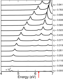
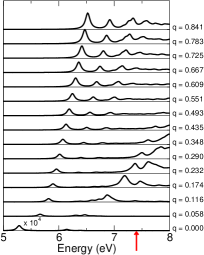
Figure 1: ${\rm Im}\,\epsilon_{M}(\mathbf{q},\omega)$ of (a) graphane and (b) h-BN calculated for several values of $\mathbf{q}$ (in Å^-1) along ${\Gamma}M$. For sake of clarity, each spectrum has been multiplied by $q^{2}$. The red arrows mark the QP band gap.

In Fig. 2 we compare the electronic distribution of the wavefunctions $\Psi^{\lambda}_{\mathbf{q}}(\mathbf{r}_{h},\mathbf{r}_{e})$ for $\mathbf{q}\rightarrow 0$ and $\mathbf{q}=0.4$ Å^-1 of the lowest-energy excitons of graphane and h-BN, fixing the position of the hole where the valence electron wavefunction is mostly localised. This allows one to infer the spatial extension of the exciton from the solution of the BSE, as shown in several 2D materials for $\mathbf{q}\rightarrow 0$ Molina-Sánchez et al. (2013); Cudazzo et al. (2010); Luo et al. (2011); Hsueh et al. (2011); Qiu et al. (2013); sup . In graphane at $\mathbf{q}\rightarrow 0$ the electronic charge, for a hole fixed on a C-C bond, is distributed on both C and H atoms and is delocalized over several unit cells Cudazzo et al. (2010). On the contrary, in h-BN it is strongly localized around the hole, which is placed on the N atom, with a small contribution coming from the nearest-neighbour N atoms. In h-BN the exciton can be hence interpreted as an excitation of a “super atom” encompassing both N and B orbitals. It is localized on N sites due to the strong excitonic effects (for the analogous case of LiF in 3D, see Abbamonte et al. (2008)).

The EBE at $\mathbf{q}\rightarrow 0$ in the two systems is similar: 1.6 eV in graphane and 2.1 eV in h-BN. This is in seeming contrast to the large difference in the exciton wavefunction. It illustrates the fact that in low dimensions the value of the EBE measured in the absorption spectra at $\mathbf{q}\rightarrow 0$ does not directly give information about the nature of the exciton. On the contrary in the 3D case the spatial localization of excitons correlates directly with their binding energy. This allows one to classify excitons in 3D as localized Frenkel excitons with EBEs of the order of several eV, and delocalized Wannier-Mott excitons with EBEs of tens of meV Knox (1963); Bassani and Parravicini (1975). This can be understood, since in 3D semiconductors screening is strong for large distances between electron and hole, which reduces the binding energy of Wannier excitons. In 2D semiconductors the macroscopic screening is much weaker Keldysh (1979); Cudazzo et al. (2011), resulting in a strong increase of their EBE. At short distances instead, screening is always weak in both 2D and 3D, and therefore it does not play a crucial role for the EBE of Frenkel excitons, where electron and hole are close together. Therefore, EBEs of Frenkel excitons are less sensitive to the dimensionality, and similar to the ones of Wannier excitons in 2D.

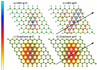
Figure 2: Electronic distribution of the wavefunction $\Psi^{\lambda}_{\mathbf{q}}$ of the lowest-energy exciton of graphane and h-BN for fixed position of the hole (black sphere) calculated for $\mathbf{q}\rightarrow 0$ (left) and 0.4 Å^-1 (right). The black arrow is the direction of $\mathbf{q}\neq 0$. White and green spheres represent N and B atoms in h-BN and H and C atoms in graphane.

In the following, we show that it is nevertheless possible to distinguish different excitons in 2D: the clue is to look at non-vanishing wave vector $\mathbf{q}$. This is illustrated by the wavefunctions in Fig. 2. As $\mathbf{q}$ increases, in h-BN the electronic charge becomes anisotropically delocalized with respect to the position of the hole, but in graphane it is independent of $\mathbf{q}$. This striking result suggests that the exciton band structure $E^{\lambda}_{\mathbf{q}}$, that can also be obtained from experiment, should be analyzed more in detail. Fig. 3(a) shows the calculated band structure of the lowest-energy bright excitons in h-BN and graphane. Its curvature can be classified in two different categories. In h-BN the dispersion is linear for small $\mathbf{q}$ and the curve flattens at large $\mathbf{q}$. In graphane instead $E^{\lambda}_{\mathbf{q}}=E_{\mathbf{q}=0}^{\lambda}+\alpha q^{2}$. The figure also shows the exciton dispersion of phosphorene: it behaves similar to graphane with a parabolic dispersion excluding a very restricted range around $\mathbf{q}=0$ sup .

By a parabolic fit of the exciton dispersion of graphane sup , the effective mass $m_{\textrm{exc}}$ of the dark and bright exciton can be estimated to be 1.6 and 1.8, respectively. Both values match well the sum $m_{e}+m_{h}=1.3$ of the effective electron mass $m_{e}$ and the average value $m_{h}$ of the effective masses of the heavy and light holes at the $\Gamma$ point in the electronic band structure. This result evidences the Wannier character of the exciton in graphane: the dispersion is set by the center-of-mass motion of the e-h pair displaying a free-particle-like behavior (the same holds for phosphorene sup ). This also explains why the exciton wavefunction in graphane is independent of $\mathbf{q}$ (see Fig. 2). When the electron and the hole separately behave as free particles moving in a homogeneous dielectric material (i.e. in the Wannier model), it is possible to find a canonical transformation that decouples the center-of-mass motion from the relative motion of the e-h pair Wannier (1937). In this case the exciton state factorizes in the product of the center-of-mass wavefunction, which propagates as a free particle with momentum $\mathbf{q}$, and an e-h correlation function that is independent of $\mathbf{q}$. The exciton wavefunction thus depends on $\mathbf{q}$ only through a phase factor and does not change its shape as $\mathbf{q}$ increases.

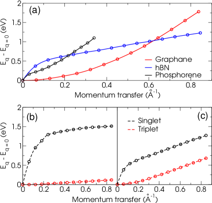
Figure 3: (a) Calculated dispersion of the lowest-energy bright excitons in graphane and h-BN along ${\Gamma}M$ and phosphorene along ${\Gamma}X$. (b) Singlet and triplet exciton dispersion in h-BN in a two-band model with flat bands and (c) with the real electronic band structure.

In order to rationalize the exciton band dispersion in h-BN, we solve the ab initio BSE as above but considering only transitions between the top-valence and the bottom-conduction bands in which we artificially set the dispersion to 0. This corresponds to neglecting the electron and hole hopping terms sup . This choice is suggested by the observation that in h-BN the lowest excited state involves e-h pairs belonging to the $MK$ line of the first Brillouin zone, where the bands have a weak dispersion sup . In such a simplified situation with only two flat bands and assuming a negligible overlap between wavefunctions localized on different atomic sites, the $\mathbf{q}$-dispersion is that of a pure Frenkel exciton, given by Cudazzo et al. (2013b, 2015); sup :

$$E^{\textrm{FR}}_{\mathbf{q}}={\Delta}E+\mathcal{I}(\mathbf{q})-\mathcal{W},$$ (1)

where ${\Delta}E$ is the energy difference between the two flat bands, $\mathcal{W}$ is the on-site term of the direct e-h attraction $W$, and $\mathcal{I}(\mathbf{q})$, which is the only term that can induce a dispersion of the exciton energy, is the excitation-transfer interaction Bassani and Parravicini (1975) related to the exchange e-h repulsion.

Fig. 3(b) displays the lowest-exciton dispersion obtained from the BSE considering the two flat bands in h-BN for both the singlet and triplet channels. We find that the triplet exciton has a negligible dispersion, following the behavior described by Eq. (1), since for the triplet the exchange e-h interaction is absent and thus $\mathcal{I}(\mathbf{q})=0$. This demonstrates that in absence of hopping the lowest excited state of h-BN is a pure Frenkel exciton. In the singlet channel the exciton has a linear dispersion for $\mathbf{q}\rightarrow 0$ and reaches a constant value at large $\mathbf{q}$. This behavior is due to the $\mathbf{q}$-dependence of the exchange e-h repulsion, which at small $\mathbf{q}$ can be described in terms of a dipole-dipole interaction. In this regime, the linearity of $\mathcal{I}(\mathbf{q})$ is in contrast with 3D bulk insulators, where it is generally characterized by a quadratic $\mathbf{q}$-dispersion Cohen and Keffer (1955).

To better understand the effect of the dimensionality on the exchange e-h interaction we consider a quasi-2D dielectric of finite thickness $d$ along the $z$ axis normal to the plane. We assume that the electronic orbitals $\psi(\mathbf{r}$) can be factorized in an in-plane $\phi(\mathbf{\rho})$ and out-of-plane $\chi(z)$ components: $\psi(\mathbf{r})=\phi(\mathbf{\rho})\chi(z)$. With the simplest form $\chi(z)=1/\sqrt{d}$ for $|z|<d/2$ and $\chi(z)=0$ for $|z|>d/2$, i.e. $\chi$ constant inside the 2D slab and zero elsewhere, the exchange e-h interaction gives rise sup to the following dispersion (where we introduce the dipole matrix element $\boldsymbol{\mu}_{vc}$ related to the valence-conduction transition):

$$\mathcal{I}(\mathbf{q})=\frac{4\pi}{d}(\hat{\mathbf{q}}\cdot\boldsymbol{\mu}_{cv})(\hat{\mathbf{q}}\cdot\boldsymbol{\mu}_{vc})\left[1-\frac{1}{qd}(1-e^{-qd})\right],$$ (2)

which is linear for $q\ll 1/d$ and becomes a constant for $q\gg 1/d$ sup . Alternatively, the linear behavior at small $\mathbf{q}$ can be obtained using a 2D Coulomb potential in the evaluation of the exchange e-h interaction Hambach (2010). This means that in the optical limit $\mathbf{q}\rightarrow 0$ the system behaves as a strictly 2D dielectric. At large $\mathbf{q}$, on the other hand, when $1/q$ becomes comparable with $d$, finite-thickness effects become important due to the 3D nature of the Coulomb interaction. The system does not behave anymore as an infinite 2D dielectric, but rather as a 3D finite system . As a consequence, due to the absence of the hopping, at large $\mathbf{q}$ the exciton stops dispersing. This means that the exciton band dispersion displayed in Fig. 3(b) is not materials specific but general, being strictly related to the confinement of the electronic charge in a 2D slab and its effect on the e-h exchange. This interpretation is further confirmed by the fact that the dark exciton along ${\Gamma}M$ does not disperse sup (with $\boldsymbol{\mu}_{vc}=0$ one has $\mathcal{I}(\mathbf{q})=0$).

When we solve the BSE with the real dispersion of the top-valence and bottom-conduction bands [see Fig. 3(c)], the singlet exciton is the same as from the full calculation that takes into account all the bands (see Fig. 3(a)). This confirms that the exciton in h-BN mainly originates from transitions between that pair of bands. The hopping, i.e. the dispersion of the electronic band structure, modifies the dispersion of the singlet exciton with respect to the flat-band limit. Moreover, by taking into account the band dispersion, also the triplet exciton in Fig. 3(c) acquires a dispersion. The correspondence of the triplet exciton and electronic band dispersions sup suggests that the contribution coming from the hopping term is of second or higher order in $\mathbf{q}$, as expected also from a tight-binding description. This also implies that the effect of the hopping on the singlet exciton is negligible in the optical limit, where the dispersion is dominated by the exchange e-h interaction, which is linear in $\mathbf{q}$. On the other hand, at large $\mathbf{q}$ where $\mathcal{I}(\mathbf{q})$ becomes a constant, the dispersion is set only by the hopping in both singlet and triplet channels. Indeed, in Fig. 3(c) we can observe that at large $\mathbf{q}$ triplet and singlet excitons have the same dispersion.

The mechanism at the basis of the spatial delocalization of the exciton in h-BN can be also analogously understood as the effect of the coupling, induced by the hopping, between the pure Frenkel and other more delocalised excitons Cudazzo et al. (2013b, 2015); sup (this is the reason why the exciton in h-BN is delocalised also on nearest-neighbour sites, see Fig. 2). In particular we can distinguish two different mechanisms. The first one is related to the $\mathbf{q}$ dependence of the exciton energy through the exchange e-h interaction [see Eq. (1)]. As $\mathbf{q}$ increases the energy of the pure Frenkel exciton gets closer to the other delocalised excitons (see Fig. 1) enhancing the coupling between them. This causes an isotropic delocalization of the exciton wavefunction. The second effect is related to the explicit $\mathbf{q}$-dependence of the hopping term. As $\mathbf{q}$ increases, this gives rise to the anisotropic delocalization of the exciton wavefunction in h-BN sup that is displayed in Fig. 2.

In conclusion, we have shown that in 2D materials excitons of different character cannot be distinguished by their binding energy, but by their dependence on the exciton wave vector $\mathbf{q}$. Striking differences between Wannier and Frenkel-like excitons are observed in the exciton wavefunction $\Psi^{\lambda}_{\mathbf{q}}$, which is obtained from the numerical solution of the BSE. These differences are also present in the exciton band structure, which can be readily accessed experimentally by momentum-resolved electron energy loss spectroscopy (EELS) Egerton (2011); Wachsmuth (2014) or resonant inelastic X ray spectroscopy (RIXS) Schülke (2007); Ament et al. (2011). Therefore, the present work suggests to use the exciton band structure as a direct and powerful indicator for the exciton character in 2D systems and the relative importance of the different e-h interactions at play in the materials. Our conclusions are supported by numerical results for three prototypical 2D semiconductors. An analysis based on general arguments shows the the findings are not materials specific, but generally valid for all 2D materials.

This research was supported by the European Research Council (ERC Grant Agreement n. 320971) and by a Marie Curie FP7 Integration Grant within the 7th European Union Framework Programme. Computational time was granted by GENCI (Project No. 544).

References

- Novoselov et al. (2005a) K. S. Novoselov, A. K. Geim, S. V. Morozov, D. Jiang, M. I. Katsnelson, I. V. Grigorieva, S. V. Dubonos, and A. A. Firsov, Nature 438, 197 (2005a).
- Castro Neto et al. (2009) A. H. Castro Neto, F. Guinea, N. M. R. Peres, K. S. Novoselov, and A. K. Geim, Rev. Mod. Phys. 81, 109 (2009).
- Zhang et al. (2005) Y. Zhang, Y.-W. Tan, H. L. Stormer, and P. Kim, Nature 438, 201 (2005).
- Novoselov et al. (2007) K. S. Novoselov, Z. Jiang, Y. Zhang, S. V. Morozov, H. L. Stormer, U. Zeitler, J. C. Maan, G. S. Boebinger, P. Kim, and A. K. Geim, Science 315, 1379 (2007).
- Mak et al. (2010) K. F. Mak, C. Lee, J. Hone, J. Shan, and T. F. Heinz, Phys. Rev. Lett. 105, 136805 (2010).
- Splendiani et al. (2010) A. Splendiani, L. Sun, Y. Zhang, T. Li, J. Kim, C.-Y. Chim, G. Galli, and F. Wang, Nano Letters 10, 1271 (2010).
- Xiao et al. (2012) D. Xiao, G.-B. Liu, W. Feng, X. Xu, and W. Yao, Phys. Rev. Lett. 108, 196802 (2012).
- Mak et al. (2012) K. F. Mak, K. He, J. Shan, and T. F. Heinz, Nat Nano 7, 494 (2012).
- Zeng et al. (2012) H. Zeng, J. Dai, W. Yao, D. Xiao, and X. Cui, Nat Nano 7, 490 (2012).
- Cao et al. (2012) T. Cao, G. Wang, W. Han, H. Ye, C. Zhu, J. Shi, Q. Niu, P. Tan, E. Wang, B. Liu, and J. Feng, Nat Commun 3, 887 (2012).
- Wang et al. (2012) Q. H. Wang, K. Kalantar-Zadeh, A. Kis, J. N. Coleman, and M. S. Strano, Nat Nano 7, 699 (2012).
- Xu et al. (2014) X. Xu, W. Yao, D. Xiao, and T. F. Heinz, Nat Phys 10, 343 (2014).
- Yu et al. (2014) H. Yu, G.-B. Liu, P. Gong, X. Xu, and W. Yao, Nat Commun 5, (2014).
- Li et al. (2014) Y. Li, J. Ludwig, T. Low, A. Chernikov, X. Cui, G. Arefe, Y. D. Kim, A. M. van der Zande, A. Rigosi, H. M. Hill, S. H. Kim, J. Hone, Z. Li, D. Smirnov, and T. F. Heinz, Phys. Rev. Lett. 113, 266804 (2014).
- MacNeill et al. (2015) D. MacNeill, C. Heikes, K. F. Mak, Z. Anderson, A. Kormányos, V. Zólyomi, J. Park, and D. C. Ralph, Phys. Rev. Lett. 114, 037401 (2015).
- Srivastava et al. (2015) A. Srivastava, M. Sidler, A. V. Allain, D. S. Lembke, A. Kis, and A. Imamoglu, Nat Phys 11, 141 (2015).
- Aivazian et al. (2015) G. Aivazian, Z. Gong, A. M. Jones, R.-L. Chu, J. Yan, D. G. Mandrus, C. Zhang, D. Cobden, W. Yao, and X. Xu, Nat Phys 11, 148 (2015).
- Xia et al. (2014) F. Xia, H. Wang, D. Xiao, M. Dubey, and A. Ramasubramaniam, Nat Photon 8, 899 (2014).
- Liu et al. (2015) X. Liu, T. Galfsky, Z. Sun, F. Xia, E.-c. Lin, Y.-H. Lee, S. Kéna-Cohen, and V. M. Menon, Nat Photon 9, 30 (2015).
- Wirtz et al. (2006) L. Wirtz, A. Marini, and A. Rubio, Phys. Rev. Lett. 96, 126104 (2006).
- Molina-Sánchez et al. (2013) A. Molina-Sánchez, D. Sangalli, K. Hummer, A. Marini, and L. Wirtz, Phys. Rev. B 88, 045412 (2013).
- Cudazzo et al. (2010) P. Cudazzo, C. Attaccalite, I. V. Tokatly, and A. Rubio, Phys. Rev. Lett. 104, 226804 (2010).
- Luo et al. (2011) G. Luo, X. Qian, H. Liu, R. Qin, J. Zhou, L. Li, Z. Gao, E. Wang, W.-N. Mei, J. Lu, Y. Li, and S. Nagase, Phys. Rev. B 84, 075439 (2011).
- Hsueh et al. (2011) H. C. Hsueh, G. Y. Guo, and S. G. Louie, Phys. Rev. B 84, 085404 (2011).
- Qiu et al. (2013) D. Y. Qiu, F. H. da Jornada, and S. G. Louie, Phys. Rev. Lett. 111, 216805 (2013).
- Chernikov et al. (2014) A. Chernikov, T. C. Berkelbach, H. M. Hill, A. Rigosi, Y. Li, O. B. Aslan, D. R. Reichman, M. S. Hybertsen, and T. F. Heinz, Phys. Rev. Lett. 113, 076802 (2014).
- He et al. (2014) K. He, N. Kumar, L. Zhao, Z. Wang, K. F. Mak, H. Zhao, and J. Shan, Phys. Rev. Lett. 113, 026803 (2014).
- Hanbicki et al. (2015) A. Hanbicki, M. Currie, G. Kioseoglou, A. Friedman, and B. Jonker, Solid State Communications 203, 16 (2015).
- Wang et al. (2015) X. Wang, A. M. Jones, K. L. Seyler, V. Tran, Y. Jia, H. Zhao, H. Wang, L. Yang, X. Xu, and F. Xia, Nat Nano 10, 517 (2015).
- Zeppenfeld (1971) K. Zeppenfeld, Zeitschrift für Physik 243, 229 (1971).
- Marinopoulos et al. (2004) A. G. Marinopoulos, L. Reining, A. Rubio, and V. Olevano, Phys. Rev. B 69, 245419 (2004).
- Wachsmuth et al. (2014) P. Wachsmuth, R. Hambach, G. Benner, and U. Kaiser, Phys. Rev. B 90, 235434 (2014).
- Kramberger et al. (2008) C. Kramberger, R. Hambach, C. Giorgetti, M. H. Rümmeli, M. Knupfer, J. Fink, B. Büchner, L. Reining, E. Einarsson, S. Maruyama, F. Sottile, K. Hannewald, V. Olevano, A. G. Marinopoulos, and T. Pichler, Phys. Rev. Lett. 100, 196803 (2008).
- Wachsmuth et al. (2013) P. Wachsmuth, R. Hambach, M. K. Kinyanjui, M. Guzzo, G. Benner, and U. Kaiser, Phys. Rev. B 88, 075433 (2013).
- Liou et al. (2015) S. C. Liou, C.-S. Shie, C. H. Chen, R. Breitwieser, W. W. Pai, G. Y. Guo, and M.-W. Chu, Phys. Rev. B 91, 045418 (2015).
- van Wezel et al. (2011) J. van Wezel, R. Schuster, A. König, M. Knupfer, J. van den Brink, H. Berger, and B. Büchner, Phys. Rev. Lett. 107, 176404 (2011).
- Cudazzo et al. (2012) P. Cudazzo, M. Gatti, and A. Rubio, Phys. Rev. B 86, 075121 (2012).
- Faraggi et al. (2012) M. N. Faraggi, A. Arnau, and V. M. Silkin, Phys. Rev. B 86, 035115 (2012).
- Cudazzo et al. (2013a) P. Cudazzo, M. Gatti, and A. Rubio, New Journal of Physics 15, 125005 (2013a).
- Soininen and Shirley (2000) J. A. Soininen and E. L. Shirley, Phys. Rev. B 61, 16423 (2000).
- Abbamonte et al. (2008) P. Abbamonte, T. Graber, J. P. Reed, S. Smadici, C.-L. Yeh, A. Shukla, J.-P. Rueff, and W. Ku, Proc. Natl. Acad. Sci. 105, 12159 (2008).
- Lee et al. (2013) C.-C. Lee, X. M. Chen, Y. Gan, C.-L. Yeh, H. C. Hsueh, P. Abbamonte, and W. Ku, Phys. Rev. Lett. 111, 157401 (2013).
- Gatti and Sottile (2013) M. Gatti and F. Sottile, Phys. Rev. B 88, 155113 (2013).
- Cudazzo et al. (2013b) P. Cudazzo, M. Gatti, A. Rubio, and F. Sottile, Phys. Rev. B 88, 195152 (2013b).
- Elias et al. (2009) D. C. Elias, R. R. Nair, T. M. G. Mohiuddin, S. V. Morozov, P. Blake, M. P. Halsall, A. C. Ferrari, D. W. Boukhvalov, M. I. Katsnelson, A. K. Geim, and K. S. Novoselov, Science 323, 610 (2009).
- Liu et al. (2014) H. Liu, A. T. Neal, Z. Zhu, Z. Luo, X. Xu, D. Tománek, and P. D. Ye, ACS Nano 8, 4033 (2014), pMID: 24655084, http://dx.doi.org/10.1021/nn501226z .
- Novoselov et al. (2005b) K. S. Novoselov, D. Jiang, F. Schedin, T. J. Booth, V. V. Khotkevich, S. V. Morozov, and A. K. Geim, Proc. Natl. Acad. Sci. 102, 10451 (2005b).
- Jin et al. (2009) C. Jin, F. Lin, K. Suenaga, and S. Iijima, Phys. Rev. Lett. 102, 195505 (2009).
- Alem et al. (2009) N. Alem, R. Erni, C. Kisielowski, M. D. Rossell, W. Gannett, and A. Zettl, Phys. Rev. B 80, 155425 (2009).
- Onida et al. (2002) G. Onida, L. Reining, and A. Rubio, Rev. Mod. Phys. 74, 601 (2002).
- Hedin (1965) L. Hedin, Phys. Rev. 139, A796 (1965).
- (52) See Supplementary Material for computational details and for additional spectra and analysis.
- Ismail-Beigi (2006) S. Ismail-Beigi, Phys. Rev. B 73, 233103 (2006).
- Marini et al. (2009) A. Marini, C. Hogan, M. Grüning, and D. Varsano, Computer Physics Communications 180, 1392 (2009).
- Sponza (2013) L. Sponza, Ph.D. thesis, Ecole Polytechnique, Palaiseau (France) (2013).
- Knox (1963) R. S. Knox, Theory of Excitons (Academic Press, 1963).
- Bassani and Parravicini (1975) F. Bassani and G. P. Parravicini, Electronic States and Optical Transitions in Solids (Pergamon Press, 1975).
- Keldysh (1979) L. Keldysh, JETP Lett. 29, 658 (1979).
- Cudazzo et al. (2011) P. Cudazzo, I. V. Tokatly, and A. Rubio, Phys. Rev. B 84, 085406 (2011).
- Wannier (1937) G. H. Wannier, Phys. Rev. 52, 191 (1937).
- Cudazzo et al. (2015) P. Cudazzo, F. Sottile, A. Rubio, and M. Gatti, Journal of Physics: Condensed Matter 27, 113204 (2015).
- Cohen and Keffer (1955) M. H. Cohen and F. Keffer, Phys. Rev. 99, 1128 (1955).
- Hambach (2010) R. Hambach, Ph.D. thesis, Ecole Polytechnique, Palaiseau (France) (2010).
- Note (1) A similar effect of the finite thickness can be found also on the intraband plasmon dispersion of 2D metals Ritchie (1957); Ferrell (1958).
- Egerton (2011) R. Egerton, Electron Energy-Loss Spectroscopy in the Electron Microscope (Springer, 2011).
- Wachsmuth (2014) P. Wachsmuth, Ph.D. thesis, Ulm University, (Germany) (2014).
- Schülke (2007) W. Schülke, Electron Dynamics by Inelastic X-Ray Scattering, Oxford Series on Synchrotron Radiation (Oxford Univ. Press, Oxford, 2007).
- Ament et al. (2011) L. J. P. Ament, M. van Veenendaal, T. P. Devereaux, J. P. Hill, and J. van den Brink, Rev. Mod. Phys. 83, 705 (2011).
- Ritchie (1957) R. H. Ritchie, Phys. Rev. 106, 874 (1957).
- Ferrell (1958) R. A. Ferrell, Phys. Rev. 111, 1214 (1958).