Can Dark Matter be an artifact of extended theories of gravity?

Abstract

In this article, we propose different background models of extended theories of gravity, which are minimally coupled to the SM fields, to explain the possibility of genesis of dark matter without affecting the SM particle sector. We modify the gravity sector by allowing quantum corrections motivated from (1) local $f(R)$ gravity and (2) non-minimally coupled gravity with SM sector and dilaton field. Next we apply conformal transformation on the metric to transform the action back to the Einstein frame. We also show that an effective theory constructed from these extended theories of gravity and SM sector looks exactly the same. Using the relic constraint observed by Planck 2015, we constrain the scale of the effective field theory ($\Lambda_{UV}$) as well as the dark matter mass ($M$). We consider two cases- (1) light dark matter (LDM) and (2) heavy dark matter (HDM), and deduce upper bounds on thermally averaged cross section of dark matter annihilating to SM particles. Further we show that our model naturally incorporates self interactions of dark matter. Using these self interactions, we derive the constraints on the parameters of the (1) local $f(R)$ gravity and (2) non-minimally coupled gravity from dark matter self interaction. Finally, we propose some different UV complete models from a particle physics point of view, which can give rise to the same effective theory that we have deduced from extended theories of gravity.

1 Introduction

Different cosmological measurements have confirmed that majority of the matter in this universe occurs in the form of a non-luminous “dark matter”(DM). Infact DM accounts for almost $30\%$ of the energy budget of the universe Komatsu . Experimentally measured relic density of DM gives us some insights into the particle nature of DM. It is a very well known fact that Standard Model (SM) of particle physics cannot provide any dark matter candidate. It is believed that to search for the existence of dark matter candidate, physics Beyond Standard Model (BSM) is necessary Jungman ; Bergstrom:2000pn ; Feng:2010gw . These extensions of the SM are strongly motivated from observations of the galactic rotation curves, motion of galaxy clusters, two colliding clusters of galaxies in the Bullet Cluster and cosmological observations Clowe:2006eq . In such a scenario, the matter sector is modified without affecting the gravity sector. But more precisely this type of approach is mostly ad-hoc as it does not always provide any theoretical origin of such extensions in the matter sector (with the exceptions of a few DM models like neutralino WIMP, axion etc.). Alternatively these observations have also been explained through modification of the gravity sector without the need of any dark matter candidate, for example: Modified Newtonian dynamics (MOND) paradigm Milgrom:2009an and Tensor-vector-scalar gravity (TeVeS) Bekenstein:2004ne . But such proposals are not consistent with all the observational constraints . To avoid the ambiguity of ad-hoc extensions of the SM, in this paper we propose an alternative framework based on the principles of Effective Field Theory (EFT) Busoni:2013lha ; Busoni:2014sya ; Busoni:2014haa ; Macias:2015cna ; Beltran:2008xg ; Goodman:2010yf ; Goodman:2010ku ; Goodman:2010qn ; Fan:2010gt ; Cheung:2010ua ; Cheung:2011nt ; Cheung:2012gi ; Fitzpatrick:2012ix ; Kumar:2013iva ; DeSimone:2013gj . In this EFT approach, we represent the interactions between DM and SM through a set of higher dimensional effective non-renormalizable Wilsonian operators, which are generated by integrating out the heavy mediator degrees of freedom at higher scales. This approach works best when there is a clear separation of energy scales between the ultraviolet physics, and the relevant energy scales. This is clearly the case here, because when we consider indirect detection of DM, where two DM particles annihilate to two SM particles, the momentum transferred in the process is of the order of the DM mass, which is clearly less than the energy scales considered. Even in case of direct detection, the momentum transferred in a collision with a nuclei, is of the order of a few keV. This justifies the use of an EFT.

We start with the extended version of gravity sector keeping the SM matter sector unchanged. Such modifications in the gravity sector usually originates from quantum corrections in the gravity sector and are motivated from various background higher dimensional field theoretic setups . One can also consider modification in the gravity sector by allowing non-minimal interaction between the matter field and gravity . In the present context we use conformal transformation on the metric to explain the genesis of scalar dark matter from various types of extended theories of gravity, i.e., local $f(R)$ gravity felice:2010 ; Sotiriou:2008rp  , non-local theories of gravity Biswas:2011ar ; Biswas:2012bp ; Biswas:2013kla ; Biswas:2013cha ; Chialva:2014rla ; Conroy:2014eja ; Talaganis:2014ida ; Conroy:2015wfa ; Conroy:2015nva   and finally we also allow non-minimal interaction between Einstein gravity with scalar matter field Bezrukov:2010jz ; Bezrukov:2012hx ; GarciaBellido:2012zu ; GarciaBellido:2011de ; Shaposhnikov:2009pv ; Bezrukov:2009db ; Bezrukov:2008ej ; Bezrukov:2007ep ; Choudhury:2013zna ; Salvio:2015kka as mentioned earlier. Thus in our prescribed methodology, although we start with an unchanged matter sector, it gets modified because of modifications in the gravity sector. This is where we differ from the contemporary ideas. Further to implement the constraint from observational probes  on the relic density of the dark matter we use the tools and techniques of Effective Field Theory in the present setup.

Throughout the analysis of the paper we use the following sets of crucial assumptions:

1. We use the tools and techniques of the Effective Field Theory in the present context while applying the constraints from observational probes and indirect detection experiments. Instead of introducing a Planckian cut-off at $M_{p}\sim 10^{19}~{}{\rm{\rm GeV}}$ here, we introduce a new UV cut-off scale, $\Lambda_{UV}<<M_{p}$ of the Effective Field Theory. In principle, more precisely this can be treated as the tuning parameter of the theoretical setup and we have shown explicitly from our prescribed analysis that this serves a very crucial role to satisfy the constraint for dark matter relic abundance as obtained from Planck 2015 Ade:2015xua data.

2. We are implementing our prescribed methodology by taking some of the few well known examples of extended theories of gravity, i.e., local $f(R)$ gravity and non-minimally coupled gravity with scalar matter, in which, by applying conformal transformation on the metric one is able to construct a reduced and easier version of the theory in Einstein frame in terms of Einstein gravity, a new scalar matter field (dilaton) and an interaction between SM sector and dilaton matter field. In our prescription, we identify such a dilaton field to be the dark matter candidate.

3. To validate to perturbative approximation appropriately in the present context we also assume that the interaction between SM sector and dilaton matter field is weak. Consequently, we expand the exponential dilaton coupling and due to large suppression by the cut-off scale $\Lambda_{UV}$, we only take first three terms in the expansion series.

4. Next we additionally impose a ${\cal Z}_{2}$ symmetry on dilaton, and drop the odd term under this symmetry. As a result here we have only the first term ${\cal L}_{SM}$ and third term $\frac{\phi^{2}}{\Lambda^{2}_{UV}}{\cal L}_{SM}$. In our paper, the third term $\frac{\phi^{2}}{\Lambda^{2}_{UV}}{\cal L}_{SM}$ plays the significant role to describe the genesis of dilaton dark matter. One loop corrections to the dilaton mass puts an upper limit of $M\leq 4\pi\Lambda_{UV}$ Blum:2014jca ; Gannouji:2012iy .

5. During our analysis we also assume that annihilation of DM at the galactic centre proceeds with a velocity $v\approx 10^{-3}$. Consequently the thermally averaged cross- section $\langle\sigma v\rangle$ is expanded in terms $s$-wave and $p$-wave contributions. We neglect all other higher order contributions in $\langle\sigma v\rangle$.

6. Most importantly, in our prescribed methodology we assume the non-relativistic ($NR$) limit to compute and also expand the expression for the thermally averaged cross- section $\langle\sigma v\rangle$.

7. In our analysis, we consider maximum mass of the dilaton dark matter to be ${\cal O}(1~{}{\rm TeV})$. But our conclusions will remain unchanged for higher masses, as long as they satisfy the relic density constraint. Higher the mass we consider, larger will be the scale of our effective theory.

The plan of the paper is as follows.

• In section 2, we propose background models of extended theories of gravity, which are minimally coupled to SM fields. Initially we start with a model where the usual Einstein gravity is minimally coupled with the SM sector. But such a theory is not able to explain the genesis of dark matter at all. To explain this possibility without affecting the SM particle sector, we modify the gravity sector by allowing quantum corrections motivated from (1) local $f(R)$ gravity and (2) non-minimally coupled dilaton with gravity and SM sector.

• In section 3, we construct our theory in the Einstein frame by applying conformal transformation on the metric. We explicitly discuss the rules and detailed techniques of conformal transformation in the gravity sector as well as in the matter sector. For completeness, we present the results for arbitrary $D$ space-time dimensions. We use $D=4$ in the rest of our analysis. Then we also show that the effective theory constructed from (1) local $f(R)$ gravity and (2) non-minimally coupled dilaton with gravity and SM sector looks exactly same. Through conformal transformation, we derive the explicit form of dilaton effective potentials, which will be helpful to study the self interaction properties of the dark matter as well as the signatures of inflationary paradigm. In this paper, we have not explored this possibility. Detailed calculations are shown in section 8 (Appendix A).

• In section 4, we use the relic constraint as observed by Planck 2015 to constrain the scale of the effective field theory $\Lambda_{UV}$ as well as the dark matter mass $M$. We consider two cases- (1) light dark matter (LDM) and (2) heavy dark matter (HDM), and deduce upper bounds on thermally averaged cross section of dark matter annihilating to SM particles, in the non-relativistic limit. This classification of DM into HDM and LDM is purely on the basis of the scale of the EFT considered. For LDM, the maximum mass of the DM candidate considered is less than ${\cal O}(350{\rm GeV})$. For HDM, DM masses between $350~{}{\rm GeV}$ and $1~{}TeV$ are considered. We shall find that for masses of DM greater than $350~{}{\rm GeV}$, the scale of the EFT increases by an order of magnitude, thereby leading to extra suppression.

• In section 5, we explicitly discuss about the constraints on the parameters of the background models of extended theories of gravity- (1) local $f(R)$ gravity and (2) non-minimally coupled dilaton with gravity, by applying the constraints from dark matter self interaction. To describe this fact we consider the process $\phi\phi\rightarrow\phi\phi$, where $\phi$ is the scalar dark matter candidate in Einstein frame as introduced earlier by applying conformal transformation in the metric. Here $\phi\phi\rightarrow\phi\phi$ represents dark matter self-interaction and characterized by the coefficient of $\phi^{4}$ term in the effective potential $V^{{}^{\prime\prime\prime\prime}}_{0}$.

• In section 6, we propose different UV complete models from a particle physics point of view, which can give rise to the same effective theory that we have deduced from extended theories of gravity. We mainly consider two models- (1) Inert Higgs Doublet model for LDM and (2) Inert Higgs Doublet model with a new heavy scalar for HDM. Thus, we have shown that UV completion of this effective theory need not come from modifications to the matter sector, but rather from extensions of the gravity sector.

• In section 7, we conclude with future prospects from this present work.

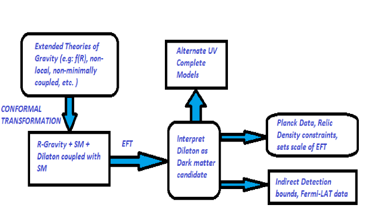
Figure 1: Schematic representation of the setup which shows the complete algorithm of the described methodology in this paper.

2 The background model

In this section we start with the situation, where the well known Standard Model (SM) of particle physics in the matter sector is minimally coupled with the Einstein gravity sector and is described the following effective actionSotiriou:2008rp :

$$S=\int d^{4}x\sqrt{-g}\left[\frac{\Lambda^{2}_{UV}}{2}R+{\cal L}_{SM}\right],$$ (1)

where $R$ is the Ricci scalar, ${\cal L}_{SM}$ is the SM Lagrangian density and $\Lambda_{UV}$ is the UV cut-off of the Effective Filed Theory as mentioned in the introduction of the paper . But it is important to mention here that, the effective action stated in Eq (1) cannot explain the generation of a dark matter candidate without modifying the SM sector.

To solve this problem, one needs to allow extensions in the standard Einstein gravity sector:

1. By adding higher derivative and curvature terms in the effective action. For an example, within the framework of Effective Field Theory, one can incorporate local corrections in General Relativity (GR) in the gravity sector and write the action as ,

   $$S_{local}=\int d^{4}x\sqrt{-\!g}\left[\sum^{\infty}_{n=1}{\bf a}_{n}R^{n}+\sum^{\infty}_{m=1}{\bf b}_{m}\left(R_{\mu\nu}R^{\mu\nu}\right)^{m}+\sum^{\infty}_{p=1}{\bf c}_{p}\left(R_{\alpha\beta\delta\eta}R^{\alpha\beta\delta\eta}\right)^{p}\right].$$ (2)

   The co-efficients ${\bf a_{n}},{\bf b_{m}},{\bf c_{p}}$ of the correction factors affects the ultraviolet behaviour of the gravity theory. But any arbitrary local modification of the renormalizable theory of GR typically contains massive ghosts which cannot be regularized using any standard field theoretic prescriptions. $f(R)$ gravity is one of the simplest versions of extended theory of gravity in which one fixes ${\bf a_{n}}\neq 0,{\bf b_{m}}=0$ and ${\bf c_{p}}=0$. Consequently, the effective action assumes the following simplified form:

   $$S_{local}=\int d^{4}x\sqrt{-\!g}f(R),$$ (3)

   where in general $f(R)$ is given by the following expression:

   $$f(R)=\sum^{\infty}_{n=1}{\bf a}_{n}R^{n},$$ (4)

   which contains the full expansion in the gravity sector in terms of the Ricci scalar $R$. In principle, one can allow any combination of $f(R)$, but to maintain renormalizability in the gravity sector, it is necessary to truncate the above infinite series in finite way. String theory is one of the major sources through which it is possible to generate these types of corrections to the Einstein gravity sector by allowing quantum gravity effects.

2. Considering non-minimal coupling between the Einstein gravity and additional scalar field, one can serve a similar purpose. Firstly, in the matter sector we incorporate the effects of quantum correction through the interaction between heavy and light sector and then integrate out the heavy degrees of freedom from the Effective Field Theory picture. This finally allows an expansion within the light sector, which can be written as:

   $$\begin{array}[]{llll}\displaystyle S_{M}[\phi,\Psi]=\int d^{4}x\sqrt{-^{(4)\!}g}\left[{\cal L}[\phi]+{\cal L}_{Heavy}[\Psi]+{\cal L}_{Int}[\phi,\Psi]\right]\\ \displaystyle~{}~{}\underrightarrow{Integrate~{}~{}out~{}~{}\Psi~{}}~{}~{}~{}e^{iS_{M}[\phi]}=\int[{\cal D}\Psi]e^{iS_{M}[\phi,\Psi]}\\ \displaystyle S_{M}[\phi]=\int d^{4}x\sqrt{-^{(4)\!}g}\left[{\cal L}[\phi]+\sum_{\alpha}J_{\Delta_{\alpha}}(g)\frac{{\cal O}_{\alpha}[\phi]}{\Lambda^{\Delta_{\alpha}-4}_{UV}}\right]\end{array}$$ (5)

   where $J_{\alpha}(g)\forall\alpha$ are the Wilson coefficients which depend on the couplings $g$ of the full theory, and ${\cal O}_{\alpha}[\phi]$ are local operators having dimension $\Delta_{\alpha}$. All possible effective operators ${\cal O}_{\alpha}[\phi]$, which respect the symmetries of the full theory can be generated by this method. ${\cal L}[\phi]$ and ${\cal L}_{Heavy}[\Psi]$ describe the section which involves the light and heavy degrees of freedom, and ${\cal L}_{int}[\phi,\Psi]$ consists of all interactions amongst both sets of fields within Effective Field Theory prescription. After integrating out the heavy fields, the effective action has a renormalizable part:

   $${\cal L}[\phi]=-\frac{g^{\mu\nu}}{2}(\partial_{\mu}\phi)(\partial_{\nu}\phi)-V_{ren}(\phi)$$ (6)

   and a sum of non-renormalizable corrections denoted by ${\cal O}_{\alpha}[\phi]$, as given in Eq. (5). Operators having dimensions less than four are called “relevant operators” while those with dimensions greater than four are called “irrelevant operators”. Theories having higher dimensional operators are dimensionally reduced to a four dimensional Effective Field Theory via various compactifications in string theory sector. However, corrections coming from graviton loops will suppressed by the cut-off scale $\Lambda_{UV}$ which is fixed at Planck scale $M_{p}$, while those arising heavy sector will be suppressed by the background scale relevant for fields whose mass $M_{s}<\Lambda_{UV}\approx M_{p}$. Present observational status limits this scale around the GUT scale ($10^{16}$ GeV). In this context, we assume that the UV scale suppressed operators will only modify the structure of the effective potential, without affecting the kinetic terms in the effective action. Consequently, these corrections will add with the renormalizable part of the potential $V_{ren}$ and give rise to the total potential $V(\phi)$ given by:

   $$V(\phi)=V_{ren}(\phi)+\sum^{\infty}_{\Delta_{\alpha}=5}J_{\Delta_{\alpha}}(g)\frac{\phi^{\Delta_{\alpha}}}{\Lambda^{\Delta_{\alpha}-4}_{UV}}=\sum^{\infty}_{\Delta_{\alpha}=0}C_{\Delta_{\alpha}}(g)\frac{\phi^{\Delta_{\alpha}}}{\Lambda^{\Delta_{\alpha}-4}_{UV}},$$ (7)

   where $C_{\Delta_{\alpha}}$s are the Wilson coefficients. Thus the effective Lagrangian for the $\phi$ field is modified as:

   $${\cal L}[\phi]=-\frac{g^{\mu\nu}}{2}(\partial_{\mu}\phi)(\partial_{\nu}\phi)-V(\phi).$$ (8)

Taking all these into account, the effective action for the background model can be expressed as:

$$\begin{array}[]{lll}\displaystyle S=\left\{\begin{array}[]{lll}\displaystyle\int d^{4}x\sqrt{-g}\left[\frac{\Lambda^{2}_{UV}}{2}f(R)+{\cal L}_{SM}\right]\,,{}{}{}{}{}{}&\mbox{\small{\bf for {Case I }}}\\ \displaystyle\int d^{4}x\sqrt{-g}\left[\frac{\Lambda^{2}_{UV}}{2}\left(1+\xi\frac{\phi^{2}}{\Lambda^{2}_{UV}}\right)R+{\cal L}[\phi]+{\cal L}_{SM}\right]{}{}{}{}{}{}&\mbox{\small{\bf for {Case II}}}\end{array}\right.\end{array}$$ (9)

where for Case I, $f(R)$ represents any function of $R$ in general  and for Case II, $\phi$ is the additional scalar field coupled to $R$ via non-minimal coupling $\xi$ . Here for all three cases $\Lambda_{UV}$ represents the Ultra-Violet (UV) cut-off scale for the Effective Field Theory. In this article, we will follow all possibilities with which we can study the effective theory of dark matter in detail. It is important to mention here that, all the effective actions are constructed in the Jordan frame of gravity. To explain the genesis of dark matter from the effective action, we have to apply conformal transformation in the metric, which transform the Jordan frame gravity to the Einstein frame. In the next section we discuss the technical details of conformal transformation in the extended gravity sector.

3 Construction of effective models from extended theories of gravity in Einstein frame

Conformal transformation of the metric is an appealing characteristic of the scalar-tensor theory of gravity Kanno:2002ia which originates from superstring theory. Using this transformation, one can express the theory in two conformally related frames- Jordan and Einstein frames. In this paper, we use the Einstein frame to explain scalar dark matter generation in the context of Effective Field Theory. In the Einstein frame the new scalar field is coupled with the SM degrees of freedom via a conformal coupling factor. This new scalar field, aka “scalaron” or “dilaton”, has a geometrical origin and is generated from the extended version of the gravity sector through conformal transformation in Einstein frame. In this section, we quote the results for dimension $D=4$, which will be used for further computation in the present context. The details of conformal transformation in arbitrary $D$ dimensions in explicitly computed in section 8 (Appendix A).

3.1 Case I: From $f(R)$ gravity

In case of $f(R)$ gravity, the conformal factor is given by:

$$\Omega(x)=e^{\omega(x)}=e^{\frac{1}{\sqrt{6}}\frac{\phi(x)}{\Lambda_{UV}}}=\sqrt{f^{{}^{\prime}}(R)},$$ (10)

where $\phi$ is known as the “scalaron” or “dilaton”. Here we start with the following action in Jordan frame:

$$\begin{array}[]{lll}\displaystyle S=\int d^{4}x\sqrt{-g}\left[\frac{\Lambda^{2}_{UV}}{2}f(R)+{\cal L}_{SM}\right]\end{array}$$ (11)

which can be recast in the following form:

$$\begin{array}[]{lll}\displaystyle S=\int d^{4}x\sqrt{-g}\left[\frac{\Lambda^{2}_{UV}}{2}f^{{}^{\prime}}(R)R-U+{\cal L}_{SM}\right],\end{array}$$ (12)

where $U$ is defined as:

$$U=\frac{\Lambda^{2}_{UV}}{2}\left[f^{{}^{\prime}}(R)R-f(R)\right].$$ (13)

Now transforming the Jordan frame action into Einstein frame we get finally:

$$S\Longrightarrow\tilde{S}=\int d^{4}x\sqrt{-\tilde{g}}\left[\frac{\Lambda^{2}_{UV}}{2}\tilde{R}-\frac{1}{2}\tilde{g}^{\mu\nu}\partial_{\mu}\phi\partial_{\nu}\phi-V(\phi)+e^{-\frac{2\sqrt{2}}{\sqrt{3}}\frac{\phi}{\Lambda_{UV}}}{\cal L}_{SM}\right],$$ (14)

where the effective potential in Einstein frame is given by:

$$V(\phi)=\frac{U}{(f^{{}^{\prime}}(R))^{2}}=\frac{\Lambda^{2}_{UV}}{2}\frac{f^{{}^{\prime}}(R)R-f(R)}{(f^{{}^{\prime}}(R))^{2}}.$$ (15)

For the further computation we will take the following structures of the function $f(R)$ as :

$$\begin{array}[]{lll}\displaystyle f(R)=aR+bR^{n}=\left\{\begin{array}[]{lll}\displaystyle aR+bR^{2}\,,{}{}{}{}{}{}&\mbox{\small{\bf with {Case A1: $a\neq 0,b\neq 0,n=2$ }}}\\ \displaystyle bR^{2}\,,{}{}{}{}{}{}&\mbox{\small{\bf with {Case B1: $a=0,b\neq 0,n=2$ }}}\\ \displaystyle aR+bR^{n}{}{}{}{}{}{}&\mbox{\small{\bf with {Case C1: $a\neq 0,b\neq 0,n>2$ }}}\end{array}\right.\end{array}$$ (16)

Now using Eq (16) in Eq (10) we get:

$$\begin{array}[]{lll}\displaystyle\Omega(x)=e^{\omega(x)}=e^{\frac{1}{\sqrt{6}}\frac{\phi(x)}{\Lambda_{UV}}}=\left\{\begin{array}[]{lll}\displaystyle\sqrt{\left(a+2bR\right)}\,,{}{}{}{}{}{}&\mbox{\small{\bf with {Case A1: $a\neq 0,b\neq 0,n=2$ }}}\\ \displaystyle\sqrt{2bR}\,,{}{}{}{}{}{}&\mbox{\small{\bf with {Case B1: $a=0,b\neq 0,n=2$ }}}\\ \displaystyle\sqrt{a+nbR^{n-1}},{}{}{}{}{}{}&\mbox{\small{\bf with {Case C1: $a\neq 0,b\neq 0,n>2$ }}}\end{array}\right.\end{array}$$ (17)

where $R$ is the Ricci scalar in Jordan frame.

Further reverting Eq (17) as:

$$\begin{array}[]{lll}\displaystyle R=\left\{\begin{array}[]{lll}\displaystyle\frac{1}{2b}\left(e^{\frac{2}{\sqrt{6}}\frac{\phi(x)}{\Lambda_{UV}}}-a\right)\,,{}{}{}{}{}{}&\mbox{\small{\bf with {Case A1: $a\neq 0,b\neq 0,n=2$ }}}\\ \displaystyle\frac{1}{2b}e^{\frac{2}{\sqrt{6}}\frac{\phi(x)}{\Lambda_{UV}}}\,,{}{}{}{}{}{}&\mbox{\small{\bf with {Case B1: $a=0,b\neq 0,n=2$ }}}\\ \displaystyle\left\{\frac{1}{nb}\left(e^{\frac{2}{\sqrt{6}}\frac{\phi(x)}{\Lambda_{UV}}}-a\right)\right\}^{\frac{1}{n-1}},{}{}{}{}{}{}&\mbox{\small{\bf with {Case C1: $a\neq 0,b\neq 0,n>2$ }}}\end{array}\right.\end{array}$$ (18)

and also using Eq (18) in Eq (15), the effective potential can be expressed as:

$$\begin{array}[]{lll}\displaystyle V(\phi)=\left\{\begin{array}[]{lll}\displaystyle\frac{\Lambda^{2}_{UV}}{4b}e^{-\frac{4}{\sqrt{6}}\frac{\phi(x)}{\Lambda_{UV}}}\left(e^{\frac{2}{\sqrt{6}}\frac{\phi(x)}{\Lambda_{UV}}}-a\right)^{2}\,,{}{}{}{}{}{}&\mbox{\small{\bf with {Case A1: $a\neq 0,b\neq 0,n=2$ }}}\\ \displaystyle\frac{\Lambda^{2}_{UV}}{4b}\,,{}{}{}{}{}{}&\mbox{\small{\bf with {Case B1: $a=0,b\neq 0,n=2$ }}}\\ \displaystyle\frac{\Lambda^{2}_{UV}b(n-1)}{(nb)^{\frac{n}{n-1}}}e^{-\frac{4}{\sqrt{6}}\frac{\phi(x)}{\Lambda_{UV}}}\left(e^{\frac{2}{\sqrt{6}}\frac{\phi(x)}{\Lambda_{UV}}}-a\right)^{\frac{n}{n-1}}.{}{}{}{}{}{}&\mbox{\small{\bf with {Case C1: $a\neq 0,b\neq 0,n>2$ }}}\end{array}\right.\end{array}$$ (19)

Here for Case A1 and Case C1, the effective potential takes part in dark matter self interaction and for Case B1, it mimics the role of a cosmological constant at late times . It is important to note that, from Case A1 and Case C1, inflationary consequences can also be studied in the present context. But in this article, we have not explored this possibility. In this Appendix 10 we discuss about the effective potential which can be used to model dark matter self interaction. Using the results of this section derived from $f(R)$ gravity theory, we further constrain the parameters $a$, $b$ and $n$.

3.2 Case II: From non-minimally coupled gravity

In case of non-minimally coupled gravity the conformal factor is given by:

$$\Omega(x)=e^{\omega(x)}=e^{\frac{1}{\sqrt{6}}\frac{\phi(x)}{\Lambda_{UV}}}=\sqrt{\left(1+\xi\frac{\phi^{2}}{\Lambda^{2}_{UV}}\right)},$$ (20)

Here we start with the following action in Jordan frame:

$$\begin{array}[]{lll}\displaystyle S=\int d^{4}x\sqrt{-g}\left[\frac{\Lambda^{2}_{UV}}{2}\left(1+\xi\frac{\phi^{2}}{\Lambda^{2}_{UV}}\right)R-\frac{1}{2}g^{\mu\nu}\partial_{\mu}\phi\partial_{\nu}\phi-V(\phi)+{\cal L}_{SM}\right].\end{array}$$ (21)

Now transforming the Jordan frame action in Einstein frame we get finally:

$$S\Longrightarrow\tilde{S}=\int d^{4}x\sqrt{-\tilde{g}}\left[\frac{\Lambda^{2}_{UV}}{2}\tilde{R}-\frac{1}{2}\tilde{g}^{\mu\nu}\partial_{\mu}\tilde{\phi}\partial_{\nu}\tilde{\phi}-V(\tilde{\phi})+\frac{{\cal L}_{SM}}{\left(1+\xi\frac{\phi^{2}}{\Lambda^{2}_{UV}}\right)^{2}}\right],$$ (22)

where one can introduce a redefined field $\tilde{\phi}$ which can be written in terms of the scalar field $\phi$ as:

$$d\tilde{\phi}=\frac{\sqrt{\left(1+\xi(1-6\xi)\frac{\phi^{2}}{\Lambda^{2}_{UV}}\right)}}{\left(1+\xi\frac{\phi^{2}}{\Lambda^{2}_{UV}}\right)}d\phi,$$ (23)

or equivalently one can write:

$$\begin{array}[]{lll}\displaystyle\tilde{\phi}=\left\{\begin{array}[]{lll}\small\displaystyle\sqrt{6}\Lambda_{UV}\left\{\tan^{-1}\left[\frac{\sqrt{6}\xi\frac{\phi}{\Lambda_{UV}}}{\left(1+\xi(1-6\xi)\frac{\phi^{2}}{\Lambda^{2}_{UV}}\right)}\right]\right.\\ \left.~{}~{}~{}~{}~{}~{}~{}~{}\displaystyle-\sqrt{1-\frac{1}{6\xi}}\sin^{-1}\left[\sqrt{\xi(6\xi-1)}\frac{\phi}{\Lambda_{UV}}\right]\right\}\,,{}{}{}{}{}{}&\mbox{\small{\bf with {Case A3: $\xi\neq 1/6$ }}}\\ \displaystyle\frac{\Lambda_{UV}}{\sqrt{6}}\sin^{-1}\left[\sqrt{6}\frac{\phi}{\Lambda_{UV}}\right]\,.{}{}{}{}{}{}&\mbox{\small{\bf with {Case B3: $\xi=1/6$ }}}\end{array}\right.\end{array}$$ (24)

For the sake of simplicity $\xi\neq 1/6$ situation can also be studied in the two limiting physical situations as given by:

$$\begin{array}[]{lll}\displaystyle\tilde{\phi}\approx\left\{\begin{array}[]{lll}\small\displaystyle\phi\,,{}{}{}{}{}{}&\mbox{\small{\bf with {Case A3a: $\xi\neq 1/6,\frac{\phi}{\Lambda_{UV}}<<\frac{1}{\xi}$ }}}\\ \displaystyle\frac{\sqrt{6}}{2}\Lambda_{UV}\ln\left(1+\xi\frac{\phi^{2}}{\Lambda^{2}_{UV}}\right)\,.{}{}{}{}{}{}&\mbox{\small{\bf with {Case A3b: $\xi\neq 1/6,\frac{\phi}{\Lambda_{UV}}>>\frac{1}{\xi}$ }}}\end{array}\right.\end{array}$$ (25)

Now using Eq (25) in Eq (20) we get:

$$\begin{array}[]{lll}\displaystyle\Omega(x)=\sqrt{\left(1+\xi\frac{\phi^{2}(\tilde{\phi})}{\Lambda^{2}_{UV}}\right)}\approx\left\{\begin{array}[]{lll}\small\displaystyle 1\,,{}{}{}{}{}{}&\mbox{\small{\bf with {Case A3a: $\xi\neq 1/6,\frac{\phi}{\Lambda_{UV}}<<\frac{1}{\xi}$ }}}\\ \displaystyle e^{\frac{\tilde{\phi}}{\sqrt{6}\Lambda_{UV}}}\,.{}{}{}{}{}{}&\mbox{\small{\bf with {Case A3b: $\xi\neq 1/6,\frac{\phi}{\Lambda_{UV}}>>\frac{1}{\xi}$ }}}\end{array}\right.\end{array}$$ (26)

Consequently the most generalized version of the effective potential in Einstein frame can be expressed as:

$$\begin{array}[]{lll}\displaystyle V(\tilde{\phi})=\frac{V(\phi(\tilde{\phi}))}{\left(1+\xi\frac{\phi^{2}(\tilde{\phi})}{\Lambda^{2}_{UV}}\right)^{2}}=\frac{1}{\left(1+\xi\frac{\phi^{2}(\tilde{\phi})}{\Lambda^{2}_{UV}}\right)^{2}}\sum^{\infty}_{\Delta_{\alpha}=0}C_{\Delta_{\alpha}}(g)\frac{\phi^{\Delta_{\alpha}}(\tilde{\phi})}{\Lambda^{\Delta_{\alpha}-4}_{UV}}\\ \displaystyle=\left\{\begin{array}[]{lll}\small\displaystyle\sum^{\infty}_{\Delta_{\alpha}=0}C_{\Delta_{\alpha}}(g)\frac{\tilde{\phi}^{\Delta_{\alpha}}}{\Lambda^{\Delta_{\alpha}-4}_{UV}}\,,{}{}{}{}{}{}&\mbox{\small{\bf with {Case A3a: $\xi\neq 1/6,\frac{\phi}{\Lambda_{UV}}<<\frac{1}{\xi}$}}}\\ \displaystyle e^{-\frac{4\tilde{\phi}}{\sqrt{6}\Lambda_{UV}}}\sum^{\infty}_{\Delta_{\alpha}=0}C_{\Delta_{\alpha}}(g)\frac{\Lambda^{4}_{UV}}{\xi^{\frac{\Delta_{\alpha}}{2}}}\left(e^{\frac{2\tilde{\phi}}{\sqrt{6}\Lambda_{UV}}}-1\right)^{\frac{\Delta_{\alpha}}{2}}\,,{}{}{}{}{}{}&\mbox{\small{\bf with {Case A3b: $\xi\neq 1/6,\frac{\phi}{\Lambda_{UV}}>>\frac{1}{\xi}$ }}}\end{array}\right.\end{array}$$ (27)

Here for Case A3a and Case A3b both the effective potentials take part in self interaction. Inflationary consequences can be studied from Case A3a and Case A3b. It is important to mention here that for Case A3a as the conformal factor $\Omega(x)\sim 1$, the dark matter do not couple to SM constituents. So for our discussion, only Case A3b is important. In this Appendix 10 we discuss about the effective potential construction necessarily required for dark matter self interaction. Using the results of this section derived from non-minimally coupled gravity theory we further constrain the non-minimal coupling parameter $\xi$.

4 Construction of Effective Field Theory of dark matter

In this section, we explicitly argue that the dilaton field, which is generated via conformal transformation on the metric, can act as a viable dark matter candidate. To start with, we consider the effective action which we have derived in Einstein frame through conformal transformation. We use an Effective Field Theory approach to generate constraints on the scale of extended theories of gravity (as discussed in the previous section) from dark matter relic density constraints . We also compare the results obtained from annihilation of the dark matter (to SM particles) in our effective field theory model with current observational bound set by FermiLAT Ackermann:2015zua . Later on, we cite some well-known UV complete theories which can also give rise to the proposed effective theory.

4.1 Construction of the model

To start with, we consider the following general action obtained from transforming the Jordan frame action in Einstein frame as:

$$S=\int d^{4}x\sqrt{-g}\left[\frac{\Lambda^{2}_{UV}}{2}R-\frac{1}{2}g^{\mu\nu}\partial_{\mu}\phi\partial_{\nu}\phi-V(\phi)+e^{-\frac{2\sqrt{2}}{\sqrt{3}}\frac{\phi}{\Lambda_{UV}}}{\cal L}_{SM}\right].$$ (28)

For the rest of the paper, for the sake of simplicity, we rescale the UV cut-off as:

$$\Lambda_{UV}\rightarrow\frac{\sqrt{3}}{\sqrt{2}}\Lambda_{UV}.$$ (29)

The effective field theory action in Einstein frame consists of the following three components:

1. Einstein gravity sector ($R$),

2. Dynamics for the dilaton ($\phi$) ,

3. Modified matter sector which incorporates the interaction between SM fields and the dilaton ($\phi$).

Here our prime objective is to interpret this scalar field dilaton as a dark matter candidate. To show this explicitly, we impose a ${\cal Z}_{2}$ symmetry on top of our additional SM symmetries. Under this symmetry, all SM fields are even and $\phi$ is odd. This prevents terms involving decay of $\phi$. Now assuming this scale of new physics is large enough, we can perform an expansion of the interaction term between dilaton and SM field contents i.e. $e^{-\frac{\phi}{\Lambda_{UV}}}{\cal L}_{SM}$ as:

$$e^{-\frac{\phi}{\Lambda_{UV}}}{\cal L}_{SM}\xrightarrow{{\cal Z}_{2}}\left\{1+\frac{\phi^{2}}{2\Lambda_{UV}^{2}}+\underbrace{{\cal O}\left(\frac{\phi^{4}}{\Lambda_{UV}^{4}}\right)+\cdots}_{\bf All~{}suppressed~{}contributions}\right\}{\cal L}_{SM}\approx\left\{1+\frac{\phi^{2}}{2\Lambda_{UV}^{2}}\right\}{\cal L}_{SM}.$$ (30)

In Eq (30), the odd terms vanish in the series expansion of $e^{-\frac{\phi}{\Lambda_{UV}}}$ because of the imposed ${\cal Z}_{2}$ symmetry.

In our computation we only focus on the second term of the expansion as all higher order contributions are suppressed. This tells us that in the zeroth order of the expansion, we have the SM. However, because of the modification to the gravity sector, we get higher order contribution in the next to leading order, which will produce all required interactions between dilaton and SM field contents.

At this point, it is important to mention that the origin of the scalaron is purely geometric. It is a manifestation of the modified nature of gravity. To use the well known results associated with Einstein gravity, we apply conformal transformation on the metric and generate the scalaron in the Einstein frame. However, once we have transformed to the Einstein frame, and expanded the terms in the Lagrangian, we get an effective theory of scalar dark matter, where DM couples universally to all SM particles. While an effective theory of scalar dark matter has been widely studied in the literature, most of these involve non-universal coupling of DM to SM, i.e, each higher dimensional term comes with a different coupling constant. The novelty in our work is UV completing the well known scalar DM effective field theory from a modified gravity perspective, and at the same time considering a universal coupling DM.

4.2 Constraints from dark matter observation

From the nature of the interaction terms, we see that in this effective theory, dark matter couples to all Standard Model particles universally. We can have $2\rightarrow 2$ annihilation channels, as well as $2\rightarrow 3$ and $2\rightarrow 4$ ones respectively. However, the latter processes are suppressed (due to phase space) and are not considered in the calculation of the relic density bounds .

For two dark matter particles of mass $M$ annihilating into particles of mass $m$ amd $m^{\prime}$, the thermally averaged annihilation cross-section in non-relativistic limit (NR) is given by:

$$\langle\sigma v\rangle_{NR}=\frac{1}{32\pi M^{2}}\sqrt{\frac{4M^{2}}{s}}\sqrt{\frac{M^{2}}{s-4M^{2}}}\sqrt{1-\frac{(m+m^{\prime})^{2}}{4M^{2}}}\sqrt{1-\frac{(m-m^{\prime})^{2}}{4M^{2}}}\Sigma(s;M,m,m^{\prime},\Lambda_{UV}),$$ (31)

where the symbol $\Sigma(s;M,m,m^{\prime},\Lambda_{UV})$ can be expressed as:

$$\Sigma(s;M,m,m^{\prime},\Lambda_{UV})=\int\frac{d\Omega}{4\pi}\langle|{\cal M}(M,\Lambda_{UV})|^{2}\rangle.$$ (32)

For our case, the processes which contribute to the annihilation process have same particle final states of mass m. So for our case

$$\langle\sigma v\rangle_{NR}=\frac{1}{32\pi M^{2}}\sqrt{\frac{4M^{2}}{s}}\sqrt{\frac{M^{2}}{s-4M^{2}}}\sqrt{1-\frac{4m^{2}}{4M^{2}}}\int\frac{d\Omega}{4\pi}\langle|{\cal M}(M,\Lambda_{UV})|^{2}\rangle.$$ (33)

Here $\langle\sigma v\rangle_{NR}$ is obtained by substituting

$$s\rightarrow 4M^{2}+M^{2}v^{2},$$ (34)

where $s$ is the Mandelstam variable, $\langle|{\cal M}(M,\Lambda_{UV})|^{2}|\rangle$ is the thermally averaged invariant matrix amplitude squared, and $v$ is the velocity of dark matter ($v\approx 10^{-3}$). This leads to the following series expanded form of the thermally averaged cross-section in non-relativistic limit:

$$\langle\sigma v\rangle_{NR}=\underbrace{a(\Lambda_{UV},M)}_{\bf s-wave}+\underbrace{b(\Lambda_{UV},M)v^{2}}_{\bf p-wave}+\cdots.$$ (35)

We calculate he expression for $a(\Lambda_{UV},M)$ and $b(\Lambda_{UV},M)$ for all the processes given later, and the final results are given in the appendix.

Since all these processes are of higher order and represented by six dimensional operators, they will always be suppressed by power of $\Lambda_{UV}^{2}$. For eg., if we are looking at a process which involves the annihilation of a pair of DM particles to a pair of photons via this higher dimensional operator, the expression for $\langle\sigma v\rangle_{NR}$ will be given by

$$\langle\sigma v\rangle_{NR_{A_{\mu}A^{\mu}}} = \frac{4M^{2}\cos^{4}(\theta_{W})}{\pi\Lambda^{4}_{UV}}+\frac{2M^{2}\cos^{4}(\theta_{W})}{\pi\Lambda^{4}_{UV}}v^{2}$$ (36)

$$= a_{NR_{A_{\mu}A^{\mu}}}(\Lambda_{UV},M)+b_{NR_{A_{\mu}A^{\mu}}}(\Lambda_{UV},M)v^{2}$$

where $M$ is the mass of the DM candidate and $\theta_{W}$ is the Weinberg angle. We will get similar expressions for other processes, and the results are quoted in the appendix. All these processes will contribute to the relic density.

So from now we know that $a(\Lambda_{UV},M)$ and $b(\Lambda_{UV},M)$ are functions of the effective theory scale $\Lambda_{UV}$ and dark matter mass $M$. Other parameter and masses that appear in the computaion of $a(\Lambda_{UV},M)$ and $b(\Lambda_{UV},M)$ are fixed quantities. So we write them in a functional form, $a(\Lambda_{UV},M)$ and $b(\Lambda_{UV},M)$. We calculate the relic density of dark matter $\Omega_{\bf DM}h^{2}$ from the resulting $\langle\sigma v\rangle_{NR}$ in the present context. The expression for $\Omega_{\bf DM}h^{2}$ is given by the standard result Chen:2013gya

$$\Omega_{\bf DM}h^{2}(\Lambda_{UV},M)=\frac{2.08\times 10^{9}x_{F}~{}\text{{\rm GeV}}^{-1}}{M_{Pl}\sqrt{g_{*}(x_{F})}\left(a(\Lambda_{UV},M)+3\frac{b(\Lambda_{UV},M)}{x_{F}}\right)},$$ (37)

where $M_{Pl}$ is the Planck mass, given by, $M_{Pl}\approx 10^{19}{\rm{\rm GeV}}$. Here $x_{F}$ is a parameter which characterises the freeze-out temperature $(T_{F})$ of the dark matter, given by:

$$x_{F}(\Lambda_{UV},M) = \frac{M}{T_{F}}$$

$$= \ln\left(c(c+2)g\sqrt{\frac{45}{8}}\frac{M~{}M_{Pl}}{2\pi^{3}\sqrt{g_{*}(x_{F})}}\frac{(a(\Lambda_{UV},M)+6\frac{b(\Lambda_{UV},M)}{x_{F}})}{\sqrt{g_{*}(x_{F})}}\right),$$

where $g_{*}(x_{F})=106$ (for SM) is the effective number of degrees of freedom at freeze-out and $c$ is evaluated recursively from the constraint

$$c(c+2)=1.$$ (39)

Since the annihilation cross section $\langle\sigma v\rangle\propto a(\Lambda_{UV},M)$ in the leading order, Eq (37) shows that the relic density is inversely proportional to the annihilation cross section of DM.

In Eq (37), the unknown parameters are $\Lambda_{UV}$ and $M$. Therefore, demanding the value of $\Omega_{\bf DM}h^{2}$ to lie within the experimental bounds, we can get a range of $(M,\Lambda_{UV})$ satisfying the constraint obtained from recent Planck data Ade:2015xua :

$$\Omega_{\bf DM}h^{2}(\Lambda_{UV},M)=0.1199\pm 0.0027.$$ (40)

Having obtained the relevant parameter space, we look at some of the well measured annihilation channels for indirect detection of dark matter. These indirect detection experiments look for dark matter annihilation to SM particles. We compare the results from our model with the bounds given by FermiLAT Ackermann:2015zua and others. The effective processes contributing to the relic density calculation are shown in Fig (2). Keeping the above model in mind, in the next subsection we consider two possible scenarios:

1. Light Dark Matter (LDM),

2. Heavy Dark Matter (HDM).

The difference between the two scenarios is that, in case of HDM, the DM candidate has a mass greater than $350~{}{\rm GeV}$. In fig. (3), we have explicitly shown the allowed parameter space $(M,\Lambda_{UV})$ for our DM candidate. The plot shows visible breaks at the mass of the top quark. It also shows that for masses of the DM candidate greater than $350~{}{\rm GeV}$ , the scales involved are larger by a factor of $10$. Thus, for HDM, processes involving interactions with the DM will have an extra suppresion due to larger scales. This also imposes a constraint on the mass of the dilaton, if we are to interpret it as a DM candidate.

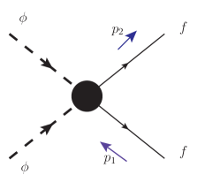
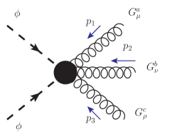
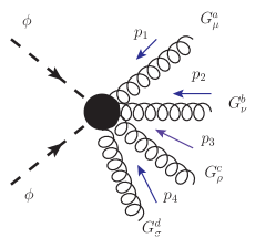
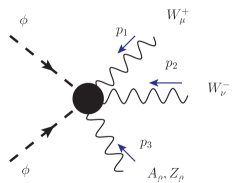
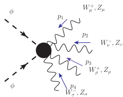
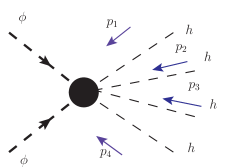
Figure 2: Effective processes contributing to relic density of dark matter. Here $2\rightarrow 3$ and $2\rightarrow 4$ processes are suppressed.

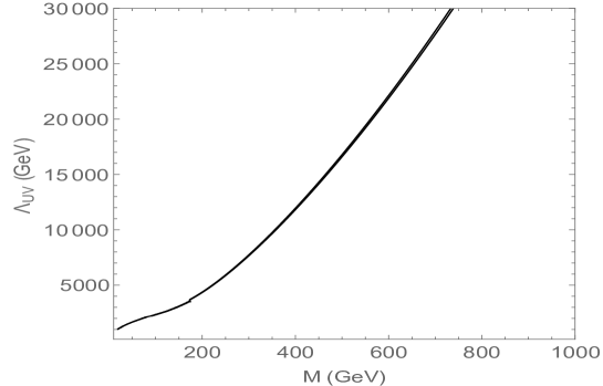
Figure 3: Allowed parameter space for the DM candidate. The kink in the graph at $M=m_{t}$ shows that beyond this mass, annihilation channels to top pairs are allowed.

4.2.1 Light Dark Matter

In this subsection we consider that the dark matter candidate is a dilaton, with a mass less than $350~{}{\rm GeV}$. The main annihilation channels will be $DM~{}DM\rightarrow f~{}\bar{f}$ where $f=t,b,\tau$, and $DM~{}DM\rightarrow gg,\gamma\gamma,W^{+}W^{-},ZZ$ . Hence the total thermally averaged cross section for LDM can be written as:

$$\langle\sigma v\rangle_{LDM}=\langle\sigma v\rangle_{G_{\mu}G^{\mu}}+\langle\sigma v\rangle_{A_{\mu}A^{\mu}}+\langle\sigma v\rangle_{W_{\mu}W^{\mu}}+\langle\sigma v\rangle_{Z_{\mu}Z^{\mu}}+\langle\sigma v\rangle_{hh}+\sum_{f}\langle\sigma v\rangle_{ff}$$ (41)

In fig. (4(a)) , we show the allowed annihilation channels of LDM candidate into SM particles.

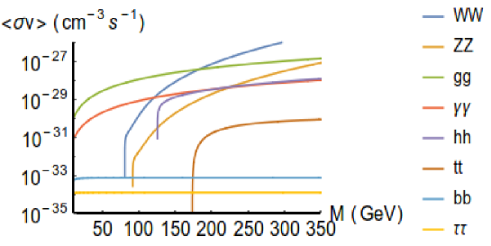
(a) $\langle\sigma v\rangle$ for LDM

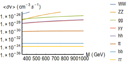
(b) $\langle\sigma v\rangle$ for HDM

Figure 4: Top panel:Figure showing annihilation cross-sections of LDM to SM particles. Bottom panel: Figure showing annihilation cross-sections of HDM to SM particles.

4.2.2 Heavy Dark Matter

In this subsection we consider that the Dark Matter has a mass greater $350~{}{\rm GeV}$. The annihilation channels remain the same, however as we can see from fig.(3), the corresponding scale of the EFT increases by an order of magnitude. We also show the same annihilation channels as the LDM in fig. (4(b)). We observe similar features as observed in the previous case. However, the annihilation cross-sections are well below the current experimental sensitivity, and cannot be probed by present experiments. This extra suppression is mainly due to larger scales (by a factor of $10$) and universal ${O(1)}$ coupling.

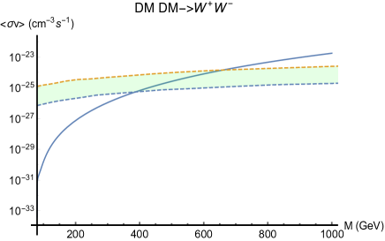
Figure 5: Comparison of DM annihilation channel with bounds given by FermiLAT.

To show that these are well within the bounds given by FermiLAT  Ackermann:2015zua , we show one specific case of DM annihilating into $W$ bosons in fig. (5) . The green shaded region shows $2\sigma$ bounds on the thermally averaged cross section for the process. We find that for most of our parameter space, the predictions of our model are well within these bounds.

5 Constraints from dark matter self interaction

In this subsection we will explicitly discuss about the constraints on the parameters of the background models of extended theories of gravity- (1) local $f(R)$ gravity and (2) non-minimally coupled dilaton with gravity, by applying the constraints from dark matter self interaction. To describe this fact let us consider the process $\phi\phi\rightarrow\phi\phi$, where $\phi$ is the scalar dark matter candidate in Einstein frame as introduced earlier by applying conformal transformation in the metric. Here $\phi\phi\rightarrow\phi\phi$ represents dark matter self-interaction and characterized by the coefficient of $\phi^{4}$ term in the effective potential in Einstein frame i.e. estimated by the term $V^{{}^{\prime\prime\prime\prime}}_{0}/4!$.

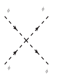
Figure 6: DM-DM self interaction at the tree level

The simplest four point contact interaction diagram contributing at the tree level is depicted in fig. 6. In this case the S-matrix element and amplitude of the $\phi\phi\rightarrow\phi\phi$ process is given by:

$$i{\cal M}_{\phi\phi\rightarrow\phi\phi} = -i\lambda=-iV^{{}^{\prime\prime\prime\prime}}_{0}/4!,$$ (42)

$$|{\cal M}_{\phi\phi\rightarrow\phi\phi}|^{2} = \lambda^{2}=\left(V^{{}^{\prime\prime\prime\prime}}_{0}/4!\right)^{2}.$$ (43)

Consequently the differential scattering cross section for the $\phi\phi\rightarrow\phi\phi$ process is given by:

$$\frac{d\sigma}{d\Omega} = \frac{|{\cal M}_{\phi\phi\rightarrow\phi\phi}|^{2}}{64\pi^{2}s}=\frac{\lambda^{2}}{64\pi^{2}s}=\frac{\left(V^{{}^{\prime\prime\prime\prime}}_{0}/4!\right)^{2}}{64\pi^{2}s},$$ (44)

where $s$ is the Mandelstum variable and in centre of mass frame characterized by $p_{1,2}=(M,0,0,\pm v)$ it is given by:

$$s = (p_{1}+p_{2})^{2}=4M^{2},$$ (45)

where $p_{1,2}$ are the momenta of the two incoming scalar dark matter particle, $M$ is the mass of the scalar dark matter. Finally using Eq (45) and integrating over the total solid angle one can finally write down the expression for the scattering cross section for the $\phi\phi\rightarrow\phi\phi$ self interaction process as:

$$\sigma = \frac{|{\cal M}_{\phi\phi\rightarrow\phi\phi}|^{2}}{64\pi M^{2}}=\frac{\lambda^{2}}{64\pi M^{2}}=\frac{\left(V^{{}^{\prime\prime\prime\prime}}_{0}/4!\right)^{2}}{64\pi M^{2}}.$$ (46)

Now, in order to have an observable effect on dark matter halos over large(cosmological) timescales, we have to satisfy the following constraint in the present context Kaplinghat:2013kqa :

$$\frac{\sigma}{M}\lesssim 1~{}{\rm cm}^{2}/g=5\times 10^{3}~{}{\rm{\rm GeV}}^{-3}.$$ (47)

Further using Eq (46) in Eq (47), we get the following simplified expression for this constraint:

$$\frac{\lambda^{2}}{64\pi M^{3}} \lesssim 5\times 10^{3}~{}{\rm{\rm GeV}}^{-3},$$

$$\Rightarrow\frac{\left(V^{{}^{\prime\prime\prime\prime}}_{0}/4!\right)^{2}}{64\pi M^{3}} \lesssim 5\times 10^{3}~{}{\rm{\rm GeV}}^{-3}.$$ (48)

Further depending on the different types of models of modified gravity theory as discussed in this paper, we will get a different value of the self-interaction parameter $\lambda$ , which is a function of some other parameters characterising the types of modified gravity. In our discussion for $f(R)$ gravity these parameters are $a$, $b$ and $n$, for non-minimally coupled dilaton with gravity and SM it is characterised by the non-minimal coupling parameter $\xi$ as introduced earlier.

5.1 Case I: For $f(R)$ gravity

A. For $n=2$:
In this case $f(R)$ is fiven by:

$$f(R)=aR+bR^{2},$$ (49)

where we set $a=1$ to have consistency with the Einstein gravity at the leading order and in this case $b$ is the only parameter that has to be constrained from dark matter self interaction . Additionally it is important to note that the mass dimension of $b$ for $n=2$ case is $-2$.

In this case the self-interaction parameter $\lambda$ or $V^{{}^{\prime\prime\prime\prime}}_{0}/4!$ can be expressed as:

$$\lambda = V^{{}^{\prime\prime\prime\prime}}_{0}/4!={\cal M}_{\phi\phi\rightarrow\phi\phi}=\frac{14}{9b\Lambda^{2}_{UV}},$$ (50)

where $\Lambda_{UV}$ is the UV cut-off of the effective field theory and further using Eq (50) the constraint condition stated in Eq (5) can be recast as:

$$|b| \gtrsim \frac{7}{1800\sqrt{2\pi}\Lambda^{2}_{UV}}\times\left(\frac{\rm{\rm GeV}}{M}\right)^{3/2}$$ (51)

$$= \left\{\begin{array}[]{ll}\displaystyle 3.87\times 10^{-13}~{}{\rm{\rm GeV}}^{-2}&\mbox{\small{\bf for ~{}LDM~{}with~{}$M=100~{}{\rm{\rm GeV}},~{}\Lambda_{UV}=2000~{}{\rm{\rm GeV}}$}}\\ \displaystyle 3.46\times 10^{-16}~{}{\rm{\rm GeV}}^{-2}&\mbox{\small{\bf for ~{}HDM~{}with~{}$M=500~{}{\rm{\rm GeV}},~{}\Lambda_{UV}=20000~{}{\rm{\rm GeV}}$}}.\end{array}\right.$$ (54)

Thereby, depending on the choice of the dark matter mass $M$ and UV cut-off $\Lambda_{UV}$ parameters, we can constrain the parameter $b$ from dark matter self-interaction.
B. For $n>2$:
In this case $f(R)$ is fiven by:

$$f(R)=aR+bR^{n},~{}~{}~{}~{}~{}{\bf with~{}}n>2$$ (55)

where for physical consistency, we set $a\neq 1$ and in this case, $a$ and $b$ are the parameters to be constrained from dark matter self interaction for $n>2$ case. Here it is important to note that, for the further numerical estimation we set $n=3$. Additionally it is important to note that the mass dimension of $b$ for $n=3$ case is $-4$.

In this case the self-interaction parameter $\lambda$ can be expressed as:

$$\lambda = V^{{}^{\prime\prime\prime\prime}}_{0}/4!={\cal M}_{\phi\phi\rightarrow\phi\phi},$$ (56)

where $\Lambda_{UV}$ is the UV cut-off of the effective field theory. Calculations give

$$\lambda=\frac{0.0004+a\left[-0.0552+a\left(0.2405+(0.1140a-0.2958)a\right)\right]}{(1-a)^{2.5}b^{0.5}\Lambda^{2}_{UV}}$$

The allowed values of the parameters $a$ and $b$ for $n=3$ is shown in fig. 7(a). This figure is shown for $M=100~{}{\rm{\rm GeV}}$ and $\Lambda_{UV}=2~{}{\rm TeV}$. The plot for the HDM candidate ($M=500~{}{\rm{\rm GeV}}$ and $\Lambda_{UV}=20~{}{\rm TeV}$) look exactly the same. We observe that as $a$ approaches 1, the value of $b$ rises asymptotically and grows, whereas, for values of $a>1$, $b$ is negative and starts becoming smaller. We have checked that the nature of the results are similar for $n=4$ also, although the allowed values of $a$ and $b$ are slightly different.

5.2 Case II: For non-minimally coupled gravity

Here we will discuss the situation where $\xi\neq 1/6,\frac{\phi}{\Lambda_{UV}}>>\frac{1}{\xi}$ and the effect of the non-minimal coupling $\xi$ can be visualized prominently as it couples to the SM sector. The other case, $\xi\neq 1/6,\frac{\phi}{\Lambda_{UV}}<<\frac{1}{\xi}$, is not relevant in the present context as in this case the effect of the non-minimal coupling $\xi$ can be neglected and SM sector couples to gravity minimally. In $\xi\neq 1/6,\frac{\phi}{\Lambda_{UV}}>>\frac{1}{\xi}$ case, the only parameter for the modified gravity theory is the non-minimal coupling $\xi$ for the given value of dimensionless coefficients $C_{0}(g),C_{2}(g)$ and $C_{4}(g)$ .Here we will constrain $\xi$ using the constraint from dark matter self interaction. For the sake of simplicity we set $C_{0}(g)\sim C_{2}(g)\sim C_{4}(g)\sim{\cal O}(1)$.

In $\xi\neq 1/6,\frac{\phi}{\Lambda_{UV}}>>\frac{1}{\xi}$ the self-interaction parameter $\lambda$ can be expressed as:

$$\lambda = V^{{}^{\prime\prime\prime\prime}}_{0}/4!={\cal M}_{\phi\phi\rightarrow\phi\phi}=\frac{14+\xi(16\xi-15)}{1944\xi^{2}},$$ (57)

where $\Lambda_{UV}$ is the UV cut-off the effective field theory.

In this case, we show a plot of the parameter $\xi$ as a function of $M$ in fig. 7(b). We find that for a larger mass of the scalaron, a smaller value of $\xi\sim{\cal O}(10^{-5})$ is favored. The range of $M$ is taken so as to cover the entire parameter space for LDM and HDM candidates.

Thus, we observe that interpreting the dilaton as a dark matter candidate naturally incorporates dark matter self interaction and this can be directly used to put bounds on the parameters of the extended theories of gravity. We have presented a tree level analysis of the self interactions. This will receive corrections from higher order processes which have not been considered here.

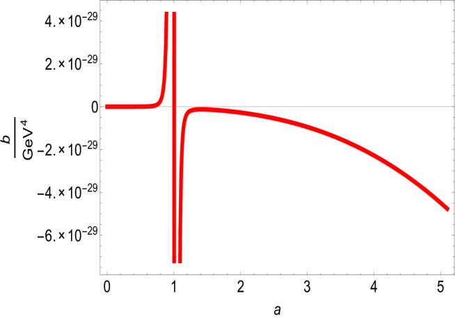
(a) $f(R)$ gravity, $n=3$

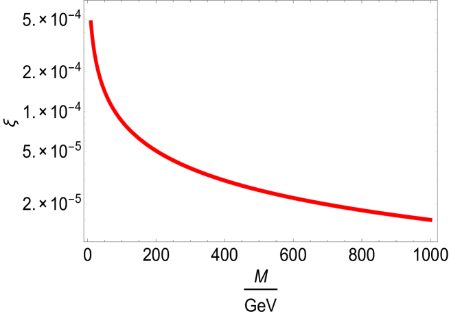
(b) Non Minimally Coupled Gravity

Figure 7: Plots showing variation of the parameters of modified gravity. In fig. 7(a), we show a variation of the parameters $a$ and $b$ in $f(R)=aR+bR^{n}$ for $n=3$. Notice the non-analytic behaviour at $a=1$. This graph is plotted for $M=100~{}{\rm{\rm GeV}}$ and $\Lambda_{UV}=2~{}{\rm TeV}$. The plots look exactly the same for the HDM candidate also.
In fig. 7(b), we show a plot of the parameter $\xi$ of the non-minimally coupled gravity as a function of DM mass.

6 Alternate UV completion of the Effective Field Theory

In this section, we plan to highlight some of the well known models which behave similarly as the effective field theory in the present context. Matter gravity interaction after a conformal transformation, generates terms involving interactions of the DM with other SM particles through the Lagrangian density,

$$\mathcal{L}_{int}=\frac{\phi^{2}}{\Lambda_{UV}^{2}}\mathcal{L}_{SM},$$ (58)

where $\Lambda_{UV}$ is the mass scale of the effective theory, below which this effective description works well.

The usual procedure is to start with description of a UV complete theory. If the UV complete theory contains a heavy particle of mass ${\cal M}\sim\Lambda_{UV}$, we integrate out that particle to get an effective Wilsonian operator at energies less than the UV cut-off scale $\Lambda_{UV}$, which contains all other particles with masses lighter than $\Lambda_{UV}$. To compare one UV complete model with the framework of effective description in the present context, we have to investigate if all the DM interaction operators are generated in that model.

In order to quantify the validity of the effective field theory, we can compare its cross section with that from full theory at momentum transfer $Q_{tr}$ in the process,

$$pp\rightarrow\phi\phi+jet/\gamma,$$ (59)

where $\phi$ is the scalar dark matter candidate in the model. The cross sections are calculated for $Q_{tr}<\Lambda_{UV}$, with $\Lambda_{UV}$ being the scale of the corresponding theory Busoni:2013lha ; Busoni:2014sya ; Busoni:2014haa . For the effective theory the scale can be taken arbitrarily but measurement of observables puts constraints on it. On the other hand, scale of a complete theory depends on particle to be integrated out from the theory.

6.1 Inert Higgs Doublet Model for low $\Lambda_{UV}$

Inert Higgs doublet model (IHDM) is a complete description where there is a DM candidate which can have interaction operators similar to the effective f(R) theory, at some particular mass scale. There are many studies in literature which look at the DM aspect of IHDM. A recent studyDiaz:2015pyv has treated the non-SM CP even scalar in the IHDM as the DM candidate and found out allowed parameter space satisfying the relic density. Part of this parameter space gets ruled out from the direct detection and collider physics constraints. An earlier study LopezHonorez:2006gr analyses the DM relic abundance and prospects for direct or indirect detection in detail. Refs.LopezHonorez:2010tb ; Honorez:2010re discuss about new updated parameter regions in the IHDM. Ref.Gustafsson:2007pc provides explanation of presence of $\gamma~{}$lines in the IHDM.

The Inert Higgs Doublet model is the minimal and simplest extension of the SM as it contains one extra scalar SU(2) doublet $\Phi_{2}$, apart from the SM-Higgs doublet $\Phi_{1}$ whose neutral component takes vacuum expectation value (vev) equal to v. It also couples to SM quarks and SM leptons similar to the SM-Higgs. $\Phi_{2}$ does not get any vev. It also does not couple to SM quarks and leptons. We also additionally enforce a $Z_{2}$ symmetry which transforms

$$\Phi_{1} \rightarrow \Phi_{1},$$ (60)

$$\Phi_{2} \rightarrow -\Phi_{2},$$ (61)

and other SM fields remain invariant under it. Most general CP-invariant, $Z_{2}$ symmetry abiding scalar potential is given as:

$$V(\Phi_{1},\Phi_{2})=\mu_{1}^{2}|\Phi_{1}|^{2}+\mu_{2}^{2}|\Phi_{2}|^{2}+\lambda_{1}|\Phi_{1}|^{4}+\lambda_{2}|\Phi_{2}|^{4}+\lambda_{3}|\Phi_{1}|^{2}|\Phi_{2}|^{2}$$

$$+\lambda_{4}|\Phi_{1}^{\dagger}\Phi_{2}|^{2}+\frac{\lambda_{5}}{2}((\Phi_{1}^{\dagger}\Phi_{2})^{2}+h.c.),$$ (62)

where $\mu_{i}^{2},\lambda_{i}~{}$s are taken real. We define two scalar doublets in the unitary gauge as:

$$\Phi_{1}=\begin{pmatrix}0\\ \frac{(v+h)}{\sqrt{2}}\end{pmatrix}\ ;\qquad\Phi_{2}=\begin{pmatrix}H^{+}\\ \frac{(S+iA)}{\sqrt{2}}\end{pmatrix}.$$ (63)

With these definitions we get the mass terms and the interaction Lagrangian of the scalar sector:

$$\mathcal{L}\supset\frac{1}{2}m_{h}^{2}h^{2}+\frac{1}{2}m_{S}^{2}S^{2}+\frac{\lambda}{2}vhSS+\frac{\lambda}{4}h^{2}S^{2}+\frac{\lambda_{2}}{2}S^{2}A^{2}+\text{other interactions},$$ (64)

where

$$m_{h}^{2}=2\lambda_{1}v^{2},m_{S}^{2}=\mu_{2}^{2}+\frac{\lambda}{2}v^{2}\ \ \text{with}\ \ \\ \lambda=\lambda_{3}+\lambda_{4}+\lambda_{5},$$ (65)

and A is the CP-odd scalar of the model. Yukawa coupling in this theory is written as

$$\mathcal{L}_{yuk}=y_{q}\bar{Q}_{L}\Phi_{1}q_{R}+h.c.,$$ (66)

which gives the mass of the fermions and also the $h\bar{q}q$ couplings. Due to the $Z_{2}$ symmetry imposed here, S can not decay to fermion channels. The $m_{S}$ can be made sufficiently small avoiding its decay to other scalars and WW/ZZ modes. Therefore we take $S$ as the DM candidate having direct interactions with the Higgs. This Lagrangian can give us processes like

$$pp\rightarrow SS+jet/\gamma$$ (67)

directly by a Higgs mediated process as shown in fig. 8. At $\Lambda_{UV}<m_{h}$, we can integrate out the Higgs boson to get effective vertex $~{}\bar{q}qSS$, which is the kind of effective coupling to produce DM in the f(R) theory. If we take S as the dilation then $f(R)$ theory in first order generates a coupling $\frac{m_{q}}{\Lambda_{UV}^{2}}\bar{q}qSS$. In DM DM annihilation, processes with two final state particles contribute dominantly. We consider here the effective operators that only contribute to DM annihilation with two body final state. At $\Lambda_{UV}\sim m_{h}$ theory contains the DM candidate, W, Z boson and all SM fermions except the top quark. In IHDM heavy Higgs (h) has all SM like couplings i.e. standard Yukawa and hWW and hZZ couplings. Combining those with the hSS coupling present in the model we get effective operators of the form $\bar{q}qSS$, $WWSS$ and $ZZSS$ integrating out the Higgs. The couplings $h\gamma\gamma,hgg$ are present in the 1-loop level. So operators like $SS\gamma\gamma,SSgg$ also gets generated as the effective form of IHDM at $\Lambda_{UV}\sim m_{h}$. So we can generate all operators of $f(R)$ theory involving DM annihilation from the inert Higgs doublet model. We can check the validity of the effective theory description of $f(R)$ gravity comparing it with the inert 2HDM contributions to some process involving DM.

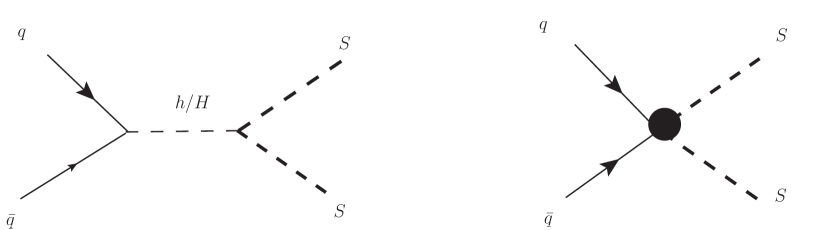
Figure 8: Left:$~{}q\bar{q}\rightarrow~{}SS$ in the full theory. Right: Effective process, after integrating out the heavy mediator.

6.2 UV complete model for high $\Lambda_{UV}$

We construct a model where we do not directly add effective operators contributing to DM pair production and DM annihilation processes as described above. We introduce a heavy scalar H as a part of third scalar doublet introduced in the IHDM. Here this new doublet acquires a non zero vev $v_{H}$, resulting in a non zero HAA/HSS vertex which originates from quartic coupling. Similarly H also couples to SM fermions and gauge bosons similarly as SM Higgs, though with different couplings. The Lagrangian consisting of H interaction terms is given as,

$$L\supset\frac{1}{2}m_{H}^{2}H^{2}+\lambda_{H}HSS+y^{H}_{q}H\bar{q}q+g^{H}_{V}HVV+..,$$ (68)

where $V=\left\{W,Z\right\}$ and $q$ denotes any SM fermion. At $\Lambda_{UV}\sim m_{H}$, heavy scalar H gets integrated out from our model to provide effective operators like $\bar{q}qSS,VVSS$, which are similar to the operators present in the effective f(R) theory. So with big $\Lambda_{UV}$ we can calculate DM cross sections.

7 Conclusion

To summarize, in the present article, we have addressed the following points:

• In this paper, we have proposed background models of extended theories of gravity, which are minimally coupled to SM fields. Initially we have started with a model where the usual Einstein gravity is minimally coupled with the SM sector. But to explain the genesis of dark matter without affecting the SM particle sector, we have further modified the gravity sector by allowing quantum corrections motivated from (1) local $f(R)$ gravity and (2) non-minimally coupled dilaton with gravity and SM sector.

• Next we have constructed an effective theory in the Einstein frame by applying conformal transformation on the metric. We have explicitly discussed the rules and detailed techniques of conformal transformation in the gravity sector as well as in the matter sector. Here for completeness, we have also presented the results for arbitrary $D$ space-time dimensions. We have used $D=4$ in the rest of our analysis.

• Then we have also shown that the effective theory constructed from (1) local $f(R)$ gravity and (2) non-minimally coupled dilaton with gravity and SM sector looks exactly same.

• Here we have used the relic constraint as observed by Planck 2015 to constrain the scale of the effective field theory $\Lambda_{UV}$ as well as the dark matter mass $M$. We have considered two cases- (1) light dark matter (LDM) and (2) heavy dark matter (HDM), and deduced upper bounds on the thermally averaged cross section of dark matter annihilating to SM particles, in the non-relativistic limit.

• We have modelled self-interactions of dark matter from their effective potentials in both cases-(1) local $f(R)$ gravity and (2) non-minimally coupled dilaton with gravity and SM sector. Using the present constraint on dark matter self interactions, we have constrained the parameters of these two gravity models.

• Next we have proposed different UV complete models from a particle physics point of view, which can give rise to the same effective theory that we have deduced from extended theories of gravity. We have mainly considered two models- (1) Inert Higgs Doublet model for LDM and (2) Inert Higgs Doublet model with a new heavy scalar for HDM. We have also explicitly shown that the UV completion of this effective field theory need not come from modifications to the matter sector, but rather from extensions of the gravity sector.

• To conclude, we note that dark matter can indeed be considered to be an artifact of extended theories of gravity. In our work, we have presented a dark matter candidate which is generated purely from the gravity sector. We have presented bounds on the mass of such a DM candidate, depending on the scale of the effective theory considered.

The future prospects of this work are given below:

• The prescribed ideas can be worked out to derive cosmological constraints for other modified gravity frameworks i.e. Randall Sundrum single braneworld (RSII) Randall:1999vf ; Maartens:2010ar ; Brax:2004xh ; Shiromizu:1999wj ; Choudhury:2014sua ; Choudhury:2011sq ; Choudhury:2011rz ; Choudhury:2012ib ; Choudhury:2015jaa   ,Einstein-Hilbert-Gauss-Bonnet (EHGB) gravity Choudhury:2013eoa ; Choudhury:2012yh ; Choudhury:2015yna ; Choudhury:2013dia , Dvali-Gabadadze-Porrati (DGP) braneworld Dvali:2000hr and Einstein-Gauss-Bonnet-Dilaton (EGBD) gravity Choudhury:2013yg ; Choudhury:2013aqa ; Choudhury:2014hna ; Choudhury:2015wfa ; Choudhury:2016wlj etc.

• Using the observational constraints from indirect detection of dark matter one can further constrain various classes of modified theories of gravity scenario.

• Detailed study of DM collider and direct detection constraints Duerr:2015aka on the effective theory prescription and the study of the effectiveness of the prescribed theory from the various extended theories of gravity is one of the promising areas of research.

• Explaining the genesis of dark matter in presence of non-standard/ non-canonical kinetic term Choudhury:2015hvr and also exploring the highly non-linear regime of effective field theory are open issues in this literature.

• The relation between dark matter abundance, primordial magnetic field and gravity waves and leptogenesis scenario from these effective operators can be studied. In the case of RSII single membrane, some of the issues have been recently worked out in ref. Choudhury:2015eua .

• The exact role of dark matter in the case of alternatives to inflation - specifically for cyclic and bouncing cosmology Choudhury:2015baa ; Choudhury:2015fzb ; Choudhury:2015fzb can also be studied in the present context.

8 Appendix A: Conformal transformations in extended theories of gravity

8.1 Conformal transformations in gravity sector

Consider a $D$ dimensional space-time, where ${\cal M}$ is a smooth manifold and $g_{\mu\nu}$ is the Lorentzian metric on it. Under conformal transformation the metric $g_{\mu\nu}$, its inverse $g^{\mu\nu}$, determinant $\sqrt{-g}$ and the infinitesimal line element transform as birell:

$$g_{\mu\nu}\Longrightarrow\tilde{g}_{\mu\nu} = \Omega^{2}(x)g_{\mu\nu},$$ (69)

$$g^{\mu\nu}\Longrightarrow\tilde{g}^{\mu\nu} = \Omega^{-2}(x)g^{\mu\nu},$$ (70)

$$g_{\mu\nu}g^{\nu\beta}=\delta_{\mu}^{\beta}\Longrightarrow\tilde{g}_{\mu\nu}\tilde{g}^{\nu\beta} = \Omega^{2}(x)g_{\mu\nu}\Omega^{-2}(x)g^{\nu\beta}=\delta_{\mu}^{\beta},$$ (71)

$$\sqrt{-g}\Longrightarrow\sqrt{-\tilde{g}} = \Omega^{D}(x)\sqrt{-g},$$ (72)

$$ds^{2}=g_{\mu\nu}dx^{\mu}dx^{\nu}\Longrightarrow d\tilde{s}^{2} = \tilde{g}_{\mu\nu}d\tilde{x}^{\mu}d\tilde{x}^{\nu}=\Omega^{2}(x)g_{\mu\nu}dx^{\mu}dx^{\nu}=\Omega^{2}(x)ds^{2}$$ (73)

where the conformal factor $\Omega(x)$ is a smooth, non-vanishing, spacetime point dependent rescaling of the metric. The conformal transformations can shrink or stretch the distances between the two points described by the same coordinate system $x^{\mu}$ (where $\mu=0,1,2,\cdots,D$) on the manifold ${\cal M}$. However, these transformations preserve the angles between vectors, particularly null vectors, which define light cones, thereby leading to a conservation of the global causal structure of the manifold. For simplicity, if we take the conformal factor to be a constant space-time independent function, then it is known as a scale transformation. On the contrary, any arbitrary $D$ dimensional coordinate transformations $x^{\mu}\rightarrow\tilde{x}^{\mu}$ only change the structural form of the coordinates, but not the associated geometry. This implies that coordinate transformations are completely different from conformal transformations, which connect two different frames via conformal couplings.

Finally, the Einstein tensor transforms as:

$$G_{\mu\nu}\Longrightarrow\tilde{G}_{\mu\nu} = G_{\mu\nu}+\left(\frac{D-2}{2}\right)\Omega^{-2}(x)\left[4\partial_{\mu}\Omega(x)\partial_{\nu}\Omega(x)+(D-5)\partial_{\alpha}\Omega(x)\partial^{\alpha}\Omega(x)g_{\mu\nu}\right]$$ (74)

$$~{}~{}~{}~{}~{}~{}~{}~{}~{}~{}~{}~{}~{}~{}~{}~{}-(D-2)\Omega^{-1}(x)\left[\triangledown_{\mu}\triangledown_{\nu}-g_{\mu\nu}\Box\right]\Omega(x),$$

$$\tilde{G}_{\mu\nu}\Longrightarrow{G}_{\mu\nu} = \tilde{G}_{\mu\nu}+\left(\frac{D-2}{2}\right)\Omega^{-2}(x)(D-1)\partial_{\alpha}\Omega(x)\partial^{\alpha}\Omega(x)\tilde{g}_{\mu\nu}$$ (75)

$$~{}~{}~{}~{}~{}~{}~{}~{}~{}~{}~{}~{}~{}~{}~{}~{}+(D-2)\Omega^{-1}(x)\left[\tilde{\triangledown}_{\mu}\tilde{\triangledown}_{\nu}-\tilde{g}_{\mu\nu}\widetilde{\Box}\right]\Omega(x).$$

We observe that, conformal transformations under some specific conditions behave like duality transformation in superstring theory. To demonstrate this, let us define the conformal factor as:

$$\Omega(x)=e^{\omega(x)}=e^{\frac{\kappa}{\sqrt{6}}\phi(x)},$$ (76)

where $\omega(x)=\frac{\kappa}{\sqrt{6}}\phi(x)$ represents the new scalar field “scalaron” or “dilaton”. Here we define $\kappa=\Lambda^{-1}_{UV}$. Now, the conformal transformation in the metric $g_{\mu\nu}$, its inverse $g^{\mu\nu}$, determinant $\sqrt{-g}$ and consequently the infinitesimal line element transform as:

$$g_{\mu\nu}\Longrightarrow\tilde{g}_{\mu\nu} = e^{2\omega(x)}g_{\mu\nu}=e^{\frac{2\kappa}{\sqrt{6}}\phi(x)}g_{\mu\nu},$$ (77)

$$g^{\mu\nu}\Longrightarrow\tilde{g}^{\mu\nu} = e^{-2\omega(x)}g^{\mu\nu}=e^{-\frac{2\kappa}{\sqrt{6}}\phi(x)}g_{\mu\nu},$$ (78)

$$g_{\mu\nu}g^{\nu\beta}=\delta_{\mu}^{\beta}\Longrightarrow\tilde{g}_{\mu\nu}\tilde{g}^{\nu\beta} = e^{2\omega(x)}g_{\mu\nu}e^{-2\omega(x)}g^{\nu\beta}=\delta_{\mu}^{\beta},$$ (79)

$$\sqrt{-g}\Longrightarrow\sqrt{-\tilde{g}} = e^{D\omega(x)}\sqrt{-g}=e^{\frac{D\kappa}{\sqrt{6}}\phi(x)}\sqrt{-g},$$ (80)

$$ds^{2}=g_{\mu\nu}dx^{\mu}dx^{\nu}\Longrightarrow d\tilde{s}^{2} = \tilde{g}_{\mu\nu}d\tilde{x}^{\mu}d\tilde{x}^{\nu}=e^{2\omega(x)}g_{\mu\nu}dx^{\mu}dx^{\nu}=e^{\frac{2\kappa}{\sqrt{6}}\phi(x)}ds^{2}.$$ (81)

In the present context, the Einstein frame and the Jordan frame are connected via the following duality transformation:

$$\Omega(x)=e^{\omega(x)}=e^{\frac{\kappa}{\sqrt{6}}\phi(x)}\Longleftrightarrow\Omega^{-1}(x)=e^{-\omega(x)}=e^{-\frac{\kappa}{\sqrt{6}}\phi(x)},$$ (82)

which is exactly same as the weak-strong coupling duality in superstring theory. Using Eq (76) we get:

$$\Omega^{-1}(x)\partial_{\mu}\Omega(x) = \partial_{\mu}\omega(x)=\frac{\kappa}{\sqrt{6}}\partial_{\mu}\phi(x),$$ (83)

$$\Omega^{-1}(x)\triangledown_{\mu}\triangledown_{\nu}\Omega(x) = \triangledown_{\mu}\triangledown_{\nu}\omega(x)+\partial_{\mu}\omega(x)\partial_{\nu}\omega(x)=\frac{\kappa}{\sqrt{6}}\triangledown_{\mu}\triangledown_{\nu}\phi(x)+\frac{\kappa^{2}}{6}\partial_{\mu}\phi(x)\partial_{\nu}\phi(x),~{}~{}~{}~{}~{}~{}~{}~{}~{}~{}~{}~{}~{}~{}$$ (84)

$$\Omega^{-1}(x)\Box\Omega(x) = \Box\omega(x)+\partial_{\mu}\omega(x)\partial_{\nu}\omega(x)=\frac{\kappa}{\sqrt{6}}\Box\phi(x)+\frac{\kappa^{2}}{6}\partial_{\mu}\phi(x)\partial_{\nu}\phi(x).~{}~{}~{}~{}~{}~{}$$ (85)

Consequently in terms of “scalaron” or “dilaton”, the Christoffel connections can be recast as:

$$\Gamma^{\beta}_{\mu\nu}\Longrightarrow\tilde{\Gamma}^{\beta}_{\mu\nu} = \Gamma^{\beta}_{\mu\nu}+\left[\delta^{\beta}_{\mu}\partial_{\nu}+\delta^{\beta}_{\nu}\partial_{\mu}-g_{\mu\nu}g^{\beta\alpha}\partial_{\alpha}\right]\omega(x)$$ (86)

$$= \Gamma^{\beta}_{\mu\nu}+\frac{\kappa}{\sqrt{6}}\left[\delta^{\beta}_{\mu}\partial_{\nu}+\delta^{\beta}_{\nu}\partial_{\mu}-g_{\mu\nu}g^{\beta\alpha}\partial_{\alpha}\right]\phi(x),$$

$$\Gamma^{\nu}_{\mu\nu}\Longrightarrow\tilde{\Gamma}^{\nu}_{\mu\nu} = \Gamma^{\nu}_{\mu\nu}+D\partial_{\mu}\omega(x)=\Gamma^{\nu}_{\mu\nu}+\frac{\kappa D}{\sqrt{6}}\partial_{\mu}\phi(x),$$ (87)

$$\tilde{\Gamma}^{\beta}_{\mu\nu}\Longrightarrow{\Gamma}^{\beta}_{\mu\nu} = \tilde{\Gamma}^{\beta}_{\mu\nu}-\left[\delta^{\beta}_{\mu}\partial_{\nu}+\delta^{\beta}_{\nu}\partial_{\mu}-\tilde{g}_{\mu\nu}\tilde{g}^{\beta\alpha}\partial_{\alpha}\right]\omega(x)$$ (88)

$$= \tilde{\Gamma}^{\beta}_{\mu\nu}-\frac{\kappa}{\sqrt{6}}\left[\delta^{\beta}_{\mu}\partial_{\nu}+\delta^{\beta}_{\nu}\partial_{\mu}-\tilde{g}_{\mu\nu}\tilde{g}^{\beta\alpha}\partial_{\alpha}\right]\phi(x),$$

$$\tilde{\Gamma}^{\nu}_{\mu\nu}\Longrightarrow{\Gamma}^{\nu}_{\mu\nu} = \tilde{\Gamma}^{\nu}_{\mu\nu}-D\partial_{\mu}\omega(x)=\tilde{\Gamma}^{\nu}_{\mu\nu}-\frac{\kappa D}{\sqrt{6}}\partial_{\mu}\phi(x).$$ (89)

Consequently, the Riemann tensors, Ricci tensors, and Ricci scalars can be expressed in terms of “scalaron” or “dilaton” as:

$$\tilde{R}^{\mu}_{\nu\alpha\beta}\Longrightarrow{R}^{\mu}_{\nu\alpha\beta} = \tilde{R}^{\mu}_{\nu\alpha\beta}-\left[\delta^{\mu}_{\beta}\tilde{\triangledown}_{\nu}\tilde{\triangledown}_{\alpha}-\delta^{\mu}_{\alpha}\tilde{\triangledown}_{\nu}\tilde{\triangledown}_{\beta}+\tilde{g}_{\nu\alpha}\tilde{\triangledown}^{\mu}\tilde{\triangledown}_{\beta}-\tilde{g}_{\nu\beta}\tilde{\triangledown}^{\mu}\tilde{\triangledown}_{\alpha}\right]\omega(x)$$ (90)

$$~{}~{}~{}+\left[\delta^{\mu}_{\alpha}\partial_{\nu}\omega(x)\partial_{\beta}\omega(x)-\delta^{\mu}_{\beta}\partial_{\nu}\omega(x)\partial_{\alpha}\omega(x)\right.$$

$$\left.~{}~{}~{}~{}+g_{\nu\beta}\partial^{\mu}\omega(x)\partial_{\alpha}\omega(x)-g_{\nu\alpha}\partial^{\mu}\omega(x)\partial_{\beta}\omega(x)\right]$$

$$~{}~{}~{}+\left[\delta^{\mu}_{\beta}\tilde{g}_{\nu\alpha}-\delta^{\mu}_{\alpha}\tilde{g}_{\nu\beta}\right]\tilde{g}_{\lambda\eta}\partial^{\lambda}\omega(x)\partial^{\eta}\omega(x)$$

$$= \tilde{R}^{\mu}_{\nu\alpha\beta}-\frac{\kappa}{\sqrt{6}}\left[\delta^{\mu}_{\beta}\tilde{\triangledown}_{\nu}\tilde{\triangledown}_{\alpha}-\delta^{\mu}_{\alpha}\tilde{\triangledown}_{\nu}\tilde{\triangledown}_{\beta}+\tilde{g}_{\nu\alpha}\tilde{\triangledown}^{\mu}\tilde{\triangledown}_{\beta}-\tilde{g}_{\nu\beta}\tilde{\triangledown}^{\mu}\tilde{\triangledown}_{\alpha}\right]\phi(x)$$

$$~{}~{}~{}+\frac{\kappa^{2}}{6}\left[\delta^{\mu}_{\alpha}\partial_{\nu}\phi(x)\partial_{\beta}\phi(x)-\delta^{\mu}_{\beta}\partial_{\nu}\phi(x)\partial_{\alpha}\phi(x)\right.$$

$$\left.~{}~{}~{}~{}+g_{\nu\beta}\partial^{\mu}\phi(x)\partial_{\alpha}\phi(x)-g_{\nu\alpha}\partial^{\mu}\phi(x)\partial_{\beta}\phi(x)\right]$$

$$~{}~{}~{}+\frac{\kappa^{2}}{6}\left[\delta^{\mu}_{\beta}\tilde{g}_{\nu\alpha}-\delta^{\mu}_{\alpha}\tilde{g}_{\nu\beta}\right]\tilde{g}_{\lambda\eta}\partial^{\lambda}\phi(x)\partial^{\eta}\phi(x).$$

$$\tilde{R}_{\mu\nu}\Longrightarrow{R}_{\mu\nu} = \tilde{R}_{\mu\nu}+(D-2)\left[\partial_{\mu}\omega(x)\partial_{\nu}\omega(x)-\tilde{g}_{\mu\nu}\partial_{\alpha}\omega(x)\partial^{\alpha}\omega(x)\right]$$ (91)

$$~{}~{}~{}+\left[(D-2)\tilde{\triangledown}_{\mu}\tilde{\triangledown}_{\nu}+\tilde{g}_{\mu\nu}\widetilde{\Box}\right]\omega(x)$$

$$= \tilde{R}_{\mu\nu}+\frac{\kappa^{2}(D-2)}{6}\left[\partial_{\mu}\phi(x)\partial_{\nu}\phi(x)-\tilde{g}_{\mu\nu}\partial_{\alpha}\phi(x)\partial^{\alpha}\phi(x)\right]$$

$$~{}~{}~{}+\frac{\kappa}{\sqrt{6}}\left[(D-2)\tilde{\triangledown}_{\mu}\tilde{\triangledown}_{\nu}+\tilde{g}_{\mu\nu}\widetilde{\Box}\right]\phi(x),$$

$$\tilde{R}\Longrightarrow{R} = e^{2\omega(x)}\left[\tilde{R}+2(D-1)\widetilde{\Box}\omega(x)\right.$$ (92)

$$\left.~{}~{}~{}~{}~{}~{}~{}~{}~{}~{}~{}~{}~{}-(D-2)(D-1)\partial_{\alpha}\omega(x)\partial_{\beta}\omega(x)\tilde{g}^{\alpha\beta}\right]$$

$$= e^{\frac{2\kappa}{\sqrt{6}}\phi(x)}\left[\tilde{R}+\frac{2\kappa(D-1)}{\sqrt{6}}\widetilde{\Box}\phi(x)\right.$$

$$\left.~{}~{}~{}~{}~{}~{}~{}~{}~{}~{}~{}~{}~{}-\frac{\kappa^{2}(D-2)(D-1)}{6}\partial_{\alpha}\phi(x)\partial_{\beta}\phi(x)\tilde{g}^{\alpha\beta}\right]$$

Additionaly, the d’Alembertial operator can be expressed in terms of “scalaron” or “dilaton” as:

$$\widetilde{\Box}\Longrightarrow{\Box} = e^{2\omega(x)}\left[\widetilde{\Box}-(D-2)\tilde{g}^{\mu\nu}\partial_{\mu}\omega(x)\partial_{\nu}\right]=e^{\frac{2\kappa}{\sqrt{6}}\phi(x)}\left[\widetilde{\Box}-\frac{\kappa(D-2)}{\sqrt{6}}\tilde{g}^{\mu\nu}\partial_{\mu}\phi(x)\partial_{\nu}\right].~{}~{}~{}~{}~{}~{}~{}~{}~{}$$ (93)

Finally, the Einstein tensor is transformed as:

$$\tilde{G}_{\mu\nu}\Longrightarrow{G}_{\mu\nu} = \tilde{G}_{\mu\nu}+\left(\frac{D-2}{2}\right)\left[\partial_{\mu}\omega(x)\partial_{\nu}\omega(x)+\left(\frac{D-3}{2}\right)\partial_{\alpha}\omega(x)\partial^{\alpha}\omega(x)\tilde{g}_{\mu\nu}\right]$$ (94)

$$~{}~{}~{}~{}~{}~{}~{}~{}~{}~{}~{}~{}~{}~{}~{}~{}+(D-2)\left[\tilde{\triangledown}_{\mu}\tilde{\triangledown}_{\nu}-\tilde{g}_{\mu\nu}\widetilde{\Box}\right]\omega(x)$$

$$= \tilde{G}_{\mu\nu}+\frac{\kappa^{2}}{6}\left(\frac{D-2}{2}\right)\left[\partial_{\mu}\phi(x)\partial_{\nu}\phi(x)+\left(\frac{D-3}{2}\right)\partial_{\alpha}\phi(x)\partial^{\alpha}\phi(x)\tilde{g}_{\mu\nu}\right]$$

$$~{}~{}~{}~{}~{}~{}~{}~{}~{}~{}~{}~{}~{}~{}~{}~{}+\frac{\kappa}{\sqrt{6}}(D-2)\left[\tilde{\triangledown}_{\mu}\tilde{\triangledown}_{\nu}-\tilde{g}_{\mu\nu}\widetilde{\Box}\right]\phi(x).$$

We use the results for $D=4$ to study the consequences in the context of dark matter.

8.2 Conformal transformations in matter sector

Let us assume that matter is minimally coupled with the gravity sector. In such a case, in an arbitrary $D$ dimensional space-time, the action can be written as:

$$S_{M}=\int d^{D}x\sqrt{-g}{\cal L}_{M},$$ (95)

which is invariant under the conformal transformation in the metric, as mentioned earlier. In our present context, in $D=4$, we have taken the matter sector to be SM i.e. ${\cal L}_{M}={\cal L}_{SM}$. Under this conformal transformation, the energy-momentum stress tensor transforms as:

$$\tilde{T}^{\mu\nu}_{M} = \frac{2}{\sqrt{-\tilde{g}}}\frac{\delta}{\delta\tilde{g}_{\mu\nu}}\left(\sqrt{-\tilde{g}}\tilde{\cal L}_{M}\right)=\Omega^{-D-2}(x){T}^{\mu\nu}_{M}=e^{-(D+2)w(x)}{T}^{\mu\nu}_{M}=e^{-\frac{\kappa}{\sqrt{6}}(D+2)\phi(x)}{T}^{\mu\nu}_{M},~{}~{}~{}~{}~{}~{}~{}~{}~{}~{}~{}~{}$$ (96)

$$\tilde{T}^{\mu}_{\nu,M} = \tilde{T}^{\mu\alpha}_{M}\tilde{g}_{\alpha\nu}=\Omega^{-D}(x){T}^{\mu}_{\nu,M}=e^{-Dw(x)}{T}^{\mu}_{\nu,M}=e^{-\frac{\kappa}{\sqrt{6}}D\phi(x)}{T}^{\mu}_{\nu,M},$$ (97)

$$\tilde{T}_{\mu\nu,M} = \tilde{T}^{\alpha\beta}_{M}\tilde{g}_{\alpha\mu}\tilde{g}_{\beta\nu}=\Omega^{-D+2}(x){T}_{\mu\nu,M}=e^{(2-D)w(x)}{T}_{\mu\nu,M}=e^{\frac{\kappa}{\sqrt{6}}(2-D)\phi(x)}{T}_{\mu\nu,M},$$ (98)

$$\tilde{T}_{M} = T^{\mu}_{\mu,M}=\Omega^{-D}(x){T}^{\mu}_{\mu,M}=e^{-Dw(x)}{T}^{\mu}_{\mu,M}=e^{-\frac{\kappa}{\sqrt{6}}D\phi(x)}{T}^{\mu}_{\mu,M},$$ (99)

where $\tilde{\cal L}_{M}$ is the energy-momentum stress tensor in Einstein frame and this is related to the Jordan frame via the following transformation rule:

$$\tilde{\cal L}_{M}=\Omega^{-D}(x){\cal L}_{M}=e^{-Dw(x)}{\cal L}_{M}=e^{-\frac{\kappa}{\sqrt{6}}D\phi(x)}{\cal L}_{M}.$$ (100)

Using the the fact that the matter sector is governed by a perfect fluid and the structural form of the conformal transformation in the metric, one can show that the density and pressure can be transformed in the Einstein frame as:

$$\tilde{\rho} = \Omega^{-D}(x)\rho=e^{-Dw(x)}\rho=e^{-\frac{\kappa}{\sqrt{6}}D\phi(x)}\rho,$$ (101)

$$\tilde{p} = \Omega^{-D}(x)p=e^{-Dw(x)}p=e^{-\frac{\kappa}{\sqrt{6}}D\phi(x)}p,$$ (102)

where $(\rho,p)$ and $(\tilde{\rho},\tilde{p})$ are the density and pressure of the matter content in Jordan and Einstein frame respectively. The results clearly show that if we impose conservation of the energy-momentum stress tensor in one frame then in the other conformally connected frame it is no longer conserved. Only if we assume that in both the frames matter content is governed by the traceless tensor, then conservation holds good in both the frames simultaneously. But for a general matter content this may not always be the case. For example, in the $D=4$ version of the Effective Field Theory discussed in this paper, we assume that the matter content is governed by the well known SM fields in the Jordan frame. But after applying the conformal transformation in the metric, the conformal coupling factor becomes

$$\Omega^{-4}(x)=e^{-4\omega(x)}=e^{-\frac{4\kappa}{\sqrt{6}}\phi(x)},$$ (103)

or more precisely, the “scalaron”or the “dilaton” field is interacting with the SM matter fields in the Einstein frame, which will act as the primary source of generating a scalar dark matter candidate from an extended theory of gravity.

9 Appendix B: Thermally averaged annihilation cross-section

Here we outline the annihilation cross section for the processes contributing to the relic density.

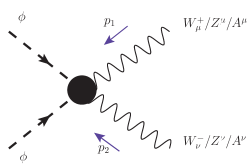
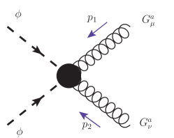
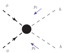
Figure 9: Effective processes contributing to relic density of dark matter.

$$\langle\sigma v\rangle_{NR_{G_{\mu}G^{\mu}}} = \frac{32M^{2}}{\pi\Lambda^{4}_{UV}}+\frac{16M^{2}}{\pi\Lambda^{4}_{UV}}v^{2}=a_{NR_{G_{\mu}G^{\mu}}}(\Lambda_{UV},M)+b_{NR_{G_{\mu}G^{\mu}}}(\Lambda_{UV},M)v^{2}~{}~{}~{}$$ (104)

$$\langle\sigma v\rangle_{NR_{W_{\mu}W^{\mu}}} = \frac{\sqrt{1-\frac{M_{W}^{2}}{M^{2}}}}{32\pi M^{2}}\left(\frac{64M^{4}}{\Lambda^{4}_{UV}}+\frac{64M^{8}}{\Lambda^{4}_{UV}M_{W}^{4}}-\frac{128M^{6}}{\Lambda^{4}_{UV}M_{W}^{2}}+\frac{8M_{W}^{4}}{\Lambda^{4}_{UV}}\right)$$ (105)

$$~{}~{}~{}~{}+\frac{\sqrt{1-\frac{M_{W}^{2}}{M^{2}}}}{32\pi M^{2}}\left(\frac{32M^{4}}{\Lambda^{4}_{UV}}+\frac{64M^{8}}{\Lambda^{4}_{UV}M_{W}^{4}}-\frac{96M^{6}}{\Lambda^{4}_{UV}M_{W}^{2}}\right)v^{2}$$

$$= a_{NR_{W_{\mu}W^{\mu}}}(\Lambda_{UV},M)+b_{NR_{W_{\mu}W^{\mu}}}(\Lambda_{UV},M)v^{2}$$

$$\langle\sigma v\rangle_{NR_{Z_{\mu}Z^{\mu}}} = \frac{\sqrt{1-\frac{M_{Z}^{2}}{M^{2}}}}{32\pi M^{2}}\sin^{4}\theta_{W}\left(\frac{64M^{4}}{\Lambda^{4}_{UV}}+\frac{64M^{8}}{\Lambda^{4}_{UV}M_{Z}^{4}}-\frac{128M^{6}}{\Lambda^{4}_{UV}M_{Z}^{2}}+\frac{8M_{Z}^{4}}{\Lambda^{4}_{UV}}\right)$$ (106)

$$~{}~{}~{}~{}+\frac{\sqrt{1-\frac{M_{Z}^{2}}{M^{2}}}}{32\pi M^{2}}\sin^{4}\theta_{W}\left(\frac{32M^{4}}{\Lambda^{4}_{UV}}+\frac{64M^{8}}{\Lambda^{4}_{UV}M_{Z}^{4}}-\frac{96M^{6}}{\Lambda^{4}_{UV}M_{Z}^{2}}\right)v^{2}$$

$$= a_{NR_{Z_{\mu}Z^{\mu}}}(\Lambda_{UV},M)+b_{NR_{Z_{\mu}Z^{\mu}}}(\Lambda_{UV},M)v^{2}$$

$$\langle\sigma v\rangle_{NR_{A_{\mu}A^{\mu}}} = \frac{4M^{2}\cos^{4}(\theta_{W})}{\pi\Lambda^{4}_{UV}}+\frac{2M^{2}\cos^{4}(\theta_{W})}{\pi\Lambda^{4}_{UV}}v^{2}$$ (107)

$$= a_{NR_{A_{\mu}A^{\mu}}}(\Lambda_{UV},M)+b_{NR_{A_{\mu}A^{\mu}}}(\Lambda_{UV},M)v^{2}$$

$$\langle\sigma v\rangle_{NR_{hh}} = \frac{\sqrt{1-\frac{M_{h}^{2}}{M^{2}}}}{32\pi M^{2}}\left(\frac{64M^{4}}{\Lambda^{4}_{UV}}+\frac{32M^{4}}{\Lambda^{4}_{UV}}v^{2}\right)=a_{NR_{hh}}(\Lambda_{UV},M)+b_{NR_{hh}}(\Lambda_{UV},M)v^{2}~{}~{}~{}~{}~{}~{}~{}$$ (108)

$$\langle\sigma v\rangle_{NR_{ff}} = \frac{\sqrt{1-\frac{M_{f}^{2}}{M^{2}}}}{32\pi M^{2}}\left(\frac{4M^{2}M_{f}^{2}}{\Lambda^{4}_{UV}}-\frac{4M_{f}^{4}}{\Lambda^{4}_{UV}}+\frac{M^{2}M_{f}^{2}}{\Lambda^{4}_{UV}}v^{2}\right)$$ (109)

$$= a_{NR_{ff}}(\Lambda_{UV},M)+b_{NR_{ff}}(\Lambda_{UV},M)v^{2}.$$

where $f$ can be any fermion channel which is kinematically allowed. Here the expression for $a$ and $b$ for the individual processes are given by:

$$a_{NR_{G_{\mu}G^{\mu}}}(\Lambda_{UV},M) = \frac{32M^{2}}{\pi\Lambda^{4}_{UV}},$$ (110)

$$a_{NR_{W_{\mu}W^{\mu}}}(\Lambda_{UV},M) = \frac{\sqrt{1-\frac{M_{W}^{2}}{M^{2}}}}{32\pi M^{2}}\left(\frac{64M^{4}}{\Lambda^{4}_{UV}}+\frac{64M^{8}}{\Lambda^{4}_{UV}M_{W}^{4}}-\frac{128M^{6}}{\Lambda^{4}_{UV}M_{W}^{2}}+\frac{8M_{W}^{4}}{\Lambda^{4}_{UV}}\right),$$ (111)

$$a_{NR_{Z_{\mu}Z^{\mu}}}(\Lambda_{UV},M) = \frac{\sqrt{1-\frac{M_{Z}^{2}}{M^{2}}}}{32\pi M^{2}}\sin^{4}\theta_{W}\left(\frac{64M^{4}}{\Lambda^{4}_{UV}}+\frac{64M^{8}}{\Lambda^{4}_{UV}M_{Z}^{4}}-\frac{128M^{6}}{\Lambda^{4}_{UV}M_{Z}^{2}}+\frac{8M_{Z}^{4}}{\Lambda^{4}_{UV}}\right),~{}~{}~{}~{}~{}~{}~{}$$ (112)

$$a_{NR_{A_{\mu}A^{\mu}}}(\Lambda_{UV},M) = \frac{4M^{2}\cos^{4}(\theta_{W})}{\pi\Lambda^{4}_{UV}},$$ (113)

$$a_{NR_{hh}}(\Lambda_{UV},M) = \frac{\sqrt{1-\frac{M_{h}^{2}}{M^{2}}}}{32\pi M^{2}}\frac{64M^{4}}{\Lambda^{4}_{UV}},$$ (114)

$$a_{NR_{ff}}(\Lambda_{UV},M) = \frac{\sqrt{1-\frac{M_{f}^{2}}{M^{2}}}}{32\pi M^{2}}\left(\frac{4M^{2}M_{f}^{2}}{\Lambda^{4}_{UV}}-\frac{4M_{f}^{4}}{\Lambda^{4}_{UV}}\right),$$ (115)

$$b_{NR_{G_{\mu}G^{\mu}}}(\Lambda_{UV},M) = \frac{16M^{2}}{\pi\Lambda^{4}_{UV}}~{}~{}~{}$$ (116)

$$b_{NR_{W_{\mu}W^{\mu}}}(\Lambda_{UV},M) = \frac{\sqrt{1-\frac{M_{W}^{2}}{M^{2}}}}{32\pi M^{2}}\left(\frac{32M^{4}}{\Lambda^{4}_{UV}}+\frac{64M^{8}}{\Lambda^{4}_{UV}M_{W}^{4}}-\frac{96M^{6}}{\Lambda^{4}_{UV}M_{W}^{2}}\right)$$ (117)

$$b_{NR_{Z_{\mu}Z^{\mu}}}(\Lambda_{UV},M) = \frac{\sqrt{1-\frac{M_{Z}^{2}}{M^{2}}}}{32\pi M^{2}}\sin^{4}\theta_{W}\left(\frac{32M^{4}}{\Lambda^{4}_{UV}}+\frac{64M^{8}}{\Lambda^{4}_{UV}M_{Z}^{4}}-\frac{96M^{6}}{\Lambda^{4}_{UV}M_{Z}^{2}}\right)$$ (118)

$$b_{NR_{A_{\mu}A^{\mu}}}(\Lambda_{UV},M) = \frac{2M^{2}\cos^{4}(\theta_{W})}{\pi\Lambda^{4}_{UV}}$$ (119)

$$b_{NR_{hh}}(\Lambda_{UV},M) = \frac{\sqrt{1-\frac{M_{h}^{2}}{M^{2}}}}{32\pi M^{2}}\frac{32M^{4}}{\Lambda^{4}_{UV}}$$ (120)

$$b_{NR_{ff}}(\Lambda_{UV},M) = \frac{\sqrt{1-\frac{M_{f}^{2}}{M^{2}}}}{32\pi M^{2}}\left(\frac{4M^{2}M_{f}^{2}}{\Lambda^{4}_{UV}}-\frac{4M_{f}^{4}}{\Lambda^{4}_{UV}}+\frac{M^{2}M_{f}^{2}}{\Lambda^{4}_{UV}}v^{2}\right).$$ (121)

Therefore, summing up all the contributions, we get

$$\langle\sigma v\rangle_{NR} = \langle\sigma v\rangle_{NR_{G_{\mu}G^{\mu}}}+\langle\sigma v\rangle_{NR_{W_{\mu}W^{\mu}}}+\langle\sigma v\rangle_{NR_{Z_{\mu}Z^{\mu}}}+\langle\sigma v\rangle_{NR_{A_{\mu}A^{\mu}}}+\langle\sigma v\rangle_{NR_{hh}}+\langle\sigma v\rangle_{NR_{ff}}$$ (122)

$$= a(\Lambda_{UV},M)+b(\Lambda_{UV},M)v^{2},$$

where $a(\Lambda_{UV},M)$ and $b(\Lambda_{UV},M)$ is defined as:

$$a(\Lambda_{UV},M) = a_{NR_{G_{\mu}G^{\mu}}}(\Lambda_{UV},M)+a_{NR_{W_{\mu}W^{\mu}}}(\Lambda_{UV},M)+a_{NR_{Z_{\mu}Z^{\mu}}}(\Lambda_{UV},M)$$ (123)

$$~{}~{}~{}~{}~{}~{}~{}~{}~{}~{}~{}~{}~{}+a_{NR_{A_{\mu}A^{\mu}}}(\Lambda_{UV},M)+a_{NR_{hh}}(\Lambda_{UV},M)+a_{NR_{ff}}(\Lambda_{UV},M)$$

$$= \frac{32M^{2}}{\pi\Lambda^{4}_{UV}}+\frac{\sqrt{1-\frac{M_{W}^{2}}{M^{2}}}}{32\pi M^{2}}\left(\frac{64M^{4}}{\Lambda^{4}_{UV}}+\frac{64M^{8}}{\Lambda^{4}_{UV}M_{W}^{4}}-\frac{128M^{6}}{\Lambda^{4}_{UV}M_{W}^{2}}+\frac{8M_{W}^{4}}{\Lambda^{4}_{UV}}\right)+$$

$$\frac{\sqrt{1-\frac{M_{Z}^{2}}{M^{2}}}}{32\pi M^{2}}\sin^{4}\theta_{W}\left(\frac{64M^{4}}{\Lambda^{4}_{UV}}+\frac{64M^{8}}{\Lambda^{4}_{UV}M_{Z}^{4}}-\frac{128M^{6}}{\Lambda^{4}_{UV}M_{Z}^{2}}+\frac{8M_{Z}^{4}}{\Lambda^{4}_{UV}}\right)+$$

$$\frac{4M^{2}\cos^{4}(\theta_{W})}{\pi\Lambda^{4}_{UV}}+\frac{\sqrt{1-\frac{M_{h}^{2}}{M^{2}}}}{32\pi M^{2}}\left(\frac{64M^{4}}{\Lambda^{4}_{UV}}\right)+\frac{\sqrt{1-\frac{M_{f}^{2}}{M^{2}}}}{32\pi M^{2}}\left(\frac{4M^{2}M_{f}^{2}}{\Lambda^{4}_{UV}}-\frac{4M_{f}^{4}}{\Lambda^{4}_{UV}}\right),~{}~{}~{}~{}~{}~{}~{}~{}~{}~{}~{}$$

$$b(\Lambda_{UV},M) = b_{NR_{G_{\mu}G^{\mu}}}(\Lambda_{UV},M)+b_{NR_{W_{\mu}W^{\mu}}}(\Lambda_{UV},M)+b_{NR_{Z_{\mu}Z^{\mu}}}(\Lambda_{UV},M)$$ (124)

$$~{}~{}~{}~{}~{}~{}~{}~{}~{}~{}~{}~{}~{}+b_{NR_{A_{\mu}A^{\mu}}}(\Lambda_{UV},M)+b_{NR_{hh}}(\Lambda_{UV},M)+b_{NR_{ff}}(\Lambda_{UV},M)$$

$$= \frac{16M^{2}}{\pi\Lambda^{4}_{UV}}+\frac{\sqrt{1-\frac{M_{W}^{2}}{M^{2}}}}{32\pi M^{2}}\left(\frac{32M^{4}}{\Lambda^{4}_{UV}}+\frac{64M^{8}}{\Lambda^{4}_{UV}M_{W}^{4}}-\frac{96M^{6}}{\Lambda^{4}_{UV}M_{W}^{2}}\right)+$$

$$\frac{\sqrt{1-\frac{M_{Z}^{2}}{M^{2}}}}{32\pi M^{2}}\sin^{4}\theta_{W}\left(\frac{32M^{4}}{\Lambda^{4}_{UV}}+\frac{64M^{8}}{\Lambda^{4}_{UV}M_{Z}^{4}}-\frac{96M^{6}}{\Lambda^{4}_{UV}M_{Z}^{2}}\right)$$

$$\frac{2M^{2}\cos^{4}(\theta_{W})}{\pi\Lambda^{4}_{UV}}+\frac{\sqrt{1-\frac{M_{h}^{2}}{M^{2}}}}{32\pi M^{2}}\left(\frac{32M^{4}}{\Lambda^{4}_{UV}}\right)+\frac{\sqrt{1-\frac{M_{f}^{2}}{M^{2}}}}{32\pi M^{2}}\left(\frac{M^{2}M_{f}^{2}}{\Lambda^{4}_{UV}}\right).$$

10 Appendix C: Effective potential construction for dark matter self interaction

In this section we discuss about the effective potential construction necessarily required for dark matter self interaction. Using the results of this section derived from modified gravity -(1)$f(R)$ gravity, (2) non-minimally coupled gravity theory we further constrain the parameters of the modified gravity theories.

10.1 Case I: For $f(R)$ gravity

10.1.1 A. For $n=2$

In this case $f(R)$ is given by:

$$f(R)=aR+bR^{2},$$ (125)

where we set $a=1$ to have consistency with the Einstein gravity at the leading order and in this case $b$ is the only parameter that has to be constrained from dark matter self interaction for $n=2$ case. Additionally it is important to note that the mass dimension of $b$ for $n=2$ case is $-2$.

In the present context, the effective potential can be expressed as:

$$\begin{array}[]{lll}\displaystyle V(\phi)=\frac{\Lambda^{2}_{UV}}{4b}e^{-\frac{4}{\sqrt{6}}\frac{\phi(x)}{\Lambda_{UV}}}\left(e^{\frac{2}{\sqrt{6}}\frac{\phi(x)}{\Lambda_{UV}}}-a\right)^{2}\,.\end{array}$$ (126)

To further study the constraint on the model parameters, one can expand the effective potential by respecting the ${\cal Z}_{2}$ symmetry as:

$$V(\phi)=V_{0}+\frac{V^{{}^{\prime\prime}}_{0}}{2!}\phi^{2}+\frac{V^{{}^{\prime\prime\prime\prime}}_{0}}{4!}\phi^{4}+\cdots,$$ (127)

where the Taylor expansion coefficients are given by:

$$V_{0} = 0,$$ (128)

$$V^{{}^{\prime\prime}}_{0} = \frac{1}{3b},$$ (129)

$$V^{{}^{\prime\prime\prime\prime}}_{0} = 24\lambda=\frac{14}{9b\Lambda^{2}_{UV}}.$$ (130)

10.1.2 B. For $n>2$

In this case $f(R)$ is fiven by:

$$f(R)=aR+bR^{n},$$ (131)

where for physical consistency, we set $a\neq 1$ and in this case, $a$ and $b$ are the parameters to be constrained from dark matter self interaction for $n>2$ case. Here it is important to note that, for the further numerical estimation we set $n=3$. Additionally it is important to note that the mass dimension of $b$ for $n=3$ case is $-4$.

In the present context the effective potential can be expressed as:

$$\begin{array}[]{lll}\displaystyle V(\phi)=A\Lambda^{2}_{UV}~{}e^{-\frac{4}{\sqrt{6}}\frac{\phi(x)}{\Lambda_{UV}}}\left(e^{\frac{2}{\sqrt{6}}\frac{\phi(x)}{\Lambda_{UV}}}-a\right)^{B}\,.\end{array}$$ (132)

where $A$ and $B$ are defined as:

$$A = \frac{b(n-1)}{(nb)^{\frac{n}{n-1}}},$$ (133)

$$B = \frac{n}{n-1}.$$ (134)

To further study the constraint on the model parameters, one can expand the effective potential by respecting the ${\cal Z}_{2}$ symmetry as:

$$V(\phi)=V_{0}+\frac{V^{{}^{\prime\prime}}_{0}}{2!}\phi^{2}+\frac{V^{{}^{\prime\prime\prime\prime}}_{0}}{4!}\phi^{4}+\cdots,$$ (135)

where the Taylor expansion coefficients are given by:

$$V_{0} = 0,$$ (136)

$$V^{{}^{\prime\prime}}_{0} = \frac{2A}{3}(1-a)^{B-2}\left[4a^{2}+(B-2)^{2}+a(3B-8)\right],$$ (137)

$$V^{{}^{\prime\prime\prime\prime}}_{0} = 24\lambda=\frac{4A}{9\Lambda^{2}_{UV}}(1-a)^{B-4}\left[16a^{4}+(B-2)^{4}+a^{2}(B-4)(7B-24)\right.$$ (138)

$$\left.~{}~{}~{}~{}~{}~{}~{}~{}~{}~{}~{}~{}~{}~{}~{}~{}~{}~{}~{}~{}~{}~{}+a^{3}(15B-64)+a(-64+B(63+2B(B-10)))\right].~{}~{}~{}~{}~{}~{}~{}~{}$$

Therefore,

$$\lambda=\frac{0.0004+a\left[-0.0552+a\left(0.2405+(0.1140a-0.2958)a\right)\right]}{(1-a)^{2.5}b^{0.5}\Lambda^{2}_{UV}}$$

10.2 Case II: For non-minimally couples gravity with $\xi\neq 1/6,\frac{\phi}{\Lambda_{UV}}>>\frac{1}{\xi}$

Here we will discuss the situation where $\xi\neq 1/6,\frac{\phi}{\Lambda_{UV}}>>\frac{1}{\xi}$ and the effect of the non-minimal coupling $\xi$ can be visualized prominantly as it couples to the SM sector. The other case $\xi\neq 1/6,\frac{\phi}{\Lambda_{UV}}<<\frac{1}{\xi}$ is not relevant in the present context as in this case the effect of the non-minimal coupling $\xi$ can be neglected and SM sector couples to gravity minimally. In $\xi\neq 1/6,\frac{\phi}{\Lambda_{UV}}>>\frac{1}{\xi}$ case the only parameter for the modified gravity theory is the non-minimal coupling $\xi$ for the given value of dimensionless coefficients $C_{2}(g)$ and $C_{4}(g)$ and here we will constrain $\xi$ using the constraint from dark matter self interaction. For the sake of simplicity we set $C_{2}(g)\sim C_{4}(g)\sim{\cal O}(1)$.

In the present context the effective potential can be expressed as:

$$\begin{array}[]{lll}\displaystyle V(\phi)=e^{-\frac{4{\phi}}{\sqrt{6}\Lambda_{UV}}}\sum^{\infty}_{\Delta_{\alpha}=0}C_{\Delta_{\alpha}}(g)\frac{\Lambda^{4}_{UV}}{\xi^{\frac{\Delta_{\alpha}}{2}}}\left(e^{\frac{2{\phi}}{\sqrt{6}\Lambda_{UV}}}-1\right)^{\frac{\Delta_{\alpha}}{2}}\,.\end{array}$$ (139)

Here for numerical study we trucate the above series at $\Delta_{\alpha}=4$ and applying ${\cal Z}_{2}$ symmetry of the effective potential one can write down the expression:

$$\displaystyle V(\phi) = e^{-\frac{4{\phi}}{\sqrt{6}\Lambda_{UV}}}\sum_{\Delta_{\alpha}=0,2,4}C_{\Delta_{\alpha}}(g)\frac{\Lambda^{4}_{UV}}{\xi^{\frac{\Delta_{\alpha}}{2}}}\left(e^{\frac{2{\phi}}{\sqrt{6}\Lambda_{UV}}}-1\right)^{\frac{\Delta_{\alpha}}{2}}\,$$ (140)

$$= \left[A+B~{}e^{-\frac{2{\phi}}{\sqrt{6}\Lambda_{UV}}}+C~{}e^{-\frac{4{\phi}}{\sqrt{6}\Lambda_{UV}}}\right],$$

where $A$, $B$ and $C$ is given by:

$$A = \Lambda^{4}_{UV}\frac{C_{4}(g)}{\xi},$$ (141)

$$B = \Lambda^{4}_{UV}\frac{\left(C_{2}(g)-\frac{2C_{4}(g)}{\xi}\right)}{\xi},$$ (142)

$$C = \Lambda^{4}_{UV}\left(C_{0}(g)-\frac{C_{2}(g)}{\xi}+\frac{C_{4}(g)}{\xi^{2}}\right).$$ (143)

To further study the constraint on the model parameters, one can expand the effective potential by respecting the ${\cal Z}_{2}$ symmetry as:

$$V(\phi)=V_{0}+\frac{V^{{}^{\prime\prime}}_{0}}{2!}\phi^{2}+\frac{V^{{}^{\prime\prime\prime\prime}}_{0}}{4!}\phi^{4}+\cdots,$$ (144)

where the Taylor expansion coefficients are given by:

$$V_{0} = 0,$$ (145)

$$V^{{}^{\prime\prime}}_{0} = \frac{B+4C}{9\Lambda^{2}_{UV}},$$ (146)

$$V^{{}^{\prime\prime\prime\prime}}_{0} = 24\lambda=\frac{B+16C}{81\Lambda^{4}_{UV}}.$$ (147)

For $C_{0}(g)\sim C_{2}(g)\sim C_{4}(g)\sim{\cal O}(1)$, we get the following expression for the self interaction parameter

$$\lambda=\frac{14+\xi(16\xi-15)}{1944\xi^{2}}.$$ (148)

References

- (1) E. Komatsu et al. [WMAP Collaboration] “Seven-Year Wilkinson Microwave Anisotropy Probe(WMAP) Observations: Cosmological Interpretation,” Astrophys. J. Suppl., 192 (2011) 18. [arXiv:1001.4538 [astro-ph.CO]]
- (2) G. Jungman, M. Kamionkowski and K. Griest, “Supersymmetric Dark Matter,” Phys. Rept. 267 (1996) 195 [arXiv:hep-ph/9506380]
- (3) L. Bergstrom, “Nonbaryonic dark matter: Observational evidence and detection methods,” Rept. Prog. Phys. 63 (2000) 793 [hep-ph/0002126].
- (4) J. L. Feng, “Dark Matter Candidates from Particle Physics and Methods of Detection,” Ann. Rev. Astron. Astrophys. 48 (2010) 495 [arXiv:1003.0904 [astro-ph.CO]].
- (5) D. Clowe, M. Bradac, A. H. Gonzalez, M. Markevitch, S. W. Randall, C. Jones and D. Zaritsky, “A direct empirical proof of the existence of dark matter,” Astrophys. J. 648 (2006) L109 [astro-ph/0608407].
- (6) M. Milgrom, “New Physics at Low Accelerations (MOND): an Alternative to Dark Matter,” AIP Conf. Proc. 1241 (2010) 139 [arXiv:0912.2678 [astro-ph.CO]].
- (7) J. D. Bekenstein, “Relativistic gravitation theory for the MOND paradigm,” Phys. Rev. D 70 (2004) 083509 [Phys. Rev. D 71 (2005) 069901] [astro-ph/0403694].
- (8) S. S. McGaugh, “A tale of two paradigms: the mutual incommensurability of CDM and MOND,” Can. J. Phys. 93 (2015) 2, 250 [arXiv:1404.7525 [astro-ph.CO]].
- (9) G. Busoni, A. De Simone, E. Morgante and A. Riotto, “On the Validity of the Effective Field Theory for Dark Matter Searches at the LHC,” Phys. Lett. B 728 (2014) 412, [arXiv:1307.2253 [hep-ph]].
- (10) G. Busoni, A. De Simone, J. Gramling, E. Morgante and A. Riotto, “On the Validity of the Effective Field Theory for Dark Matter Searches at the LHC, Part II: Complete Analysis for the -channel,” JCAP 1406 (2014) 060, [arXiv:1402.1275 [hep-ph]].
- (11) G. Busoni, A. De Simone, T. Jacques, E. Morgante and A. Riotto, “On the Validity of the Effective Field Theory for Dark Matter Searches at the LHC Part III: Analysis for the -channel,” JCAP 1409 (2014) 022, [arXiv:1405.3101 [hep-ph]].
- (12) V. G. Macias and J. Wudka, “Effective theories for Dark Matter interactions and the neutrino portal paradigm,” JHEP 1507 (2015) 161, [arXiv:1506.03825 [hep-ph]].
- (13) M. Beltran, D. Hooper, E. W. Kolb and Z. C. Krusberg, “Deducing the nature of dark matter from direct and indirect detection experiments in the absence of collider signatures of new physics,” Phys. Rev. D 80 (2009) 043509 [arXiv:0808.3384 [hep-ph]].
- (14) J. Goodman, M. Ibe, A. Rajaraman, W. Shepherd, T. M. P. Tait and H. B. Yu, “Constraints on Light Majorana dark Matter from Colliders,” Phys. Lett. B 695 (2011) 185 [arXiv:1005.1286 [hep-ph]].
- (15) J. Goodman, M. Ibe, A. Rajaraman, W. Shepherd, T. M. P. Tait and H. B. Yu, “Constraints on Dark Matter from Colliders,” Phys. Rev. D 82 (2010) 116010 [arXiv:1008.1783 [hep-ph]].
- (16) J. Goodman, M. Ibe, A. Rajaraman, W. Shepherd, T. M. P. Tait and H. B. Yu, “Gamma Ray Line Constraints on Effective Theories of Dark Matter,” Nucl. Phys. B 844 (2011) 55 [arXiv:1009.0008 [hep-ph]].
- (17) J. Fan, M. Reece and L. T. Wang, “Non-relativistic effective theory of dark matter direct detection,” JCAP 1011 (2010) 042 [arXiv:1008.1591 [hep-ph]].
- (18) K. Cheung, P. Y. Tseng and T. C. Yuan, “Cosmic Antiproton Constraints on Effective Interactions of the Dark Matter,” JCAP 1101 (2011) 004 [arXiv:1011.2310 [hep-ph]].
- (19) K. Cheung, P. Y. Tseng and T. C. Yuan, “Gamma-ray Constraints on Effective Interactions of the Dark Matter,” JCAP 1106 (2011) 023 [arXiv:1104.5329 [hep-ph]].
- (20) K. Cheung, P. Y. Tseng, Y. L. S. Tsai and T. C. Yuan, “Global Constraints on Effective Dark Matter Interactions: Relic Density, Direct Detection, Indirect Detection, and Collider,” JCAP 1205 (2012) 001 [arXiv:1201.3402 [hep-ph]].
- (21) A. L. Fitzpatrick, W. Haxton, E. Katz, N. Lubbers and Y. Xu, “The Effective Field Theory of Dark Matter Direct Detection,” JCAP 1302 (2013) 004 [arXiv:1203.3542 [hep-ph]].
- (22) J. Kumar and D. Marfatia, “Matrix element analyses of dark matter scattering and annihilation,” Phys. Rev. D 88 (2013) no.1, 014035 [arXiv:1305.1611 [hep-ph]].
- (23) A. De Simone, A. Monin, A. Thamm and A. Urbano, “On the effective operators for Dark Matter annihilations,” JCAP 1302 (2013) 039 [arXiv:1301.1486 [hep-ph]].
- (24) Green, Michael B. et al. “Superstring Theory. Vol. 1: Introduction,” Cambridge, Uk: Univ. Pr. ( 1987) 469 P. (Cambridge Monographs On Mathematical Physics).
- (25) Green, Michael B. et al. “Superstring Theory. Vol. 2: Loop Amplitudes, Anomalies And Phenomenology,” Cambridge, Uk: Univ. Pr. ( 1987) 596 P. ( Cambridge Monographs On Mathematical Physics).
- (26) Polchinski, J. “String theory. Vol. 1: An introduction to the bosonic string,” Cambridge, UK: Univ. Pr. (1998) 402 p.
- (27) Polchinski, J. “String theory. Vol. 2: Superstring theory and beyond,” Cambridge, UK: Univ. Pr. (1998) 531 p.
- (28) Lovelock, D., “The Einstein Tensor and Its Generalizations,” J. Math. Phys. 12 (1971) 498.
- (29) D. S. Gorbunov and A. G. Panin, “Scalaron the mighty: producing dark matter and baryon asymmetry at reheating,” Phys. Lett. B 700 (2011) 157 [arXiv:1009.2448 [hep-ph]].
- (30) Antonio De Felice and Shinji Tsujikawa, “f (R) Theories”, Living Rev. Relativity, 13, (2010), 3, http://www.livingreviews.org/lrr-2010-3.
- (31) T. P. Sotiriou and V. Faraoni, “f(R) Theories Of Gravity,” Rev. Mod. Phys. 82 (2010) 451, [arXiv:0805.1726 [gr-qc]].
- (32) A. Stabile and S. Capozziello, “Galaxy rotation curves in f(R,ϕ) gravity,” Phys. Rev. D 87 (2013) 6, 064002 [arXiv:1302.1760 [gr-qc]].
- (33) T. Biswas, E. Gerwick, T. Koivisto and A. Mazumdar, “Towards singularity and ghost free theories of gravity,” Phys. Rev. Lett. 108 (2012) 031101 [arXiv:1110.5249 [gr-qc]].
- (34) T. Biswas, A. S. Koshelev, A. Mazumdar and S. Y. Vernov, “Stable bounce and inflation in non-local higher derivative cosmology,” JCAP 1208 (2012) 024 [arXiv:1206.6374 [astro-ph.CO]].
- (35) T. Biswas, T. Koivisto and A. Mazumdar, “Nonlocal theories of gravity: the flat space propagator,” arXiv:1302.0532 [gr-qc].
- (36) T. Biswas, A. Conroy, A. S. Koshelev and A. Mazumdar, “Generalized ghost-free quadratic curvature gravity,” Class. Quant. Grav. 31 (2014) 015022 [Class. Quant. Grav. 31 (2014) 159501] [arXiv:1308.2319 [hep-th]].
- (37) D. Chialva and A. Mazumdar, “Cosmological implications of quantum corrections and higher-derivative extension,” Mod. Phys. Lett. A 30 (2015) 03n04, 1540008 [arXiv:1405.0513 [hep-th]].
- (38) A. Conroy, T. Koivisto, A. Mazumdar and A. Teimouri, “Generalized quadratic curvature, non-local infrared modifications of gravity and Newtonian potentials,” Class. Quant. Grav. 32 (2015) 1, 015024 [arXiv:1406.4998 [hep-th]].
- (39) S. Talaganis, T. Biswas and A. Mazumdar, “Towards understanding the ultraviolet behavior of quantum loops in infinite-derivative theories of gravity,” Class. Quant. Grav. 32 (2015) 21, 215017 [arXiv:1412.3467 [hep-th]].
- (40) A. Conroy, A. Mazumdar and A. Teimouri, “Wald Entropy for Ghost-Free, Infinite Derivative Theories of Gravity,” Phys. Rev. Lett. 114 (2015) 20, 201101 [arXiv:1503.05568 [hep-th]].
- (41) A. Conroy, A. Mazumdar, S. Talaganis and A. Teimouri, “Non-local gravity in D-dimensions: Propagator, entropy and bouncing Cosmology,” arXiv:1509.01247 [hep-th].
- (42) F. Bezrukov, A. Magnin, M. Shaposhnikov and S. Sibiryakov, “Higgs inflation: consistency and generalisations,” JHEP 1101 (2011) 016 [arXiv:1008.5157 [hep-ph]].
- (43) F. Bezrukov, G. K. Karananas, J. Rubio and M. Shaposhnikov, “Higgs-Dilaton Cosmology: an effective field theory approach,” Phys. Rev. D 87 (2013) 9, 096001 [arXiv:1212.4148 [hep-ph]].
- (44) J. Garcia-Bellido, J. Rubio and M. Shaposhnikov, “Higgs-Dilaton cosmology: Are there extra relativistic species?,” Phys. Lett. B 718 (2013) 507 [arXiv:1209.2119 [hep-ph]].
- (45) J. Garcia-Bellido, J. Rubio, M. Shaposhnikov and D. Zenhausern, “Higgs-Dilaton Cosmology: From the Early to the Late Universe,” Phys. Rev. D 84 (2011) 123504 [arXiv:1107.2163 [hep-ph]].
- (46) M. Shaposhnikov and C. Wetterich, “Asymptotic safety of gravity and the Higgs boson mass,” Phys. Lett. B 683 (2010) 196 [arXiv:0912.0208 [hep-th]].
- (47) F. Bezrukov and M. Shaposhnikov, “Standard Model Higgs boson mass from inflation: Two loop analysis,” JHEP 0907 (2009) 089 [arXiv:0904.1537 [hep-ph]].
- (48) F. L. Bezrukov, A. Magnin and M. Shaposhnikov, “Standard Model Higgs boson mass from inflation,” Phys. Lett. B 675 (2009) 88 [arXiv:0812.4950 [hep-ph]].
- (49) F. L. Bezrukov and M. Shaposhnikov, “The Standard Model Higgs boson as the inflaton,” Phys. Lett. B 659 (2008) 703 [arXiv:0710.3755 [hep-th]].
- (50) S. Choudhury, T. Chakraborty and S. Pal, “Higgs inflation from new Kähler potential,” Nucl. Phys. B 880 (2014) 155 [arXiv:1305.0981 [hep-th]].
- (51) A. Salvio and A. Mazumdar, “Classical and Quantum Initial Conditions for Higgs Inflation,” Phys. Lett. B 750 (2015) 194 [arXiv:1506.07520 [hep-ph]].
- (52) P. A. R. Ade et al. [Planck Collaboration], “Planck 2015 results. XIII. Cosmological parameters,” arXiv:1502.01589 [astro-ph.CO].
- (53) K. Blum, M. Cliche, C. Csaki and S. J. Lee, “WIMP Dark Matter through the Dilaton Portal,” JHEP 1503 (2015) 099 [arXiv:1410.1873 [hep-ph]].
- (54) R. Gannouji, M. Sami and I. Thongkool, “‘Generic f(R) theories and classicality of their scalarons,” Phys. Lett. B 716 (2012) 255 [arXiv:1206.3395 [hep-th]].
- (55) S. Kanno and J. Soda, “Radion and holographic brane gravity,” Phys. Rev. D 66 (2002) 083506 [hep-th/0207029].
- (56) M. Ackermann et al. [Fermi-LAT Collaboration], “Searching for Dark Matter Annihilation from Milky Way Dwarf Spheroidal Galaxies with Six Years of Fermi Large Area Telescope Data,” Phys. Rev. Lett. 115 (2015) 23, 231301, [arXiv:1503.02641 [astro-ph.HE]].
- (57) J. Y. Chen, E. W. Kolb and L. T. Wang, “Dark matter coupling to electroweak gauge and Higgs bosons: an effective field theory approach,” Phys. Dark Univ. 2 (2013) 200, [arXiv:1305.0021 [hep-ph]].
- (58) M. Kaplinghat, S. Tulin and H. B. Yu, “Self-interacting Dark Matter Benchmarks,” arXiv:1308.0618 [hep-ph].
- (59) M. A. Díaz, B. Koch and S. Urrutia-Quiroga, “Constraints to Dark Matter from Inert Higgs Doublet Model,” arXiv:1511.04429 [hep-ph].
- (60) L. Lopez Honorez, E. Nezri, J. F. Oliver and M. H. G. Tytgat, “The Inert Doublet Model: An Archetype for Dark Matter,” JCAP 0702, 028 (2007) [hep-ph/0612275]
- (61) L. Lopez Honorez and C. E. Yaguna, “A new viable region of the inert doublet model,” JCAP 1101, 002 (2011) [arXiv:1011.1411 [hep-ph]].
- (62) L. Lopez Honorez and C. E. Yaguna, “The inert doublet model of dark matter revisited,” JHEP 1009, 046 (2010) [arXiv:1003.3125 [hep-ph]].
- (63) M. Gustafsson, E. Lundstrom, L. Bergstrom and J. Edsjo, “Significant Gamma Lines from Inert Higgs Dark Matter,” Phys. Rev. Lett. 99, 041301 (2007) [astro-ph/0703512 [ASTRO-PH]] .
- (64) L. Randall and R. Sundrum, “An Alternative to compactification,” Phys. Rev. Lett. 83 (1999) 4690 [hep-th/9906064].
- (65) R. Maartens and K. Koyama, “Brane-World Gravity,” Living Rev. Rel. 13 (2010) 5 [arXiv:1004.3962 [hep-th]].
- (66) P. Brax, C. van de Bruck and A. C. Davis, “Brane world cosmology,” Rept. Prog. Phys. 67 (2004) 2183 [hep-th/0404011].
- (67) T. Shiromizu, K. i. Maeda and M. Sasaki, “The Einstein equation on the 3-brane world,” Phys. Rev. D 62 (2000) 024012 [gr-qc/9910076].
- (68) S. Choudhury, “Can Effective Field Theory of inflation generate large tensor-to-scalar ratio within Randall–Sundrum single braneworld?,” Nucl. Phys. B 894 (2015) 29 [arXiv:1406.7618 [hep-th]].
- (69) S. Choudhury and S. Pal, “Brane inflation in background supergravity,” Phys. Rev. D 85 (2012) 043529 [arXiv:1102.4206 [hep-th]].
- (70) S. Choudhury and S. Pal, “Reheating and leptogenesis in a SUGRA inspired brane inflation,” Nucl. Phys. B 857 (2012) 85 [arXiv:1108.5676 [hep-ph]].
- (71) S. Choudhury and S. Pal, “Brane inflation: A field theory approach in background supergravity,” J. Phys. Conf. Ser. 405 (2012) 012009 [arXiv:1209.5883 [hep-th]].
- (72) S. Choudhury, “Constraining brane inflationary magnetic field from cosmoparticle physics after Planck,” JHEP 1510 (2015) 095 [arXiv:1504.08206 [astro-ph.CO]].
- (73) L. Randall and R. Sundrum, “A Large mass hierarchy from a small extra dimension,” Phys. Rev. Lett. 83 (1999) 3370 [hep-ph/9905221].
- (74) S. Choudhury and S. Sengupta, “Features of warped geometry in presence of Gauss-Bonnet coupling,” JHEP 1302 (2013) 136 [arXiv:1301.0918 [hep-th]].
- (75) S. Choudhury, S. Sadhukhan and S. SenGupta, “Collider constraints on Gauss-Bonnet coupling in warped geometry model,” arXiv:1308.1477 [hep-ph].
- (76) S. Choudhury and S. SenGupta, “A step toward exploring the features of Gravidilaton sector in Randall-Sundrum scenario via lightest Kaluza-Klein graviton mass,” Eur. Phys. J. C 74 (2014) 11, 3159 [arXiv:1311.0730 [hep-ph]].
- (77) S. Choudhury, J. Mitra and S. SenGupta, “Modulus stabilization in higher curvature dilaton gravity,” JHEP 1408 (2014) 004 [arXiv:1405.6826 [hep-th]].
- (78) S. Choudhury, J. Mitra and S. SenGupta, “Fermion localization and flavour hierarchy in higher curvature spacetime,” arXiv:1503.07287 [hep-th].
- (79) G. R. Dvali, G. Gabadadze and M. Porrati, “4-D gravity on a brane in 5-D Minkowski space,” Phys. Lett. B 485 (2000) 208 [hep-th/0005016].
- (80) S. Choudhury and S. Pal, “DBI Galileon inflation in background SUGRA,” Nucl. Phys. B 874 (2013) 85 [arXiv:1208.4433 [hep-th]].
- (81) S. Choudhury and S. Pal, “Primordial non-Gaussian features from DBI Galileon inflation,” Eur. Phys. J. C 75 (2015) 6, 241 [arXiv:1210.4478 [hep-th]].
- (82) S. Choudhury and S. SenGupta, “Thermodynamics of Charged Kalb Ramond AdS black hole in presence of Gauss-Bonnet coupling,” arXiv:1306.0492 [hep-th].
- (83) S. Choudhury, “Field Theoretic Approaches To Early Universe,” arXiv:1603.08306 [hep-th].
- (84) M. Duerr, P. Fileviez Perez and J. Smirnov, “Scalar Dark Matter: Direct vs. Indirect Detection,” arXiv:1509.04282 [hep-ph].
- (85) S. Choudhury and S. Panda, “COSMOS--GTachyon from String Theory,” Accepted in European Physics of Journal C, arXiv:1511.05734 [hep-th].
- (86) S. Choudhury and A. Dasgupta, “Effective Field Theory of Dark Matter from membrane inflationary paradigm,” Physics of the Dark Universe (2016)35-65 [arXiv:1510.08195 [hep-th]].
- (87) S. Choudhury and S. Banerjee, “Hysteresis in the Sky,” Astropart. Phys. 80 (2016) 34 [arXiv:1506.02260 [hep-th]].
- (88) S. Choudhury and S. Banerjee, “Cosmic Hysteresis,” arXiv:1512.08360 [hep-th].
- (89) S. Choudhury and S. Banerjee, “Cosmological Hysteresis in Cyclic Universe from Membrane Paradigm,” arXiv:1603.02805 [hep-th].