Waveguide gravity disturbances in vertically inhomogeneous dissipative atmosphere

Abstract

Trapped atmosphere waves, such as IGW waveguide modes and Lamb modes, are described using dissipative solution above source (DSAS) (Dmitrienko and Rudenko, 2016). Accordingly this description, the modes are disturbances penetrating without limit in the upper atmosphere and dissipating their energy throughout the atmosphere; leakage from a trapping region to the upper atmosphere is taken in consideration. The DSAS results are compared to those based on both accurate and WKB approximated dissipationless equations. It is shown that the spatial and frequency characteristics of modes in the upper atmosphere calculated by any of the methods are close to each other and are in good agreement with the observed characteristics of traveling ionospheric disturbances.

1 Introduction

This paper is devoted to describing atmospheric trapped modes extending to large heights. A description of these modes at higher altitudes, above all, is extremely important in terms of their experimental identification. The energy of the waveguide modes is mainly concentrated in low heights, into their trapping region. However, if the disturbance amplitude at these heights is very small compared with the background atmospheric parameters, then we have a possibility of indirect observation the disturbance in the upper atmosphere only, where, due to an increase of relative disturbance amplitude because of the atmospheric density drop, it can lead to significant changes in the charged component of the ionosphere. It is because of the ”invisible” IGW propagation in the lower atmosphere we can observe such a phenomenon as the traveling ionospheric disturbances (TID), (Hines, 1960).

The problem of describing the atmospheric trapped modes can be solved, using a dissipative solution above source (DSAS) (Dmitrienko and Rudenko, 2016). Actually, any DSAS satisfies the upper boundary condition for trapped modes, that is, the absence of the flow of energy towards the Earth in the upper layers of the atmosphere, and, because there is no source, is applicable up to the Earth. Therefore, the problem of trapped mode finding reduces to the problem of selection of a DSAS that satisfies the lower boundary condition for trapped modes - the zero displacement on the Earth’s surface. Thus, the condition of the equality to the zero of vertical velocity for DSAS on the Earth’s surface is the dispersion equation for trapped mode. This dispersion equation can be regarded as an equation for a horizontal wavenumber at known frequency or vice versa. We consider IGW waveguide modes, which exist due to the temperature inhomogeneity of the lower atmosphere, and Lamb modes. Given a real frequency, we find the complex horizontal wavenumber . The complexity of horizontal wavenumbers is a consequence of dissipation and presence of subbarrier leakage from the IGW waveguide. The horizontal wavenumber found, we can obtain a vertical structure of the mode, which gives relationships of the disturbance parameters in the lower atmosphere with its parameters in the upper isothermal atmosphere.

We organize our paper as follows. A model of the atmosphere applied for calculations is described in Section 2. Section 3 is devoted to construction and analysis of waveguide modes of the IGW spectral range. We compare the solutions of the waveguide problem, constructed from a DSAS, to solutions obtained in the frames of the dissipationless approximation by both the WKB method and numerical ones. Such comparisons aim at two things at once. First, they allow us to reach clarity in understanding of dissipation effect on the main characteristics of the waveguide propagation: the dispersion relations, the waveguide leakage, and the horizontal attenuation of the waveguide modes. Second, they serve as additional tests to the tests of Dmitrienko and Rudenko (2016), of both method for DSAS and corresponding codes. We obtain dispersive properties and a description of a height structure of all disturbance parameters. All special features of trapped IGWs are present in the obtained waveguide solution in the real atmosphere: localization due to the temperature stratification; the leakage through the opacity area; qualitative changes of the wave structure related to dissipative nature of the disturbances in the upper atmosphere. We obtain complete information on all the height structure of waveguide modes, which can be directly used to reveal a quantitative compliance of IGW modes with TIDs. We show that the properties of the obtained waveguide solutions are in good agreement with the main characteristics of TIDs following from their observations: the periods to space scales ratios, the weak horizontal attenuation, the values of full phase velocity; the inclinations of the phase fronts.

It should be noted that the waveguide modes were investigated in Francis (1973a, b) and their results are widely used both in theoretical works and in the interpretation of observations of various disturbances, including those in the upper atmosphere (Shibata and Okuzawa, 1983; Afraimovich at. al., 2001; Vadas and Liu, 2009; Vadas and Nicolls, 2012; Idrus et. al., 2013; Heale at. al., 2014; Hedlin at. al., 2014) In papers Francis (1973a, b), the dispersion characteristics and vertical structures of the waveguide modes were obtained. In Francis1973__b, it was shown that one or two lower IGW modes are able present, due to the waveguide leakage, at ionospheric heights. Method of Francis allows to calculate well enough the structure of wave disturbances in the lower part of the atmosphere and the dispersion characteristics of the modes captured by the temperature inhomogeneity of the lower atmosphere. In details, method of Francis is discussed in terms of its applicability in the upper atmosphere in Dmitrienko and Rudenko (2016). Here we note only the fact that the specificity of the method of Francis to use everywhere reduction of order of the differential equations, allowable only in the weak dissipation case, really do not give a possibility to obtain a correct description of disturbances in the upper atmosphere. In contrast to the method of Francis, in our method of constructing of DRNI, we use reduction of order of the wave equation to the second (in our own way) for the small dissipation altitudes only, where it is justified. By virtue of this, our method, unlike the method of Francis, allows to describe disturbances of the upper atmosphere adequately.

The calculations for the Lamb waves, analogous to those for the IGW waveguide modes, are presented in Section 4. Section 5 is a conclusion.

2 Model of the atmosphere

We make our calculations with usage a model of the atmosphere specified by the height profile of undisturbed temperature $T_{0}(z)$ according to the NRLMSISE-2000 distribution with geographic coordinates of Irkutsk for the local noon of winter opposition:
$p_{0}(z)=p_{0}(0)\exp\left[-\frac{g}{R}\int_{0}^{z}\frac{1}{T(z^{\prime})}dz^{\prime}\right],\ \ \ p_{0}(0)=1.01\rm{Pa}$;
$\rho_{0}(z)=\rho_{0}(0)\exp\left[-\frac{g}{R}\int_{0}^{z}\frac{1}{T(z^{\prime})}dz^{\prime}\right],\ \ \ \rho_{0}(0)=287.0\rm{g/m^{3}}$.
Here $p_{0}$, $\rho_{0}$ are the undisturbed density and pressure; $z$, the vertical coordinate counted from the Earth’s surface; $g=9.807\rm{m/s^{2}}$, the free fall acceleration; $R=287\rm{J/(kg\cdot K)}$, the universal gas constant. We take into consideration that the atmosphere possesses thermal conductivity, assuming its dynamic coefficient constant.

To make our calculations more precise, instead of an original discrete function of the height-temperature distribution $T_{0}(z)$, we have used its smooth approximation with a continuous up to the third derivative function:

$$\begin{array}[]{l}T(z>430)=944.4,\\ T(95.3<z\leq 430)=\\ \left(\left[\cos\left(\frac{\pi}{2}\left(\frac{430-z}{430-95.3}\right)^{6}\right)\right]^{3}-1\right)(944.4-185.4)+944.4,\\ \\ T(46<z\leq 95.3)=\\ -\left(\left[\cos\left(\frac{\pi}{2}\left(\frac{95.3-z}{95.3-46}\right)^{2}\right)\right]^{3}-1\right)(257-185.4)+185.4,\\ \\ T(20<z\leq 46)=\\ \left(\left[\cos\left(\frac{\pi}{2}\left(\frac{z-20}{46-20}\right)^{2}\right)\right]^{3}-1\right)(215.1-257)+215.1,\\ \\ T(0<z\leq 20)=\\ \left(\left[\cos\left(\left(\frac{20-z}{20}\right)^{2}\arccos\left(0.5^{3/2}\right)\right)\right]^{3}-1\right)(215.1-270.1)+215.1.\end{array}$$ (1)

Both the original dependence $T_{0}(z)$ and its approximation are shown in Figure 1.

Figure 1: The approximate temperature dependence on height (dotted line); the basic dependence (solid line).

3 IGW waveguide

This section addresses long-period disturbances which occur at ionospheric heights far from their sources. Seeing that such waves cannot be trapped in the upper atmosphere (approximately isothermal), the only way to explain the observations is to consider the waves as a result of leakage from a waveguide located at lower heights.

We compare three solutions of the waveguide problem: a) the WKB approximation without dissipation, b) numerical solution of the boundary value problem without dissipation, c) solution of the waveguide problem using the DSAS (Dmitrienko and Rudenko, 2016). Primarily, we will give necessary formulas for each of the methods.

3.1 Equations for the waveguide problem

3.1.1 The WKB approximation for the waveguide modes without dissipation

From the system of equations (3), (12), (13) in Dmitrienko and Rudenko (2016) in the principal order of the WKB approximation, it is easy to get the square of the $k_{z}$ wavenumber as $(k_{z}^{WKB})^{2}=U(z)$ where

$$U(z)=-\frac{1}{4}\frac{\gamma^{2}g^{2}}{c^{4}_{s}}+(\gamma-1)\frac{k^{2}g^{2}}{c_{s}^{2}\omega^{2}}+\frac{\omega^{2}}{c_{s}^{2}}-k_{x}^{2}.$$ (2)

We use the same notations as in Dmitrienko and Rudenko (2016) in this paper.

Discuss the $U$-function profile (Figure 2) for arbitrarily selected wave parameters $\omega$ and $k_{x}$ $\left(T_{w}=\frac{2\pi}{\omega}=90min;\lambda_{hor}=\frac{2\pi}{k_{x}}=1390km\right)$. It is evident that the waveguide may be located below $z_{1}$. The upper locking barrier of the waveguide is a region of negative $U$-values: $z_{1}<z<z_{2}$. Above $z_{2}$ is again a region of wave propagation. Since the barrier at $z_{1}<z<z_{2}$ has a finite thickness, the waves can leak partially from the region $z<z_{1}$ to the region $z>z_{2}$.

A distinguishing characteristic of the problem in hand is a strong variation of $U$ form and values depending on wave parameters $\omega$ and $k_{x}$. The values of $z_{1}$ and $z_{2}$ change too.

Figure 2: The characteristic height distribution of $U$-function.

In case of subbarrier leakage, one can show that the waveguide capture condition may be written in form of a modified Bohr-Sommerfeld condition of quantization with complex turning points:

$$\begin{array}[]{l}\int_{C}\sqrt{U(z)}dz\approx\pi\left(\frac{1}{2}+n\right)+i\exp\left[-2\int_{z_{1}}^{z_{2}}\sqrt{|U_{0}(z)|dz}\right]\equiv\\ \pi\left(\frac{1}{2}+n\right)+iQ,\ n=0,1,...\ .\end{array}$$ (3)

The condition of Eq. (3) gives dispersion relations between real frequencies $\omega$ and complex wave numbers, $k_{x}$ with a small imaginary part accounting for horizontal attenuation of the waveguide mode $n$. The integration contour $C$ of the integral on the left-hand side of Eq. (3) begins from $z_{0}$ and ends at a complex turning point $z_{c1}$ close to the real turning point $z_{1}(U(z_{1},\omega,{\rm Re}k_{x}))$. Besides, with inner (complex) turning points, we assume that the $C$-contour also passes through these points (in our calculations, for simplicity, sections of the $C$-contour with ${\rm Re}U(z)<0$ are ignored.) The integral in the exponent argument on the right-hand side of Eq. (3) is assumed to be real; the ₀-index of the $U$-function in the integrand means that it is a function of the real part $k_{x}$ and real $z$: $U_{0}(z)=U(z,\omega,{\rm Re}k_{x})$. To solve Eq. (3) we use the perturbation theory. From the equation

$$\int_{0}^{z_{1}}\sqrt{|U_{0}(z)|dz}-\pi\left(\frac{1}{2}+n\right)=0$$ (4)

for the selected real $\omega$, we find a real root $k_{0x}$ in Eq. (4). Next, we write

$$k_{x}=k_{0x}(1+i\delta),\ U(z)=U_{0}(z)+k_{0x}i\delta\frac{\partial}{\partial k_{x}}U_{0};$$ (5)

By substituting Eq. (5) to Eq. (3) and accounting for the complexity of turning points $z_{cj}$ of the integration contour of the integral on the left-hand side of Eq. (3), we obtain an equation for the complex addition of the horizontal wave vector:

$$\delta\frac{1}{2}\int_{0}^{z_{1}}\frac{k_{0x}}{\sqrt{U_{0}}}\left(\frac{\partial}{\partial k_{x}}U_{0}\right)dz+\delta^{3/2}\frac{2}{3}e^{3i\pi/4}k_{0x}^{3/2}\sum\limits_{j}\left[\frac{(\partial U_{0}/\partial k_{x})^{3/2}}{|\partial U_{0}/\partial z|}\right]_{z=z_{j}}=Q.$$ (6)

Eq (6) has three roots $\delta^{3/2}$. We choose one of them that corresponds to attenuation of the waveguide mode.

3.1.2 Boundary value problem (BVP) for waveguide modes without dissipation

It is most convenient to formulate the boundary value problem on the base of a second order differential equation for disturbed vertical velocity $v_{z}$. It is easy to get such an equation from a set of equations (3), (12), (13) in Dmitrienko and Rudenko (2016):

$$\begin{array}[]{l}p^{\prime}=a_{11}p+a_{12}v_{z},\\ v^{\prime}_{z}=a_{21}p+a_{22}v_{z},\end{array}$$ (7)

where:
$a_{11}=\frac{p^{\prime}_{0}}{\gamma p_{0}};a_{12}=i\omega\rho_{0}\left(1-\frac{\omega_{N}^{2}}{\omega^{2}}\right);$
$a_{21}=-\frac{i\omega}{\rho_{0}}\left(\frac{p^{\prime}_{0}}{\gamma p_{0}g}+\frac{k_{x}^{2}}{\omega^{2}}\right);a_{22}=-\frac{p^{\prime}_{0}}{\gamma p_{0}}.$
The second equation is to be differentiated from (7):

$$v^{\prime\prime}_{z}=a_{21}p^{\prime}+a_{22}v^{\prime}_{z}+a^{\prime}_{21}p+a^{\prime}_{22}v.$$ (8)

Then using $p^{\prime}$ for the first equation from (7) and expressing $p$ from the 2nd equation from (7): $p=\frac{1}{a_{21}}(v^{\prime}_{z}-a_{22}v_{z})$,we obtain an equation for $v_{z}$

$$\begin{array}[]{l}v^{\prime\prime}_{z}=Pv_{z}+B=0,\\ P=-a_{11}-a_{22}-({\rm ln}a_{21})^{\prime}=\frac{T^{\prime}_{0}}{T_{0}\left(\frac{\omega^{2}}{k^{2}_{x}c_{s}^{2}}-1\right)}-\frac{\gamma g}{c_{s}^{2}},\\ B=-a_{21}a_{12}+a_{11}a_{22}+a_{22}({\rm ln}a_{21})^{\prime}-a^{\prime}_{22}=\\ \ \ \ =-\frac{g}{c_{s}^{2}}P-\left(\frac{g}{c_{s}^{2}}-\frac{T^{\prime}_{0}}{T_{0}}\right)\frac{g}{c_{s}^{2}}+\frac{g}{c_{s}^{2}}\left(\frac{\omega^{2}}{c_{s}^{2}}-k_{x}^{2}\right)\left(1-\frac{\omega_{N}^{2}}{\omega^{2}}\right).\end{array}$$ (9)

It is most convenient to solve the boundary value problem for Eq. (9), using the corresponding nonlinear Riccati equation:

$$G^{\prime}-PG-BG^{2}-1=0,$$ (10)

where: $G$ is related to $v_{z}$ through

$$Gv^{\prime}_{z}=v_{z}.$$ (11)

The $G$-function of the waveguide solution should meet the upper and lower boundary conditions. At the top ($z=z_{\infty}\to\infty$), the $G$-function should fit an upward IGW:

$$G(z_{\infty})=-\left(\frac{1}{2}P_{\infty}+\sqrt{B_{\infty}-\frac{1}{4}P_{\infty}}\right)^{-1}.$$ (12)

In the numerical implementation, $z_{\infty}$ was taken to be $430km$, above which, in our model, the $U$-function is constant. At the bottom ($z=0$), we impose a requirement:

$$G(0)=0.$$ (13)

This requirement, according to Eq. (11), is equivalent to the condition of equality to the zero of the $v_{z}$.

The numerical solution of a Cauchy problem Eqs. (10), (12) in the $G$-function allows us to obtain a complex dispersion equation

$$D(\omega,k_{x})=G(0,\omega,k_{x}).$$ (14)

Formally, we can solve Eq. (14) by assuming the first or second argument of dispersion $D$-function to be real. In the former case, we will have modes attenuating in the horizontal direction of propagation; in the latter case, modes attenuating in time. In this paper, we analyze the modes only with real values of the frequency $\omega$. A vertical spatial structure of the mode (for the pair of values $\omega$ and $k_{x}$ satisfying Eq. (14)) can be obtained by solving numerically a Cauchy problem for Eq. (9) with the initial condition $v_{z}(0)=0$, $v^{\prime}_{z}(0)=1$ corresponding to the boundary condition of Eq. (13) for the $G$-function.

3.1.3 Solution of the waveguide problem using the DSAS

Because the upper boundary conditions for waveguide modes are the same as for the DSAS (Dmitrienko and Rudenko, 2016), it is enough to choose the DSAS satisfying the condition of the equality to the zero of vertical speed on the Earth’s surface for the solution of the waveguide problem. Thus, the dispersion equation becomes:

$$D(\omega,k_{x})=v_{z}(0,\omega,k_{x}).$$ (15)

It is complex following subbarrier leakage and presence of dissipation.

3.2 Numerical calculations of dispersion dependencies of internal gravity waveguide modes

First, we have established that there is only one nodeless waveguide mode (with $n=0$) in the selected model of the atmosphere in the frequency range that corresponds to TIDs. This was obtained by all the algorithms described in Section 3.1. For a more detailed analysis of propagation characteristics of the waveguide mode, Figure 3 gives:

Figure 3: The waveguide characteristics of -mode: horizontal wavelength from the BVPD = BVP (solid line); horizontal wavelength from the MBSCQ (dotted line); full phase velocity of the upward propagating wave (dashed line); vertical group velocity of the upward propagating wave (dash-dotted line); vertical length of the upward propagating wave (dash-dot-dotted line).

– the dispersion dependence of horizontal wavelength on oscillation period (the solid curve is the dependence obtained from the BVPD = BVP; the dotted curve, from the MBSCQ);
– the characteristics of the wave leakage to the upper atmosphere for reference height $z=z_{c}$: full phase velocity (dashed curve); vertical group velocity (dash-dotted curve); vertical wavelength (dash-dot-dotted curve).
Figure 4 presents characteristics of the horizontal attenuation: the solid curve is the characteristics obtained from the BVPD; the dashed curve, from the BVP; the dotted curve, from the MBSCQ.

Figure 4: The waveguide characteristics of 0-mode: horizontal attenuation characteristic from the BVPD (solid line); horizontal attenuation characteristic from the BVP (dashed line); horizontal attenuation characteristic from the MBSCQ (dotted line).

Note the most important points:
– The case of the model of the atmosphere, we analyzed, has showed that there was only one mode. Seeing that the chosen time of the model for the geographic localization considered corresponds most often to the moments of detection of ionospheric disturbances, we may assume that the implementation of the conditions (somewhere) for two or more modes is most likely to be extremely rare or impossible at all.
– The three approaches (the BVPD, BVP and MBSCQ) show close values for phase horizontal velocity and attenuation. The attenuation is sufficient small for very long-distance propagation of waveguide disturbances. The fact that the WKB approximation, despite its formal invalidity for $0$-mode, provides results which are close to the exact solution, gives the base for its usage at least for estimation.
– It is interesting to note a property which is likely to be specific only for IGW waveguides. The dependence in Figure 4 shows a high quality factor of oscillations relative to the characteristic of horizontal attenuation in spite of the fact that, in the opacity barrier $[z_{1},z_{2}]$, the amplitude of the solution decreases slightly. The parameter $\sqrt{Q}$ determined in Eq. (3) is of order of $0.41$. For an acoustic waveguide, its horizontal attenuation characteristic would be estimated as $0.41^{2}$. For IGWs, the multiplier of the first term in Eq. (6) gives a value of order of $30$ (for AGW, it would be $\sim 1$) on the whole dispersion curve. This factor causes a very weak attenuation of a mode. From a physical point of view, this effect is provided by the smallness of the vertical group velocity of the leaking wave.

It is important that the obtained dispersion dependence fairly faithfully reproduces the observed ratio of horizontal scales to periods of TIDs and gives reasonable estimates for their full phase velocities obtainable in measurements (Ratovsky at. al., 2008; Medvedev at. al., 2009) These results are quite consistent with the concept of the waveguide nature of the TIDs. The more detailed comparisons of waveguide-disturbance properties with the observed properties of TIDs allow us to implement the latest results obtained in Medvedev at. al. (2013). In this paper the spatio-temporal structure of traveling ionospheric disturbances characteristics is studied on the base of the electron density profiles measured by two beams of the Irkutsk incoherent scatter radar and the Irkutsk Digisonde. First of all, we will compare the values of Elevation and Velocity obtained from the 12-h window spectral analysis (shown in Fig.1, Medvedev at. al. (2013)) with the angular characteristic ${\rm Atan}\frac{k_{vert}(z_{c})}{k_{hor}(z_{c})}$ and velocity $c_{ph}(z_{c})$ accordingly equivalent to them (Table 1).

Table 1: The angular and velocity characteristics

	$T_{w}=82min$	$T_{w}=182min$	$T_{w}=82min$	$T_{w}=182min$
	Elevation	Elevation	Velocity	Velocity
Medvedev
at. al. (2013)	$[-78^{o},-71^{o}]$	$[-86^{o},-73^{o}]$	$[12,28](m/c)$	[19.5,32](m/c)
Our values	$-82^{0}$	$-86^{0}$	35 (m/c)	15.6 (m/c)

The values shown in the table above are a matter of judgement because they contain $k_{v}ert$ which,generally speaking, is not applicable at heights of the order of $z_{c}$. Besides that, the presence of real wind at the considered heights not taken into consideration in theory can lead to noticeable differences between the observed characteristics and theoretical ones. The fact that the characteristics predicted in theory correspond in their values to the observed ranges of these characteristics is enough for us. Comparison of the most probable values of Elevation, Velocity and Wavelength $(\approx\lambda_{vert})$ given in Figures 4-6 from Medvedev at. al. (2013) is also of interest. In accordance with a diurnal model of the atmosphere used here, we are interested in left-hand parts of these figures for daytime recordings. Note that the time signal spectrum in daytime recordings corresponds to the limited interval of periods from approximately $\sim 1h$ to $\sim 3h$ with two local probability peaks in the neighborhood of periods $3h$ and $1.5h$ (Figure 2, Medvedev at. al. (2013)). The first peak has a largest value and a small width; the second, a smaller value, diffused. Our values of Elevation and Wavelength demonstrate the best match with the observations. The most probable value of Elevation, (Figure 4, Medvedev at. al. (2013)) of $-75^{o}$ is close to our values (see Table 1). The most probable value of Wavelength (Figure 6, Medvedev at. al. (2013)) of $175km$ is very close to our value $\lambda_{vert}=192km$ (see Figure 3). The most probable value of Velocity (Figure 5, Medvedev at. al. (2013)) of $35m/c$ corresponds to the value of the period $T_{w}=1.4h$ in our plot shown by Figure 3. This value $T_{w}$ corresponds to one of the spectral distribution maxima (Figure 2, Medvedev at. al. (2013)) Thus, we see that our theoretical description is well supported by the observational facts.

3.3 Height structure of an IGW waveguide mode

After the waveguide dispersion relations found, we need to calculate the DSAS for two wave parameters $\omega$ and $k_{x}$ connected by the dispersion dependence to obtain the height structure of a waveguide solution. As for BVPD method, this procedure is contained already in it. By the BVP method , we can get dependence $v_{z}(z)$, using the function $G(z,\omega,k_{x})$ proceeded from the BVP. It is sufficient for it to numerically integrate a first-order differential equation $v^{\prime}_{z}=v_{z}/G$ with the initial value $v_{z}(z_{\infty})=1$. We will use a result of the BVP waveguide solution only to compare it with a solution by our principal BVPD method. For comparison, we use height distributions $v_{\_}(z)=\left(\frac{\rho_{0}}{\rho_{0}(0)}\right)^{1/2}\frac{v_{z}}{c_{s}}$. Figure 5 shows ${\rm Re}v_{\_}$ for BVPD and BVP methods when the wave period is $T_{w}=90min$ and the corresponding dispersion values of horizontal wavenumbers are:
$k_{x}=(4.66233\times 10^{-3}+i1.22515\times 10^{-5})km^{-1}$ (BVPD)
$k_{x}=(4.66215\times 10^{-3}+i1.14273\times 10^{-5})km^{-1}$ (BVP)
We see that both solutions are very close to each other in the region $R^{III}$ where dissipation is small. Higher their plots are naturally strongly different. The BVP solution tends to an asymptotes of a simple wave in a homogeneous medium, and the DSAS of the BVPD attenuates under the effect of wave dissipation.

Figure 5: The example of comparison of a BVPD and BVP solutions.

Thus, Figure 5 clearly shows that a wave description without dissipation is true only for the limited height range where the smallness condition of the parameter $s$ is satisfied.

For ease of a graphic presentation of the BVPD solution, we will use two sets of functions. For the top of a waveguide solution, we use $\Theta,n,f,v,u$ determined by Eqs. (21) in Dmitrienko and Rudenko (2016). For the bottom, we use their following modifications:

$$\begin{array}[]{l}\Theta^{-}=W\Theta,\\ n^{-}=Wn,\\ f^{-}=Wf,\\ v^{-}=10\times Wv,\\ u^{-}=Wu.\end{array}$$ (16)

Where $W(z)=\left(\frac{\rho_{0}(z)}{\rho_{0}(200km)}\right)^{1/2}$. In all the next solutions presented, we use normalization: $Max\left(\sqrt{v_{x}^{2}+v_{z}^{2}}\right)=50m/c$

Let us discuss the first example of a waveguide structure in Figure 6.

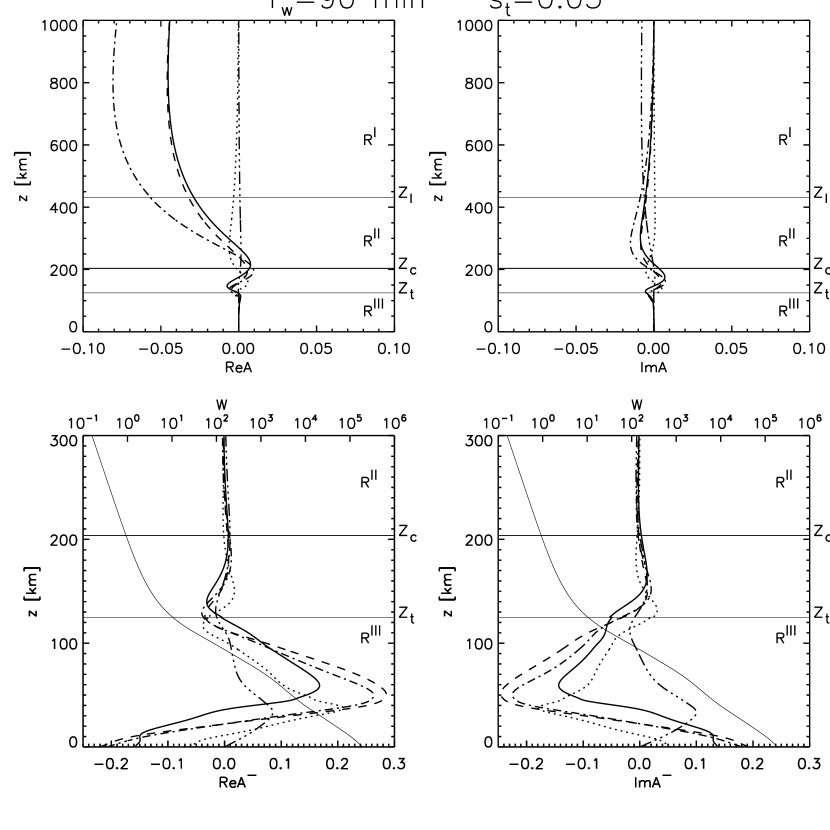
Figure 6: The full structure of a waveguide solution for the period $T_{w}=90min$ Match of lines with wave values is the same as in Figure 6 in Dmitrienko and Rudenko (2016) (point – $\Theta^{(}\Theta^{-})$; dash-point-point-point – $v(v^{-})$; solid – $n(n^{-})$; dashed – $f(f^{-})$; dash-point – $u(u^{-})$ ). The thin solid line describes the height distribution of the function $W(z)$.

Dependencies of real and imaginary parts of components of disturbance of Eqs. (16) and ((21) in Dmitrienko and Rudenko (2016)) are reflected in this figure. The top plots show dependence of relative wave disturbances. The bottom plots describe all the details of the waveguide structure which we cannot see on the top plots because of the exponential factor. We see that the relative values are the largest in the upper atmosphere; the absolute ones, in the lower one. Reaching some maximum, the relative values start decreasing due to effect of dissipation. All the values look continuous at the height of $z_{s}$ with the presented scale. The solution discontinuity indicators are sufficiently small in this case:

$$\begin{array}[]{l}\delta_{[\Theta]}=\delta_{[T]},\delta_{[\Theta^{-}]}=0.134,\\ \delta_{[n}=\delta_{[\rho]},\delta_{[n^{-}]}=0.095.\end{array}$$ (17)

Thus, we got a solution close in quality to the solutions for the isothermal model of the atmosphere (see Section 5 in Dmitrienko and Rudenko (2016)) Note that the calculations show that the discontinuity indicators are identical in order for all the dispersion curve points.

The undisturbed temperature (Figure 6), the pressure, the density, and the sound velocity (Figure 7) shown in the bottom of Figure 6 (thin solid line) give the possibility of calculating absolute values of the disturbances at any height.

Figure 7: The height dependencies of undisturbed pressure, density, and sound velocity.

For an indirect test, one can also use a calculation of a numerical parameter similar to that of total vertical dissipation index $\eta$ of (47) in Dmitrienko and Rudenko (2016)) for a isothermal model of the atmosphere. In the isothermal case, $\eta$ is a ratio of the amplitude modulus $T$ at the height of $z_{c}$ to the amplitude modulus $T$ of upwards propagating wave at the same height without accounting for dissipation. If, as in our case, a part of a reflected wave at the height of $z_{c}$ is small, instead of an incident wave without dissipation, we may use a full combination of an incident wave with a reflected one. Proceeding from it, we select $\eta_{calc}$, for the case with an inhomogeneous atmosphere, similar to $\eta$. To calculate this value, we solve a Cauchy problem from the bottom to the top up to the height $z_{c}$ for the system of equations (3), (12), (13) of Case III from Dmitrienko and Rudenko (2016), using $p$ and $v_{z}$ of the DSAS as boundary values on the Earth’s surface. We calculate the value $\eta_{calc}$ as a ratio of the modulus $T$ at the height of $z_{c}$ to the modulus $T$ of the wave solution got at the same height without dissipation. We give an example of such a calculation in Figure 8. This figure confirms once more that the noticeable distinctions between the solutions with and without dissipation begin with the height $z_{s}$. It can be seen that these solutions significantly differ at the height of $z_{c}$.

Figure 8: The comparison of the waveguide solutions with and without dissipation.

We compare the values of $\eta_{calc}$ and $\eta$ calculated in the theory for the isothermal model where the backgraund temperature is chosen of $T_{0}$ in the non-isothermal model at the height of $z_{c}$. A comparison result of these values in the $0$-mode spectrum is shown in Figure 9.

Figure 9: The comparison of $\eta_{calc}$ and $\eta$.

The last figure shows order of the vertical total dissipation index within the interval $z=[-\infty,z_{c}]$; $\eta(-\infty,z_{c})\approx\eta(z_{s},z_{c})$. The fact that $\eta_{calc}$ is close to isothermal $\eta$ is an essential confirmation of the correctness of the DSAS. Note that if the values $\eta_{calc}$ , $\eta$ are defined through the complex values of their definiens, the complex $\eta_{calc}$ , $\eta$ coincide with each other roughly with the same precision. We do not give the results of calculations for the complex $\eta_{calc}$ , $\eta$.

For a more complete understanding of a waveguide mode, we present three more figures, Figures 10-12, for $T_{w}=180min$ and extreme points of the spectral range $T_{w}=15min$ and $T_{w}=400min$.

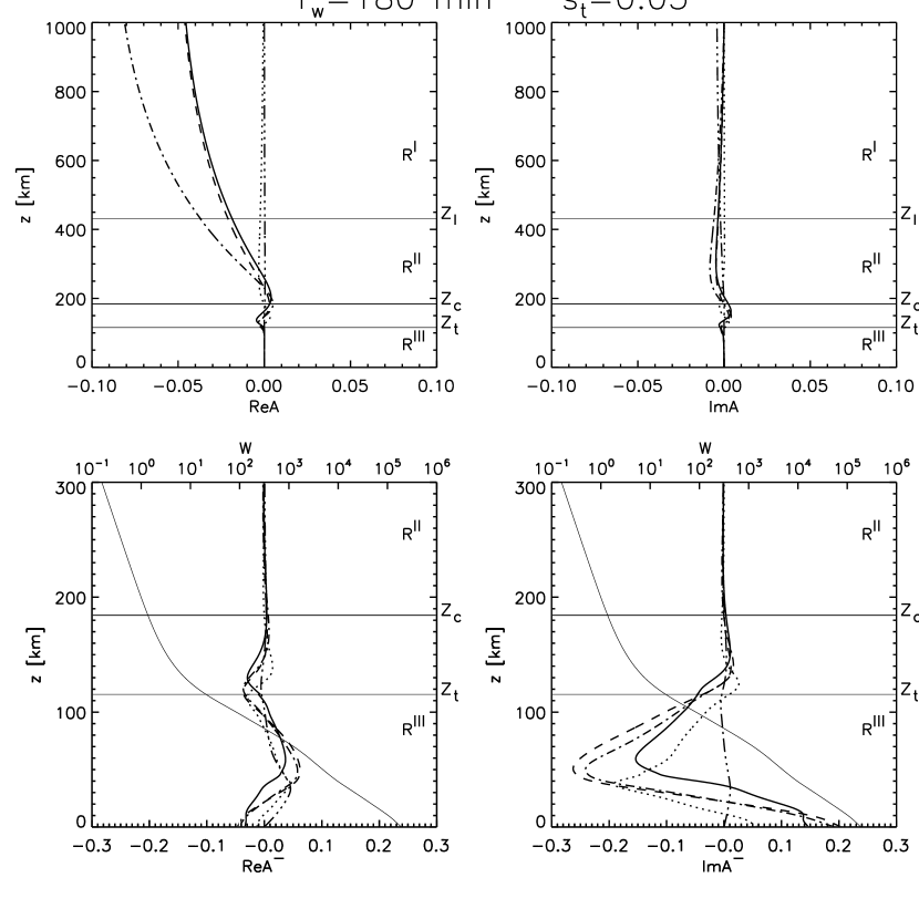
Figure 10: The complete structure of a waveguide solution for the period $T_{w}=180min$.

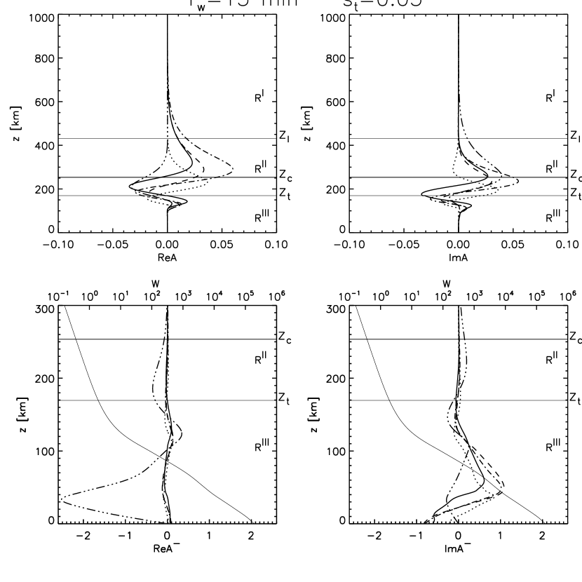
Figure 11: The complete structure of a waveguide solution for the period $T_{w}=15min$.

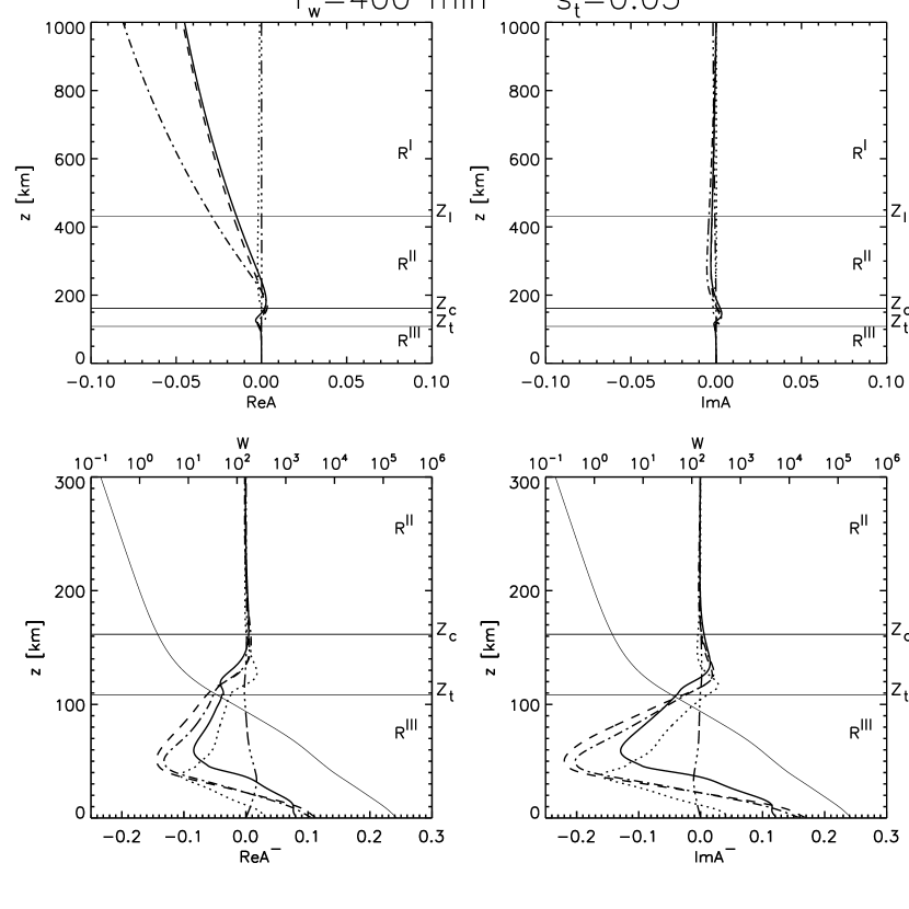
Figure 12: The complete structure of a waveguide solution for the period $T_{w}=400min$.

Note that the longwave spectrum range (Figures 10 -12) does not see discontinuation of the growth of some relative values in the calculated height interval, but it is clear that they attenuate beyond it because the evanescent analytical solutions are continuations of the numerical solutions.

4 Lamb waves

The IGW waveguide modes are not the only of the trapped atmospheric low frequency waves. Surface Lamb waves can be called trapped waves. A domination of pressure, horizontal propagation velocity close to the value of sound velocity near to the Earth’s surface and extremely weak horizontal attenuation Gossard and Hooke (1975) are typical of these waves. The DSAS method has turned to be suitable for description of such modes. The results obtained for Lamb waves are presented in Figures 13-17.

Figure 13: The dispersive relation for a Lamb mode.

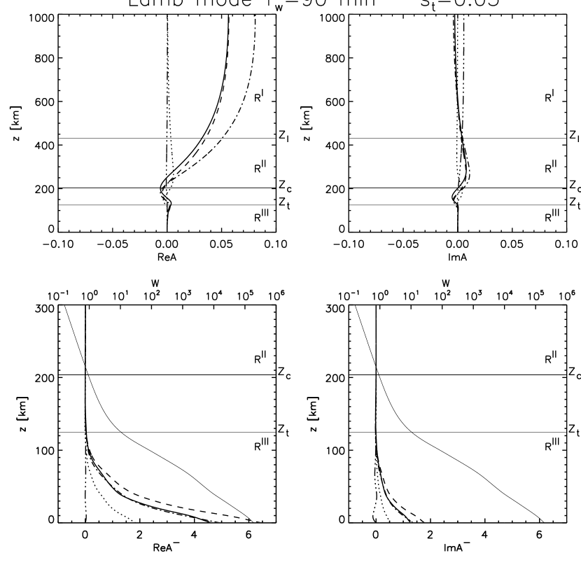
Figure 14: The Lamb wave with the period $T_{w}=90min$.

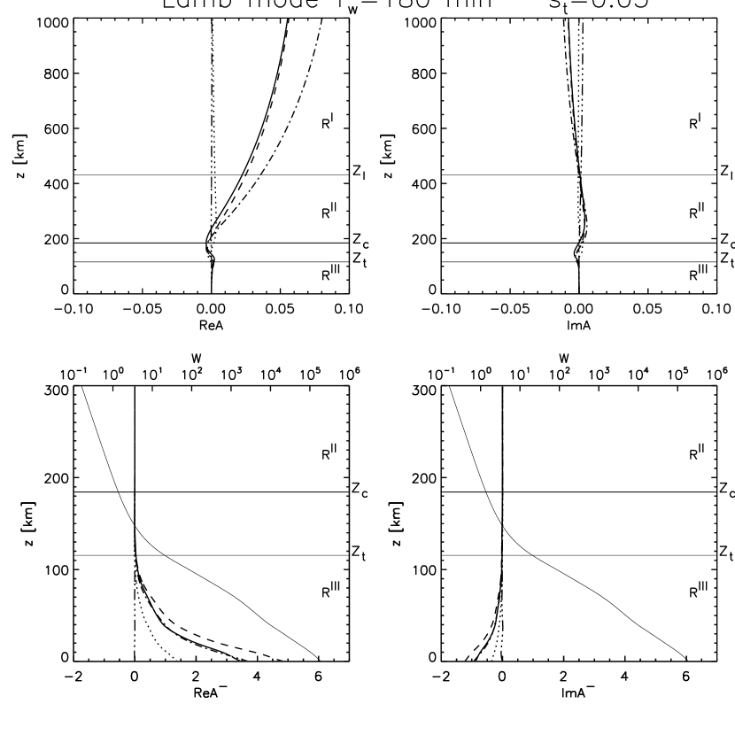
Figure 15: The Lamb wave with the period $T_{w}=180min$.

Figure 16: The Lamb wave with the period $T_{w}=15min$.

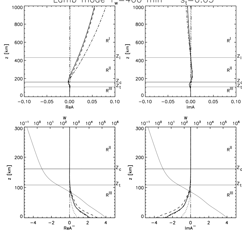
Figure 17: The Lamb wave with the period $T_{w}=400min$.

We do not give the dependence between the horizontal attenuation parameter and period. Predictably, a ratio $\frac{{\rm Im}k_{x}}{{\rm Re}k_{x}}\approx 1.5\times 10^{-5}$ is extremely small with little variations throughout the spectrum. Figures 14-17 give a presentation of the wave structure of a Lamb mode, the same as in Figure 6, 10-12. From the last figures, we see clear domination of a pressure component (dotted lines.) Besides, we see that, despite exponential attenuation of a mode in the lower atmosphere, the upper atmospheric amplitudes of relative values strongly rise, on the contrary, relative to the lower atmosphere. Thus, this mode can be present at the ionospheric heights.

It is also possible to satisfy the conditions of trap for the infrasonic waves higher the sound cutoff frequency. Dispersion of such modes has been analyzed in the WKB-approximation (see, for example, Ponomarev et. al. (2006)) Unlike IGWs, the infrasonic waveguides have a multimode character and divides in their localization place in the lower or middle atmosphere. The waveguide signals of such a type are also widely represented in real disturbances in the lower and middle atmosphere. Analysis of such modes based on the solutions above a source can be also carried out and is quite possible as a subject of our method development; however, these modes deserve separate consideration because of the variety of their characteristics and features.

5 Conclusion

We have studied low frequency trapped waves such as IGW waveguide modes and surface Lamb waves based on the DSAS method.

We have focused on the waveguide solutions corresponding to trapped waves like IGWs. The so-called wave leakage to the upper atmosphere is typical of such trapped waves. Because of an exponential factor typical of the atmospheric waves, upward disturbance exponentially grows in its relative values. The latter leads to the fact that trapped waves are strongly manifested at large heights causing ”visible” travelling ionospheric disturbances (TIDs) to large distances. For the model of the atmosphere that we chose, we have obtained that we had only one fundamental (nodeless) mode at the set frequency. We have calculated a dispersion curve for an IGW waveguide, a complex horizontal number curve as a frequency function. For the first time, we have fully described a vertical structure of an IGW mode at all the heights together with its part leaking from a waveguide and fully accounting for dissipation. We have obtained such a possibility thanks to use of the method for the DSAS (Dmitrienko and Rudenko, 2016) construction. This paper has also revealed that a dissipationless description turned sufficiently useful in the lower atmosphere. It allows us to estimate the number of modes and obtain testing values for a numerical calculation of the eigenvalues. The WKB method is the most convenient for these purposes. It is interesting to note that the WKB description gives correct results, despite its formal inapplicability, with a good coincidence of the WKB dispersion dependences with the exact ones.

Using the obtained dispersion and wave propagation characteristics of the leakage disturbance, we have obtained a very good match with the major characteristics of the observed TIDs: a correlation of horizontal scales with wave periods, propagation ability to many thousands of kilometers without significant attenuation; reverse direction of vertical phase velocity; small values of vertical phase velocity; specific inclination of the phase front.

The dispersive characteristics and complete spatial description of vertical wave structure have been also obtained for Lamb waves.

We believe that a possibility of calculating an adequate vertical structure in case of trapped waves have to give a possibility of tracing atmospheric disturbances at its high frequencies, including, in the ionosphere, with long distance propagation of these disturbances.

Acknowledgment We are grateful to Dr A.V. Medvedev and Dr K.G. Ratovsky for helpful discussion in the course of writing this paper.

References

- Afraimovich at. al. (2001) Afraimovich, E. L., Kosogorov, E. A., Lesyuta, O. S., Ushakov, I. I., Yakovets Network, A. F. 2001. Geomagnetic control of the spectrum of traveling ionospheric disturbances based on data from a global GPS network. Annales Geophysicae, Volume 19, Issue 7, 2001, pp.723-731, doi: 10.5194/angeo-19-723-2001.
- Dmitrienko and Rudenko (2016) Dmitrienko, I. S., Rudenko, G. V., 2016. Waves in vertically inhomogeneous dissipative atmosphere. [arXiv:1440.702].
- Francis (1973a) Francis, S. H. 1973a. Acoustic-gravity modes and large-scale traveling ionospheric disturbances of a realistic, dissipative atmosphere, J.Geophys. Res., 78, 2278.
- Francis (1973b) Francis, S. H. 1973b. Lower-atmospheric gravity modes and their relation to mediumscale traveling ionospheric disturbances, J. Geophys. Res., 78, 8289-8295.
- Heale at. al. (2014) Heale, C. J., Snively, J. B., Hickey, M. P., Ali, C. J. 2014 Thermospheric dissipation of upward propagating gravity wave packets. Journal of Geophysical Research: Space Physics, Volume 119, Issue 5, pp. 3857-3872, doi: 10.1002/2013JA019387.
- Hedlin at. al. (2014) Hedlin, Michael A. H.; Drob, Douglas P. 2014. Statistical characterization of atmospheric gravity waves by seismoacoustic observations. Journal of Geophysical Research: Atmospheres, Volume 119, Issue 9, pp. 5345-5363, doi: 10.1002/2013JD021304.
- Hines (1960) Hines, C. O. 1960. Internal atmospheric gravity waves at ionospheric heights, Can. J. Phys., 38, 1441-1481.
- Gossard and Hooke (1975) Gossard, E. E. and Hooke, W. H. 1975. Waves in the Atmosphere, Elsevier Scientific Publishing Company, New York, 456 pp.
- Medvedev at. al. (2009) Medvedev, A. V., Ratovsky, K. G., Tolstikov, M. V, Kushnarev, D. S. 2009. Method for Studying the Spatial Temporal Structure of Wave-Like Disturbances in the Ionosphere. Geomagnetism and Aeronomy.49(6), 775-785.
- Medvedev at. al. (2013) Medvedev, A. V., Ratovsky, K. G., Tolstikov, M. V, Alsatkin, S. S., Scherbakov, A. A. 2013. Studying of the spatial-temporal structure of wavelike ionosphericdisturbances on the base of Irkutsk incoherent scatter radar and Digisonde data. Journal of Atmospheric and Solar-Terrestrial Physics 105-106, 350-357.
- Ponomarev et. al. (2006) Ponomarev, E. A., Rudenko, G. V., Sorokin, A. G., Dmitrienko, I. S., Lobycheva, I. Yu., Baryshnikov, A. K. 2006. Using the normal-mode method of probing the infrasonic propagation for purposes of the comprehensive nuclear-test-ban treaty. Journal of Atmospheric and Solar-Terrestrial Physics 68, 599-614.
- Ratovsky at. al. (2008) Ratovsky, K. G., Medvedev, A. V., Tolstikov, M. V., Kushnarev, D. S. 2008. Case studies of height structure of TID propagation characteristics using cross-correlation analysis of incoherent scatter radar and DPS-4 ionosonde data. Adv. Space Res. 41, 1453-1457.
- Shibata and Okuzawa (1983) Shibata, T., Okuzawa, T. 1983. Horizontal velocity dispersion of medium-scale travelling ionospheric disturbances in the F-region. Journal of Atmospheric and Terrestrial Physics (ISSN 0021-9169), vol. 45, Feb.-Mar., p. 149-159.
- Vadas and Liu (2009) Vadas, Sharon L., Liu, Han-li. 2009. Generation of large-scale gravity waves and neutral winds in the thermosphere from the dissipation of convectively generated gravity waves. Journal of Geophysical Research, Volume 114, Issue A10, CiteID A10310, doi: 10.1029/2009JA014108.
- Vadas and Nicolls (2012) Vadas, S. L., Nicolls, M. J. 2012. The phases and amplitudes of gravity waves propagating and dissipating in the thermosphere: Theory. Journal of Geophysical Research, Volume 117, Issue A5, CiteID A05322, doi: 10.1029/2011JA017426.
- Idrus et. al. (2013) Idrus, Intan Izafina; Abdullah, Mardina; Hasbi, Alina Marie; Husin, Asnawi; Yatim, Baharuddin. 2013. Large-scale traveling ionospheric disturbances observed using GPS receivers over high-latitude and equatorial regions. Journal of Atmospheric and Solar-Terrestrial Physics, Volume 102, p. 321-328, doi: 10.1016/j.jastp.2013.06.014.