YGHP-15-06

Semilocal Fractional Instantons

Minoru Eto¹ and Muneto Nitta²

¹ Department of Physics, Yamagata University, Yamagata, 990-8560, Japan
² Department of Physics, and Research and Education Center for Natural Sciences,
Keio University, Hiyoshi 4-1-1, Yokohama, Kanagawa 223-8521, Japan

Abstract

We find semi-local fractional instantons of codimension four in Abelian and non-Abelian gauge theories coupled with scalar fields and the corresponding ${\mathbb{C}}P^{N-1}$ and Grassmann sigma models at strong gauge coupling. They are 1/4 BPS states in supersymmetric theories with eight supercharges, carry fractional (half) instanton charges characterized by the fourth homotopy group $\pi_{4}(G/H)$, and have divergent energy in infinite spaces. We construct exact solutions for the sigma models and numerical solutions for the gauge theories. Small instanton singularity in sigma models is resolved at finite gauge coupling (for the Abelian gauge theory). Instantons in Abelian and non-Abelian gauge theories have negative and positive instantons charges, respectively, which are related by the Seiberg-like duality that changes the sign of the instanton charge.

1 Introduction

Yang-Mills instantons are solutions to self-dual equations of pure Yang-Mills theory in Euclidean four space, playing crucial roles in non-perturbative dynamics of gauge theories in four dimensions, in particular in supersymmetric gauge theories [1]. When some scalar fields are coupled to gauge fields, the gauge symmetry is spontaneously broken in the Higgs phase, where instantons cannot exist stably in the bulk as a consequence of the Derrick’s scaling argument [2]. Instead, they can exist stably inside a non-Abelian vortex; the low-energy effective theory of a non-Abelian vortex in a $U(N)$ gauge theory coupled with $N$ fundamental scalar fields is the ${\mathbb{C}}P^{N-1}$ model in two dimensions [3, 4, 5], in which instantons in the bulk exist as lumps (or sigma model instantons) [6, 7, 8]. Such a composite configuration is a 1/4 BPS state preserving a quarter supersymmetry in supersymmetric theories with eight supercharges [7]. Yang-Mills instantons trapped inside a vortex as sigma model instantons elegantly explain a relation between quantum field theories in two and four dimensions [9, 6]. Instanton charges also exist at intersections of vortices [10]. More general BPS composite configurations containing instantons in supersymmetric theories with eight supercharges were classified in Ref. [11]

In two dimensional sigma models, instantons are lumps characterized by the second homotopy group [12], which is, for the ${\mathbb{C}}P^{N-1}$ model,

$$\pi_{2}({\mathbb{C}}P^{N-1})=\pi_{2}\left(\frac{SU(N)}{SU(N-1)\times U(1)}\right)\simeq\pi_{1}\left(SU(N-1)\times U(1)\right)={\mathbb{Z}}.$$ (1.1)

From the last expression of the homotopy relation, it is found that lumps can be promoted to vortices in gauge theories, which is, for the case of the ${\mathbb{C}}P^{N-1}$ model, a $U(1)$ gauge theory coupled to $N$ complex scalar fields. Such vortices are called semilocal vortices [13, 14], reducing to lumps in strong gauge coupling limit [15]. Lumps in Grassmann sigma models are promoted to non-Abelian vortices in a non-Abelian gauge theory [6, 16, 17]. Other than vortices, possible semilocal solitons were classified [18, 19, 20], including codimension-four instantons in quarternionic sigma models [20].

In this paper, we construct BPS instantons of codimension four that solve a set of 1/4 BPS equations in a $U(1)$ or $U(N)$ gauge theory coupled with scalar fields in four dimensions that reduces to the ${\mathbb{C}}P^{N-1}$ model or Grassmann sigma model. It is a Yang-Mills instanton in the gauge theory, and reduces to a codimension-four sigma model instanton in the ${\mathbb{C}}P^{N-1}$ model for which we give an exact solution. It is characterized by the fourth homotopy group

$$\pi_{4}({\mathbb{C}}P^{N-1})=\pi_{4}\left(\frac{SU(N)}{SU(N-1)\times U(1)}\right)\simeq\pi_{3}\left(SU(N-1)\times U(1)\right)={\mathbb{Z}}.$$ (1.2)

The last expression $\pi_{3}[SU(N-1)]\simeq{\mathbb{Z}}$ denotes the homotopy group for Yang-Mills instantons in gauge fields, in parallel with Eq. (1.1) for vortices, and so our solutions may be called semi-local instantons. Although the energy (action) of our solutions is divergent, this divergence comes from the vortex energy while the instanton charge itself is finite. Vortices are sheets linearly extending to two directions in Euclidean four dimensions, having divergent energy $R^{2}$ with the system size $R$. Our solution is spherical and is accompanied by a cloud of a vortex, giving a divergent energy of the same order. Although the Derick’s scaling argument implies the instability against shrinkage for scalar-field objects and gauge-field objects of codimension four, it is not applied to our solutions because of the divergent energy. We construct exact solutions for the sigma models and numerical solutions for the gauge theories. The Grassmann manifold

$$Gr_{N,M}=\frac{SU(N)}{SU(N-M)\times SU(M)\times U(1)}$$ (1.3)

can be reduced from either $U(M)$ gauge theory or $U(N-M)$ gauge theory with $N$ flavors. The Seiberg-like duality exchanges the gauge groups $U(M)$ and $U(N-M)$ with keeping the number of flavors $N$. To find how the Seiberg-like duality acts on our solutions, we focus on the simplest case of the ${\mathbb{C}}P^{2}$ model; $U(1)$ and $U(2)$ gauge theories reduce to the same ${\mathbb{C}}P^{2}$ model at strong gauge couplings. Our solutions are fractional instantons having $\pm 1/2$ fractional instanton charges with a minus (plus) sign for the (non-)Abelian gauge theory. We find that the Seiberg-like duality flips the sign of the instanton charge. We also find that a small instanton singularity in the sigma models is resolved at finite gauge coupling at least for $U(1)$ gauge theory. Our solution is an instanton for (hyper-)Kähler sigma models, while that in Ref. [20] is for quarternionic Kähler sigma models. Another crucial difference between them is that our solution is BPS.

This paper is organized as follows. In Sec. 2 we give Lagrangian of supersymmetric $U(N)$ gauge theory, 1/4 BPS equations, and their solution in terms of the moduli matrix. In Sec. 3, we present semi-local instanton solutions in the Abelian gauge theory and the ${\mathbb{C}}P^{N-1}$ sigma model. In Sec. 4, we present semi-local instanton solutions in the non-Abelian gauge theory and the Grassmannian sigma model. Sec. 5 is devoted to summary and discussion. In Appendix A we describe the transformation of the topological charge under the Seiberg-like duality.

2 The Model, BPS Equations, and Solutions

2.1 $U(N_{\rm C})$ Gauge Theory and 1/4 BPS Equations

In this section, we introduce $U(N_{\rm C})$ gauge theory in (4+1)-dimensional spacetime with $N_{\rm F}$ Higgs fields in the fundamental representation. By introducing additional $N_{\rm F}$ Higgs fields in the fundamental representation, this theory can also be regarded as the bosonic part of a five-dimensional ${\cal N}=1$ supersymmetric $U(N_{\rm C})$ gauge theory with $N_{\rm F}$ hypermultiplets in the fundamental representation. The fermionic part (and another set of $N_{\rm F}$ Higgs scalars) is irrelevant and is omitted in the following discussion. Then the Lagrangian of the theory takes the form

$${\cal L}={\rm Tr}\left[-\frac{1}{2g^{2}}F_{\mu\nu}F^{\mu\nu}+\mathcal{D}_{\mu}H(\mathcal{D}^{\mu}H)^{\dagger}-\frac{g^{2}}{4}(HH^{\dagger}-c\mathbf{1}_{N_{\rm C}})^{2}\right],$$ (2.1)

where the Higgs fields are expressed as an $N_{\rm C}\times N_{\rm F}$ matrix $H^{rA}~{}(r=1,\cdots,N_{\rm C},~{}A=1,\cdots,N_{\rm F})$. The constants $g$ and $c$ are the gauge coupling constant and the Fayet-Iliopoulos (FI) parameter, respectively. At the vacua (the minima of the potential) of this theory, the Higgs fields $H$ get the vacuum expectation value (vev) and the $U(N)$ gauge symmetry is completely broken. Namely the theory has only the Higgs branch due to the nonzero FI term. The moduli space of the vacua is given by a complex Grassmannian

$$Gr_{N_{\rm F},N_{\rm C}}=\frac{SU(N_{\rm F})}{SU(N_{\rm C})\times SU(N_{\rm F}-N_{\rm C})\times U(1)}.$$ (2.2)

The Abelian case $N_{\rm C}=1$ corresponds to the projective space ${\mathbb{C}}P^{N_{\rm F}-1}\simeq{SU(N_{\rm F})/[SU(N_{\rm F}-1)\times U(1)}$. In the strong gauge coupling limit $g\to\infty$, the model reduces to the Grassmann sigma model with the target space in Eq. (2.2).

Let us introduce the complex coordinates $z$ and $w$, complexified gauge fields and the covariant derivatives by

$$z\equiv x^{1}+ix^{3},\quad w\equiv x^{2}+ix^{4},\quad\partial_{z}\equiv\frac{\partial_{1}-i\partial_{3}}{2},\quad\partial_{w}\equiv\frac{\partial_{2}-i\partial_{4}}{2},\qquad$$ (2.3)

$$W_{z}\equiv\frac{W_{1}-iW_{3}}{2},\quad W_{w}\equiv\frac{W_{2}-iW_{4}}{2},\quad\mathcal{D}_{z}\equiv\frac{\mathcal{D}_{1}-i\mathcal{D}_{3}}{2},\quad\mathcal{D}_{w}\equiv\frac{\mathcal{D}_{2}-i\mathcal{D}_{4}}{2},$$ (2.4)

respectively. The 1/4 BPS equations that we consider in this paper are of the form [6, 7]

$$F_{13}+F_{24}=-\frac{g^{2}}{2}\left(c{\bf 1}_{N_{\rm C}}-HH^{\dagger}\right),\quad F_{12}=F_{34},\quad F_{14}=F_{23},$$ (2.5)

$$\bar{\mathcal{D}}_{z}H=0,\quad\bar{\mathcal{D}}_{w}H=0.$$ (2.6)

These equations can be also derived by using the Bogomol’nyi completion of the energy density:

$$E = \int d^{4}x\ {\rm Tr}\left[\frac{1}{2g^{2}}F^{mn}F_{mn}+\mathcal{D}_{m}H(\mathcal{D}^{m}H)^{\dagger}+\frac{g^{2}}{4}\left(c{\bf 1}_{N_{\rm C}}-HH^{\dagger}\right)^{2}\right]$$ (2.7)

$$= \int d^{4}x\ {\rm Tr}\bigg{[}\frac{1}{g^{2}}\bigg{\{}\left(F_{13}+F_{24}+\frac{g^{2}}{2}\left(c{\bf 1}_{N_{\rm C}}-HH^{\dagger}\right)\right)^{2}+\left(F_{12}-F_{34}\right)^{2}$$

$$+\left(F_{14}-F_{23}\right)^{2}\bigg{\}}+4\bar{\mathcal{D}}_{z}H(\bar{\mathcal{D}}_{z}H)^{\dagger}+4\bar{\mathcal{D}}_{w}H(\bar{\mathcal{D}}_{w}H)^{\dagger}$$

$$+i\left\{\mathcal{D}_{1}H(\mathcal{D}_{3}H)^{\dagger}-\mathcal{D}_{3}H(\mathcal{D}_{1}H)^{\dagger}\right\}+i\left\{\mathcal{D}_{2}H(\mathcal{D}_{4}H)^{\dagger}-\mathcal{D}_{4}H(\mathcal{D}_{2}H)^{\dagger}\right\}$$

$$-\left(F_{13}+F_{24}\right)\left(c{\bf 1}_{N_{\rm C}}-HH^{\dagger}\right)+\frac{1}{2g^{2}}F_{mn}\tilde{F}^{mn}\bigg{]}$$

$$= \int d^{4}x\ {\rm Tr}\bigg{[}\frac{1}{g^{2}}\bigg{\{}\left(F_{13}+F_{24}+\frac{g^{2}}{2}\left(c{\bf 1}_{N_{\rm C}}-HH^{\dagger}\right)\right)^{2}+\left(F_{12}-F_{34}\right)^{2}$$

$$+\left(F_{14}-F_{23}\right)^{2}\bigg{\}}+4\bar{\mathcal{D}}_{z}H(\bar{\mathcal{D}}_{z}H)^{\dagger}+4\bar{\mathcal{D}}_{w}H(\bar{\mathcal{D}}_{w}H)^{\dagger}$$

$$-c\left(F_{13}+F_{24}\right)+\frac{1}{g^{2}}F_{mn}\tilde{F}^{mn}+\partial^{m}J_{m}\bigg{]},$$

where we have defined the current

$$J_{1}\equiv iH\mathcal{D}_{3}H^{\dagger},\quad J_{3}\equiv-iH\mathcal{D}_{1}H^{\dagger},$$

$$J_{2}\equiv iH\mathcal{D}_{4}H^{\dagger},\quad J_{4}\equiv-iH\mathcal{D}_{2}H^{\dagger},$$ (2.8)

and have used the following identity

$${\rm Tr}\left[\partial_{1}J_{1}+\partial_{3}J_{3}\right] = i{\rm Tr}\big{[}\mathcal{D}_{1}H\mathcal{D}_{3}H^{\dagger}-\mathcal{D}_{3}H\mathcal{D}_{1}H^{\dagger}-iHH^{\dagger}F_{13}\big{]},$$

$${\rm Tr}\left[\partial_{2}J_{2}+\partial_{4}J_{4}\right] = i{\rm Tr}\big{[}\mathcal{D}_{2}H\mathcal{D}_{4}H^{\dagger}-\mathcal{D}_{4}H\mathcal{D}_{2}H^{\dagger}-iHH^{\dagger}F_{24}\big{]}.$$ (2.9)

We thus have found the energy bound from below

$$E\geq\int dx^{4}\ {\rm Tr}\left(V_{z}+V_{w}+{\cal I}+\partial^{m}J_{m}\right),$$ (2.10)

where the bound consists of three parts

$$V_{z}=-c{\rm Tr}(F_{13}),\quad V_{w}=-c{\rm Tr}(F_{24}),\quad{\cal I}=\frac{1}{g^{2}}{\rm Tr}\left(F_{mn}\tilde{F}^{mn}\right).$$ (2.11)

It is saturated when the 1/4 BPS equations (2.5) and (2.6) are satisfied. Using the BPS equations, the current is expressed by

$$J_{m}=\frac{1}{2}\partial_{m}{\rm Tr}\left[HH^{\dagger}\right].$$ (2.12)

Under the spacial integrations, we have

$$\int d^{4}x\ {\rm Tr}V_{z} = \int dx^{2}dx^{4}\int dx^{1}dx^{3}\ (-c{\rm Tr}F_{13})=-2\pi ck_{z}S_{w},$$ (2.13)

$$\int d^{4}x\ {\rm Tr}V_{w} = \int dx^{1}dx^{3}\int dx^{2}dx^{4}\ (-c{\rm Tr}F_{24})=-2\pi ck_{w}S_{z},$$ (2.14)

where we introduce negative integers

$$k_{z}=\frac{1}{2\pi}\int dx^{1}dx^{3}\ {\rm Tr}F_{13},\qquad k_{w}=\frac{1}{2\pi}\int dx^{2}dx^{4}\ {\rm Tr}F_{24},$$ (2.15)

and the infinite areas $S_{z}=\int dx^{1}dx^{3}$ and $S_{w}=\int dx^{2}dx^{4}$. We have another topological number, the instanton charge

$$I=\frac{g^{2}}{4\pi^{2}}\int dx^{4}\ {\cal I}.$$ (2.16)

Furthermore, $J_{m}$ goes exponentially rapidly to zero at spacial infinity, leading to $\int dx^{4}\ \partial_{m}J_{m}=0$. In summary, the 1/4 BPS solution has mass

$$E=-2\pi c(k_{z}S_{w}+k_{w}S_{z})+\frac{4\pi^{2}}{g^{2}}I.$$ (2.17)

Note that $k_{z,w}$ is always negative due to our choice of sign when we performed the Bogomol’nyi completion at Eq. (2.7). Therefore, the first two terms, the tension of the vortices, are positive definite. On the other hand, the instanton number $I$ is not restricted to be positive or negative. Below, we will show that $I$ is negative in the Abelian gauge theory while it is positive in the non-Abelian gauge theory. When $I$ is negative, it may be suitable that the instanton charge give a sort of binding energy, rather than a particle.

2.2 Solving 1/4 BPS Equations in Terms of the Moduli Matrix

Let us solve the BPS equations (2.5) and (2.6). Eq. (2.6) can be easily solved by introducing the $N_{\rm C}\times N_{\rm F}$ moduli matrix whose components are holomorphic in both $z$ and $w$ [7, 7]

$$H=S^{-1}H_{0}(z,w),\quad\bar{W}_{z}=-iS^{-1}\bar{\partial}_{z}S,\quad\bar{W}_{w}=-iS^{-1}\bar{\partial}_{w}S,$$ (2.18)

where $S\in GL(N_{\rm C},{\mathbb{C}})$. The last two equations can be rewritten by

$$\bar{\mathcal{D}}_{z}S^{-1}=0,\quad\bar{\mathcal{D}}_{w}S^{-1}=0.$$ (2.19)

The last two equations in Eq. (2.5) are automatically satisfied and insure the integrability of two operators $\bar{\mathcal{D}}_{z}$ and $\bar{\mathcal{D}}_{w}$

$$\left[\bar{\mathcal{D}}_{z},\bar{\mathcal{D}}_{w}\right]=\frac{i}{4}\left[F_{12}-F_{34}+i(F_{14}-F_{23})\right]=0.$$ (2.24)

The last unsolved equation is the first one of (2.5). Let us rewrite it by using a gauge invariant $N_{\rm C}\times N_{\rm C}$ hermite matrix

$$\Omega\equiv SS^{\dagger}.$$ (2.25)

By using $\mathcal{D}S^{-1}=-S^{-1}(\partial\Omega)\Omega^{-1}$, $\mathcal{D}^{\prime}S^{-1}=-S^{-1}(\partial^{\prime}\Omega)\Omega^{-1}$ and the equations (2.20)–(2.23), the field strength $F_{mn}$ can be expressed in terms of $\Omega$ as

$$F_{12}+F_{34}-i(F_{14}+F_{23}) = 4iS^{-1}\bar{\partial}\left[(\partial^{\prime}\Omega)\Omega^{-1}\right]S,$$ (2.26)

$$F_{12}+F_{34}+i(F_{14}+F_{23}) = -4iS^{-1}\bar{\partial}^{\prime}\left[(\partial\Omega)\Omega^{-1}\right]S,$$ (2.27)

$$F_{13} = -2S^{-1}\bar{\partial}\left[(\partial\Omega)\Omega^{-1}\right]S,$$ (2.28)

$$F_{24} = -2S^{-1}\bar{\partial}^{\prime}\left[(\partial^{\prime}\Omega)\Omega^{-1}\right]S,$$ (2.29)

where $F_{34}=F_{12},\ F_{23}=F_{14}$ from the BPS solution. Then the last of the BPS equation can be expressed as

$$\bar{\partial}_{z}\left[(\partial_{z}\Omega)\Omega^{-1}\right]+\bar{\partial}_{w}\left[(\partial_{w}\Omega)\Omega^{-1}\right]=\frac{cg^{2}}{4}\left[{\bf 1}_{N_{\rm C}}-\Omega_{0}\Omega^{-1}\right],$$ (2.30)

that we call the master equation, with

$$\Omega_{0}\equiv c^{-1}H_{0}H_{0}^{\dagger}.$$ (2.31)

The energy density can be expressed as follows

$$t_{\rm v} = V_{z}+V_{w}=\frac{c}{2}\triangle_{4}\log\det\Omega,$$ (2.32)

$${\cal I} = \frac{1}{g^{2}}{\rm Tr}\left(F_{12}F_{34}+F_{14}F_{23}-F_{13}F_{24}\right)$$ (2.33)

$$= \frac{4}{g^{2}}{\rm Tr}\bigg{[}\bar{\partial}_{z}\left\{(\partial_{w}\Omega)\Omega^{-1}\right\}\bar{\partial}_{w}\left\{(\partial_{z}\Omega)\Omega^{-1}\right\}-\ \bar{\partial}_{z}\left\{(\partial_{z}\Omega)\Omega^{-1}\right\}\bar{\partial}_{w}\left\{(\partial_{w}\Omega)\Omega^{-1}\right\}\bigg{]}.$$

3 Semilocal Instantons in Abelian Gauge Theory and the ${\mathbb{C}}P^{N-1}$ Model

3.1 Single spherical solution

As the minimal model admitting a semi-local instanton, let us consider $U(1)$ gauge theory with $N_{\rm F}=3$ charged Higgs fields.

The moduli matrix for a spherically symmetric solution in the ${\mathbb{C}}P^{2}$ model is given by

$$H_{0}(z,w) = \sqrt{c}\,(z,\ w,\ a),$$ (3.1)

where $a$ represent size and phase moduli. This yields

$$\Omega_{0} = r^{2}+|a|^{2},$$ (3.2)

where we have defined complex coordinates by

$$z=re^{i\eta}\cos\xi,\quad w=re^{i\lambda}\sin\xi.$$ (3.3)

with $r\in[0,\infty),\ \xi\in[0,\pi/2],\ \eta\in[0,2\pi),\ \lambda\in[0,2\pi)$. Since the source $\Omega_{0}$ is a function of $r$ only, the master equation (2.30) can be reduced into the following ordinary differential equation for $\Omega(r)=e^{u(r)}$,

$$u^{\prime\prime}+\frac{3u^{\prime}}{r}-g^{2}c\left[1-(r^{2}+|a|^{2})e^{-u}\right]=0.$$ (3.4)

It is worth to point out that if we replace the coefficient 3 in the second term by 1, we obtain the master equation for a BPS semi-local vortex in the Abelian-Higgs model with $N_{\rm F}\geq 2$ in $2+1$ dimensions.

In the sigma model limit $g\to\infty$, the energy density coincides with the vortex charge density, because the contribution to the energy density from the instanton charge density vanishes. At the same time we have the exact solution $\Omega=\Omega_{0}$ to the master equation (2.30). The energy density is then given by

$${\cal E}_{g\to\infty}=t_{\rm v}=\frac{c}{2}\left(\partial_{r}^{2}+\frac{3}{r}\partial_{r}\right)\log\Omega=\frac{2c(r^{2}+2|a|^{2})}{(r^{2}+|a|^{2})^{2}}.$$ (3.5)

The energy density $t_{\rm v}$ is shown in Fig. 1.

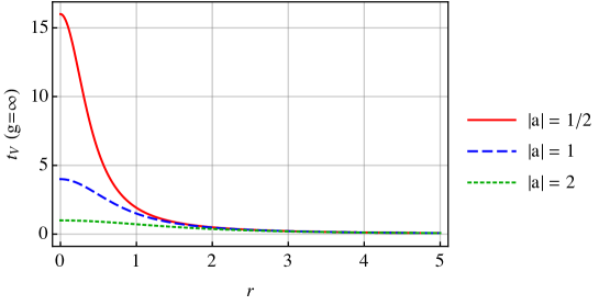
Fig. 1: Energy density $t_{\rm v}$ of one instanton with a size modulus $|a|=1/2,1,2$ at the strong gauge coupling (sigma model) limit $g\to\infty$.

The integrated energy is quadratically divergent $E=\int d^{4}x\,t_{\rm v}\sim R^{2}$ with the size $R$ of the system. The quadratic divergence exists when a vortex is sheet-like, but the same divergence still exists for the spherical configuration that we have constructed. This may be understood as a cloud of a vortex.

The profile functions of the Higgs fields for the exact solution at $g\to\infty$ gives a map from $\mathbb{R}^{4}$ to $\mathbb{C}P^{2}$

$$H(r,\xi,\eta,\lambda)=\sqrt{c}\left(\begin{array}[]{ccc}\dfrac{re^{i\eta}\cos\xi}{\sqrt{r^{2}+|a|^{2}}},&\dfrac{re^{i\lambda}\sin\xi}{\sqrt{r^{2}+|a|^{2}}},&\dfrac{a}{\sqrt{r^{2}+|a|^{2}}}\end{array}\right),$$ (3.7)

where the overall phase is gauged away. Fig. 2 shows the map onto the topic diagram of $\mathbb{C}P^{2}$.

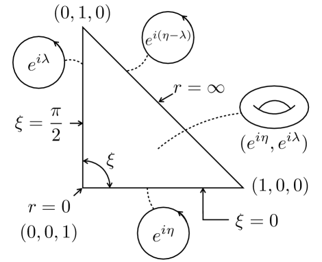
Fig. 2: The map from $\mathbb{R}^{4}$ to $\mathbb{C}P^{2}$. The toric diagram is shown, for which the horizontal and vertical axes denote $|H_{1}|^{2}$ and $|H_{2}|^{2}$, respectively.

At large distance $r\to\infty$, the configuration in Eq. (3.7) reduces to

$$H(r\to\infty,\xi,\eta,\lambda)=\sqrt{c}\left(\begin{array}[]{ccc}e^{i\eta}\cos\xi,&e^{i\lambda}\sin\xi,&0\end{array}\right)\sim\sqrt{c}\left(\begin{array}[]{ccc}e^{i\eta-i\lambda}\cos\xi,&\sin\xi,&0\end{array}\right)$$ (3.10)

where $\sim$ denotes a gauge equivalence. Therefore, the boundary $S^{3}$ at the spacial infinity of $\mathbb{R}^{4}$ is mapped to a submanifold $\mathbb{C}P^{1}\simeq S^{2}$ corresponding to the diagonal edge in Fig. 2. Our configuration therefore has additional topological charge, characterized by the Hopf map

$$\pi_{3}(S^{2})\simeq\mathbb{Z}.$$ (3.11)

Although the instanton charge density at $g\to\infty$ does not contribute to the total energy density, $g^{2}{\cal I}$ has a nonzero support around the origin as is given by

$$g^{2}{\cal I}=-\frac{4|a|^{2}}{\left(r^{2}+|a|^{2}\right)^{3}}.$$ (3.12)

The instanton charge density is shown in Fig. 4.

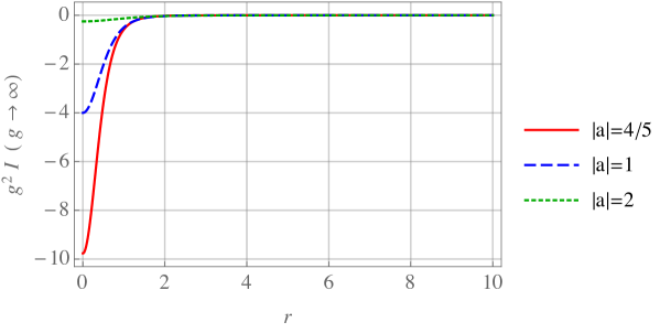
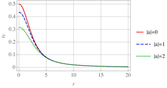
Fig. 3: Instanton charge density $g^{2}{\cal I}$ of a single instanton with a size modulus $|a|=4/5,1,2$ at the strong gauge coupling (sigma model) limit $g\to\infty$.

Fig. 4: $t_{\rm v}$ of a single instanton with a size modulus $|a|=0,1,2$ at the finite gauge coupling $g^{2}c=1$.

The instanton charge of this configuration is finite and interestingly fractional as

$$I=\frac{1}{4\pi^{2}}\int d^{4}x\ g^{2}{\cal I}=-\frac{1}{2}.$$ (3.13)

Thus, this is a fractional instanton, or a meron.

The solution at $g\to\infty$ has a small instanton singularity at $a=0$ where the energy density diverges and the instanton charge density becomes a delta function. The small instanton singularity is resolved for the finite gauge coupling constant $g$, because the typical mass scale $g\sqrt{c}$ turns into the theory. This is a good property for $g<\infty$ but we have to pay the cost that the master equation (3.4) cannot be solved analytically anymore.

Here we numerically solve the master equation for finite gauge couplings. In Fig. 4, we show numerical solutions with $|a|=0,1,2$ as examples. Even for $a=0$, no singular behaviors are observed so that the small instanton singularity is resolved. Compared these with the configurations in Fig. 1, it is seen that the energy density distributions of the finite gauge coupling constant tend to be broader and more smeared. We also show the negative instanton charge densities in Fig. 5. Compared to the infinite gauge coupling limit shown in Fig. 4, the peaks of instanton charge densities become very small; They are about 1 %. Remarkably, the instanton charge contribution to the total energy density does not vanish even for $a=0$. Note that setting $a=0$ in Eq. (3.1) implies that the third component of the the Higgs field is 0 everywhere. Namely, the solution for $a=0$ remains a solution for the theory with $N_{\rm F}=2$ for which the moduli space of vacua is $\mathbb{C}P^{1}\simeq S^{2}$.

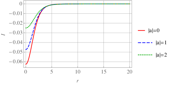
Fig. 5: ${\cal I}$ of the 1 instanton for the finite gauge coupling $g^{2}c=1$.

3.2 Multiple instantons

Non-spherical multiple instantons can be constructed in the ${\mathbb{C}}P^{2}$ model by the moduli matrix of the form of

$$H_{0}=(z^{m}+\cdots,w^{n}+\cdots,a)$$ (3.14)

where $\cdots$ denote polynomials with degrees $m$ of $z$ and $n$ of $w$. This gives

$$\Omega=|z^{m}+\cdots|^{2}+|w^{n}+\cdots|^{2}+a^{2}.$$ (3.15)

For instance, the configuration given by the moduli matrix

$$H_{0}=((z+1.5)(z-1.5),\ w,\,1)$$ (3.16)

is shown in Fig. 6.

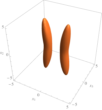
Fig. 6: Sufaces on which $t_{\rm v}=1$ for 2 instantons in $x^{1,2,3}$ space at $x^{4}=0$. We take $c=1$ and $g\to\infty$.

If we go to the ${\mathbb{C}}P^{3}$ model, another spherically symmetric configuration made of four instantons can be constructed. Let us consider the moduli matrix given by

$$H_{0}=(z^{2},w^{2},\sqrt{2}zw,a).$$ (3.17)

This yields

$$\Omega=r^{4}+|a|^{2}.$$ (3.18)

The vortex and instanton charge densities are given by

$$t_{\rm v}=\frac{4r^{2}(r^{4}+3|a|^{2})}{(r^{4}+|a|^{2})^{2}},\quad g^{2}{\cal I}=-\frac{32|a|^{2}\rho^{4}}{\left(r^{4}+|a|^{2}\right)^{3}},$$ (3.19)

respectively. The integrated energy is again quadratically divergent $E\sim R^{2}$ with the system size $R$. As before, although the energy is divergent, the total instanton charge is finite:

$$I=\frac{g^{2}}{4\pi^{2}}\int d^{4}x\ {\cal I}=-2$$ (3.20)

that is four multiple of 1/2 instantons.

4 Semilocal Instantons in Non-Abelian Gauge Theory and the Grassmann Sigma Model

4.1 Single spherical solution

As the simplest case, we consider $U(2)$ gauge theory with $N_{\rm F}=3$ flavors. The moduli space of vacua is

$${\cal M}^{U(2)}_{N_{\rm F}=3}=\frac{SU(3)_{\rm F}}{SU(2)_{\rm C+F}\times U(1)_{\rm C+F}}\simeq{\mathbb{C}}P^{2}$$ (4.1)

which is the same with that of the $U(1)$ gauge theory with $N_{\rm F}=3$ flavors because of the Seiberg-like duality $N_{\rm C}\leftrightarrow N_{\rm F}-N_{\rm C}$. In the strong gauge coupling limit, these two models reduce to the same ${\mathbb{C}}P^{2}$ model.

The moduli matrix of a spherically symmetric solution is given by

$$H_{0}(z,w)=\sqrt{c}\,\left(\begin{array}[]{ccc}1&\dfrac{w}{a}&0\\ 0&z&a\end{array}\right),$$ (4.4)

that gives

$$\Omega_{0}=\left(\begin{array}[]{cc}1+\left|\dfrac{w}{a}\right|^{2}&\dfrac{z^{*}w}{a}\\ \dfrac{zw^{*}}{a^{*}}&|a|^{2}+|z|^{2}\end{array}\right),\quad\det\Omega_{0}=r^{2}+|a|^{2}.$$ (4.7)

This is similar to $\Omega_{0}$ which we encountered in the $U(1)$ gauge theory.

In the strong gauge coupling limit, the master equation is again exactly solved by $\Omega=\Omega_{0}^{-1}$. The profile functions of the Higgs fields are given by

$$S^{-1} = \frac{1}{\sqrt{1+|z|^{2}+|w|^{2}}}\left(\begin{array}[]{cc}\sqrt{1+|z|^{2}}&-\frac{z^{*}w}{\sqrt{1+|z|^{2}}}\\ 0&\sqrt{\frac{1+|z|^{2}+|w|^{2}}{1+|z|^{2}}}\end{array}\right),$$ (4.10)

$$H = \left(\begin{array}[]{ccc}\sqrt{\frac{1+|z|^{2}}{1+|z|^{2}+|w|^{2}}}&\frac{w}{\sqrt{(1+|z|^{2})(1+|z|^{2}+|w|^{2})}}&-\frac{z^{*}w}{\sqrt{(1+|z|^{2})(1+|z|^{2}+|w|^{2})}}\\ 0&\frac{z}{\sqrt{1+|z|^{2}}}&\frac{1}{\sqrt{1+|z|^{2}}}\end{array}\right).$$ (4.13)

Consider $SU(2)_{C}$ invariant quantities, the determinants of 2 by 2 submatrices taking $i$ and $j$-th column from $H$, are given by

$$\det H_{12}=\frac{z}{\sqrt{1+|z|^{2}+|w|^{2}}},\ \det H_{23}=\frac{w}{\sqrt{1+|z|^{2}+|w|^{2}}},\ \det H_{13}=\frac{1}{\sqrt{1+|z|^{2}+|w|^{2}}}.$$ (4.14)

This is exactly identical to the solution in the Abelian theory given in Eq. (3.7). From these we can calculate the instanton density

$$g^{2}{\cal I}=\frac{4a^{2}}{(r^{2}+a^{2})^{3}},$$ (4.15)

that coincides with the one of Eq. (3.12) with opposite sign. Thus, we have a positive contribution $I$ to the energy density,

$$I=\frac{1}{4\pi^{2}}\int dx^{4}\ g^{2}{\cal I}=\frac{1}{2}.$$ (4.16)

The sign flip between the instanton charges in the original theory with $N_{\rm C}$ and the dual theory $N_{\rm C}=N_{\rm F}-N_{\rm C}$ is shown in Appendix A.

On the other hand, we numerically solve the master equation for the finite gauge coupling constant. For simplicity, we will consider the moduli matrix (4.4) with $a=1$. In terms of the complex coordinate coordinates in Eq. (3.3), we have

$$\Omega_{0}=\frac{2+r^{2}}{2}{\bf 1}_{2}+\frac{r^{2}}{2}\left(\begin{array}[]{cc}-\cos 2\xi&e^{i(\lambda-\eta)}\sin 2\xi\\ e^{-i(\lambda-\eta)}\sin 2\xi&\cos 2\xi\end{array}\right).$$ (4.19)

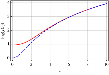
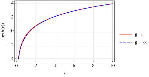
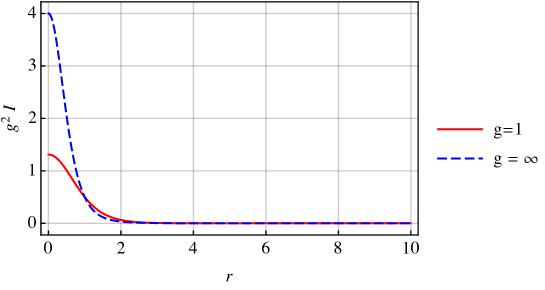
Fig. 7: Profile functions $\log f(r)$ and $\log h(r)$ are shown with $cg^{2}=1,\infty$ for $a=1$.

Fig. 8: Instanton charge densities $g^{2}{\cal I}$ are shown with $cg^{2}=1,\infty$ for $a=1$.

Since $\Omega$ should asymptotically close to $\Omega_{0}$, we make an Ansatz for $\Omega$

$$\Omega=f(r){\bf 1}_{2}+h(r)\left(\begin{array}[]{cc}-\cos 2\xi&e^{i(\lambda-\eta)}\sin 2\xi\\ e^{-i(\lambda-\eta)}\sin 2\xi&\cos 2\xi\end{array}\right),$$ (4.22)

where we impose

$$f(r)\to\frac{2+r^{2}}{2},\quad h(r)\to\frac{r^{2}}{2},\qquad(r\to\infty).$$ (4.23)

Plugging the above Ansatz into the master equation (2.30), we get the following two ordinary differential equations

$$f^{\prime\prime}+\frac{3}{r}f^{\prime}-\frac{1}{r^{2}}\frac{8h^{2}}{f+h}-\frac{ff^{\prime}{}^{2}-2hf^{\prime}h^{\prime}+fh^{\prime}{}^{2}}{f^{2}-h^{2}}+\frac{cg^{2}}{2}\left(2+r^{2}-2f\right)=0,$$ (4.24)

$$h^{\prime\prime}+\frac{3}{r}h^{\prime}-\frac{1}{r^{2}}\frac{8fh}{f+h}+\frac{hf^{\prime}{}^{2}-2ff^{\prime}h^{\prime}+hh^{\prime}{}^{2}}{f^{2}-h^{2}}+\frac{cg^{2}}{2}\left(r^{2}-2h\right)=0.$$ (4.25)

A numerical solution is shown in Fig. 8. The profile functions at the finite gauge coupling are slightly different only near the origin from those at the infinite gauge coupling limit. We also plot the instant charge density $g^{2}{\cal I}$ in Fig. 8. The density $g^{2}{\cal I}$ with $g=1$ becomes slightly smaller than that with $g=\infty$. The peak of the density with $g=1$ is just 1/3 of that with $g=\infty$, which is quite different from the Abelian case seen in the previous subsection.

4.2 Seiberg-like duality

In Figs. 10 and 10, we compare the instanton densities $g^{2}{\cal I}$ of the Abelian and non-Abelian models for the finite gauge coupling $g=1$ and $g=\infty$. Due to the duality $N_{\rm C}\leftrightarrow N_{\rm F}-N_{\rm C}$ shown in Appendix A, Fig. 10 clearly shows that the instanton charge densities at the infinite gauge coupling limit obey the exact relation $g^{2}{\cal I}_{N_{\rm C}=2,N_{\rm F}=3}=-g^{2}{\cal I}_{N_{\rm C}=2,N_{\rm F}=3}$.

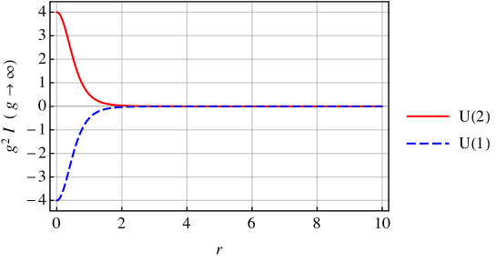
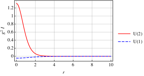
Fig. 9: Instanton charge densities $g^{2}{\cal I}$ with $cg^{2}=\infty$ for $a=1$.

Fig. 10: Instanton charge densities $g^{2}{\cal I}$ with $cg^{2}=1$ for $a=1$.

5 Summary and Discussion

We have studied 1/4 BPS equations and have constructed semi-local fractional instantons of codimension four in $U(N_{\rm C})$ gauge theories with $N_{\rm F}$ scalar fields in Euclidean four dimensions or the corresponding ${\mathbb{C}}P^{N_{\rm F}-1}$ and Grassmann sigma models in strong gauge coupling limit. In the sigma model limit, we have presented exact solutions, and for finite gauge coupling we have given numerical solutions. They have divergent energy in systems with infinite volume $R\to\infty$ as global solitons. We find that they carry fractional instanton charge $(-)1/2$ in non-Abelian (Abelian) gauge theories, and that the Seiberg-like duality changes the sign of the instanton charge.

The topological origin of the fractionality of the topological charge is yet to be clarified. Only when the spatial boundary is mapped to one point on the target space, the topological charge is integer. One known origin of the fractional topological charges is due to the presence of suitable potential term. For instance, a lump (sigma model instanton) in the ${\mathbb{C}}P^{N-1}$ model characterized by $\pi_{2}$ is split into $N$ fractional ($1/N$) lumps [22], and a Skyrmion in the Skyrme model characterized by $\pi_{3}$ is split into two half Skyrmions [23] in the presence of potential terms. The other known example is given by twisted boundary conditions along a compactified direction. There appear $1/N$ fractional lumps (sigma model instantons) of $\pi_{2}$ in the ${\mathbb{C}}P^{N-1}$ model on ${\mathbb{R}}^{1}\times S^{1}$ [7, 24], fractional Grassmann lumps [25] on ${\mathbb{R}}^{1}\times S^{1}$, fractional instantons of $\pi_{N-1}$ in the $O(N)$ model on ${\mathbb{R}}^{N-2}\times S^{1}$ [26], and $1/N$ fractional instantons of $\pi_{3}$ in the $SU(N)$ principal chiral model on ${\mathbb{R}}^{2}\times S^{1}$ [27]. These two cases stabilize fractional charges by either the potential term or the boundary conditions. Our new solitons are stabilized by different mechanism, namely by the topological charges of vortices. A common point for these three cases is that fractional solitons have additional topological charges of one less dimensions. In our case it is the Hopf charge in Eq. (3.11).

A 1/2 BPS non-Abelian vortex in the $U(N)$ gauge theory has the ${\mathbb{C}}P^{N-1}$ moduli space [3, 4]. In 5+1 dimensions a vortex has 3+1 dimensional world-volume. If we consider our instanton solution in the ${\mathbb{C}}P^{N-1}$ model on the Euclid world-volume of the vortex, we have an instanton of codimension four inside a vortex of codimension two. This object of codimension six may be 1/8 BPS state in Euclidean six dimensional theory with eight supercharges [11].

As the other coset spaces that admits the same semilocal instantons, we may consider the followings:

$$\pi_{4}\left(\frac{SO(2N)}{SU(N)\times U(1)}\right)=\pi_{3}\left(SU(N)\times U(1)\right)={\mathbb{Z}},$$ (5.1)

$$\pi_{4}\left(\frac{USp(2N)}{SU(2)\times U(1)}\right)=\pi_{3}\left(SU(N)\times U(1)\right)={\mathbb{Z}}.$$ (5.2)

The nonlinear sigma models with these target spaces can be constructed in supersymmetric gauge theories with suitable superpotentials in the case of four supercharges [28]. These sigma model also appear as the effective theory on a non-Abelian vortex in $G=SO,USp$ gauge theories [29].

It is interesting to take quantum effects into account, although, in this paper, we have focused our attention to the classical aspects of the fractional semilocal instantons. We have taken the common gauge coupling constant $g$ for the $U(1)$ and $SU(N_{\rm C})$ parts for usefulness. The overall $U(1)$ would be free in the IR for the five dimensions, so we may need to solve the equations of motion with different gauge couplings for the $U(1)$ and $SU(N_{\rm C})$ parts. It would modify the solutions obtained in this paper but the qualitative features like topological charges and masses may not be affected.

Appendix A Topological Charges in Seiberg-like Duality

In this section, we discuss the transformation of the topological charge under the Seiberg-like duality. We show that the sign of the topological is flipped.

Let us consider the strong gauge coupling limit $g^{2}\rightarrow\infty$. In this case, there is a duality between the theory with $(N_{\rm F},N_{\rm C})$ and with $(N_{\rm F},\tilde{N}_{\rm C}\equiv N_{\rm F}-N_{\rm C})$. We introduce the dual scalar fields $\tilde{H}$ in the form of an $\tilde{N}_{\rm C}\times N_{\rm F}$ matrix. The scalar fields satisfy the constraints

$$HH^{\dagger}=c{\bf 1}_{N_{\rm C}},\quad\tilde{H}\tilde{H}^{\dagger}=c{\bf 1}_{\tilde{N}_{\rm C}}.$$ (A.1)

Then, there is the following relation between the original fields $H$ and the dual field $\tilde{H}$:

$$H\tilde{H}^{\dagger}=0\quad{\rm or}\quad H^{\dagger}H+\tilde{H}^{\dagger}\tilde{H}=c{\bf 1}_{N_{\rm F}}.$$ (A.2)

The tension of the instanton is given by

$$g^{2}T_{\rm Instanton}=\int d^{4}x\ \frac{1}{2}{\rm Tr}\left(\varepsilon^{MNKL}F_{MN}F_{KL}\right),$$ (A.3)

where the gauge field is expressed as

$$W_{M}=\frac{i}{c}\partial_{M}HH^{\dagger},\quad\tilde{W}_{M}=\frac{i}{c}\partial_{M}\tilde{H}\tilde{H}^{\dagger}.$$ (A.4)

The field strength is then expressed as

$$F_{MN} = \partial_{M}W_{N}-\partial_{N}W_{M}+i\left[W_{M},W_{N}\right]$$ (A.5)

$$= \frac{i}{c}\left[\partial_{M}\left\{\partial_{N}HH^{\dagger}\right\}-\partial_{N}\left\{\partial_{M}HH^{\dagger}\right\}\right]-\frac{i}{c^{2}}\left[\partial_{M}HH^{\dagger},\partial_{N}HH^{\dagger}\right]$$

$$= -\frac{2i}{c}\left[\partial_{[M}H\partial_{N]}H^{\dagger}+\frac{1}{c}\partial_{[M}HH^{\dagger}\partial_{N]}HH^{\dagger}\right]$$

$$= -\frac{2i}{c}\left[\partial_{[M}H\partial_{N]}H^{\dagger}-\frac{1}{c}\partial_{[M}HH^{\dagger}H\partial_{N]}H^{\dagger}\right]$$

$$= -\frac{2i}{c}\left[\partial_{[M}H\partial_{N]}H^{\dagger}-\frac{1}{c}\partial_{[M}H\left(c{\bf 1}_{N_{\rm F}}-\tilde{H}^{\dagger}\tilde{H}\right)\partial_{N]}H^{\dagger}\right]$$

$$= -\frac{2i}{c^{2}}\partial_{[M}H\tilde{H}^{\dagger}\tilde{H}\partial_{N]}H^{\dagger}$$

$$= \frac{2i}{c^{2}}\partial_{[M}H\tilde{H}^{\dagger}\partial_{N]}\tilde{H}H^{\dagger}.$$

where we have defined

$$\partial_{[M}X\partial_{N]}Y\equiv\frac{1}{2}\left[\partial_{M}X\partial_{N}Y-\partial_{N}X\partial_{M}Y\right].$$ (A.6)

Plugging equation (A.5) into the equation (A.3), we get

$${\rm Tr}\left(\varepsilon^{MNKL}F_{MN}F_{KL}\right) = -\frac{4}{c^{4}}{\rm Tr}\left[\varepsilon^{MNKL}\partial_{[M}H\tilde{H}^{\dagger}\partial_{N]}\tilde{H}H^{\dagger}\partial_{[K}H\tilde{H}^{\dagger}\partial_{L]}\tilde{H}H^{\dagger}\right]$$ (A.7)

$$= -\frac{4}{c^{4}}{\rm Tr}\left[\varepsilon^{MNKL}\partial_{M}H\tilde{H}^{\dagger}\partial_{N}\tilde{H}H^{\dagger}\partial_{K}H\tilde{H}^{\dagger}\partial_{L}\tilde{H}H^{\dagger}\right]$$

$$= -\frac{4}{c^{4}}{\rm Tr}\left[\varepsilon^{MNKL}\partial_{N}\tilde{H}H^{\dagger}\partial_{K}H\tilde{H}^{\dagger}\partial_{L}\tilde{H}H^{\dagger}\partial_{M}H\tilde{H}^{\dagger}\right]$$

$$= \frac{4}{c^{4}}{\rm Tr}\left[\varepsilon^{MNKL}\partial_{M}\tilde{H}H^{\dagger}\partial_{N}H\tilde{H}^{\dagger}\partial_{K}\tilde{H}H^{\dagger}\partial_{L}H\tilde{H}^{\dagger}\right]$$

$$= -{\rm Tr}\left(\varepsilon^{MNKL}\tilde{F}_{MN}\tilde{F}_{KL}\right)$$

Note that $\tilde{F}_{MN}$ is not the electric-magnetic dual of $F_{MN}$ but is the field strength of $\tilde{W}_{M}$. We thus have found the relation

$$T_{\rm Instanton}+\tilde{T}_{\rm Instanton}=0$$ (A.8)

implying that the instanton charge is flipped under the duality.

The same relation between the monopole charges in the original and dual theories. In the dimensional reduction, the instanton charge can be written as

$${\rm Tr}\left(\varepsilon^{MNKL}F_{MN}F_{KL}\right) = 4{\rm Tr}\left(\varepsilon^{mnk4}F_{mn}F_{k4}\right)$$ (A.9)

$$\rightarrow 4{\rm Tr}\left(\varepsilon^{mnk}F_{mn}{\cal D}_{k}\Xi\right)$$

$$= 8{\rm Tr}\partial_{k}\left({}^{*}\!F^{k}\Xi\right),$$

where we have defined the adjoint scalar field $\Xi(x^{m})=W_{4}$ and have used the Bianchi identity. Therefore, we have

$$T_{\rm Instanton} \rightarrow T_{\rm Monopole},$$ (A.10)

and the relation

$$T_{\rm Monopole}+\tilde{T}_{\rm Monopole}=0.$$ (A.11)

References

- [1] N. Dorey, T. J. Hollowood, V. V. Khoze and M. P. Mattis, “The Calculus of many instantons,” Phys. Rept. 371, 231 (2002) [hep-th/0206063].
- [2] G. H. Derrick, “Comments on nonlinear wave equations as models for elementary particles,” J. Math. Phys. 5, 1252 (1964).
- [3] A. Hanany and D. Tong, “Vortices, instantons and branes,” JHEP 0307, 037 (2003) [hep-th/0306150].
- [4] R. Auzzi, S. Bolognesi, J. Evslin, K. Konishi and A. Yung, “NonAbelian superconductors: Vortices and confinement in N=2 SQCD,” Nucl. Phys. B 673, 187 (2003) [hep-th/0307287].
- [5] M. Eto, Y. Isozumi, M. Nitta, K. Ohashi and N. Sakai, “Moduli space of non-Abelian vortices,” Phys. Rev. Lett. 96, 161601 (2006) [hep-th/0511088]; M. Eto, K. Konishi, G. Marmorini, M. Nitta, K. Ohashi, W. Vinci and N. Yokoi, “Non-Abelian Vortices of Higher Winding Numbers,” Phys. Rev. D 74, 065021 (2006) [hep-th/0607070]; M. Eto, K. Hashimoto, G. Marmorini, M. Nitta, K. Ohashi and W. Vinci, “Universal Reconnection of Non-Abelian Cosmic Strings,” Phys. Rev. Lett. 98, 091602 (2007) doi:10.1103/PhysRevLett.98.091602 [hep-th/0609214].
- [6] A. Hanany and D. Tong, “Vortex strings and four-dimensional gauge dynamics,” JHEP 0404, 066 (2004) [hep-th/0403158].
- [7] M. Eto, Y. Isozumi, M. Nitta, K. Ohashi and N. Sakai, “Instantons in the Higgs phase,” Phys. Rev. D 72, 025011 (2005) [hep-th/0412048].
- [8] M. Eto, Y. Isozumi, M. Nitta, K. Ohashi and N. Sakai, “Solitons in the Higgs phase: The Moduli matrix approach,” J. Phys. A 39, R315 (2006) [hep-th/0602170].
- [9] M. Shifman and A. Yung, “NonAbelian string junctions as confined monopoles,” Phys. Rev. D 70, 045004 (2004) [hep-th/0403149].
- [10] T. Fujimori, M. Nitta, K. Ohta, N. Sakai and M. Yamazaki, “Intersecting Solitons, Amoeba and Tropical Geometry,” Phys. Rev. D 78, 105004 (2008) [arXiv:0805.1194 [hep-th]].
- [11] M. Eto, Y. Isozumi, M. Nitta and K. Ohashi, “1/2, 1/4 and 1/8 BPS equations in SUSY Yang-Mills-Higgs systems: Field theoretical brane configurations,” Nucl. Phys. B 752, 140 (2006) [hep-th/0506257].
- [12] A. M. Polyakov and A. A. Belavin, “Metastable States of Two-Dimensional Isotropic Ferromagnets,” JETP Lett. 22, 245 (1975) [Pisma Zh. Eksp. Teor. Fiz. 22, 503 (1975)].
- [13] T. Vachaspati and A. Achucarro, “Semilocal cosmic strings,” Phys. Rev. D 44, 3067 (1991).
- [14] A. Achucarro and T. Vachaspati, “Semilocal and electroweak strings,” Phys. Rept. 327, 347 (2000) [Phys. Rept. 327, 427 (2000)] [hep-ph/9904229].
- [15] M. Hindmarsh, “Existence and stability of semilocal strings,” Phys. Rev. Lett. 68, 1263 (1992).
- [16] M. Shifman and A. Yung, “Non-Abelian semilocal strings in N=2 supersymmetric QCD,” Phys. Rev. D 73, 125012 (2006) [hep-th/0603134].
- [17] M. Eto, J. Evslin, K. Konishi, G. Marmorini, M. Nitta, K. Ohashi, W. Vinci and N. Yokoi, “On the moduli space of semilocal strings and lumps,” Phys. Rev. D 76, 105002 (2007) [arXiv:0704.2218 [hep-th]].
- [18] G. W. Gibbons, M. E. Ortiz, F. Ruiz Ruiz and T. M. Samols, “Semilocal strings and monopoles,” Nucl. Phys. B 385, 127 (1992) [hep-th/9203023].
- [19] M. Hindmarsh, “Semilocal topological defects,” Nucl. Phys. B 392, 461 (1993) [hep-ph/9206229].
- [20] M. Hindmarsh, R. Holman, T. W. Kephart and T. Vachaspati, “Generalized semilocal theories and higher Hopf maps,” Nucl. Phys. B 404, 794 (1993) [hep-th/9209088].
- [21] Y. He and H. Guo, “Topological defect with nonzero Hopf invariant in Yang-Mills-Higgs model,” Phys. Lett. B 739, 83 (2014) [arXiv:1405.4089 [math-ph]].
- [22] B. J. Schroers, “Bogomolny solitons in a gauged O(3) sigma model,” Phys. Lett. B 356, 291 (1995) [hep-th/9506004]; B. J. Schroers, “The Spectrum of Bogomol’nyi solitons in gauged linear sigma models,” Nucl. Phys. B 475, 440 (1996) [hep-th/9603101]; M. Nitta and W. Vinci, “Decomposing Instantons in Two Dimensions,” J. Phys. A 45, 175401 (2012) [arXiv:1108.5742 [hep-th]].
- [23] S. B. Gudnason and M. Nitta, “Fractional Skyrmions and their molecules,” Phys. Rev. D 91, no. 8, 085040 (2015) [arXiv:1502.06596 [hep-th]].
- [24] G. V. Dunne and M. Unsal, “Resurgence and Trans-series in Quantum Field Theory: The CP(N-1) Model,” JHEP 1211, 170 (2012) [arXiv:1210.2423 [hep-th]]; G. V. Dunne and M. Unsal, “Continuity and Resurgence: towards a continuum definition of the (N-1) model,” Phys. Rev. D 87, 025015 (2013) [arXiv:1210.3646 [hep-th]]; T. Misumi, M. Nitta and N. Sakai, “Neutral bions in the model,” JHEP 1406, 164 (2014) [arXiv:1404.7225 [hep-th]].
- [25] M. Eto, T. Fujimori, Y. Isozumi, M. Nitta, K. Ohashi, K. Ohta and N. Sakai, “Non-Abelian vortices on cylinder: Duality between vortices and walls,” Phys. Rev. D 73, 085008 (2006) [hep-th/0601181]; T. Misumi, M. Nitta and N. Sakai, “Classifying bions in Grassmann sigma models and non-Abelian gauge theories by D-branes,” PTEP 2015, 033B02 (2015) [arXiv:1409.3444 [hep-th]].
- [26] M. Nitta, “Fractional instantons and bions in the O model with twisted boundary conditions,” JHEP 1503, 108 (2015) [arXiv:1412.7681 [hep-th]].
- [27] M. Nitta, “Fractional instantons and bions in the principal chiral model on with twisted boundary conditions,” JHEP 1508, 063 (2015) [arXiv:1503.06336 [hep-th]].
- [28] K. Higashijima and M. Nitta, “Supersymmetric nonlinear sigma models as gauge theories,” Prog. Theor. Phys. 103, 635 (2000) [hep-th/9911139].
- [29] M. Eto, T. Fujimori, S. B. Gudnason, K. Konishi, M. Nitta, K. Ohashi and W. Vinci, “Constructing Non-Abelian Vortices with Arbitrary Gauge Groups,” Phys. Lett. B 669, 98 (2008) [arXiv:0802.1020 [hep-th]]; M. Eto, T. Fujimori, S. B. Gudnason, K. Konishi, T. Nagashima, M. Nitta, K. Ohashi and W. Vinci, “Non-Abelian Vortices in SO(N) and USp(N) Gauge Theories,” JHEP 0906, 004 (2009) [arXiv:0903.4471 [hep-th]]; M. Eto, T. Fujimori, S. B. Gudnason, Y. Jiang, K. Konishi, M. Nitta and K. Ohashi, “Vortices and Monopoles in Mass-deformed SO and USp Gauge Theories,” JHEP 1112, 017 (2011) [arXiv:1108.6124 [hep-th]].