Reduction rules for the maximum parsimony distance on phylogenetic trees

Abstract

In phylogenetics, distances are often used to measure the incongruence between a pair of phylogenetic trees that are reconstructed by different methods or using different regions of genome. Motivated by the maximum parsimony principle in tree inference, we recently introduced the maximum parsimony (MP) distance, which enjoys various attractive properties due to its connection with several other well-known tree distances, such as tbr and spr. Here we show that computing the MP distance between two trees, a NP-hard problem in general, is fixed parameter tractable in terms of the tbr distance between the tree pair. Our approach is based on two reduction rules–the chain reduction and the subtree reduction–that are widely used in computing tbr and spr distances. More precisely, we show that reducing chains to length 4 (but not shorter) preserves the MP distance. In addition, we describe a generalization of the subtree reduction which allows the pendant subtrees to be rooted in different places, and show that this still preserves the MP distance. On a slightly different note we also show that Monadic Second Order Logic (MSOL), posited over an auxiliary graph structure known as the display graph (obtained by merging the two trees at their leaves), can be used to obtain an alternative proof that computation of MP distance is fixed parameter tractable in terms of tbr-distance. We conclude with an extended discussion in which we focus on similarities and differences between MP distance and TBR distance and present a number of open problems. One particularly intriguing question, emerging from the MSOL formulation, is whether two trees with bounded MP distance induce display graphs of bounded treewidth.

1 Introduction

Finding an optimal tree explaining the relationships of a group of species based on datasets at the genomic level is one of the important challenges in modern phylogenetics. First, there are various methods to estimate the “best” tree subject to certain criteria, such as e.g. Maximum Parsimony or Maximum Likelihood. However, different methods often lead to different trees for the same dataset, or the same method leads to different trees when different parameter values are used. Second, the trees reconstructed from different regions of the genome might also be different, even when using the same criteria. In any case, when two (or more) trees for one particular set of species are given, the problem is to quantify how different the trees really are – are they entirely different or do they agree concerning the placement of most species?

In order to answer this problem, various distances have been proposed (see e.g. [24]). A relatively new one is the so-called Maximum Parsimony distance, or MP distance for short, which we denote $d_{\textsc{MP}}$ [14, 19, 21]. This distance (which is a metric) is appealing in part due to the fact that it is closely related to the parsimony criterion for constructing phylogenetic trees, as well as to the Subtree Prune and Regraft (spr) and Tree Bisection and Reconnection (tbr) distances. Indeed, it is shown in [21] that the unit neighbourhood of the MP distance is larger than those of the spr and tbr distances, implying that a hill-climbing heuristic search based on the MP distance will be less likely to be trapped in a local optimum than those based on the spr or tbr distances. Recently, it has been shown that computing the MP distance is NP-hard [14, 19] even for binary phylogenetic trees. For practical purposes it is therefore desirable to determine whether computation of $d_{\textsc{MP}}$ is fixed parameter tractable (FPT). Informally, this asks whether $d_{\textsc{MP}}$ can be computed efficiently when $d_{\textsc{MP}}$ (or some other parameter of the input) is small, irrespective of the number of species in the input trees. We refer to standard texts such as [12] for more background on FPT. Such algorithms are used extensively in phylogenetics, see e.g. [26] for a recent example.

An obvious approach to address this question is to try to kernelize the problem. Roughly speaking, when given two trees, we seek to simplify them as much as possible without changing $d_{\textsc{MP}}$ so that we can calculate the distance for the simpler trees rather than the original ones. Standard procedures that have been used to kernelize other phylogenetic tree distances are the so-called subtree and chain reductions (see, for example, [1, 6, 17]). In this paper we show that the chain reduction preserves $d_{\textsc{MP}}$ and that chains can be reduced to length 4 (but not less). Moreover, we show that a certain generalized subtree reduction, namely one where the subtrees are allowed to have different root positions, also has this property, which extends a result in [21]. Both reductions can be applied in polynomial time.

These new results allow us to leverage the existing literature on tbr distance. Specifically, in [1] Allen and Steel showed that tbr distance, denoted $d_{\textsc{TBR}}$, is NP-hard to compute, by exploiting the essential equivalence of the problem with the Maximum Agreement Forest (maf) problem: they differ by exactly 1. In the same article they showed (again utilizing the equivalence with maf) that computation of $d_{\textsc{TBR}}$ is FPT in parameter $d_{\textsc{TBR}}$. More specifically, it was shown that combining the subtree reduction with the chain reduction (where chains are reduced to length 3, rather than length 4 as we do here) is sufficient to obtain a reduced pair of trees where the number of species is at most a linear function of $d_{\textsc{TBR}}$. Careful reading of the analysis in [1] shows that a linear (albeit slightly larger) kernel is still obtained for $d_{\textsc{TBR}}$ if chains are reduced to length 4 rather than 3. More recently, in [18] an exponential-time algorithm was described and implemented which computes $d_{\textsc{MP}}$ in time $\Theta(\phi^{n}\cdot\text{poly}(n))$ where $n$ is the number of species in the trees and $\phi\approx 1.618...$ is the golden ratio. Combining the results of [1, 18] with the main results of the current paper (i.e. Theorems 3.1 and 4.1) immediately yields the following theorem:

Theorem 1.1.

Let $T_{1}$ and $T_{2}$ be two unrooted binary trees on the same set of species $X$. Computation of $d_{\textsc{MP}}(T_{1},T_{2})$ is fixed parameter tractable in parameter $d_{\textsc{TBR}}=d_{\textsc{TBR}}(T_{1},T_{2})$. More specifically, $d_{\textsc{MP}}(T_{1},T_{2})$ can be computed in time $O(\phi^{c\cdot d_{\textsc{TBR}}}\cdot\emph{poly}(|X|))$ where $\phi\approx 1.618...$ is the golden ratio and $c\leq 112/3$.

The constant 112/3 is obtained by multiplying the bound on the size of the kernel given in [1] ($28\cdot d_{\textsc{TBR}}$) by a factor 4/3, which adjusts for the fact that here chains are reduced to length 4 rather than 3. Note also that Theorem 1.1 does not require us to apply the generalized subtree reduction: the traditional subtree reduction together with the chain reduction is sufficient.

We now summarise the rest of the paper. In the next section we collect some necessary definitions and notations, including a brief description of Fitch’s algorithm which our proofs extensively use. Then in the following three sections we establish the two reductions for the MP distance, that is, the chain reduction and the subtree reduction, and remark that a theoretical variant of Theorem 1.1 could also be attained by leveraging Courcelle’s Theorem [10, 2], extending in a non-trivial way a technique introduced in [20]. Specifically, computation of $d_{\textsc{MP}}(T_{1},T_{2})$ can be formulated as a sentence of Monadic Second Order Logic (MSOL) posited over an auxiliary graph structure known as the display graph. The display graph is obtained by (informally) merging the two trees at their leaves. Crucially, the length of the sentence, and the treewidth of the display graph, are shown to be both bounded as a function of $d_{\textsc{TBR}}$.

We end with an extended discussion in which we focus on similarities and differences between MP distance and TBR distance. From a theoretical perspective the two distances sometimes behave rather differently but in practice $d_{\textsc{MP}}$ and $d_{\textsc{TBR}}$ are often very close indeed. The major open problem that remains is whether computation of $d_{\textsc{MP}}$ is FPT when parameterized by itself. One possible route to this result is via a strengthened MSOL formulation, but this requires a number of challenging questions to be answered. In particular, can the treewidth of the display graph be bounded as a function of $d_{\textsc{MP}}$ (rather than $d_{\textsc{TBR}}$)? This in turn is likely to require new structural results on the interaction between (large grid) minors in the display graph and phylogenetic incongruency parameters.

2 Preliminaries

2.1 Basic definitions

An unrooted binary phylogenetic tree on a set of species (or, more abstractly, taxa) $X$ is a connected, undirected tree in which all internal nodes have degree 3 and the leaves are bijectively labelled by $X$. For brevity we henceforth refer to these simply as trees, and we often use the elements of $X$ to denote the leaves they label. In some cases, we have to consider rooted binary phylogenetic trees instead of unrooted ones. These trees have an additional internal node of degree 2. When referring to such trees, we will talk about rooted trees for short.

For two trees $T_{1}$ and $T_{2}$ on the same set of taxa $X$, we write $T_{1}=T_{2}$ if there is an isomorphism between the two trees that preserves the labels $X$. The expression $T|_{X^{\prime}}$, where $X^{\prime}\subseteq X$, has the usual definition, namely: the tree obtained by taking the unique minimal spanning tree on $X^{\prime}$ and then repeatedly suppressing any nodes of degree 2.

A character on $X$ is a surjective function $f:X\rightarrow\mathbf{C}$ where $\mathbf{C}$ is a set of states. Given a phylogenetic tree $T=(V,E)$ on $X$, and a character $f$ on $X$, an extension of $f$ to $T$ is a mapping $\overline{f}:V\rightarrow\mathbf{C}$ which extends $f$ i.e. for every $x\in X$, $f(x)=\overline{f}(x)$. The number of mutations induced by $\overline{f}$, denoted by $\Delta(\overline{f})$, is defined to be the number of edges $\{u,v\}\in E$ such that $\overline{f}(u)\neq\overline{f}(v)$. The parsimony score of $f$ on $T$ (sometimes called the length) is defined to be the minimum, ranging over all extensions $\overline{f}$ of $f$ to $T$, of the number of mutations induced by $\overline{f}$. This is denoted $l_{f}(T)$. Following [27], an extension $\overline{f}$ that achieves this minimum is called a minimum extension (also known as an optimal extension, but here we reserve the word optimal for other use). This value can be computed in polynomial time using dynamic programming. Fitch’s algorithm is the most well-known example of this. (We will use Fitch’s algorithm extensively in this article and give a brief description of its execution in the next section).

Given two trees $T_{1}$ and $T_{2}$ on $X$, the maximum parsimony distance of $T_{1}$ and $T_{2}$, denoted $d_{\textsc{MP}}=d_{\textsc{MP}}(T_{1},T_{2})$, is defined as

$$d_{\textsc{MP}}(T_{1},T_{2})=\max_{f}|l_{f}(T_{1})-l_{f}(T_{2})|$$

where $f$ ranges over all characters on $X$. A character $f$ that achieves this maximum is called an optimal character. In [14, 21] it is proven that $d_{\textsc{MP}}$ is a metric.

Note that in this manuscript, we also compare $d_{\textsc{MP}}$ to the well-known Tree Bisection and Reconnection (TBR) distance, denoted $d_{TBR}$. Recall that a TBR move is performed as follows: Given an unrooted binary phylogenetic tree, delete one edge and suppress all resulting nodes of degree 2. Of the two trees now present, if they consist of at least two nodes, pick an edge and place a degree-2 node on it and choose it; else if either one only consists of one leaf, choose this leaf. Now connect the two chosen nodes with a new edge. This completes the TBR move. Note that $d_{\textsc{tbr}}(T_{1},T_{2})$ is defined as the minimum number of TBR moves needed to transform $T_{1}$ into $T_{2}$. In [14, 21] it is proven that $d_{\textsc{MP}}(T_{1},T_{2})\leq d_{\textsc{TBR}}(T_{1},T_{2})$ for all trees $T_{1},T_{2}$, with both articles listing examples where the inequality is strict.

A concept which often occurs when discussing tree distances is the so-called agreement forest abstraction. Recall that, given two trees $T_{1}$ and $T_{2}$ on $X$, an agreement forest is a partition of $X$ into non-empty subsets $X_{1},\ldots,X_{k}$, such that $T_{1}|_{X_{i}}$ and $T_{2}|_{X_{i}}$ are isomorphic for all $i$, and such that the subtrees $T_{t}|_{X_{i}}$ and $T_{t}|_{X_{j}}$ are node disjoint subtrees of $T_{t}$ for all $i$ and $j\in\{1,\ldots,k\}$ and for $t=1,2$. An agreement forest with a minimum number of components is called a Maximum Agreement Forest, or MAF for short. In [1] it was proven that $d_{\textsc{TBR}}$ is equal to the number of components in a MAF, minus one.

The last concept we need to recall is fixed parameter tractability (FPT). An algorithm is fixed parameter tractable in parameter $k$ if its running time has the form $g(k)\cdot\text{poly}(n)$ where $n$ is the size of the input (here we take $n=|X|$) and $g$ is some (usually exponential) computable function that depends only on $k$. For distances on trees it is quite usual to take the distance itself as the parameter, but other parameters can be chosen, and this is the approach we take in this article (i.e. we parameterize computation of $d_{\textsc{MP}}$ in terms of $d_{\textsc{TBR}}$). For more formal background on FPT we refer the reader to [12].

We defer a number of definitions (concerning treewidth and display graphs) until later in the article.

2.2 Fitch’s algorithm

For a given character $f$ on $T$, Fitch’s algorithm [15] is a well-known polynomial-time algorithm for computing $l_{f}(T)$ and inferring a minimum extension of $f$ (see, e.g. [28], for a recent application). It has a bottom-up phase followed by a top-down phase (actually, in the original paper, Fitch introduced a second top-down phase, but this is not needed in the present manuscript and is thus ignored here). It works on rooted trees, but the location of the root is not important for computation of $l_{f}(T)$, so we may root the tree by subdividing an arbitrary edge with a new node $\rho$ and directing all edges away from this new node. (In particular, this ensures that the child-parent relation is well-defined). For each internal node $u$ of a rooted tree, let $u_{l}$ and $u_{r}$ refer to its two children.

In the first phase, the algorithm constructs the Fitch map $\mathbf{F}:V(T)\to 2^{\mathbf{C}}\setminus\{\emptyset\}$ (induced by character $f$) that assigns a subset of states to each of node $u$ of $T$ in the following bottom-up approach:

1. For each leaf $x$, let $\mathbf{F}(x)=\{f(x)\}$.

2. For each internal node $u$ (for which $\mathbf{F}(u_{l})$ and $\mathbf{F}(u_{r})$ have already been computed), let

   $$\mathbf{F}(u)=\mathbf{F}(u_{l})*\mathbf{F}(u_{r})=\begin{cases}\mathbf{F}(u_{l})\cup\mathbf{F}(u_{r})&\mbox{if $\mathbf{F}(u_{l})\cap\mathbf{F}(u_{r})=\emptyset$,}\\ \mathbf{F}(u_{l})\cap\mathbf{F}(u_{r})&\mbox{otherwise.}\end{cases}$$ (1)

An internal node $u$ is called a union node if the first case in Equation (1) occurs (i.e., $\mathbf{F}(u_{l})\cap\mathbf{F}(u_{r})=\emptyset$), and an intersection node otherwise. The value $l_{f}(T)$ is equal to the total number of union nodes in $T$.

For later use, an extension $\overline{f}$ of $f$ on $T$ is called a Fitch-extension if (i) $\overline{f}(u)\in\mathbf{F}(u)$ holds for all $u\in V(T)$, and (ii) for each non-leaf node $u$ of $V(T)$, we have either $\overline{f}(u)=\overline{f}(u_{l})$ or $\overline{f}(u)=\overline{f}(u_{r})$ (but not both) if $u$ is a union node, and $\overline{f}(u)=\overline{f}(u_{l})=\overline{f}(u_{r})$ otherwise (i.e. $u$ is an intersection node).

In the second phase, for an arbitrary state $s\in\mathbf{F}(\rho)$ the algorithm constructs a Fitch-extension $\overline{f}$ in the following top-down manner. We start with $\overline{f}(\rho)=s$. Suppose that $v$ is a child of $u$ for which $\overline{f}(u)$ is defined, then

$$\overline{f}(v)=\begin{cases}\overline{f}(u)&\mbox{if $\overline{f}(u)\in\mathbf{F}(v)$,}\\ \mbox{any state in $\mathbf{F}(v)$}&\mbox{otherwise.}\end{cases}$$ (2)

Since each union node will contribute precisely one mutation for the extension $\overline{f}$ specified in Equation (2), each Fitch-extension is always minimum. (However, note that a minimum extension is not necessarily a Fitch-extension [13].) The following observation, which we use later, is immediate from the second phase of Fitch’s algorithm.

Observation 2.1.

Let $T$ be a rooted binary tree on $X$ and let $f$ be a character on $X$. Let $\rho$ be the root of $T$ and consider the Fitch map $\mathbf{F}$ induced by $f$. For each state $s\in\mathbf{F}(\rho)$, there exists a Fitch-extension $\overline{f}$ of $f$ such that $\overline{f}(\rho)=s$.

3 Chain reduction

Let $T$ be an unrooted binary tree on $X$. For a leaf $x_{i}\in X$, let $p_{i}$ denote the internal node of $T$ adjacent to this leaf. Then, an ordered sequence $(x_{1},\ldots,x_{k})$ of $k$ taxa is called a chain of length $k$ if $(p_{1},p_{2},\ldots,p_{k})$ is a path in $T$. Note that here we allow that $p_{1}=p_{2}$ (i.e., $x_{1}$ and $x_{2}$ have a common parent) and/or $p_{k-1}=p_{k}$ (i.e. $x_{k-1}$ and $x_{k}$ have a common parent): if at least one of these situations occurs we say the chain is pendant. (This is equivalent to definitions used in earlier articles). A chain is common to $T_{1}$ and $T_{2}$ if it is a chain of both trees. Suppose $T_{1}$ and $T_{2}$ have a common chain $K=(x_{1},\ldots,x_{k})$ where $X(K)$ denotes the taxa in the chain and $k=|X(K)|\geq 5$. Let $T^{\prime}_{1}$, $T^{\prime}_{2}$ be two new trees on $X^{\prime}=(X\setminus X(K))\cup\{x_{1},x_{2},x_{k-1},x_{k}\}$ where $T^{\prime}_{1}=T_{1}|_{X^{\prime}}$ and $T^{\prime}_{2}=T_{2}|_{X^{\prime}}$. Then we say that $T^{\prime}_{1}$, $T^{\prime}_{2}$ have been obtained by reducing $K$ to length 4.

Theorem 3.1.

Let $T_{1}$ and $T_{2}$ be two unrooted binary trees on the same set of taxa $X$. Let $K$ be a common chain of length $k\geq 5$. Let $T^{\prime}_{1}$ and $T^{\prime}_{2}$ be the two trees obtained by reducing $K$ to length 4. Then $d_{\textsc{MP}}(T_{1},T_{2})=d_{\textsc{MP}}(T^{\prime}_{1},T^{\prime}_{2})$.

Proof.

Note that $d_{\textsc{MP}}(T^{\prime}_{1},T^{\prime}_{2})\leq d_{\textsc{MP}}(T_{1},T_{2})$ follows from Corollary 3.5 of [21], which proves that for all $Y\subseteq X$, $d_{\textsc{MP}}(T_{1}|_{Y},T_{2}|_{Y})\leq d_{\textsc{MP}}(T_{1},T_{2})$. The inequality then follows from the definition of chain reduction.

It is considerably more involved to prove the claim that $d_{\textsc{MP}}(T^{\prime}_{1},T^{\prime}_{2})\geq d_{\textsc{MP}}(T_{1},T_{2})$ holds.

Without loss of generality, we may assume that $d_{\textsc{MP}}(T_{1},T_{2})>0$ (i.e., $T_{1}\not=T_{2}$) as otherwise the claim clearly holds. Note that this implies $X\not=X(K)$ and hence whenever $K$ is pendant in a tree, at least one end of the chain is attached to the main part of the tree.

We will prove the claim by considering the following three major cases: (I) the common chain is pendant in neither tree, (II) the chain is pendant in preciesly one tree, and (III) the chain is pendant in both trees.

I: Common chain is pendant in neither tree

Let $f$ be an optimal character for $T_{1}$ and $T_{2}$ i.e. $|l_{f}(T_{1})-l_{f}(T_{2})|=d_{\textsc{MP}}(T_{1},T_{2})$. Assume without loss of generality that $l_{f}(T_{1})<l_{f}(T_{2})$, so $d_{\textsc{MP}}(T_{1},T_{2})=l_{f}(T_{2})-l_{f}(T_{1})$.

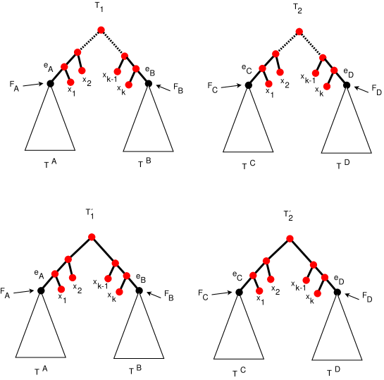
Figure 1: The chain reduction as applied in the case when the common chain $K$ is pendant in neither tree. Note that in $T_{1}$ and $T_{2}$ a dotted line is used to denote the taxa $\{x_{3},\ldots,x_{k-2}\}$ which are removed by the chain reduction. All the trees in the figure are unrooted, but for the purpose of proving correctness of the chain reduction we have shown them as rooted. $T^{\prime}_{1}$ and $T^{\prime}_{2}$ must be rooted exactly halfway along the chain, as shown. For $T_{1}$ and $T_{2}$ it is not so important where the tree is rooted as long as the root is in the same part of the chain in both trees.

Let $T^{A},T^{B},T^{C},T^{D}$ refer to the 4 subtrees of $T_{1},T_{2}$ shown in Figure 1. For $P\in\{A,B,C,D\}$, let $e_{P}$ refer to the edge incoming to the root of $T^{P}$; let $X_{P}$ refer to the taxa in subtree $T^{P}$; let $f_{P}$ denote the character obtained by restricting $f$ to $X_{P}$, and let $\mathbf{F}_{P}$ refer to the set of states assigned to the root of $T^{P}$ by the Fitch map induced by $f_{P}$. (Note that $X_{A}\cup X_{B}=X_{C}\cup X_{D}$.) For each tree $T\in\{T_{1},T_{2},T^{\prime}_{1},T^{\prime}_{2}\}$ we define the chain region of $T$ to be the set of edges incident to at least one red node (as shown in Figure 1). Let $m_{i}$ $(i=1,2)$ be the number of union nodes among red nodes, which is the same as the number of mutations occuring in the chain region of $T_{i}$ for a Fitch-extension of $f$. Then,

$$m_{1} =l_{f}(T_{1})-l_{f_{A}}(T^{A})-l_{f_{B}}(T^{B})~{}\mbox{and}$$

$$m_{2} =l_{f}(T_{2})-l_{f_{C}}(T^{C})-l_{f_{D}}(T^{D}).$$

In addition, let $p=m_{2}-m_{1}$ and then we have

$$d_{\textsc{MP}}(T_{1},T_{2})=l_{f_{C}}(T^{C})+l_{f_{D}}(T^{D})-l_{f_{A}}(T^{A})-l_{f_{B}}(T^{B})+p.$$ (3)

First we shall show that $p\leq 2$. To this end, fix a Fitch-extension $\overline{f}_{1}$ of $f$ to $T_{1}$, and consider an extension $\overline{f_{2}}$ of $f$ to $T_{2}$ obtained by combining a minimum extension of $f_{C}$ to $T^{C}$, a minimum extension of $f_{D}$ to $T^{D}$, and exactly mimicking $\overline{f_{1}}$ on the red nodes of $T_{2}$ (as indicated in Figure 1). Then compared with $\overline{f}_{1}$, the extension $\overline{f}_{2}$ creates at most two new mutations on the chain region (i.e. edges $e_{C}$ and $e_{D}$). In other words, we have $\Delta(\overline{f}_{2})\leq l_{f_{C}}(T^{C})+l_{f_{D}}(T^{D})+(m_{1}+2)$. Together with $l_{f}(T_{2})\leq\Delta(\overline{f}_{2})$ and $l_{f}(T_{1})=l_{f_{A}}(T^{A})+l_{f_{B}}(T^{B})+m_{1}$, this implies

$$p = l_{f}(T_{2})-l_{f}(T_{1})-l_{f_{C}}(T^{C})-l_{f_{D}}(T^{D})+l_{f_{A}}(T^{A})+l_{f_{B}}(T^{B})$$ (4)

$$= l_{f}(T_{2})-m_{1}-l_{f_{C}}(T^{C})-l_{f_{D}}(T^{D})$$

$$\leq \Delta(\overline{f}_{2})-m_{1}-l_{f_{C}}(T^{C})-l_{f_{D}}(T^{D})$$

$$\leq 2.$$

Next we show $p\geq 0$. Consider a new (not necessarily optimal) character $f^{*}$ obtained from $f$ by reassigning all the taxa in $X(K)$ to a new state $s$ that does not appear anywhere on $X\setminus X(K)$. Considering Fitch-extensions of $f^{*}$ to $T_{1}$ and to $T_{2}$ we observe that $T_{1}$ and $T_{2}$ will both incur exactly 2 mutations in their chain regions, namely on edges $e_{A}$, $e_{B}$ and $e_{C}$, $e_{D}$, respectively. That is, we have

$$l_{f^{*}}(T_{1})=l_{f_{A}}(T^{A})+l_{f_{B}}(T^{B})+2~{}~{}\mbox{and}~{}~{}l_{f^{*}}(T_{2})=l_{f_{C}}(T^{C})+l_{f_{D}}(T^{D})+2.$$ (5)

Since the optimality of $f$ implies $l_{f}(T_{2})-l_{f}(T_{1})\geq l_{f^{*}}(T_{2})-l_{f^{*}}(T_{1})$, by Equation (5) we have

$$p = l_{f}(T_{2})-l_{f}(T_{1})-l_{f_{C}}(T^{C})-l_{f_{D}}(T^{D})+l_{f_{A}}(T^{A})+l_{f_{B}}(T^{B})$$ (6)

$$\geq l_{f^{*}}(T_{2})-l_{f^{*}}(T_{1})-l_{f_{C}}(T^{C})-l_{f_{D}}(T^{D})+l_{f_{A}}(T^{A})+l_{f_{B}}(T^{B})$$

$$= 0.$$

By Equation (3), the claim $d_{\textsc{MP}}(T^{\prime}_{1},T^{\prime}_{2})\geq d_{\textsc{MP}}(T_{1},T_{2})$ will follow from

$$d_{\textsc{MP}}(T^{\prime}_{1},T^{\prime}_{2})\geq l_{f_{C}}(T^{C})+l_{f_{D}}(T^{D})-l_{f_{A}}(T^{A})-l_{f_{B}}(T^{B})+p.$$ (7)

Therefore, to establish main case (I) it is sufficient to establish Equation (7), which will be done through case analysis on $p$. To shorten notation we will write $f[a,b,c,d]$ to denote the character on $X^{\prime}$ obtained from $f$ (which is a character on $X$) by leaving the states assigned to taxa in $X_{A}\cup X_{B}=X_{C}\cup X_{D}$ intact and assigning states $a,b,c,d$ to $x_{1},x_{2},x_{k-1},x_{k}$ respectively. (Occasionally we will manipulate $f$ to obtain a new character $f^{*}$ also on $X$, and then the expression $f^{*}=f[a,b,\ldots,c,d]$ is overloaded to denote the reassignment of states to the taxa in the original chain $K$, not the reduced chain.) Since $p$ is an integer with $0\leq p\leq 2$, we have the following three cases to consider.

Case 1: $p=0$. Let $f^{\prime}=f[s,s,s,s]$ where $s$ is a state that does not appear elsewhere. Then by the “both trees incurring exactly 2 mutations in their chain regions for Fitch-extensions” reason used in the proof of Equation (5), we have $l_{f^{\prime}}(T^{\prime}_{2})-l_{f^{\prime}}(T^{\prime}_{1})=l_{f_{C}}(T^{C})+l_{f_{D}}(T^{D})-l_{f_{A}}(T^{A})-l_{f_{B}}(T^{B})$, from which Equation (7) holds.

Case 2: $p=1$. We require a subcase analysis on $\mathbf{F}_{A},\mathbf{F}_{B},\mathbf{F}_{C},\mathbf{F}_{D}$.

1. $\mathbf{F}_{A}\setminus\mathbf{F}_{C}\neq\emptyset$: Let $a\in\mathbf{F}_{A}\setminus\mathbf{F}_{C}$. Consider a state $s$, which is a state that does not appear elsewhere, and the character $f^{\prime}=f[a,s,s,s]$. If we consider Fitch-extensions of $f^{\prime}$ on $T^{\prime}_{1}$ and on $T^{\prime}_{2}$, we see that in $T^{\prime}_{1}$ there are exactly 2 mutations incurred in the chain region, and in $T^{\prime}_{2}$ exactly 3, and we are done, because we now have $l_{f^{\prime}}(T^{\prime}_{1})=l_{f_{A}}(T^{A})+l_{f_{B}}(T^{B})+2$ and $l_{f^{\prime}}(T^{\prime}_{2})=l_{f_{C}}(T^{C})+l_{f_{C}}(T^{C})+3$, so $d_{\textsc{MP}}(T^{\prime}_{1},T^{\prime}_{2})\geq l_{f^{\prime}}(T^{\prime}_{2})-l_{f^{\prime}}(T^{\prime}_{1})=d_{\textsc{MP}}(T_{1},T_{2})$. The latter equality is true because we are in the case where $p=1$. For brevity we henceforth speak of “an $(i,j)$ situation” when there are $i$ mutations in the chain region in tree $T^{\prime}_{1}$ and $j$ in $T^{\prime}_{2}$, so in this case we have a (2,3) situation.

2. $\mathbf{F}_{B}\setminus\mathbf{F}_{D}\neq\emptyset$: This is symmetrical to the previous case.

3. $(\mathbf{F}_{A}\subseteq\mathbf{F}_{C})\wedge(\mathbf{F}_{B}\subseteq\mathbf{F}_{D})$: This case cannot occur. Intuitively, $T_{2}$ is “less constrained” than $T_{1}$ at the roots of the subtrees, so there is no way that $T_{1}$ can use the chain region to save mutations relative to $T_{2}$. More formally, consider a Fitch-extension $\overline{f_{1}}$ of $f$ to $T_{1}$. Then by definition $\overline{f_{1}}$ assigns a state $a$ from $\mathbf{F}_{A}$ to the root of $T_{A}$, and a state $b$ from $\mathbf{F}_{B}$ to the root of $T_{B}$ (where $a$ and $b$ are not necessarily different). Since $a\in\mathbf{F}_{C}$, by Observation 2.1, we fix a Fitch-extension $\overline{f}_{C}$ of $f_{C}$ to $T^{C}$ that maps the root of $T^{C}$ to $a$. Similarly, we fix a Fitch-extension $\overline{f}_{D}$ of $f_{D}$ to $T^{D}$ that maps the root of $T^{D}$ to $b$. Now consider the extension $\overline{f_{2}}$ of $f$ to $T_{2}$ obtained by combining $\overline{f}_{C}$, $\overline{f}_{D}$, and exactly mimicking $\overline{f_{1}}$ for the red nodes of $T_{2}$. Then the number of mutations induced by $\overline{f_{2}}$ in the chain region of $T_{2}$ is exactly the same as that by $\overline{f_{1}}$ in the chain region of $T_{1}$. In other words, we have $\Delta(\overline{f}_{2})=l_{f_{C}}(T^{C})+l_{f_{D}}(T^{D})+m_{1}$, from which we conclude that, if $(\mathbf{F}_{A}\subseteq\mathbf{F}_{C})\wedge(\mathbf{F}_{B}\subseteq\mathbf{F}_{D})$, then

   $$d_{\textsc{MP}}(T_{1},T_{2})=l_{f}(T_{2})-l_{f}(T_{1})\leq\Delta(\overline{f}_{2})-l_{f}(T_{1})=l_{f_{C}}(T^{C})+l_{f_{D}}(T^{D})-l_{f_{A}}(T^{A})-l_{f_{B}}(T^{B}).$$

   In particular, this shows $p\leq 0$, a contradiction. We will re-use (slight variations of) this argument repeatedly to show that certain subcases cannot occur. For brevity we will refer to it as the less constrained roots argument.

Case 3: $p=2$. Then we have the following two subcases to consider.

1. $(\mathbf{F}_{A}\setminus\mathbf{F}_{C}\neq\emptyset)\wedge(\mathbf{F}_{B}\setminus\mathbf{F}_{D}\neq\emptyset)$: Let $a\in\mathbf{F}_{A}\setminus\mathbf{F}_{C}$ and $b\in\mathbf{F}_{B}\setminus\mathbf{F}_{D}$. We take character $f^{\prime}=f[a,s,s,b]$ where $s$ does not occur elsewhere. This is a $(2,4)$ situation.

2. ($\mathbf{F}_{A}\subseteq\mathbf{F}_{C})\vee(\mathbf{F}_{B}\subseteq\mathbf{F}_{D})$: By a variant of the less constrained roots argument, we know this case cannot occur as otherwise it leads to $p\leq 1$, a contradiction.

II: Common chain is pendant in exactly one tree

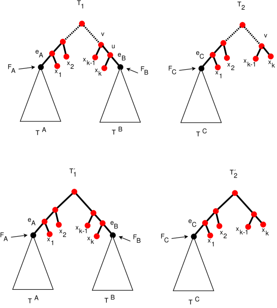
Figure 2: The situation when the common chain is pendant in exactly one tree.

Without loss of generality we assume that $K$ is pendant in $T_{2}$ and that the situation is as described in Figure 2. Let $f$ be an optimal character. Then we have the following two cases.

Case 1: In this first case $l_{f}(T_{1})<l_{f}(T_{2})$, so $d_{\textsc{MP}}(T_{1},T_{2})=l_{f}(T_{2})-l_{f}(T_{1})$. As in Equation (3) we have,

$$d_{\textsc{MP}}(T_{1},T_{2})=l_{f_{C}}(T^{C})-l_{f_{A}}(T^{A})-l_{f_{B}}(T^{B})+p.$$ (8)

In this case, $p\leq 1$ because of the usual mimicking construction (i.e. copying the states allocated to the red nodes in $T_{1}$, to $T_{2}$) used in the proof of Equation (4). That is, at most 1 extra mutation incurs in $T_{2}$ (i.e. on the edge $e_{C})$. On the other hand $p\geq 0$ follows from an argument similar to that for proving Equation (6). That is, we can always relabel $f$ to a new character $f^{*}=f[a,s,\ldots,s,b]$ where $a\in\mathbf{F}_{A}$, $b\in\mathbf{F}_{B}$ and $s$ is a state that does not appear elsewhere. This is either a $(2,2)$ or a $(2,3)$ situation, proving that $p\geq 0$. Hence, in Equation (8), we have $p\in\{0,1\}$, and hence it remains to prove that

$$d_{\textsc{MP}}(T^{\prime}_{1},T^{\prime}_{2})\geq l_{f_{C}}(T^{C})-l_{f_{A}}(T^{A})-l_{f_{B}}(T^{B})+p$$

holds, which will be done by considering the following two subcases.

1. $p=0$: Suppose first $\mathbf{F}_{A}\not\subseteq\mathbf{F}_{C}$. Let $a\in\mathbf{F}_{A}\setminus\mathbf{F}_{C}$. Note that $a\not\in\mathbf{F}_{B}$ because otherwise the character $f^{*}=f[a,a,...,a,a]$ would lead to a $(0,1)$ situation, contradicting $p=0$. This implies that the character $f^{\prime}=f[a,a,a,a]$ is a $(1,1)$ situation and we are done. So suppose next $\mathbf{F}_{A}\subseteq\mathbf{F}_{C}$. If $\mathbf{F}_{A}\cap\mathbf{F}_{B}\neq\emptyset$ then let $a\in\mathbf{F}_{A}\cap\mathbf{F}_{B}$. Clearly $a\in\mathbf{F}_{C}$. Taking character $f^{\prime}=f[a,a,a,a]$ yields a $(0,0)$ situation and we are done. Otherwise, $\mathbf{F}_{A}\cap\mathbf{F}_{B}=\emptyset$. In this situation, let $a\in\mathbf{F}_{A}\cap\mathbf{F}_{C}$ and let $b\in\mathbf{F}_{B}$. (Clearly, $a\neq b$). Consider character $f^{\prime}=f[a,a,b,b]$. This is a $(1,1)$ situation and we are done.

2. $p=1$: Suppose $\mathbf{F}_{A}\not\subseteq\mathbf{F}_{C}$. Let $a\in\mathbf{F}_{A}\setminus\mathbf{F}_{C}$. If $a\in\mathbf{F}_{B}$ then we take $f^{\prime}=f[a,a,a,a]$. This is a $(0,1)$ situation and we are done. If $a\not\in\mathbf{F}_{B}$, then let $b\neq a$ be an arbitrary element of $\mathbf{F}_{B}$. We take $f^{\prime}=f[a,a,b,b]$, this is a $(1,2)$ situation and we are done. The only subcase that remains is $\mathbf{F}_{A}\subseteq\mathbf{F}_{C}$, but this cannot happen by the less constrained roots argument.

Case 2: We have $l_{f}(T_{2})<l_{f}(T_{1})$, so $d_{\textsc{MP}}(T_{1},T_{2})=l_{f}(T_{1})-l_{f}(T_{2})$. In such a case we have

$$d_{\textsc{MP}}(T_{1},T_{2})=l_{f_{A}}(T^{A})+l_{f_{B}}(T^{B})-l_{f_{C}}(T^{C})+p.$$ (9)

We have $p\leq 2$, by the usual mimicking argument, but this time the red nodes in $T_{1}$ copy their states from $T_{2}$ and not the other way round. (Nodes $u$ and $x_{k}$ in $T_{1}$ should both be assigned the state that is assigned to $x_{k}$ in $T_{2}$). Also, $p\geq 1$ because we can relabel $f$ to a new character $f^{*}=f[s,s,\ldots,s,s]$ where $s$ is a state that does not appear elsewhere. This is a $(2,1)$ situation. Hence, $p\in\{1,2\}$. and hence it remains to prove that

$$d_{\textsc{MP}}(T^{\prime}_{1},T^{\prime}_{2})\geq l_{f_{A}}(T^{A})+l_{f_{B}}(T^{B})-l_{f_{C}}(T^{C})+p$$

holds, which will be done by considering the following two subcases.

1. $p=1$. Take $f^{\prime}=f[s,s,s,s]$, where $s$ is a state that does not appear elsewhere. This is a $(2,1)$ situation, and we are done.

2. $p=2$. Suppose $\mathbf{F}_{C}\not\subseteq\mathbf{F}_{A}$. Consider $f^{\prime}=f[c,c,s,s]$ where $s$ is a state that does not occur elsewhere and $c\in\mathbf{F}_{C}\setminus\mathbf{F}_{A}$. This is a $(3,1)$ situation and we are done. The only remaining case is $\mathbf{F}_{C}\subseteq\mathbf{F}_{A}$: but this is not possible by the less constrained roots argument.

III: Common chain is pendant in both trees

Figure 3: The situation when the common chain $K$ is pendant in both trees and the chain is oriented in the same direction in both trees (relative to the point of contact with the rest of the tree).

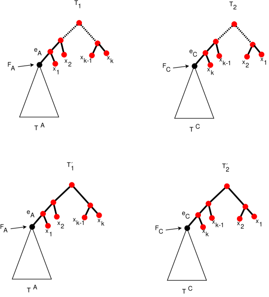
Figure 4: The situation when the common chain is pendant in both trees and the chain is oriented in different directions in the two trees (relative to the point of contact with the rest of the tree).

There are two main situations here: the chains are oriented in the same direction (Figure 3), and the chains are oriented in the opposite direction (Figure 4). Whichever situation occurs, we can assume without loss of generality that $l_{f}(T_{1})<l_{f}(T_{2})$, so $d_{\textsc{MP}}(T_{1},T_{2})=l_{f}(T_{2})-l_{f}(T_{1})$. As in Equation (3) we have,

$$d_{\textsc{MP}}(T_{1},T_{2})=l_{f_{C}}(T^{C})-l_{f_{A}}(T^{A})+p.$$ (10)

Note that we have $p\geq 0$ by the familiar trick of assigning all the taxa in $X(K)$ a state that does not occur elsewhere and $p\leq 1$ by the mimicking construction. It remains to show that

$$d_{\textsc{MP}}(T^{\prime}_{1},T^{\prime}_{2})\geq l_{f_{C}}(T^{C})-l_{f_{A}}(T^{A})+p$$

holds, which can be done by considering the following three cases:

Case 1: $p=0$. In this case we can just take $f^{\prime}=f[s,s,s,s]$ where $s$ is a state that does not appear elsewhere: this is a $(1,1)$ situation, and we are done.

Case 2: $p=1$ and we are in the same-direction situation. Observe that $\mathbf{F}_{A}\subseteq\mathbf{F}_{C}$ cannot hold by the less constrained roots argument. So $\mathbf{F}_{A}\not\subseteq\mathbf{F}_{C}$. Let $a\in\mathbf{F}_{A}\setminus\mathbf{F}_{C}$. Consider the character $f^{\prime}=f[a,s,s,s]$ where $s$ is a state that does not appear elsewhere. This is a $(1,2)$ situation and we are done.

Case 3: $p=1$ and we are in the opposite-direction situation. Then take $f^{\prime}=f[a,a,s,s]$ where $a\in\mathbf{F}_{A}$ and $s$ is a state that does not occur elsewhere. This is a $(1,2)$ situation (note that here we are exploiting the fact that $K$ is reversed in $T_{2}$ relative to $T_{1}$, the status of $\mathbf{F}_{C}$ is not relevant here), so we are done. ∎

Note that Theorem 3.1 is in some sense best possible, since reducing common chains to length 3 can potentially alter $d_{\textsc{MP}}$; see Figure 5 for a concrete example. Here $d_{\textsc{MP}}(T_{1},T_{2})\geq 2$ (due to character $abcdefgh=00001111$) and $d_{\textsc{MP}}(T_{1},T_{2})\leq d_{\textsc{TBR}}(T_{1},T_{2})\leq 2$ - due to the agreement forest $\{\{a,b\},\{c,d,e,f\},\{g,h\}\}$ - so $d_{\textsc{MP}}(T_{1},T_{2})=d_{\textsc{TBR}}(T_{1},T_{2})=2$. However, $d_{\textsc{MP}}(T^{\prime}_{1},T^{\prime}_{2})=1$ (achieved by character $abdefgh=0000111$); the fact that $d_{\textsc{MP}}(T^{\prime}_{1},T^{\prime}_{2})\leq 1$ can be verified computationally.

The chain reduction can easily be performed in polynomial time, and it can be applied at most a polynomial number of times because each application of the reduction reduces the number of taxa by at least 1. Hence, we obtain the following corollary.

Corollary 3.1.

Let $T_{1}$ and $T_{2}$ be two unrooted binary trees on the same set of taxa $X$. Then it is possible to transform $T_{1},T_{2}$ to $T^{\prime}_{1},T^{\prime}_{2}$ in polynomial time such that all common chains in $T^{\prime}_{1},T^{\prime}_{2}$ have length at most 4 and $d_{\textsc{MP}}(T_{1},T_{2})=d_{\textsc{MP}}(T^{\prime}_{1},T^{\prime}_{2})$.

Figure 5: Here $d_{\textsc{MP}}(T_{1},T_{2})=2$, while $d_{\textsc{MP}}(T^{\prime}_{1},T^{\prime}_{2})=1$. This shows that reducing common chains to length 3 does not preserve $d_{\textsc{MP}}$. Note that $d_{\textsc{TBR}}(T_{1},T_{2})=d_{\textsc{TBR}}(T^{\prime}_{1},T^{\prime}_{2})=2$, because $d_{\textsc{TBR}}$ is preserved under reduction of chains to length 3 [1].

4 A generalized subtree reduction

Let $T_{1}$ and $T_{2}$ be two unrooted binary trees on a set of taxa $X$. A split $A|B$ (on $X$) is simply a bipartition of $X$ i.e. $A\cap B=\emptyset$, $A\cup B=X$, $A,B\neq\emptyset$. For a phylogenetic tree $T$ on $X$, we say that edge $e$ induces a split $A|B$ if, after deleting $e$, $A$ is the subset of taxa appearing in one connected component and $B$ is the subset of taxa appearing in the other.

Figure 6: Here $T_{1}$ and $T_{2}$ have a common pendant subtree on $\{a,b,c\}$, and a common pendant subtree ignoring root location on $\{d,e,f,g\}$. Note that $T_{1}|_{\{d,e,f,g\}}=T_{2}|_{\{d,e,f,g\}}$ but the rooted variants $(T_{1}|_{\{d,e,f,g\}})^{\rho}$ and $(T_{2}|_{\{d,e,f,g\}})^{\rho}$ are not equal because they have different root locations (indicated here with an arrow).

Consider $X^{\prime}\subset X$. We say that $T_{1}$ and $T_{2}$ have a common pendant subtree ignoring root location (i.r.l.) on $X^{\prime}$ if (1) for $i\in\{1,2\}$, $T_{i}$ contains an edge $e_{i}=\{u_{i},v_{i}\}$ such that $e_{i}$ induces a split $(X\setminus X^{\prime})|X^{\prime}$ in $T_{i}$ and (2) $T_{1}|X^{\prime}=T_{2}|X^{\prime}$. Now, assume without loss of generality that for $i\in\{1,2\}$, $v_{i}$ is the endpoint of edge $e_{i}$ that is closest to taxon set $X^{\prime}$. The node $v_{i}$ can be used to “root” $T_{i}|_{X^{\prime}}$, yielding a rooted binary phylogenetic tree on $X^{\prime}$ which we denote $(T_{i}|_{X^{\prime}})^{\rho}$. If $T_{1}$ and $T_{2}$ have the additional property that $(T_{1}|_{X^{\prime}})^{\rho}=(T_{2}|_{X^{\prime}})^{\rho}$ (where here the equality operator is acting over rooted trees), then we say that $T_{1}$ and $T_{2}$ have a common pendant subtree on $X^{\prime}$. Clearly, a common pendant subtree on $X^{\prime}$ is also a common pendant subtree i.r.l. on $X^{\prime}$, but the other direction does not necessarily hold. The following reduction takes both types of subtrees into account.

Generalized subtree reduction: Let $T_{1}$ and $T_{2}$ be two unrooted binary trees on $X$. Let $X^{\prime}$ be a subset of $X$ such that $|X^{\prime}|\geq 2$. (If $T_{1}=T_{2}$ and $X^{\prime}=X$, then clearly $d_{\textsc{MP}}(T_{1},T_{2})=0$ so $T_{1}$ and $T_{2}$ can simply be replaced with a single taxon. We henceforth assume $X^{\prime}\subset X$). Suppose $T_{1}$ and $T_{2}$ have a common pendant subtree i.r.l. on $X^{\prime}$. We construct a reduced pair of trees $T^{\prime}_{1}$ and $T^{\prime}_{2}$ as follows. If $T_{1}$ and $T_{2}$ have a common pendant subtree on $X^{\prime}$, we are in the traditional case. If they do not, and $|X^{\prime}|\geq 4$, we are in the extended case. If we are in neither case, the generalized subtree reduction does not apply.

• Traditional case. Let $T^{\prime}_{1}=T_{1}|_{(X\setminus X^{\prime})\cup\{x\}}$ and $T^{\prime}_{2}=T_{2}|_{(X\setminus X^{\prime})\cup\{x\}}$ where $x\in X^{\prime}$. (This is the “traditional” subtree reduction, as described in e.g. [1] and [21].)

• Extended case. Without loss of generality let $x,y,z$ be distinct taxa in $X^{\prime}$ such that in $(T_{1}|_{X^{\prime}})^{\rho}$, $x$ and $y$ are on one side of the root, and $z$ on the other, while in $(T_{2}|_{X^{\prime}})^{\rho}$ $x$ and $z$ are on one side of the root, and $y$ on the other. These taxa always exist because $(T_{1}|_{X^{\prime}})^{\rho}\neq(T_{2}|_{X^{\prime}})^{\rho}$. We let $T^{\prime}_{1}=T_{1}|(X\setminus X^{\prime})\cup\{x,y,z\}$ and $T^{\prime}_{2}=T_{2}|(X\setminus X^{\prime})\cup\{x,y,z\}$.

Note that the reduction can easily be applied in polynomial time. Also, each application reduces the number of taxa by at least one, so if the reduction is applied repeatedly it will stop after at most polynomially many iterations.

Theorem 4.1.

Let $T_{1}$ and $T_{2}$ be two unrooted binary trees on the same set of taxa $X$. Suppose that $T^{\prime}_{1}$ and $T^{\prime}_{2}$ are two reduced trees obtained by applying the generalized subtree reduction to $T_{1}$ and $T_{2}$. Then $d_{\textsc{MP}}(T^{\prime}_{1},T^{\prime}_{2})=d_{\textsc{MP}}(T_{1},T_{2})$.

Proof.

If the traditional case applies, then the result is immediate from [21]. Hence, let us assume that we are in the extended case. As in the proof of Theorem 3.1, $d_{\textsc{MP}}(T^{\prime}_{1},T^{\prime}_{2})\leq d_{\textsc{MP}}(T_{1},T_{2})$ follows from Corollary 3.5 of [21]. It remains to show $d_{\textsc{MP}}(T^{\prime}_{1},T^{\prime}_{2})\geq d_{\textsc{MP}}(T_{1},T_{2})$. To this end, we may further assume $d_{\textsc{MP}}(T_{1},T_{2})>0$ as otherwise the theorem clearly holds.

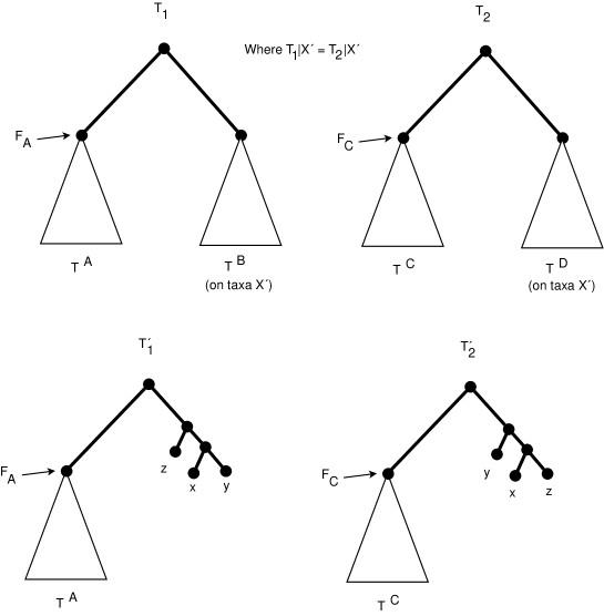
Figure 7: The generalized subtree reduction as it behaves in its extended case. That is, when $|X^{\prime}|\geq 4$, $T_{1}|_{X^{\prime}}=T_{2}|_{X^{\prime}}$ but $(T_{1}|_{X^{\prime}})^{\rho}\neq(T_{2}|_{X^{\prime}})^{\rho}$.

Let $f$ be an optimal character (in the usual sense) for $T_{1}$ and $T_{2}$ i.e. $|l_{f}(T_{1})-l_{f}(T_{2})|=d_{\textsc{MP}}(T_{1},T_{2})$. Let $T^{A},T^{B},T^{C},T^{D}$ refer to the 4 subtrees of $T_{1},T_{2}$ shown in Figure 7. For $P\in\{A,B,C,D\}$, let $X_{P}$ refer to the taxa in subtree $T^{P}$. Here $X_{B}=X_{D}=X^{\prime}$, $X_{A}=X_{C}=X\setminus X^{\prime}$ and $T_{1}|X^{\prime}=T_{2}|X^{\prime}$. That is, $T^{B}$ and $T^{D}$ are identical subtrees assuming we ignore the point at which each subtree is connected to the rest of its tree. As indicated in the figure, we root $T_{1}$ and $T_{2}$ (to put them in an appropriate form for Fitch-extensions) by subdividing the edge that connects each pendant subtree to the rest of the tree. Let $f_{P}$ denote the character obtained by restricting $f$ to $X_{P}$, and let $\mathbf{F}_{A}$ refer to the set of states assigned to the root of $T^{A}$ by the Fitch map induced by $f_{A}$.

For $i\in\{1,2\}$, let $m_{i}=0$ if the root of $T_{i}$ is an intersection node, and $m_{i}=1$ otherwise (i.e. the root is a union node). Then we have

$$l_{f}(T_{1}) =l_{f_{A}}(T^{A})+l_{f_{B}}(T^{B})+m_{1},~{}~{}~{}\mbox{and}$$

$$l_{f}(T_{2}) =l_{f_{C}}(T^{C})+l_{f_{D}}(T^{D})+m_{2}.$$

Note that we also have $l_{f_{B}}(T^{B})=l_{f_{D}}(T^{D})$ because $T^{B}$ and $T^{D}$ are (from an unrooted perspective) identical.

In the remainder of the proof we shall assume that $l_{f}(T_{1})<l_{f}(T_{2})$, as the other case $l_{f}(T_{1})>l_{f}(T_{2})$ is symmetrical. Let $p=m_{2}-m_{1}$. Then we have

$$d_{\textsc{MP}}(T_{1},T_{2}) =l_{f}(T_{2})-l_{f}(T_{1})$$

$$=(l_{f_{C}}(T^{C})+l_{f_{D}}(T^{D})+m_{2})-(l_{f_{A}}(T^{A})+l_{f_{B}}(T^{B})+m_{1})$$

$$=l_{f_{C}}(T^{C})-l_{f_{A}}(T^{A})+(m_{2}-m_{1})$$

$$=l_{f_{C}}(T^{C})-l_{f_{A}}(T^{A})+p.$$ (11)

Now we claim $p\in\{0,1\}$. To see this, by definition of $p$ it suffices to show that $p\geq 0$: Indeed, fix a state $s$ that is not used elsewhere and consider the character $f^{*}$ obtained from modifying $f$ by assigning all the taxa in $X^{\prime}$ to the state $s$; then we have $l_{f^{*}}(T_{2})=l_{f_{C}}(T^{C})+1$ and $l_{f^{*}}(T_{1})=l_{f_{A}}(T^{A})+1$, from which we can conclude that $d_{\textsc{MP}}(T_{1},T_{2})\geq l_{f^{*}}(T_{2})-l_{f^{*}}(T_{1})=l_{f_{C}}(T^{C})-l_{f_{A}}(T^{A})$, and hence $p\geq 0$.

In order to show $d_{\textsc{MP}}(T^{\prime}_{1},T^{\prime}_{2})\geq d_{\textsc{MP}}(T_{1},T_{2})$, by Equation (11) it suffices to show that

$$d_{\textsc{MP}}(T^{\prime}_{1},T^{\prime}_{2})\geq l_{f_{C}}(T^{C})-l_{f_{A}}(T^{A})+p.$$ (12)

To shorten notation we will write $f[a,b,c]$ to denote the character on $(X\setminus X^{\prime})\cup\{x,y,z\}$ obtained from $f$ by leaving the states assigned to taxa in $X_{A}=X_{C}=(X\setminus X^{\prime})$ intact and assigning states $a,b,c$ to $x,y,z$ respectively. Since $p\in\{0,1\}$, we have the following two cases:

Case 1: $p=0$. Let $f^{\prime}=f[s,s,s]$ where $s$ is a state that does not appear elsewhere. Then $l_{f^{\prime}}(T^{\prime}_{1})=l_{f_{A}}(T^{A})+1$ and $l_{f^{\prime}}(T^{\prime}_{2})=l_{f_{C}}(T^{C})+1$. This implies

$$d_{\textsc{MP}}(T^{\prime}_{1},T^{\prime}_{2})\geq l_{f^{\prime}}(T^{\prime}_{2})-l_{f^{\prime}}(T^{\prime}_{1})=l_{f_{C}}(T^{C})-l_{f_{A}}(T^{A}),$$

from which Equation (12) follows and we are done.

Case 2: $p=1$. Let $a\in\mathbf{F}_{A}$ and let $s$ be a state that does not appear elsewhere. Consider $f^{\prime}=f[s,s,a]$. Observe that $l_{f^{\prime}}(T^{\prime}_{1})=l_{f_{A}}(T^{A})+1$ and $l_{f^{\prime}}(T^{\prime}_{2})=l_{f_{C}}(T^{C})+2$, so we are done by an argument similar to that in Case 1. ∎

Note that the generalized subtree reduction could be used to replace the “pendant in both trees” case of the chain reduction. If the chains are oriented the same way they will be reduced to a single taxon (using the traditional case of the subtree reduction) and if they are oriented in opposite direction they will be reduced to a subtree of size 3 (using the extended case of the subtree reduction). We have described the chain reduction and the generalized subtree reduction separately to emphasize that in terms of correctness the two reductions are independent of each other.

5 Parameterized algorithms

As stated in the introduction, combining Theorems 4.1 and 3.1 with the kernelization in [1] and the exponential-time algorithm for $d_{\textsc{MP}}$ described in [18], yields the following theorem:

Theorem 1.1. Let $T_{1}$ and $T_{2}$ be two unrooted binary trees on the same set of species $X$. Computation of $d_{\textsc{MP}}(T_{1},T_{2})$ is fixed parameter tractable in parameter $d_{\textsc{TBR}}=d_{\textsc{TBR}}(T_{1},T_{2})$. More specifically, $d_{\textsc{MP}}(T_{1},T_{2})$ can be computed in time $O(\phi^{c\cdot d_{\textsc{TBR}}}\cdot\emph{poly}(|X|))$ where $\phi\approx 1.618...$ is the golden ratio and $c\leq 112/3$.

We close the main part of the paper by observing that a purely theoretical version of Theorem 1.1 can be obtained via Courcelle’s Theorem [10, 2]. A few further definitions are first necessary. Given an undirected graph $G=(V,E)$, a bag is simply a subset of $V$. A tree decomposition of $G$ consists of a tree $T_{G}=(V(T_{G}),E(T_{G}))$ where $V(T_{G})$ is a collection of bags such that the following holds: (1) every node of $V$ is in at least one bag; (2) for each edge $\{u,v\}\in E$, there exists some bag that contains both $u$ and $v$; (3) for each node $u\in V$, the bags that contain $u$ induce a connected subtree of $T_{G}$. The width of a tree decomposition is equal to the cardinality of its largest bag, minus 1. The treewidth of a graph $G$, denoted $tw(G)$, is equal to the minimum width, ranging over all possible tree decompositions of $G$ [3, 4]. A tree with at least one edge has treewidth 1. The display graph of two unrooted binary phylogenetic trees $T_{1}$ and $T_{2}$, both on the same set of taxa $X$, is the graph $D(T_{1},T_{2})$ obtained by identifying leaves that are labelled with the same taxon [7]. See Figure 8 for an example. A formal description of Monadic Second Order Logic (MSOL) is beyond the scope of this article; we refer to [20] for an introduction relevant to phylogenetics. Informally, it is a type of logic used to describe properties of graphs, in which both universal (“for all”) and existential (“there exists”) quantification are permitted over (subsets of) nodes and (subsets of) edges.

Figure 8: The display graph $D(T_{1},T_{2})$ obtained from the trees $T_{1}$ and $T_{2}$ shown in Figure 6. The treewidth of this graph is 3, and $d_{\textsc{MP}}(T_{1},T_{2})=d_{\textsc{TBR}}(T_{1},T_{2})=1$.

Remark 5.1.

Let $T_{1}$ and $T_{2}$ be two unrooted binary trees on the same set of species $X$. Via Monadic Second Order Logic (MSOL) it can be shown that computation of $d_{\textsc{MP}}(T_{1},T_{2})$ is possible in time $g(d_{\textsc{TBR}})\cdot\emph{poly}(|X|)$ where $d_{\textsc{TBR}}=d_{\textsc{TBR}}(T_{1},T_{2})$ and $g$ is some computable function that depends only on $d_{\textsc{TBR}}$.

We do not give explicit details of this alternative FPT proof since the argument is extremely indirect and does not in any sense lead to a practical algorithm: the function $g$ is astronomical. However, for completeness we sketch the overall idea. In [20] it is shown that computation of $d^{2}_{\mathrm{MP}}$ (the variant of $d_{\textsc{MP}}$ in which characters are restricted to at most 2 states) is FPT in parameter $d_{\textsc{TBR}}$. The core insight there is (i) the display graph $D(T_{1},T_{2})$ has treewidth bounded by a function of $d_{\textsc{TBR}}$ and (ii) Fitch’s algorithm can be modelled in a static fashion by guessing an optimal character and subsequently guessing the Fitch maps induced by that character in the two trees (including whether each node is a union or intersection node). This naturally requires that the internal nodes of the trees are partitioned into $O(2^{|\mathbf{C}|})$ subsets, where as usual $\mathbf{C}$ is the set of states used by the optimal character. From [5] it is known that there always exists an optimal character in which $|\mathbf{C}|\leq 7d_{\textsc{MP}}-5$. Now, there is a polynomial-time 3-approximation for computation of $d_{\textsc{TBR}}$ (see [8] for a recent overview), so running such an algorithm yields a value $t$ such that $d_{\textsc{TBR}}\leq t\leq 3d_{\textsc{TBR}}$. Combining with the fact that $d_{\textsc{MP}}\leq d_{\textsc{TBR}}$ [14, 21], it follows that $7t-5$ is an upper bound on the number of states required to encode an optimal character for $d_{\textsc{MP}}$. Also, $7t-5$ is clearly bounded by a function of $d_{\textsc{TBR}}$, which means that the resulting sentence of MSOL has a length that is bounded by a (admittedly highly exponential) function of $d_{\textsc{TBR}}$. The result then follows from the optimization variant of Courcelle’s Theorem known as EMS which is described by Arnborg et al. in [2].

6 Discussion and open problems

A major open question is whether the two reductions discussed in this article (the chain reduction and the generalized subtree reduction) are together sufficient to obtain a kernel for $d_{\textsc{MP}}$. That is, after applying the rules repeatedly until they can no longer be applied, is it true that the number of taxa in the resulting instance is bounded by some function of $d_{\textsc{MP}}$? If answered affirmatively, this would prove that computation of $d_{\textsc{MP}}$ is FPT in its most natural parameterization, namely $d_{\textsc{MP}}$ itself, which would mean that $d_{\textsc{MP}}$ can be computed in time $f(d_{\textsc{MP}})\cdot\text{poly}(|X|)$ for some computable function $f$ that depends only on $d_{\textsc{MP}}$.

Note that, if it can be shown that $d_{\textsc{TBR}}\leq g(d_{\textsc{MP}})$ for some function $g$ that depends only on $d_{\textsc{MP}}$, then the desired FPT result will follow automatically from Theorem 1.1. In [21] it is claimed that $d_{\textsc{TBR}}\leq 2d_{\textsc{MP}}$, and while the claim itself is not known to be false, the proof is incorrect. In fact, at the present time we do not know how to prove $d_{\textsc{TBR}}\leq g(d_{\textsc{MP}})$ for any $g(.)$, even when $g$ is extremely fast-growing. Relatedly, we do not even know how to compute $d_{\textsc{MP}}$ in time $O(|X|^{f(d_{\textsc{MP}})})$ for any computable function $f$ that only depends on $d_{\textsc{MP}}$. Running times of this latter form (which are algorithmically weaker results than FPT) are trivial for $d_{\textsc{TBR}}$ and most other tree distances.

This is intriguing because, although tree-pairs are known where $d_{\textsc{TBR}}=2d_{\textsc{MP}}$ (see e.g. Figure 5), empirical tests suggest that $d_{\textsc{MP}}$ and $d_{\textsc{TBR}}$ are in practice often extremely close. The following simple experiment highlights this. For each $n\in\{10,15,20,25\}$ and $t\in\{0.2n,0.4n,0.6n,0.8n\}$ we generated 500 tree pairs, where the first tree is generated uniformly at random from the space of unrooted binary trees on $n$ taxa, and the second tree is obtained from the first by randomly applying at most $t$ TBR moves. We computed $d_{\textsc{MP}}$ using the algorithm described in [18] and $d_{\textsc{TBR}}$ using an ad-hoc Integer Linear Programming (ILP) formulation. The ILP formulation is the running time bottleneck, limiting us to 25 taxa. For every $(n,t)$ parameter combination, at most 1 tree-pair was observed that had $d_{\textsc{MP}}=d_{\textsc{TBR}}-2$ (and this was the largest difference we observed). In Table 1, the first number is the $\%$ of the 500 tree pairs that had $d_{\textsc{MP}}=d_{\textsc{TBR}}$, and the second number is the $\%$ of the tree pairs where $d_{\textsc{MP}}\geq d_{\textsc{TBR}}-1$.

$n,t$	$0.2n$	$0.4n$	$0.6n$	$0.8n$
10	99.8, 100	96.2, 100	91.6, 100	89, 100
15	99.2, 100	96.4, 99.8	94, 100	87, 100
20	99.8, 100	97.6, 100	90.2, 99.8	87.4, 100
25	99.8, 100	96.2, 100	91, 99.8	77.9, 100

Table 1: Percentage of the 500 tree-pairs on $n$ taxa (and at most $t$ TBR moves apart) in which $d_{\textsc{MP}}=d_{\textsc{TBR}}$, and $d_{\textsc{MP}}\geq d_{\textsc{TBR}}-1$, respectively.

Despite these empirical observations there are some clues that $d_{\textsc{MP}}$ and $d_{\textsc{TBR}}$ might ultimately have a rather different combinatorial structure. Consider the following construction. In [19] it is shown, for every integer $k\geq 2$, how to construct a (rooted) tree-pair $T_{1},T_{2}$ such that $d_{\textsc{MP}}(T_{1},T_{2})=d_{\textsc{TBR}}(T_{1},T_{2})=4k$ and,

$$(\max_{f}l_{f}(T_{2})-l_{f}(T_{1}))\geq(\max_{f}l_{f}(T_{1})-l_{f}(T_{2}))+(k+1).$$

(As usual $f$ in this context ranges over all characters). Such tree-pairs are considered “asymmetric”. Fix an arbitrary constant $k\geq 2$ and let $T_{1},T_{2}$ be such a tree-pair, where $X$ denotes their set of taxa. Produce exact copies of $T_{1},T_{2}$ on a new set of taxa $X^{\prime}$, and call these trees $T^{\prime}_{1},T^{\prime}_{2}$. Connect $T_{1}$ and $T^{\prime}_{2}$ together at their roots by an edge - call this new tree $T_{1}:T^{\prime}_{2}$ - and do the same for $T^{\prime}_{1}$ and $T_{2}$ to obtain the new tree $T^{\prime}_{1}:T_{2}$. Both $T_{1}:T^{\prime}_{2}$ and $T^{\prime}_{1}:T_{2}$ are on taxa set $X\cup X^{\prime}$ and both have a common split $X|X^{\prime}$.

It is straightforward to show that, due to the fact that $T_{1}:T^{\prime}_{2}$ and $T^{\prime}_{1}:T_{2}$ have been constructed by joining asymmetric trees together in “antiphase”, the following holds:

$$d_{\textsc{MP}}(T_{1}:T^{\prime}_{2},T^{\prime}_{1}:T_{2}) \leq 4k+(4k-(k+1))+1$$

$$=7k.$$

On the other hand, it is not too difficult to show (using agreement forests) that

$$d_{\textsc{TBR}}(T_{1}:T^{\prime}_{2},T^{\prime}_{1}:T_{2})=8k.$$

Given that $k$ can be chosen arbitrarily, the difference between $7k$ and $8k$ can be made arbitrarily large. This emphasizes that $d_{\textsc{MP}}$ and $d_{\textsc{TBR}}$ behave rather differently with regard to common splits. It also shows that if a tree-pair $T_{1},T_{2}$ has a common split $P|Q$, $d_{\textsc{MP}}(T_{1},T_{2})$ can (at least in an additive sense) be arbitrarily smaller than $d_{\textsc{MP}}(T_{1}|P,T_{2}|P)+d_{\textsc{MP}}(T_{1}|Q,T_{2}|Q)$.

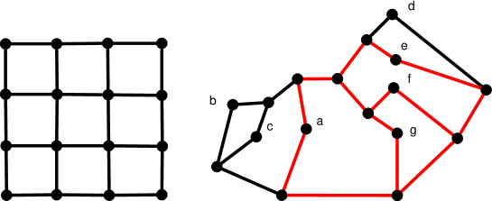
Figure 9: Left: a $4\times 4$ grid. Right: The red edges show the embedding of a $K_{4}$ minor (which is itself a minor of the $3\times 3$ grid) within the display graph $D(T_{1},T_{2})$ from Figure 8. The presence of this $K_{4}$ minor establishes that the treewidth of the display graph is at least 3, and thus $d_{\textsc{MP}}(T_{1},T_{2})>0$.

Computation of $d_{\textsc{MP}}$ also touches on a number of structural issues relevant to algorithmic graph theory. In the MSOL approach described in the previous section both the length of the logical sentence, and the treewidth of the display graph, are bounded by a function of $d_{\textsc{TBR}}$. It is natural to ask whether bounds in terms of $d_{\textsc{MP}}$, rather than $d_{\textsc{TBR}}$, could be obtained because this would prove that $d_{\textsc{MP}}$ is FPT in its most natural parameterization (independently of the exact relationship between $d_{\textsc{MP}}$ and $d_{\textsc{TBR}}$). To bound the length of the sentence by a function of $d_{\textsc{MP}}$ it will be necessary to identify a polynomial-time computable upper bound on $|\mathbf{C}|$ (the number of states used by some optimal character) that is bounded by a function of $d_{\textsc{MP}}$. This is a challenging question, albeit one that is tied closely to the very specific combinatorial structure of $d_{\textsc{MP}}$.

Establishing an $f(d_{\textsc{MP}})$ bound on the treewidth of the display graph (for some function $f$) is, however, fundamental, in the following sense. An undirected graph $H$ is a minor of an undirected graph $G$ if $H$ can be obtained from $G$ by deleting nodes, deleting edges and contracting edges [11]. The $n\times n$ grid graph is (as its name suggests) simply the graph on $n^{2}$ nodes corresponding to the $n\times n$ square grid (see Figure 9 for an example). From the grid minor theorem it is well-known that if a graph has treewidth $\geq k$, it has a grid minor of size at least $h(k)\times h(k)$ for a function $h$ that grows at least polylogarithmically quickly as a function of $k$ [23, 22] (for more recent, stronger bounds on $h$ see [9]). Hence, to prove that the treewidth of the display graph is bounded by some function of $d_{\textsc{MP}}$ it is sufficient to prove that, as grid minors in the display graph become larger and larger, $d_{\textsc{MP}}$ must also grow. The example of the $3\times 3$ grid minor is illustrative (see Figure 9). If the display graph contains a $3\times 3$ grid minor, it must also contain a $K_{4}$ minor (the complete undirected graph on 4 nodes), since $K_{4}$ is a minor of the $3\times 3$ grid. Two compatible (i.e. $d_{\textsc{MP}}=0$) phylogenetic trees induce display graphs of treewidth (at most) 2 [7, 16], and graphs of treewidth at most 2 are characterized by the absence of $K_{4}$ minors. Hence, the presence of a $3\times 3$ grid minor in the display graph implies $d_{\textsc{MP}}>0$.

Intuitively it seems plausible that larger grid minors will induce ever larger incongruencies between the two trees, thus driving $d_{\textsc{MP}}$ further up. However, as demonstrated in [16] formalizing such an intuition is a formidable task, since the embeddings of the minors can “weave” between the two trees in a difficult to analyse fashion. Indeed, this raises the question whether, and under which circumstances, the presence of (grid) minors in the display graph $D(T_{1},T_{2})$ can be translated into phylogenetic-topological statements about $T_{1}$ and $T_{2}$. This intersects with an emerging literature at the interface of algorithmic graph theory and phylogenetics (see e.g. [16, 20, 25] and references therein).

7 Acknowledgements

We thank Olivier Boes for helpful discussions. We also thank the editor and the two anonymous referees for their constructive suggestions. SK and TW acknowledge the support of London Mathematical Society grant SC7-1516-05.

References

- [1] B. Allen and M. Steel. Subtree transfer operations and their induced metrics on evolutionary trees. Annals of Combinatorics, 5(1):1–15, 2001.
- [2] S. Arnborg, J. Lagergren, and D. Seese. Easy problems for tree-decomposable graphs. Journal of Algorithms, 12:308 – 340, 1991.
- [3] H. L. Bodlaender. A tourist guide through treewidth. Acta cybernetica, 11(1-2):1, 1994.
- [4] H. L. Bodlaender and A. M. C. A. Koster. Treewidth computations I. Upper bounds. Information and Computation, 208(3):259–275, 2010.
- [5] O. Boes, M. Fischer, and S. Kelk. A linear bound on the number of states in optimal convex characters for maximum parsimony distance. IEEE/ACM Transactions on Computational Biology and Bioinformatics, 2016. To appear, arxiv preprint arXiv:1506.06404 [q-bio.PE].
- [6] M. Bordewich and C. Semple. Computing the hybridization number of two phylogenetic trees is fixed-parameter tractable. IEEE/ACM Transactions on Computational Biology and Bioinformatics, 4:458–466, 2007.
- [7] D. Bryant and J. Lagergren. Compatibility of unrooted phylogenetic trees is FPT. Theoretical computer science, 351(3):296–302, 2006.
- [8] J. Chen, J-H. Fan, and S-H. Sze. Parameterized and approximation algorithms for maximum agreement forest in multifurcating trees. Theoretical Computer Science, 562:496–512, 2015.
- [9] J. Chuzhoy. Excluded grid theorem: Improved and simplified. In Proceedings of the Forty-Seventh Annual ACM on Symposium on Theory of Computing (STOC 2015), pages 645–654. ACM, 2015.
- [10] B. Courcelle. The monadic second-order logic of graphs. I. Recognizable sets of finite graphs. Information and Computation, 85(1):12–75, 1990.
- [11] R. Diestel. Graph Theory. Springer-Verlag Berlin and Heidelberg GmbH & Company KG, 2010.
- [12] R. Downey and M. Fellows. Fundamentals of parameterized complexity, volume 4. Springer, 2013.
- [13] J. Felsenstein. Inferring Phylogenies. Sinauer Associates, Incorporated, 2004.
- [14] M. Fischer and S. Kelk. On the Maximum Parsimony distance between phylogenetic trees. Annals of Combinatorics, 20(1):87–113, 2016.
- [15] W. Fitch. Toward defining the course of evolution: minimum change for a specific tree topology. Systematic Zoology, 20(4):406–416, 1971.
- [16] A. Grigoriev, S. Kelk, and N. Lekić. On low treewidth graphs and supertrees. Journal of Graph Algorithms and Applications, 19(1):325, 2016.
- [17] G. Hickey, F. Dehne, A. Rau-Chaplin, and C. Blouin. SPR distance computation for unrooted trees. Evolutionary Bioinformatics Online, 4:17–27, 2008.
- [18] S. Kelk. A note on convex characters and Fibonacci numbers. arXiv preprint arXiv:1508.02598 [q-bio.PE], 2015. Submitted.
- [19] S. Kelk and M. Fischer. On the complexity of computing MP distance between binary phylogenetic trees. Annals of Combinatorics, 2016. To appear, arxiv preprint arXiv:1412.4076.
- [20] S. Kelk, L. J. J. van Iersel, C. Scornavacca, and M. Weller. Phylogenetic incongruence through the lens of monadic second order logic. Journal of Graph Algorithms and Applications, 20(2):189–215, 2016.
- [21] V. Moulton and T. Wu. A parsimony-based metric for phylogenetic trees. Advances in Applied Mathematics, 66:22–45, 2015.
- [22] N. Robertson, P. Seymour, and R. Thomas. Quickly excluding a planar graph. Journal of Combinatorial Theory, Series B, 62(2):323–348, 1994.
- [23] N. Robertson and P. D Seymour. Graph minors. V. Excluding a planar graph. Journal of Combinatorial Theory, Series B, 41(1):92–114, 1986.
- [24] M. Steel and D. Penny. Distributions of tree comparison metrics-some new results. Systematic Biology, pages 126–141, 1993.
- [25] S. Vakati and D. Fernández-Baca. Compatibility, incompatibility, tree-width, and forbidden phylogenetic minors. Electronic Notes in Discrete Mathematics, 50:337 – 342, 2015. LAGOS’15 – {VIII} Latin-American Algorithms, Graphs and Optimization Symposium.
- [26] C. Whidden, N. Zeh, and R. Beiko. Supertrees based on the Subtree Prune-and-Regraft distance. Systematic Biology, 63(4):566–581, 2014.
- [27] T. Wu, V. Moulton, and M. Steel. Refining phylogenetic trees given additional data: An algorithm based on parsimony. IEEE/ACM Transactions on Computational Biology and Bioinformatics, 6(1):118–125, 2009.
- [28] J. Yang, J. Li, L. Dong, and S. Grünewald. Analysis on the reconstruction accuracy of the Fitch method for inferring ancestral states. BMC Bioinformatics, 12(1):18, 2011.