The renormalized Hamiltonian truncation

method in the large $E_{T}$ expansion

J. Elias-Miró^a, M. Montull^b,, M. Riembau^b,c,
a  SISSA and INFN, I–34136 Trieste, Italy
^b  Institut de Física d’Altes Energies (IFAE), Barcelona Institute of Science
and Technology (BIST) Campus UAB, E-08193 Bellaterra, Spain
^c DESY, Notkestrasse 85, 22607 Hamburg, Germany

Hamiltonian Truncation Methods are a useful numerical tool to study strongly coupled QFTs. In this work we present a new method to compute the exact corrections, at any order, in the Hamiltonian Truncation approach presented by Rychkov et al. in Refs. [1, 2, 3]. The method is general but as an example we calculate the exact $g^{2}$ and some of the $g^{3}$ contributions for the $\phi^{4}$ theory in two dimensions. The coefficients of the local expansion calculated in Ref. [1] are shown to be given by phase space integrals. In addition we find new approximations to speed up the numerical calculations and implement them to compute the lowest energy levels at strong coupling. A simple diagrammatic representation of the corrections and various tests are also introduced.

1 Introduction and review

An outstanding problem in theoretical physics is to solve strongly coupled Quantum Field Theories (QFT). When they are not amenable to analytic calculations one can resort to numerical approaches. The two most used numerical approaches are lattice simulations and direct diagonalization of truncated Hamiltonians. In this paper we further develop the Hamiltonian truncation method recently presented in Ref. [1, 2, 3], that renormalizes the truncated Hamiltonian $H_{T}$ to improve the numerical accuracy.

The Hamiltonian truncation method consists in truncating the Hamiltonian $H$ into a large finite matrix $(H_{T})_{ij}$ and then diagonalizing it numerically. There is a systematic error with this approach that vanishes as the size of the truncated Hamiltonian $H_{T}$ is increased. There are different versions of the Hamiltonian truncation method that mainly differ on the frame of quantization and the choice of basis in which $H$ is truncated. Two broad categories within the Hamiltonian truncation methods are the Truncated Conformal Space Approach [4] and Discrete Light Cone Quantization [5]. A less traveled route consists in using the Fock-Space basis to truncate the Hamiltonian [6, 7, 8, 9, 10, 1, 2]. Lately there have been many advances in the Hamiltonian Truncation methods, see for instance [3, 11, 12, 13, 14, 15, 16, 17].

We review the truncated Hamiltonian approach following the discussion of Ref. [3, 1]. The problem we are interested in is finding the spectrum of a strongly coupled QFT. Therefore we want to solve the eigenvalue equation

$$H|\mathinner{{{\cal E}}\,\rangle}={\cal E}|\mathinner{{{\cal E}}\,\rangle}\,,$$ (1)

where $H=H_{0}+V$, $H_{0}$ is a solvable Hamiltonian or the free Hamiltonian and $V$ is the potential. $H_{0}$ is diagonalized by the states $H_{0}|\mathinner{{E_{n}}\,\rangle}=E_{n}|\mathinner{{E_{n}}\,\rangle}$. Suppose we are interested in studying the lowest energy states of the theory. One way to do it is separating the Hilbert space ${\cal H}$ into ${\cal H}={\cal H}_{l}\oplus{\cal H}_{h}$, where ${\cal H}_{l}$ is of finite dimension and it is spanned by the states $|\mathinner{{E_{n}}\,\rangle}$ with $E_{n}\leq E_{T}$. Then, the Hilbert space ${\cal H}_{h}$ is an infinite-dimensional Hilbert space containing the rest of the states $E_{n}>E_{T}$. The states are projected as $P_{l}|\mathinner{{x}\,\rangle}\equiv|\mathinner{{x_{l}}\,\rangle}\in{\cal H}_{l}$ and $(\mathds{I}-P_{l})|\mathinner{{x}\,\rangle}=P_{h}|\mathinner{{x}\,\rangle}\equiv|\mathinner{{x_{h}}\,\rangle}\in{\cal H}_{h}$. Then, the eigenvalue problem can be replaced by

$$H_{eff}({\cal E})|\mathinner{{{\cal E}_{l}}\,\rangle}={\cal E}|\mathinner{{{\cal E}_{l}}\,\rangle}\,,$$ (2)

where $H_{eff}\equiv H_{T}+\Delta H({\cal E})$, the truncated Hamiltonian is $H_{T}=P_{l}HP_{l}$ and

$$\Delta H({\cal E})=V_{lh}\frac{1}{{\cal E}-H_{0\,hh}-V_{hh}}V_{hl}\,,$$ (3)

with $O_{ij}\equiv P_{i}OP_{j}$ for $i,j\in\{h,l\}$. To derive Eq. (2), project Eq. (1) into the two equations

$$H_{ll}|\mathinner{{{\cal E}_{l}}\,\rangle}+H_{lh}|\mathinner{{{\cal E}_{h}}\,\rangle}={\cal E}|\mathinner{{{\cal E}_{l}}\,\rangle}\,,\quad\quad H_{hl}|\mathinner{{{\cal E}_{l}}\,\rangle}+H_{hh}|\mathinner{{{\cal E}_{h}}\,\rangle}={\cal E}|\mathinner{{{\cal E}_{h}}\,\rangle}\,,$$ (4)

and then substitute $|\mathinner{{{\cal E}_{h}}\,\rangle}=\left({\cal E}-H_{hh}\right)^{-1}H_{hl}|\mathinner{{{\cal E}_{l}}\,\rangle}$ from the second equation in (4) into the first.

Notice that Eq. (2) is an exact equation and that a complete knowledge of $\Delta H({\cal E})$ would render the original eigenvalue problem of Eq. (1) solvable by an easy numerical diagonalization. In the limit where $E_{T}\rightarrow\infty$ the corrections $\Delta H$ to $H_{T}$ can be neglected, but it is computationally very costly to increase the size of $H_{T}$ and then diagonalize it. Therefore it is interesting to calculate $\Delta H$ to improve the numerical accuracy for a given $E_{T}$. A first step to compute $\Delta H$ is to perform an expansion of Eq. (2) in powers of $V_{hh}({\cal E}-H_{0})^{-1}$,

$$\Delta H({\cal E},\,E_{T})=\sum_{n=0}^{\infty}\Delta H_{n}({\cal E},E_{T})\ ,\ \ \text{where}\quad\Delta H_{n}({\cal E},\,E_{T})=V_{lh}\frac{1}{{\cal E}-E_{hh}}\left(V_{hh}\frac{1}{{\cal E}-E_{hh}}\right)^{n}V_{hl}\,,$$

where the matrix elements of $\Delta H_{n}$ are given by

$$\Delta H_{n}({\cal E})_{rs} = \sum_{\begin{subarray}{c}j_{1},\cdots\,,j_{n}-1:\,E_{j_{i}}>E_{T}\end{subarray}}V_{rj_{1}}\frac{1}{{{\cal E}-E_{j_{1}}}}V_{j_{1}j_{2}}\frac{1}{{\cal E}-E_{j_{2}}}V_{j_{2}j_{3}}\cdots V_{j_{n-2}j_{n-1}}\frac{1}{{\cal E}-E_{j_{n-1}}}V_{j_{n-1}s}\,,\quad\quad$$ (5)

in the $H_{0}$ eigenbasis and the sums run over all labels $j_{1},\,\dots,\,j_{n-1}$ of states belonging to ${\cal H}_{h}$ with $r,s$ denoting the matrix elements (corresponding to eigenstates of $H_{0}$ with $E_{s},E_{r}\leq E_{T}$ eigenvalues). Naively the truncation of the series in Eq. (5) is justified for $V_{hh}/H_{0\,hh}<1$ which for large enough $E_{T}$ and ${\cal E}\ll E_{T}$ is fulfilled, and allows to go to strong coupling. This is discussed in detail in Sec. 5.3. The operator $\Delta H$ depends on the exact eigenvalue and in practice the way Eq. (2) is solved is by diagonalizing iteratively $H_{eff}({\cal E}^{*})$ starting with an initial seed ${\cal E}^{*}$. It is convenient to take ${\cal E}^{*}$ close to the exact eigenvalue ${\cal E}$, a simple and effective choice is to take the eigenvalue obtained from diagonalizing $H_{T}$.

In Ref. [1] the $\phi^{4}$ theory in two dimensions was studied at strong coupling using the Hamiltonian truncation method just presented in the Fock basis. There, the leading terms of $\Delta H_{2}$ doing a local expansion were computed and shown to improve the results with respect to the ones found by only diagonalizing $H_{T}$. The main result of our work is to explain a way to calculate the exact corrections to $\Delta H$ at any order $\Delta H_{n}$. As an example we calculate the $\Delta H_{2}$ correction and some of the $\Delta H_{3}$ terms for the $\phi^{4}$ theory in two dimensions and present various approximation schemes for a faster numerical implementation. This can be seen as an extension of the method presented in Ref. [1] which we believe to be very promising.

The paper is organized as follows. In Sec. 2 we introduce a general formula to compute $\Delta H_{n}({\cal E},\,E_{T})$ at any order $n$. Then we apply the method to the $\phi^{2}$ and $\phi^{4}$ scalar field theories in $d=2$ space-time dimensions which we first define in Sec. 3. The method is tested in Sec. 4 by studying the spectrum of the solvable $\phi^{2}$ perturbation with the calculation of $\Delta H_{2}$ and $\Delta H_{3}$. Other numerical tests are also performed in this section. Next, in Sec. 5 we give the $\Delta H_{2}$ correction for the $\phi^{4}$ theory, and discuss the $\Delta H_{3}$ calculation with some examples. There we also discuss the convergence of the $\Delta H_{n}$ expansion and compute the lowest energy levels of the theory at strong coupling. In Sec. 6, we conclude and outline future directions of the method that are left open. In Appendix A we introduce a simple diagrammatic representation to compute $\Delta H_{n}$. Lengthy derivations and results are relegated to the Appendices B and C. All the numerical calculations for this work have been done with Mathematica.

2 Calculation of $\Delta H$ at any order

In this section we present one of the main results of this paper which is the derivation of the $n$th-order correction $\Delta H_{n}$ of Eq. (5) to the Truncated Hamiltonian. We start by defining the operator

$$\Delta\widehat{H}({\cal E})=\sum_{n=2}^{\infty}\Delta\widehat{H}_{n}({\cal E})\,,\quad\text{where}\quad\Delta\widehat{H}_{n}({\cal E})=\left(V\frac{1}{{\cal E}-H_{0}}\right)^{n-1}V\,$$ (6)

which in the $H_{0}$ eigenbasis is given by

$$\Delta\widehat{H}_{n}({\cal E})_{rs} = \sum_{j_{1},\,\dots,\,j_{n-1}=1}^{\infty}V_{rj_{1}}\frac{1}{{{\cal E}-E_{j_{1}}}}V_{j_{1}j_{2}}\frac{1}{{\cal E}-E_{j_{2}}}V_{j_{2}j_{3}}\cdots V_{j_{n-2}j_{n-1}}\frac{1}{{\cal E}-E_{j_{n-1}}}V_{j_{n-1}s}\,,\quad\quad$$ (7)

where the indices $j_{1},\,j_{2},\,\dots\,,j_{n-1}$ run over the states of the full Hilbert space ${\cal H}$. Notice that the only difference between $\Delta H_{n}$ and $\Delta\widehat{H}_{n}$ is that the later receives contributions from all the eigenstates of $H_{0}$ while $\Delta H_{n}$ only from those with $E_{j}$ energies $E_{j}>E_{T}$. This translates into the fact that each term in $\Delta H_{n}({\cal E})$ has all the poles located at ${\cal E}>E_{T}$ as seen in Eq. (5).

From here the derivation of $\Delta H_{n}$ follows from the observation that Eq. (7) can be rewritten as the improper Fourier transform of the product of potentials restricted to positive times

$$\Delta\widehat{H}_{n}({\cal E})_{rs}=\lim_{\epsilon\rightarrow 0}\,(-i)^{n-1}\int_{0}^{\infty}dt_{1}\cdots dt_{n-1}\ e^{i({\cal E}-E_{r}+i\epsilon)(t_{1}+\cdots t_{n-1})}\,{\cal T}\left\{V\left(T_{1}\right)\cdots V\left(T_{n}\right)\right\}_{rs}\,,$$ (8)

where $T_{k}=\sum_{i=1}^{i=n-k}t_{i}$, $V(t)=e^{iH_{0}t}Ve^{-iH_{0}t}$ and ${\cal T}$ denotes the time ordering operation . Then, our method consists in applying the Wick theorem to Eq. (8) to calculate $\Delta\widehat{H}_{n}$ and obtaining $\Delta H_{n}$ by keeping only the terms of $\Delta\widehat{H}_{n}$ corresponding to states with $E_{j}>E_{T}$, i.e. by keeping only the terms of $\Delta\widehat{H}_{n}$ which have all poles above $E_{T}$.  In the following sections we show how to carry this procedure for the cases of the $\phi^{2}$ perturbation and $\phi^{4}$ theory.

3 Scalar theories

We study scalar theories in two space-time dimensions defined by the Minkowskian action $S=S_{0}+S_{I}$ where

$$S_{0}=\frac{1}{2}\int_{-\infty}^{\infty}dt\int_{0}^{L}dx\,:(\partial\phi)^{2}-m^{2}\phi^{2}:\,\,,$$ (9)

$$S_{I}=-\int_{-\infty}^{\infty}dt\,V(\phi)=-g_{\alpha}\int_{-\infty}^{\infty}dt\int_{0}^{L}dx\,:\phi^{\alpha}:\,.$$ (10)

For simplicity we consider the cases where $\alpha=2,\,4$ and $m^{2}>0$. The symbol $:\,:$ stands for normal ordering which for $S_{0}$ means that we set the vacuum energy to zero; while the interaction term is normal ordered with respect to $S_{0}$, which in perturbation theory is equivalent to renormalize to zero the UV divergences from closed loops with propagators starting and ending on the same vertex.

To study these theories using the Hamiltonian truncation method we begin by defining them on the cylinder $\mathbb{R}\times S_{1}$ where the circle corresponds to the space direction which we take to have a length $Lm\gg 1$, and $\mathbb{R}$ is the time. We impose periodic boundary conditions $\phi(t,x)=\phi(t,x+nL)$ for $n\in{\mathbb{Z}}$ on $S_{1}$. The compact space direction makes the spectrum of the free theory discrete and regularizes the infra-red (IR) divergences.

In canonical quantization the scalar operators can be expanded in terms of creation and annihilation operators as

$$\phi(x)=\sum_{k}\frac{1}{\sqrt{2L\omega_{k}}}\left(a_{k}e^{ikx}+a_{k}^{\dagger}e^{-ikx}\right)\,,$$ (11)

where $\omega_{k}=\sqrt{m^{2}+k^{2}}$, $k=\frac{2\pi n}{L}$ with $n\in\mathbb{Z}$ and the creation and anihilation operators satisfy the commutation relations

$$[a_{k},\,a_{k^{\prime}}^{\dagger}]=\delta_{kk^{\prime}}\,,\quad\quad[a_{k},\,a_{k^{\prime}}]=0\,.$$ (12)

The Hamiltonian then reads $H=H_{0}+V$, where

$$H_{0}=\sum_{k}\omega_{k}\,a_{k}^{\dagger}a_{k}$$ (13)

and the potentials for a $\phi^{2}$ and a $\phi^{4}$ interaction are given by

$$V=g_{2}\sum_{k_{1}k_{2}}\frac{L\,\delta_{k_{1}+k_{2},0}}{\sqrt{2L\omega_{k_{1}}}\sqrt{2L\omega_{k_{2}}}}\left(a_{k_{1}}a_{k_{2}}+a_{-k_{1}}^{\dagger}a_{k_{2}}\right)+h.c.\,,$$ (14)

and

$$V=g\sum_{k_{1},k_{2},k_{3},k_{4}}\frac{L\,\delta_{\sum_{i=1}^{4}k_{i},0}}{\prod_{i=1}^{4}\sqrt{2L\omega_{k_{i}}}}\left(a_{k_{1}}a_{k_{2}}a_{k_{3}}a_{k_{4}}+4a_{-k_{1}}^{\dagger}a_{k_{2}}a_{k_{3}}a_{k_{4}}+3a_{-k_{1}}^{\dagger}a_{-k_{2}}^{\dagger}a_{k_{3}}a_{k_{4}}\right)+h.c.\,,\quad$$ (15)

respectivley, where $g\equiv g_{4}$ and $\delta_{k_{1}+k_{2},0}$, $\delta_{\sum_{i=1}^{4}k_{i},0}$ stand for Kronecker deltas.

We implement the Hamiltonian truncation using the basis of $H_{0}$ eigenstates

$$|\mathinner{{E_{i}}\,\rangle}=\frac{a^{\dagger\,n_{N}}_{k_{N}}}{\sqrt{n_{N}!}}\cdots\frac{a^{\dagger\,n_{2}}_{k_{2}}}{\sqrt{n_{2}!}}\frac{a^{\dagger\,n_{1}}_{k_{1}}}{\sqrt{n_{1}!}}|\mathinner{{0}\,\rangle}\,.$$ (16)

which satisfy $\mathds{I}=\sum_{i}|\mathinner{{E_{i}}\,\rangle}\mathinner{\langle{E_{i}}}|$, where $E_{i}=\sum_{s=1}^{N}n_{s}\sqrt{k_{s}^{2}+m^{2}}$ and $H_{0}|\mathinner{{0}\,\rangle}=0$ . The Hilbert space is divided into ${\cal H}={\cal H}_{l}\oplus{\cal H}_{h}$ with ${\cal H}_{l}$ spanned by the states $|\mathinner{{E_{r}}\,\rangle}$ such that $E_{i}\leq E_{T}$ while ${\cal H}_{h}$ is spanned by the rest of the basis. Then, the truncated Hamiltonian is

$$(H_{T})_{rs}=\mathinner{\langle{E_{r}}}|H|\mathinner{{E_{s}}\,\rangle}\,,\quad\text{for}\quad E_{i}\leq E_{T}\,.$$ (17)

In this basis, the operator $\Delta H$ is given by

$$\Delta H({\cal E})_{rs}=\sum_{j,\,j^{\prime}}V_{rj}\,\Big{(}\frac{1}{{\cal E}-H_{0}-V}\Big{)}_{jj^{\prime}}\,V_{j^{\prime}s}\,$$ (18)

where the labels $r,\,s$ denote entries with $E_{r},E_{s}\leq E_{T}$ and the sum over $j,\,j^{\prime}$ runs over all states with $E_{j},E_{j^{\prime}}>E_{T}$.

The Hamiltonian $H$ can be diagonalized by sectors with given quantum numbers associated with operators that commute with $H$. These are the total momentum $P$, the spatial parity ${\cal P}:x\rightarrow-x$ and the field parity $\mathds{Z}_{2}:\,\phi(x)\rightarrow-\phi(x)$, which act on the $H_{0}$-eigenstates as $P|\mathinner{{E_{i}}\,\rangle}=\sum_{s}n_{s}k_{s}|\mathinner{{E_{i}}\,\rangle}$, ${\cal P}\prod_{i=1}^{N}\frac{a^{\dagger\,n_{i}}_{k_{i}}}{\sqrt{n_{i}!}}|\mathinner{{0}\,\rangle}=\prod_{i=1}^{N}\frac{a^{\dagger\,n_{i}}_{-k_{i}}}{\sqrt{n_{i}!}}|\mathinner{{0}\,\rangle}$ and $\mathds{Z}_{2}|\mathinner{{E_{i}}\,\rangle}=(-1)^{\sum_{s}n_{s}}|\mathinner{{E_{i}}\,\rangle}$. We work in the orthonormal basis of eigenstates of $H_{0}$, $P$, $\cal P$ and $\mathds{Z}_{2}$ given by

$$|\mathinner{{\widetilde{E}_{i}}\,\rangle}=\beta\cdot\left(|\mathinner{{E_{i}}\,\rangle}+{\cal P}\,|\mathinner{{E_{i}}\,\rangle}\right)\,,$$ (19)

where $\beta=1/2$, $1/\sqrt{2}$ for ${\cal P}\,|\mathinner{{E_{i}}\,\rangle}=|\mathinner{{E_{i}}\,\rangle}$ and ${\cal P}\,|\mathinner{{E_{j}}\,\rangle}\neq|\mathinner{{E_{j}}\,\rangle}$, respectively. As done in Ref. [1], in the whole paper we focus on the sub-sector with total momentum $P|\mathinner{{\widetilde{E}_{i}}\,\rangle}=0$, spatial parity ${\cal P}|\mathinner{{\widetilde{E}_{i}}\,\rangle}=+|\mathinner{{\widetilde{E}_{i}}\,\rangle}$ and diagonalize separately the $\mathds{Z}_{2}=\pm$ sectors.  In this paper we do not investigate the dependence of the spectrum as a function of the length $L$ of the compact dimension which we leave for future work, and always consider it to be finite.  All the numerical calculations are done for $m=1$ and $L=10$.

4 Case study $\mbox{\boldmath{$\phi$}}^{2}$ perturbation

In this section we apply the method introduced in Sec. 2 to the scalar theory $H=H_{0}+V$ with a potential

$$V=g_{2}\int_{0}^{L}dt\,:\phi^{2}:$$ (20)

This is a simple theory that allows to illustrate various aspects of the calculation of $\Delta\widehat{H}$ in Eq. (8) and its relation to $\Delta H$. Also since the theory is solvable we can compare our procedure with the exact results. The theory is solved by using the eigenstates of $H$, given by

$$|\mathinner{{{\cal E}_{i}}\,\rangle}=\frac{b^{\dagger\,n_{N}}_{k_{N}}}{\sqrt{n_{N}!}}\cdots\frac{b^{\dagger\,n_{2}}_{k_{2}}}{\sqrt{n_{2}!}}\frac{b^{\dagger\,n_{1}}_{k_{1}}}{\sqrt{n_{1}!}}|\mathinner{{\Omega}\,\rangle}\,,$$ (21)

where $|\mathinner{{\Omega}\,\rangle}=|\mathinner{{{\cal E}_{0}}\,\rangle}$ is the vacuum of the theory and $b^{\dagger}$/$b$ are the creation/annihilation operators so that

$$H=\sum_{k}b^{\dagger}_{k}b_{k}\Omega_{k}+{\cal E}_{0}\,,$$ (22)

with $\Omega_{k}=\sqrt{\omega^{2}_{k}+2g_{2}}$. Then, one can relate the operators $b^{\dagger}/b$ to the $a^{\dagger}/a$ in $H_{0}$ (given in Eq. (13) and Eq. (14)) by the Bogolyubov transformation $b_{k}=\sinh\alpha_{k}\,a_{-k}^{\dagger}+\cosh\alpha_{k}\,a_{k}$ provided that $\Omega_{k}\sinh 2\alpha_{k}=\omega_{k}^{-1}\,g_{2}$, $\Omega_{k}\cosh 2\alpha_{k}=\omega_{k}+g_{2}/\omega_{k}$. Then, since $\mathinner{\langle{0}}|H|\mathinner{{0}\,\rangle}=0$ we have that [1]:

$${\cal E}_{0}(g_{2})=\frac{1}{2}\sum_{k}\big{(}\sqrt{\omega_{k}^{2}+2g_{2}}-\omega_{k}-\frac{g_{2}}{\omega_{k}}\big{)}=\frac{L\left(m^{2}+2g_{2}\right)}{8\pi}\Big{[}\log\Big{(}\frac{m^{2}}{m^{2}+2g_{2}}\Big{)}+\frac{2g_{2}}{m^{2}+2g_{2}}\Big{]}\,,$$ (23)

where the sum can be done by means of the Abel-Plana formula, which is the exact vacuum energy of the theory.

A brief summary of the rest of this section is the following. In Sec. 4.1 and Sec. 4.2 we calculate the $2$ and $3$-point corrections to the operator $\Delta H$. In Sec. 4.3 we perform a numerical test to check that our expressions for $\Delta H$ are correct. Then, in Sec. 4.4 we discuss the numerical results and the convergence of the expansion $\Delta H({\cal E}_{i})=\sum_{n}\Delta H_{n}({\cal E}_{i})$ by comparing with the exact spectrum ${\cal E}_{i}$.

4.1 Two-point correction

Following the steps explained in Sec. 2 we begin the calculation of the two-point correction by first computing $\Delta\widehat{H}_{2}$. From Eq. (8) we have that

$$\Delta\widehat{H}_{2}({\cal E})_{rs}=\sum_{j}V_{rj}\frac{1}{{\cal E}-E_{j}}V_{js}=\lim_{\epsilon\rightarrow 0}-i\int_{0}^{\infty}dt\,e^{i({\cal E}-E_{r}+i\epsilon)t}{\cal T}\left\{V(t)V(0)\right\}_{rs}\,.$$ (24)

Then, applying the Wick theorem to Eq. (24) we find

$$\lim_{\epsilon\rightarrow 0}\,-ig_{2}^{2}\int_{0}^{\infty}dt\,e^{i({\cal E}-E_{r}+i\epsilon)t}\int_{-L/2}^{L/2}dxdz\,\sum_{m=0}^{2}s_{2-m}D_{F}^{2-m}(z,t):\phi^{m}(x+z,t)\phi^{m}(x,0):_{rs}\,,$$ (25)

where $s_{p}=\binom{2}{p}^{2}p!$ are the symmetry factors and $D_{F}(z,t)$ is the Feynman propagator with discretized momenta. Henceforth we label the terms $m=0,1,2$ by $\Delta\widehat{H}^{\phi^{2m}}_{2}$ so that $\Delta\widehat{H}_{2}=\Delta\widehat{H}^{\mathds{1}}_{2}+\Delta\widehat{H}^{\phi^{2}}_{2}+\Delta\widehat{H}^{\phi^{4}}_{2}$ and similarly for $\Delta H_{2}$; the labels only inform about the total number of fields in each term which do not need to be local. Due to the time integration domain, it is convenient to use half Feynman propagator

$$D_{L}(z,t)\equiv D_{F}(z,t)\theta(t)=\frac{1}{2L}\sum_{n=-\infty}^{n={\infty}}\frac{1}{\omega_{k}}e^{-i\omega_{k}t}e^{i\frac{2\pi nz}{L}}\theta(t)\,,$$ (26)

the momentum of the propagator is discretised due to the finite extent of the space. Next, we proceed to calculate the operators in Eq. (25), starting with the detailed calculation of the coefficient of the identity operator $\Delta\widehat{H}_{2}^{\mathds{1}}$:

$$\Delta\widehat{H}_{2}^{\mathds{1}}({\cal E})_{rs}=\lim_{\epsilon\rightarrow 0}\,-is_{2}g_{2}^{2}\int_{0}^{\infty}dt\int_{-L/2}^{L/2}dz\ e^{i({\cal E}-E_{r}+i\epsilon)t_{1}}D_{L}^{2}(t,z)\,\mathds{1}_{rs}\,,$$ (27)

where $\mathds{1}_{rs}\equiv\delta_{rs}\int_{-L/2}^{L/2}dz$ has dimensions of $[E]^{-1}$. Then, upon inserting the propagator of Eq. (26) and performing the space-time integrals we find

$$\Delta\widehat{H}_{2}^{\mathds{1}}({\cal E})_{rs}=\frac{s_{2}g_{2}^{2}}{4L}\sum_{k}\frac{1}{\omega_{k}^{2}}\frac{1}{{\cal E}-E_{r}-2\omega_{k}}\,\mathds{1}_{rs}\,.$$ (28)

The operator in Eq. (28) has poles from all possible intermediate states and, as explained in Sec. 2, the operator $\Delta H_{2}^{\mathds{1}}({\cal E})$ is found by keeping only those terms with poles located at $E_{r}+2\omega_{k}>E_{T}$, therefore

$$\Delta H_{2}^{\mathds{1}}({\cal E})_{rs} = \frac{s_{2}g_{2}^{2}}{L}\sum_{k:\,E_{r}+2\omega_{k}>E_{T}}\frac{1}{4\,\omega_{k}^{2}}\frac{1}{{\cal E}-E_{r}-2\omega_{k}}\,\mathds{1}_{rs}\ \,.$$ (29)

The calculations of $\Delta H_{2}^{\phi^{2}}$ is similar to the one for Eq. (29), we start by computing

$$\Delta\widehat{H}_{2}^{\phi^{2}}({\cal E})_{rs}=\lim_{\epsilon\rightarrow 0}\,-is_{1}g_{2}^{2}\int_{0}^{\infty}dt\int_{-L/2}^{L/2}dxdz\ e^{i({\cal E}-E_{r}+i\epsilon)t_{1}}D_{L}(z,t)\,:\phi(x+z,t)\phi(x,0):_{rs}\,,$$ (30)

where we expand $:\phi(x+z,t)\phi(x,0):$ in modes, as in Eq. (11), and do the simple space-time integrals. For the full expressions of $\Delta\widehat{H}_{2}^{\phi^{2}}$ see Appendix B. Then, keeping only the terms with poles at ${\cal E}>E_{T}$ we get

$$\Delta H_{2}^{\phi^{2}}({\cal E})_{rs}=s_{1}g_{2}^{2}\sum_{q:\,2\omega_{q}+E_{r}>E_{T}}\frac{1}{4\,\omega_{q}^{2}}\frac{1}{{\cal E}-E_{r}-2\omega_{q}}(a_{q}^{\dagger}a_{q})_{rs}\,.$$ (31)

The operator $\Delta H_{2}^{\phi^{4}}$ is obtained in a similar way,

$$\Delta H_{2}^{\phi^{4}}({\cal E})_{rs}=s_{0}g_{2}^{2}\sum_{q_{1},q_{2}:\,2\omega_{q_{2}}+E_{r}>E_{T}}\frac{1}{4\,\omega_{q_{2}}\omega_{q_{1}}}\frac{1}{{\cal E}-E_{r}-2\omega_{q_{2}}}\left(a_{q_{1}}^{\dagger}a_{-{q_{1}}}^{\dagger}a_{q_{2}}a_{-{q_{2}}}\right)_{rs}\,.$$ (32)

In Appendix A we give a simple way to derive these expressions from diagrams, and for the full expressions of $\Delta\widehat{H}_{2}^{\phi^{2}}$ and $\Delta\widehat{H}_{2}^{\phi^{4}}$ see Appendix B. Notice that the values of $q_{1}$, $q_{2}$ and $q$ appearing in the sums of Eq. (31) and Eq. (32) can take only the momenta of the states $|\mathinner{{E_{s}}\,\rangle}\in{\cal H}_{l}$ on which $a$ and $a^{\dagger}$ act, and therefore are bounded. On the other hand, the values of the $k$’s in Eq. (29) go all the way to infinity. Also, even though the operators in Eq. (31) and Eq. (32) may seem not hermitian due to the $E_{r}$ appearing in the expressions, one can see that the operator $(\Delta H_{2}^{\phi^{2}})_{rs}$ is diagonal and therefore $E_{r}=E_{s}$, while $\Delta H_{2}^{\phi^{4}}$ is not diagonal, but one can check that $E_{r}+2\omega_{q_{2}}=E_{s}+2\omega_{q_{1}}$, making it hermitian as well.

We end this section by noticing that the operator of Eq. (29) can be rewritten as

$$(\Delta H_{2}^{\mathds{1}})_{rs}=\int_{E_{T}}^{\infty}\frac{dE}{{\cal E}-E}\frac{s_{2}g_{2}^{2}}{L}\sum_{k=-\infty}^{\infty}\frac{\delta(E-E_{r}-2\omega_{k})}{(2\omega_{k})^{2}}\,\mathds{1}_{rs}=s_{2}g_{2}^{2}\int_{E_{T}}^{\infty}\frac{dE}{2\pi}\frac{\Phi_{2}(E-E_{r})}{{\cal E}-E}\,\mathds{1}_{rs}\,,$$ (33)

where $\Phi_{2}$ is the two-particle phase space with discretized momenta,

$$\Phi_{2}(E-E_{r})=\sum_{k_{1},k_{2}}\frac{L\,\delta_{k_{1}+k_{2},\,0}}{(2L\omega_{k_{1}})\,(2L\omega_{k_{2}})}\,2\pi\,\delta(E-E_{r}-\omega_{k_{1}}-\omega_{k_{2}})\,,$$ (34)

where from Eq. (33) one has that $E-E_{r}>2m$.  Eq. (33) can be evaluated by means of the Abel-Plana formula, which for $LE_{T}\gg 1$ is well approximated by its continuum limit . The continuum two-body phase space is given by

$$\Phi_{2}(E)=\int_{-\infty}^{\infty}\frac{d^{2}p_{1}}{(2\pi)^{2}\,2\omega_{p_{1}}}\frac{d^{2}p_{2}}{(2\pi)^{2}\,2\omega_{p_{2}}}\,(2\pi)^{2}\,\delta^{(2)}(P^{\mu}-p_{1}-p_{2})=\frac{1}{E\sqrt{E^{2}-4m^{2}}}\,,$$ (35)

where $P^{\mu}=(E,0)$ and $E>2m$. Therefore (for $LE_{T}\gg 1$) we find

$$\Delta H_{2}^{\mathds{1}}({\cal E})_{rs}\simeq s_{2}g_{2}^{2}\int_{E_{T}}^{\infty}\frac{dE}{2\pi}\frac{1}{{\cal E}-E}\frac{1}{E-E_{r}}\frac{1}{\sqrt{(E-E_{r})^{2}-4m^{2}}}\,\theta(E-E_{r}-2m)\,\mathds{1}_{rs}\,.$$ (36)

This result is useful for numerical implementation since Eq. (36) can be integrated in terms of logarithmic functions. Finally, we notice that upon expanding the function $s_{2}/(2\pi)\Phi_{2}(E)$ around $m/E=0$ we find agreement with Ref. [1] that computed it by other means (there called $\mu_{220}(E)=1/(\pi E^{2})$).

4.2 Three-point correction

The calculation of the three-point correction $\Delta H_{3}$ also starts from the expression in Eq. (8)

$$\Delta\widehat{H}_{3}({\cal E})_{rs}=-\lim_{\epsilon\rightarrow 0}\int_{0}^{\infty}dt_{1}dt_{2}\,e^{i({\cal E}-E_{r}+i\epsilon)(t_{1}+t_{2})}{\cal T}\left\{V(T_{1})V(T_{2})V(T_{3})\right\}_{rs}\,,$$ (37)

where $T_{k}=\sum_{n=1}^{3-k}t_{n}$. Next we apply the Wick theorem and find that the time ordered product ${\cal T}\left\{V(T_{1})V(T_{2})V(T_{3})\right\}$ is given by

$$g_{2}^{3}\int_{-L/2}^{L/2}dx_{1}dx_{2}dz\sum_{m,n,v=0}^{2}s^{mnv}_{2}D_{F}^{m}(x_{1},t_{1})D_{F}^{n}(x_{2},t_{2})D_{F}^{v}(x_{1}+x_{2},t_{1}+t_{2}):\phi^{2-n-m}_{X_{1},T_{1}}\phi^{2-n-v}_{X_{2},T_{2}}\phi^{2-v-m}_{X_{3},T_{3}}:$$ (38)

where we have introduced the notation $X_{k}=z+\sum_{n=1}^{3-k}x_{n}$ and $\phi_{x,t}=\phi(x,t)$; while the symmetry factor is given by

$$s^{mnv}_{p}=\frac{p!^{3}}{(p-m-n)!(p-m-v)!(p-n-v)!m!n!v!}\,.$$ (39)

We use the same notation as in the previous section $\Delta\widehat{H}_{3}=\Delta\widehat{H}^{\mathds{1}}_{3}+\Delta\widehat{H}^{\phi^{2}}_{3}+\Delta\widehat{H}^{\phi^{4}}_{3}+\Delta\widehat{H}^{\phi^{6}}_{3}$, and similarly for $\Delta H_{3}$. Then, upon performing the space-time integrals in Eq. (38) and only keeping the terms with all the poles above $E_{T}$ we find $\Delta H_{3}$. Then, for the term $\Delta H_{3}^{\mathds{1}}$ we get

$$\Delta H_{3}^{\mathds{1}}({\cal E})_{rs}=s_{2}^{111}g_{2}^{3}\frac{1}{L}\sum_{k:E_{rs}+2\omega_{k}>E_{T}}\frac{1}{(2\omega_{k})^{3}}\frac{1}{\left({\cal E}-E_{r}-2\omega_{k}\right)^{2}}\,\mathds{1}_{rs}\,.$$ (40)

The expressions for $\Delta H_{3}^{\phi^{2}}$, $\Delta H_{3}^{\phi^{4}}$ and $\Delta H_{3}^{\phi^{6}}$ are lengthy but straightforward to obtain and are relegated to Appendix B.

As done in the previous section, Eq. (40) can be written as

$$\Delta H_{3}^{\mathds{1}}({\cal E})_{rs}=s_{2}^{111}g_{2}^{3}\int_{E_{T}}^{\infty}\frac{dE}{({\cal E}-E)^{2}}\frac{1}{L}\sum_{k}\frac{1}{(2\omega_{k})^{3}}\delta(E-E_{r}-2\omega_{k})\,\mathds{1}_{rs}\,,$$ (41)

which for $L^{-1}E_{T}\gg 1$ is well approximated by its continuum limit

$$\Delta H_{3}^{\mathds{1}}({\cal E})_{rs}\simeq s_{2}^{111}\,\frac{g_{2}^{3}}{2\pi}\int_{E_{T}}^{\infty}\frac{dE}{({\cal E}-E)^{2}}\frac{1}{(E-E_{r})^{2}}\frac{1}{\sqrt{(E-E_{r})^{2}-4m^{2}}}\,\mathds{1}_{rs}\,,$$ (42)

and can be integrated in terms of logarithmic functions. This is useful for a fast numerical implementation.

4.3 A numerical test

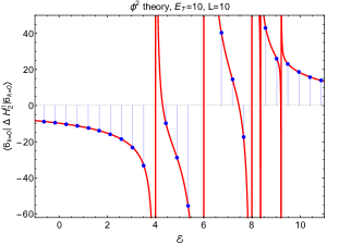
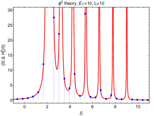
Figure 1: Comparison of both sides of Eqs. (43) and (44).

We perform a numerical check to test our prescription to select the poles of $\Delta\widehat{H}_{n}({\cal E})$ to get $\Delta H_{n}$, i.e. that we can select the desired intermediate states of $H_{0}$ by looking at the poles of the terms of $\Delta\widehat{H}_{n}$. The check consists in computing $\Delta\widehat{H}_{2}$ as explained, and then selecting only the terms with all poles at ${\cal E}\leq E_{T}$. We refer to the expression as $\Delta H^{ll}_{n}$ to differentiate it with $\Delta H_{n}$ that only receives corrections from terms with poles at ${\cal E}>E_{T}$. $\Delta H^{ll}_{2}$ is then compared with the matrix elements of $VP_{l}({\cal E}-H_{0})^{-1}P_{l}V$, finding an exact agreement. The same is done for $\Delta\widehat{H}_{3}({\cal E})$ by comparing it against $VP_{l}({\cal E}-H_{0})^{-1}V({\cal E}-H_{0})^{-1}P_{l}V$. This check has been done for all the matrices used in the present work, both for $\phi^{2}$ and $\phi^{4}$. For brevity we only show the check for two matrix entries of the $\phi^{2}$ theory. These are

$$\mathinner{\langle{6_{k=0}}}|\,VP_{l}\frac{1}{{\cal E}-H_{0}}P_{l}V|\mathinner{{6_{k=0}}\,\rangle} = \sum_{k:\,2\omega_{k}+6m<E_{T}}\frac{g_{2}^{2}}{2\,\omega_{k}^{2}}\frac{1}{{\cal E}-6m-2\omega_{k}}$$ (43)

$$+ \frac{3\,g_{2}^{2}}{2m^{2}}\left(\frac{5}{{\cal E}-4m}+\frac{24}{{\cal E}-6m}+\frac{9}{{\cal E}-8m}\right),$$

$$\mathinner{\langle{0}}|\,VP_{l}\frac{1}{{\cal E}-H_{0}}V\frac{1}{{\cal E}-H_{0}}P_{l}V\,|\mathinner{{0}\,\rangle} = g_{2}^{3}\sum_{k:\,2\omega_{k}<E_{T}}\frac{1}{\omega_{k}^{3}}\frac{1}{({\cal E}-2\omega_{k})^{2}}\,.$$ (44)

In Fig. 1 we compare both sides of equations Eq. (43) and (44). The red curves correspond to the right hand side of Eqs. (43)-(44), which are our analytical results, and the blue dots are given by the product of the matrices in the left hand side of the equations. In the left plot, done for $\mathinner{\langle{6_{k=0}}}|\Delta H^{ll}_{2}|\mathinner{{6_{k=0}}\,\rangle}$, the first pole arises at the four-particle threshold and subsequent poles appear for higher excited states. Instead, the first pole in the right plot, done for $\mathinner{\langle{0}}|\Delta H^{ll}_{3}|\mathinner{{0}\,\rangle}$, occurs at ${\cal E}=2m$. Notice that in both figures there are no poles for ${\cal E}>E_{T}$.

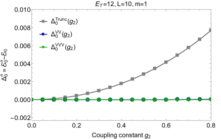
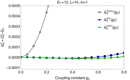
Figure 2: Left: comparison of the exact vacuum energy with the numerical result as a function of the coupling constant $g_{2}$ (for $V=g_{2}\int dx\phi^{2}$). Right: left plot with the $y$-axis zoomed in a factor $\times 20$.

4.4 Spectrum and convergence

We perform a numerical study of the convergence of the energy levels as a function of the truncation energy $E_{T}$ and their convergence as higher order corrections $\Delta H_{n}$ are calculated for a fixed $E_{T}$. We use the formulas in Eqs. (29)-(32), (40) and (B.5)-(B.8) to numerically compute $\Delta H_{2}$ and $\Delta H_{3}$. 

We begin by comparing the vacuum eigenstate ${\cal E}_{0}^{i}$ obtained by numerically diagonalizing $H_{T}+\sum_{n=2}^{N}\Delta H_{n}$ (for $N=2$ and 3) with the exact vacuum energy ${\cal E}_{0}$. In Fig. 2 we show a plot of $\Delta_{0}^{i}={\cal E}_{0}^{i}-{\cal E}_{0}$ as a function of the coupling constant $g_{2}$. The plot is done for a truncation energy of $E_{T}=12$ and $L=10$ (recall that we work in $m=1$ units). For an easier comparison with previous work, these plots have been done with the same choice of parameters and normalizations as in Fig. 2 of Ref. [1]. The gray curve in Fig. 2 is obtained by numerically diagonalizing $H_{T}$, whose lowest eigenvalue is ${\cal E}_{0}^{\text{T}}$. The blue curve is obtained by diagonalizing the renormalized hamiltonian $H_{T}+\Delta H_{2}({\cal E}_{0}^{\text{T}})$, whose lowest eigenvalue is ${\cal E}_{0}^{VV}$. Lastly, the green curve is obtained by diagonalizing $H_{T}+\Delta H_{2}({\cal E}_{0}^{VV})+\Delta H_{3}({\cal E}_{0}^{VV})$ (we find little difference in evaluating the latter operator in ${\cal E}_{0}^{\text{Trunc}}$ instead of ${\cal E}_{0}^{VV}$). The right plot of Fig. 2 is a zoomed in version of the left plot in order to resolve the difference between the $\Delta_{0}^{VV}$ and $\Delta_{0}^{VVV}$ curves.

The right plot shows that overall $\Delta_{0}^{VVV}$ performs better than $\Delta_{0}^{VV}$, this indicates that the truncation of the series expansion $\Delta H=\sum_{n=2}^{\infty}\Delta H_{n}$ at $n=3$ is perturbative in the studied range. The effect is more pronounced for the highest couplings $g_{2}\simeq[0.6,0.8]$. As a benchmark value ${\cal E}_{0}(g_{2}=0.8)=-0.351864$, see Eq. (23). Therefore the relative error at $g_{2}=0.8$ is $2\%$, $0.01\%$ and $0.002\%$ for the Truncated, the $VV$ and the $VVV$ corrections, respectively.

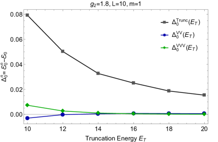
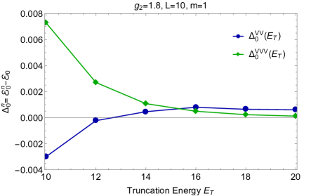
Figure 3: Left: comparison of the exact vacuum energy with the numerical result as a function of the truncation energy $E_{T}$. Right: left plot zoomed in.

Next, we check the convergence of the energy levels as a function of the truncation energy $E_{T}$. In Fig. 3, in the left plot we show $\Delta_{0}^{i}={\cal E}_{0}^{i}-{\cal E}_{0}$ as a function of the truncation energy $E_{T}$, for $i=$Trunc, $VV$ and $VVV$. Both the $\Delta_{0}^{VV}$ and $\Delta_{0}^{VVV}$ curves give better results than $\Delta_{0}^{\text{Trunc}}$ for the whole range. Also, the curves $\Delta_{0}^{VV}$ and $\Delta_{0}^{VVV}$ have a better convergence behavior and, when converged, they are closer to zero than $\Delta_{0}^{\text{Trunc}}$. The right plot is a zoomed in version to resolve the difference between $\Delta_{0}^{VV}$ and $\Delta_{0}^{VVV}$. The plot shows that for $E_{T}\lesssim 15$ the curve $\Delta_{0}^{VV}$ gives better results than $\Delta_{0}^{VVV}$ while for larger $E_{T}$ the behavior is reversed. This indicates that for $E_{T}\lesssim 15$ (and $g_{2}=1.8$) the truncation of the series $\Delta H=\sum_{n=2}^{\infty}\Delta H_{n}$ is not a good approximation, and adding more terms will not improve the accuracy. However, as $E_{T}$ is increased it pays off to introduce higher order corrections to get a better result. This is because $\Delta_{0}^{VVV}$ has a faster converge rate than $\Delta_{0}^{VV}$ to the real eigenvalue. The value is ${\cal E}_{0}(g_{2}=1.8)=-1.360719$, see Eq. (23). Therefore the relative error at $E_{T}=20$ is $1\%$, $0.04\%$ and $0.009\%$ for the Truncated, the $VV$ and the $VVV$ corrections, respectively.

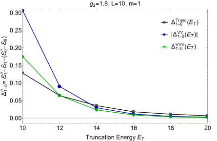
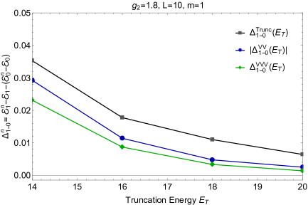
Figure 4: Left: comparison of the exact energy difference ${\cal E}_{1}-{\cal E}_{0}$ with respect the numerical result as a function of the truncation energy $E_{T}$. Right: left plot zoomed in. On both plots we have taken the absolute value of the curve corresponding to the $VV$ corrections, in blue.

In Fig. 4 we repeat the plots of Fig. 3 for the first $\mathds{Z}_{2}$-even excited state but taking the absolute value of the $\Delta_{1}^{VV}$ curve for clarity. The plots show a similar convergence rate for the three $\Delta_{1}^{i}$ curves. However, there is a similar pattern compared to Fig. 3: for $E_{T}\lesssim 15$ introducing higher order corrections of the series $\Delta H=\sum_{n=2}^{\infty}\Delta H_{n}$ gives worse results, while for larger values of $E_{T}$ adding higher $\Delta H_{n}$ corrections improves them. The value is ${\cal E}_{1}(g_{2}=1.8)=0.784042$, hence the relative error at $E_{T}=20$ is $0.8\%$, $0.3\%$ and $0.17\%$ for the Truncated, the $VV$ and the $VVV$ corrections, respectively.

5 The $\mbox{\boldmath{$\phi$}}^{4}$ theory

Next we apply the method presented in previous sections to the $\phi^{4}$ theory. We start by deriving the exact expressions for $\Delta H_{2}$ in detail, then we perform various useful approximations for a faster numerical implementation and discuss general aspects of the method. We also discuss the pertubativity of the $\Delta H_{n}$ expansion and compute the spectrum of the theory at different couplings while studying its behaviour in $E_{T}$ and $g$ using the results of $\Delta H_{2}$. We end the section with some comments on future work and a discussion of the calculation of $\Delta H_{3}$.

5.1 Two-point correction

Again, we follow Sec. 2 to derive $\Delta H$ by first computing $\Delta\widehat{H}$. From Eq. (8) we have

$$\Delta\widehat{H}_{2}({\cal E})_{rs}=\sum_{j}V_{rj}\frac{1}{{\cal E}-E_{j}}V_{js}=\lim_{\epsilon\rightarrow 0}-i\int_{0}^{\infty}dt\,e^{i({\cal E}-E_{r}+i\epsilon)t}{\cal T}\left\{V(t)V(0)\right\}_{rs}\,.$$ (45)

It is convenient to re-write the two-point correction in the following equivalent form

$$\Delta\widehat{H}_{2}({\cal E})_{rs}=\sum_{j}V_{rj}\frac{1}{{\cal E}-E_{j}}V_{js}=\lim_{\epsilon\rightarrow 0}-i\int_{0}^{\infty}dt\,e^{i({\cal E}-E_{rs}+i\epsilon)t}{\cal T}\left\{V(t/2)V(-t/2)\right\}_{rs}\,,$$ (46)

where $E_{rs}=(E_{r}+E_{s})/2$. Applying the Wick theorem we find

$$-ig^{2}\int_{0}^{\infty}dt\,e^{i({\cal E}-E_{rs}+i\epsilon)t}\int_{-L/2}^{L/2}dxdz\,\sum_{m=0}^{4}s_{4-m}D_{F}^{4-m}(z,t):\phi^{m}(x+z,t/2)\phi^{m}(x,-t/2):_{rs}\,,$$ (47)

where $s_{p}=\binom{4}{p}^{2}p!$ are the symmetry factors. By integrating Eq. (47) and keeping only the contributions from high energy intermediate states $E_{j}>E_{T}$ we obtain the exact expression for $\Delta H_{2}$. We use the shorthand notation $\Delta H_{2}=\Delta H^{\mathds{1}}_{2}+\Delta H^{\phi^{2}}_{2}+\Delta H^{\phi^{4}}_{2}+\Delta H^{\phi^{6}}_{2}+\Delta H^{\phi^{8}}_{2}$ for $m=0,1,2,3,4$, and similarly for $\Delta\widehat{H}_{2}$. For $\Delta H^{\mathds{1}}_{2}$, $\Delta H^{\phi^{2}}_{2}$ we obtain:

$$\Delta H_{2}^{\mathds{1}}({\cal E},E_{T}) = \frac{s_{4}g^{2}}{2^{4}L^{2}}\sum_{k_{1}k_{2}k_{3}k_{4}}\frac{1}{\omega_{k_{1}}\omega_{k_{2}}\omega_{k_{3}}\omega_{k_{4}}}F_{0}(k_{1},k_{2},k_{3},k_{4},{\cal E},E_{T})\,,$$ (48)

$$\Delta H_{2}^{\phi^{2}}({\cal E},E_{T}) = \frac{s_{3}g^{2}}{2^{4}L^{2}}\sum_{k_{1},k_{2},k_{3}}\sum_{q_{1},q_{2}}\,\frac{1}{\omega_{k_{1}}\omega_{k_{2}}\omega_{k_{3}}}\frac{1}{\sqrt{\omega_{q_{1}}\omega_{q_{2}}}}F_{2}(k_{1},k_{2},k_{3},q_{1},q_{2},{\cal E},E_{T})\,,$$ (49)

where $F_{0}(k_{1},k_{2},k_{3},k_{4},{\cal E},E_{T})$ is given by

$$F_{0\,rs}=\delta_{\Sigma_{i=1}^{4}k_{i},0}\,\frac{\theta(\omega_{k_{1}}+\omega_{k_{2}}+\omega_{k_{3}}+\omega_{k_{4}}+E_{rs}-E_{T})}{{\cal E}-\omega_{k_{1}}-\omega_{k_{2}}-\omega_{k_{3}}-\omega_{k_{4}}-E_{rs}}\,\mathds{1}_{rs}\,,$$ (50)

and the operator $F_{2}(k_{1},k_{2},k_{3},q_{1},q_{2},{\cal E},E_{T})$ is given by

$$F_{2\,rs} = \delta_{k_{1}+k_{2}+k_{3},q_{1}}\,\delta_{q_{1},-q_{2}}\frac{\theta(E_{rs}+\omega_{k_{1}}+\omega_{k_{2}}+\omega_{k_{3}}-E_{T})}{{\cal E}-E_{rs}-\omega_{k_{1}}-\omega_{k_{2}}-\omega_{k_{3}}}\,(a_{q_{1}}a_{q_{2}})_{rs}$$ (51)

$$+ \delta_{k_{1}+k_{2}+k_{3},q_{1}}\,\delta_{q_{1},-q_{2}}\frac{\theta(E_{rs}+\omega_{k_{1}}+\omega_{k_{2}}+\omega_{k_{3}}-E_{T})}{{\cal E}-E_{rs}-\omega_{k_{1}}-\omega_{k_{2}}-\omega_{k_{3}}}\,(a^{\dagger}_{q_{1}}a^{\dagger}_{q_{2}})_{rs}$$

$$+ \delta_{k_{1}+k_{2}+k_{3},q_{2}}\,\delta_{q_{1},q_{2}}\frac{\theta(E_{rs}+\omega_{k_{1}}+\omega_{k_{2}}+\omega_{k_{3}}+\omega_{q}-E_{T})}{{\cal E}-E_{rs}-\omega_{k_{1}}-\omega_{k_{2}}-\omega_{k_{3}}-\omega_{q}}\,(a^{\dagger}_{q_{1}}a_{q_{2}})_{rs}$$

$$+ \delta_{k_{1}+k_{2}+k_{3},q_{2}}\,\delta_{q_{1},q_{2}}\frac{\theta(E_{rs}+\omega_{k_{1}}+\omega_{k_{2}}+\omega_{k_{3}}-\omega_{q}-E_{T})}{{\cal E}-E_{rs}-\omega_{k_{1}}-\omega_{k_{2}}-\omega_{k_{3}}+\omega_{q}}\,(a^{\dagger}_{q_{1}}a_{q_{2}})_{rs}\,.\quad\quad\,$$

In Eqs. (48)-(49), all $q_{i}$’s are bounded from above ($q_{i}\leq q_{max}$) because they correspond to the momenta of creation/annihilation operators that act on the light states (i.e. states in ${\cal H}_{l}$). Instead the $k_{i}=2\pi n_{i}/L$ run over all possible values $n_{i}\in\mathbb{Z}$. Similar expressions for $\Delta H^{\phi^{4}}_{2},\,\Delta H^{\phi^{6}}_{2},\,\Delta H^{\phi^{8}}_{2}$ are given in Appendix C. As mentioned before, a simple way to derive these expressions from diagrams is given in Appendix A. We have performed the same kind of numerical checks done in Sec. 4.3 for all the operators $\Delta\widehat{H}_{2}$ in the $\phi^{4}$ theory.

Approximations

The exact expressions for $\Delta H_{2}$ are computationally demanding. Here we present different approximations that speed up the calculations and simplify their analytic structure. These basically consist in approximating the contribution from the highest energy states to $\Delta H$ in terms of a local expansion (as normally done in Effective Field Theory calculations), while keeping the contributions from lower energy states in their original non-local form. This is achieved by defining an energy $E_{L}$ and then by separating $\Delta H_{2}$ into two parts, $\Delta H_{2\,+}$ where we only sum over intermediate states with $E_{j}\geq E_{L}$ and $\Delta H_{2\,-}$ where we sum over those with $E_{T}<E_{j}<E_{L}$.

$$\Delta H_{2\,+}({\cal E},E_{L})_{rs} = \Delta H_{2}({\cal E},E_{L})_{rs},,$$ (52)

$$\Delta H_{2\,-}({\cal E},E_{T},E_{L})_{rs} = \Delta H_{2}({\cal E},E_{T})_{rs}-\Delta H_{2}({\cal E},E_{L})_{rs}\,.$$ (53)

We choose $E_{L}\gg E_{T}$ so that $\Delta H_{2\,+}$ is well approximated by local operators . As an example we show how to implement this procedure for the contribution of $\Delta H_{2}^{\phi^{2}}$ given in Eq. (49) and Eq. (51). We start by examining the term $\Delta H_{2\,+}^{\phi^{2}}({\cal E},E_{L})=\Delta H_{2}^{\phi^{2}}({\cal E},E_{L})$, which is obtained by replacing $E_{T}$ by $E_{L}$ in Eq. (51). In this case $\sum_{i}\omega_{k_{i}}\gtrsim E_{L}\gg E_{T}\gtrsim\omega_{q},E_{rs}$, and then it can be well approximated by

$$\Delta H_{2\,+}^{\phi^{2}}\simeq c_{2}\,V_{2}$$ (54)

with

$$c_{2}({\cal E},E_{L})=\frac{s_{3}g^{2}}{(2L)^{3}}\sum_{k_{1},k_{2},k_{3}}\frac{L\,\delta_{k_{1}+k_{2}+k_{3},0}}{\omega_{k_{1}}\omega_{k_{2}}\omega_{k_{3}}}\,\frac{\theta(\omega_{k_{1}}+\omega_{k_{2}}+\omega_{k_{3}}-E_{L})}{{\cal E}-\omega_{k_{1}}-\omega_{k_{2}}-\omega_{k_{3}}}\,,$$ (55)

and $V_{2}=\int_{0}^{L}dx\,\phi^{2}(x)$ which has dimensions of $[E]^{-1}$. The approximation in Eq. (54) receives corrections of at most ${\cal O}(E_{T}/E_{L})$. The expansion of $\Delta H_{2+}^{\phi^{2}}$ in terms of local operators can be obtained by expanding the term $\Delta\widehat{H}^{\phi^{2}}_{2}$ in Eq. (47) around $t,z=0$

$$\Delta\widehat{H}_{2}^{\phi^{2}}({\cal E})_{rs}=-ig^{2}s_{2}\int_{0}^{\infty}dt\,e^{i({\cal E}-E_{rs}+i\epsilon)t}\int_{-L/2}^{L/2}dzD_{F}^{2}(z,t)\int_{-L/2}^{L/2}dx\left[:\phi^{2}(x,0):_{rs}+{\cal O}(t^{2},z^{2})\,\right],$$ (56)

and, after integrating, keeping only the contributions from those states that produce poles at ${\cal E}>E_{L}$, when $E_{rs}$ is neglected. On the other hand $\Delta H_{2\,-}^{\phi^{2}}({\cal E},E_{T},E_{L})=\Delta H_{2}^{\phi^{2}}({\cal E},E_{T})-\Delta H_{2}^{\phi^{2}}({\cal E},E_{L})$ is given by the same expressions as in Eq. (49) and Eq. (51) but now the sums to perform are much smaller since the momenta of the intermediate states are restricted between $E_{T}$ and $E_{L}$.

The same exercise done for $\Delta H_{2+}^{\phi^{2}}$ can be done for $\Delta H^{\mathds{1}}_{2+}$ and $\Delta H^{\phi^{4}}_{2+}$ and one has that in the limit $E_{L}\gg E_{T}$

$$\Delta H_{2\,+}^{\mathds{1}}\simeq c_{0}\,\mathds{1}\,\,,\quad\quad\Delta H_{2\,+}^{\phi^{2}}\simeq c_{2}\,V_{2}\,\,,\quad\quad\Delta H_{2\,+}^{\phi^{4}}\simeq c_{4}\,V_{4}\,,$$ (57)

where $V_{\alpha}=\int_{0}^{L}dx\,\phi^{\alpha}(x)$ and has dimensions of $[E]^{-1}$,

$$c_{0}({\cal E},E_{L}) = \frac{s_{4}g^{2}}{(2L)^{4}}\sum_{k_{1},k_{2},k_{3},k_{4}}\frac{L\,\delta_{k_{1}+k_{2}+k_{3}+k_{4},0}}{\omega_{k_{1}}\omega_{k_{2}}\omega_{k_{3}}\omega_{k_{4}}}\,\frac{\theta(\omega_{k_{1}}+\omega_{k_{2}}+\omega_{k_{3}}+\omega_{k_{4}}-E_{L})}{{\cal E}-\omega_{k_{1}}-\omega_{k_{2}}-\omega_{k_{3}}-\omega_{k_{4}}}\,,$$ (58)

$$c_{4}({\cal E},E_{L}) = \frac{s_{2}g^{2}}{(2L)^{2}}\sum_{k_{1},k_{2}}\frac{L\,\delta_{k_{1}+k_{2},0}}{\omega_{k_{1}}\omega_{k_{2}}}\,\frac{\theta(\omega_{k_{1}}+\omega_{k_{2}}-E_{L})}{{\cal E}-\omega_{k_{1}}-\omega_{k_{2}}}\,,$$ (59)

and $c_{2}$ is given in Eq. (55). On the other hand the operators $\Delta H_{2}^{\phi^{6}}$ and $\Delta H_{2}^{\phi^{8}}$ are of the tree-level and disconnected type because they involve one and zero propagators respectively, see Eq. (47). Therefore the operators $\Delta H_{2+}^{\phi^{6}}$ and $\Delta H_{2+}^{\phi^{8}}$ are not well approximated by a local expansion, and we do not approximate them. For $E_{L}$ sufficiently big though, $\Delta H_{2+}^{\phi^{6}}=\Delta H_{2+}^{\phi^{8}}=0$ and all the contribution to $\Delta H_{2}^{\phi^{6}}$, $\Delta H_{2}^{\phi^{8}}$ comes from $\Delta H_{2-}^{\phi^{6}}$, $\Delta H_{2-}^{\phi^{8}}$, as can be explicitly seen from Eqs. (C.4)-(C.5). Notice that these operators only contribute to the entries of $\Delta H_{rs}$ with high values for $E_{r}$, $E_{s}$. Again, the coefficients of the local operators in Eq. (57) can be obtained by expanding $\Delta\widehat{H}_{2}$ in Eq. (47) around $t,z=0$

$$\Delta\widehat{H}_{2}({\cal E})_{rs}=-ig^{2}\int_{0}^{\infty}dt\,e^{i({\cal E}-E_{rs}+i\epsilon)t}\int_{-L/2}^{L/2}dxdz\,\sum_{m=0}^{4}s_{4-m}D_{F}^{4-m}(z,t):\phi^{2m}(x,0):_{rs}+{\cal O}(t,z)^{2}\,,$$ (60)

and, after integrating, keeping only the contributions from those states that produce poles at ${\cal E}>E_{L}$, when $E_{rs}$ is neglected. The evaluation of the coefficients in Eq. (57) can still be hard to evaluate numerically. In the next section we explain an alternative and simpler derivation of the coefficients $c_{2m}$ and further approximations to evaluate them.

5.2 Local expansion and the phase-space functions

From the first term in the local expansion of Eq. (60) the coefficients of the local operators are given by:

$$\hat{c}_{2n}({\cal E})=-ig^{2}s_{4-n}\int_{0}^{\infty}dte^{i({\cal E}+i\epsilon)t}\int_{-\infty}^{\infty}\,dx\,D_{F}^{4-n}(x,t)\,,$$ (61)

where $s_{4-n}$ is the symmetry factor and, as explained above, the common $E_{rs}$-shift on the eigenvalue ${\cal E}$ is neglected.  Next, applying the Kramers-Kronig dispersion relation to $c_{n}({\cal E})$ in Eq. (61)

$$\hat{c}_{2n}({\cal E})=-\int_{-\infty}^{\infty}\frac{dE}{\pi}\frac{1}{{\cal E}-E+i\epsilon}\text{Im}\,\hat{c}_{2n}({\cal E})\,.$$ (62)

Next, we compute $\text{Im }\hat{c}_{2n}$. First we do the space integral which, up to $g^{2}s_{4-n}$, yields

$$\text{Im}-i\sum_{k^{\prime}s}\frac{L\,\delta_{\sum_{i}k_{i},\,0}}{\prod_{i}2L\omega_{k_{i}}}\int_{0}^{\infty}dte^{i(E-\sum_{i}\omega_{k_{i}}+i\epsilon)t}=-\frac{1}{2}\sum_{k^{\prime}s}\frac{L\,\delta_{\sum_{i}k_{i},\,0}}{\prod_{i}2L\omega_{k_{i}}}\,2\pi\delta\Big{(}E-\sum_{i}\omega_{k_{i}}\Big{)}\,,$$ (63)

where we have used $D_{F}(t,x)\theta(t)=D(t,x)\theta(t)$ with $D(t,x)=\sum_{k}(2L\omega_{k})^{-1}e^{ikx-i\omega_{k}t}$. Therefore we find ,

$$\hat{c}_{2n}({\cal E})=\frac{g^{2}s_{4-n}}{2\pi}\int_{-\infty}^{\infty}\frac{dE}{{\cal E}-E+i\epsilon}\Phi_{{4-n}}(E)$$ (64)

where $\Phi_{m}(E)$ is the $m$-particle phase space

$$\Phi_{m}(E)=\sum_{k_{1},k_{2},\dots,k_{m}}\frac{L\,\delta_{\sum_{i=1}^{m}k_{i},\,0}}{\prod_{i=1}^{m}2L\omega_{k_{i}}}\,2\pi\delta\Big{(}E-\sum_{i=1}^{m}\omega_{k_{i}}\Big{)}\,.$$ (65)

Finally, the coefficients in Eq. (57) are obtained by including only the contributions from poles located at ${\cal E}\geq E_{L}$

$$c_{0}({\cal E}) = s_{4}\,g^{2}\ \int_{E_{L}}^{\infty}\frac{dE}{2\pi}\,\frac{1}{{\cal E}-E}\,\Phi_{4}(E)\,\,,$$ (66)

$$c_{2}({\cal E}) = s_{3}\,g^{2}\ \int_{E_{L}}^{\infty}\frac{dE}{2\pi}\,\frac{1}{{\cal E}-E}\,\Phi_{3}(E)\ ,$$ (67)

$$c_{4}({\cal E}) = s_{2}\,g^{2}\ \int_{E_{L}}^{\infty}\frac{dE}{2\pi}\,\frac{1}{{\cal E}-E}\,\Phi_{2}(E)\,.$$ (68)

It would be interesting to see if in general, higher $\Delta H_{n+}$ corrections can also be written in terms of phase space functions. In the rest of the section we explain useful approximations to evaluate Eqs. (66)-(68).

Continuum and high energy limit of the phase space

We start by approximating the phase space by its continuum limit.  Recall that in the continuum limit the relativistic phase-space for $n$-particles is given by

$$\Phi_{n}(E)=\int\prod_{i=1}^{n}\frac{dk^{1}_{i}}{(2\pi)\,2\omega_{k_{i}}}\,(2\pi)^{2}\delta^{(2)}(P^{\mu}+\sum_{i=1}^{n}k_{i}^{\mu})\,,$$ (69)

where $P^{\mu}=(E,0)$ and $k_{i}^{\mu}=(\omega_{k_{i}},k_{i})$. Then, for the 2-body phase space one has

$$\Phi_{2}(E)=\frac{1}{E\sqrt{E^{2}-4m^{2}}}\,.$$ (70)

Next, solving for the Dirac delta’s in Eq. (69), the 3-body phase-space is given by

$$\Phi_{3}(E)=\frac{1}{2\pi}\int_{4m^{2}}^{(E-m)^{2}}\frac{ds_{23}}{\sqrt{s_{23}\left(s_{23}-\left[E+m\right]^{2}\right)\left(s_{23}-\left[E-m\right]^{2}\right)\left(s_{23}-4m^{2}\right)}}\,,$$ (71)

with $E\geq 3m$. This integral can be solved by standard Elliptic integral transformations and we obtain,

$$\Phi_{3}(E)=\frac{g^{2}}{\pi}\frac{1}{(E-m)}\frac{1}{\sqrt{(E+m)^{2}-4m^{2}}}K\left(\alpha\right)\,,$$ (72)

where $\alpha=1-\frac{16Em^{3}}{(E-m)^{3}(E+3m)}$ and $K(\alpha)=\int_{0}^{\pi/2}\frac{d\varphi}{\sqrt{1-\alpha\sin^{2}(\varphi)}}$ is an elliptic integral.

In general though, finding the exact phase space functions $\Phi_{n}(E)$ is difficult but can be simplified in the limit $E\gg m$. In our case, this limit is justified because the phase space functions are evaluated for $E\geq E_{L}\gg m$. Notice that to take the high energy limit of $\Phi_{n}(E)$ one can not expand the integrand of Eq. (69) because, after solving for the Dirac delta’s constraints, it is of ${\cal O}(1)$ at the integral limits, see for instance the elliptic integral in Eq. (71). Instead, we use the following relation for the phase space

$$I_{n}(\tau)\equiv\int_{-\infty}^{\infty}dx\,D_{E}^{n}(x,\tau)=\frac{1}{2\pi}\int_{0}^{\infty}dE\,e^{-E\tau}\Phi_{n}(E)$$ (73)

where $D_{E}(x,\tau)$ is the euclidean propagator and $\Phi_{n}(E)$ is only non vanishing for $E\geq n\,m$. The Euclidean propagator in $d=2$ is given by the special Bessel function of second kind $K_{0}(m\rho)$ with $\rho=\sqrt{x^{2}+\tau^{2}}$ and $I_{n}(\tau)\equiv\int_{-\infty}^{\infty}dx\,K^{n}_{0}(m\rho)(2\pi)^{-n}$. At this point we can use a clever trick done in Ref. [1] to find the leading terms of the inverse Laplace transform of $I_{n}(\tau)$ in the limit $E\rightarrow\infty$. Since the phase space $\Phi_{n}(E)$ is the inverse Laplace transform of $I_{n}(\tau)$, the leading parts of $\Phi_{n}(E)$ as $E\rightarrow\infty$ come from the non-analytic parts of $I_{n}(\tau)$ as $\tau\rightarrow 0$. To find the non-analytics parts of $I_{n}(\tau)$ first one notices that

$$K_{0}(m\rho)=\left\{\begin{array}[]{l l }-\log\left(\frac{e^{\gamma}m\rho}{2}\right)\left[1+{\cal O}(m^{2}\rho^{2})\right]&,\quad\rho\ll 1/m\\[5.69046pt] \sqrt{\frac{\pi}{2m\rho}}\,e^{-m\rho}\left[1+{\cal O}(m^{-1}\rho^{-1})\right]&,\quad\rho\gg 1/m\end{array}\right.$$ (74)

where $\gamma$ is the Euler constant. Then, the contributions to $I_{n}(\tau)=\int_{-\infty}^{\infty}dx\,K^{n}_{0}(m\rho)(2\pi)^{-n}$ when $\tau\rightarrow 0$ are dominated by the region where $\rho\ll 1/m$ and the integrand can be approximated by $K_{0}(m\rho)\approx-\log\left(\frac{e^{\gamma}m\rho}{2}\right)$.  This approximation introduces spurious IR divergences in the region of integration $\rho\gg 1/m$ where the approximation of the integrand is not valid.  These divergences can be regulated with a cutoff $\Lambda$ or, equivalently, one can take derivatives with respect to the external coordinate $\tau$ to regulate the integral $I_{n}(\tau)$.  Hence, approximating $K_{0}(m\rho)\approx-\log\left(\frac{e^{\gamma}m\rho}{2}\right)$ and integrating over $x$ one can find the non-analytic terms of $\partial_{\tau}I_{n}(\tau)$ as $\tau\rightarrow 0$. For instance, for $n=4$

$$\partial_{\tau}I_{4}(\tau)=\frac{1}{4\pi^{3}}\log(m\tau e^{\gamma})\left[\log(m\tau)\log(m\tau e^{2\gamma})+\gamma^{2}+\frac{\pi^{2}}{4}\right]+const.+{\cal O}(\tau)\,,$$ (75)

where the constant does not depend on $\tau$. Lastly from Eq. (73), $\partial_{\tau}I_{n}(\tau)$ is related to the phase space $\Phi_{n}(E)$ by the Laplace transform,

$$\int_{0}^{\infty}dE[-E\Phi_{n}(E)]\,e^{-\tau E}=2\pi\,\partial_{\tau}I_{n}(\tau)$$ (76)

so that for $n=4$ one has

$$\Phi_{4}(E) = \frac{3}{2\pi^{2}}\frac{1}{E^{2}}\left[\log^{2}\left(E/m\right)-\pi^{2}/12\right]+{\cal O}\left(m^{2}/E^{4}\right)\,.$$ (77)

Therefore using Eq. (77) and expanding Eqs. (70), (72) at large $E$,

$$c_{0}({\cal E}) \simeq s_{4}\,g^{2}\ \int_{E_{L}}^{\infty}\frac{dE}{2\pi}\,\frac{1}{{\cal E}-E}\,\frac{3}{2\pi^{2}}\frac{1}{E^{2}}\left[\log^{2}\left(E/m\right)-\pi^{2}/12\right]\,\,,$$ (78)

$$c_{2}({\cal E}) \simeq s_{3}\,g^{2}\ \int_{E_{L}}^{\infty}\frac{dE}{2\pi}\,\frac{1}{{\cal E}-E}\,\frac{3}{2\pi}\frac{1}{E^{2}}\log(E/m)\ ,$$ (79)

$$c_{4}({\cal E}) \simeq s_{2}\,g^{2}\ \int_{E_{L}}^{\infty}\frac{dE}{2\pi}\,\frac{1}{{\cal E}-E}\,\frac{1}{E^{2}}\,,$$ (80)

where the error made in the approximations is of the order ${\cal O}\left(m^{2}/E_{L}^{2}\right)$. We end this section by noticing that the leading terms of the phase space functions $\Phi_{2}(E)$ and $\Phi_{3}(E)$ in the large $E$ expansion agree with the corresponding result of Ref. [1] (there called $\mu_{444}(E)=s_{2}\Phi_{2}(E)/(2\pi)$, $\mu_{442}(E)=s_{3}\Phi_{3}(E)/(2\pi)$). The local approximation in Eqs. (78)-(80) can be refined by taking into account the $E_{rs}$ shift, see Ref. [1].

5.3 Spectrum and convergence

Before starting with the numerical results we first discuss the series $\Delta H=\sum_{n=2}\Delta H_{n}$ in more detail. The truncation of the $\Delta H$ series in powers of $(V_{hh}/H_{0\,hh})^{n}$ is only justified for $V_{hh}/H_{0\,hh}<1$. Notice that even for weak coupling $g\ll 1$ the series does not seem to converge. Let us consider a particular matrix entry

$$\mathinner{\langle{E_{r}}}|\Delta H_{n}|\mathinner{{E_{s}}\,\rangle}=\sum_{j_{1},\dots,j_{n-1}}V_{rj_{1}}\cdots V_{j_{i-1}j_{i}}\frac{1}{{\cal E}-E_{j_{i}}}\cdots\frac{1}{{\cal E}-E_{j_{n-1}}}V_{j_{n-1}s}\,,$$ (81)

where all the terms in the sums have a definite sign depending on whether $n$ is even or odd. For instance, consider a contribution to Eq. (81) from states of high occupation number but low momentum like

$$V_{j_{i-1}j_{i}}\frac{1}{{\cal E}-E_{j_{i}}}\rightarrow\frac{\mathinner{\langle{N_{k}N_{-k}}}|V|\mathinner{{N_{k}N_{-k}}\,\rangle}}{{\cal E}-2N\omega_{k}}=\frac{6g}{4L\omega_{k}^{2}}\frac{(2N(N-1)+4N^{2})}{{\cal E}-2N\omega_{k}}\,,$$ (82)

where $|\mathinner{{N_{k}N_{-k}}\,\rangle}$ is a Fock state with $N$ particles of momentum $k$ and $-k$ that satisfy $2N\omega_{k}>E_{T}$. The term of Eq. (82) gives a non-perturbative contribution even for small $g$ for high enough $N$ and becomes worse for smaller momentum $|k|$.  Thus the series $(\Delta H)_{rs}=\sum(\Delta H_{n})_{rs}$ seems to be non-convergent but we will assume that (when the expansion parameter is small) the first terms of the series are a good approximation to $(\Delta H)_{rs}$. Notice that the appearance of the non-perturbative contributions (like in Eq. (82)) can be worse for those matrix entries $(\Delta H)_{rs}$ with energies $E_{r,s}$ closer to $E_{T}$ because the intermediate states in $V_{jj^{\prime}}$ can have lower momentum and high occupation number for a given $\Delta H_{n}$.

For the first terms of the expansion $(V_{hh}/E_{h})^{n}$, a naive estimate of the dimensionless expansion parameter is $\alpha_{rs}\sim g/E_{T}\times 1/(L\mu^{2}_{rs})$ where the $g$ and $L$ can be read off from the potential; the $E_{T}^{-1}$ arises because the sums in Eq. (81) are dominated by the first terms, starting at $1/E_{T}$ (for ${\cal E}<<E_{T}$); and by direct inspection of the potential $m/N\lesssim\mu_{rs}\lesssim E_{T}$ where $N$ is a possibly large occupation number, depending on the matrix entry.

It can happen that entries with energies $E_{r}$, $E_{s}$ close to $E_{T}$ do not have a perturbative $(\Delta H)_{rs}=\sum(\Delta H_{n})_{rs}$ expansion and even including the first terms of the series is a worse approximation than setting $(\Delta H)_{rs}\rightarrow 0$; these entries can induce big errors on the computed eigenvalues. Since the eigenvalues we are interested in computing are mostly affected by the lower $E_{r,s}$-energy matrix entries we will neglect the renormalization of the higher $E_{r,s}$ energy entries where the series $(\Delta H)_{rs}=\sum(\Delta H_{n})_{rs}$ is not perturbative. One way to select those entries would be to keep only those that satisfy $\alpha_{rs}\sim(\Delta H_{3})_{rs}/(\Delta H_{2})_{rs}<1$. However, this can be computationally expensive and instead we take a more pragmatic approach and only renormalize those matrix entries $(H_{T})_{rs}$ with either $E_{r}$ or $E_{s}$ below some conservative cutoff $E_{W}$, below which the series is perturbative.

Up until this point the discussion has been done for $g\ll 1$. However, for those matrix entries where $\alpha_{rs}$ is a perturbative expansion parameter one can increase $g$ to strong coupling  by increasing $E_{T}$ at the same time. Increasing $E_{T}$ means enlarging the size of $H_{T}$ and $\Delta H$, and it can happen that the new matrix entries do not have a perturbative $(\Delta H)_{rs}=\sum(\Delta H_{n})_{rs}$ expansion. As explained above, in those cases we set $(\Delta H)_{rs}$ to zero. 

Numerical results

In the rest of the section we perform a numerical study of the spectrum of the $\phi^{4}$ theory. First we summarize the concrete implementation of the method. We find the spectrum of $H$ by diagonalizing $H_{eff}=H_{T}+\Delta H_{2}({\cal E}^{T})$ where ${\cal E}^{T}$ is the eigenvalue of $H_{T}$.  As explained in Sec. 5.1, to calculate $\Delta H_{2}$ we separate it in $\Delta H_{2+}$ and $\Delta H_{2-}$ defined in Eqs. (52)-(53) and take $E_{L}=3E_{T}$. . We found little differences when iterating the diagonalization with ${\cal E}$. We also find that increasing $E_{L}$ does not have a significant effect on the result. For $\Delta H_{2-}({\cal E},E_{T},E_{L})$ we use the expressions in Eqs. (C.1)-(C.5) and for $\Delta H_{2+}({\cal E},E_{L})$ we use the ones in Eqs. (78)-(80). We do a conservative estimate of the expansion parameter $\alpha_{rs}$ and set to zero $(\Delta H_{2})_{rs}$ for all those entries that are not perturbative.

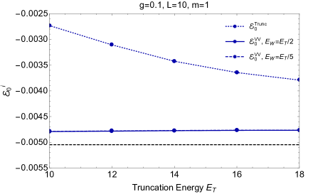
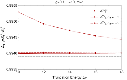
Figure 5: Left: The vacuum energy ${\cal E}_{0}^{i}$ as a function of the truncation energy $E_{T}$ for a coupling of $g=0.1$. Right: Energy difference between the first $\mathds{Z}_{2}$-odd excited state and the vacuum energy ${\cal E}_{0}^{i}$ as a function of the truncation energy for $g=0.1$. In both plots, the dotted curves are computed with the truncated Hamiltonian while the solid and dashed curves are computed with the renormalized hamiltonian at order $VV$. Dashed and dotted lines correspond to the cutoffs $E_{W}=E_{T}/2$ and $E_{W}=E_{T}/5$. We have overlaid two dashed black lines corresponding to the calculation in perturbation theory, see. Eqs. (83) and (84).

First we study the lowest eigenvalues of $H$ at weak coupling, where we can compare with standard perturbation theory. The perturbative corrections to the vacuum and the mass are given by [1]:

$$\Lambda/m^{2} = -\frac{21\xi(3)}{16\pi^{3}}\,\bar{g}^{2}+0.04164(85)\,\bar{g}^{3}+\dots\,,$$ (83)

$$m_{ph}^{2} = m^{2}\big{[}1-\frac{3}{2}\,\bar{g}^{2}+2.86460(20)\,\bar{g}^{3}+\cdots\big{]}\,,$$ (84)

where $\bar{g}\equiv g/m$ and $m_{ph}$ is the physical mass. In Fig. 5 we show the result for the vacuum energy and $m_{ph}$.

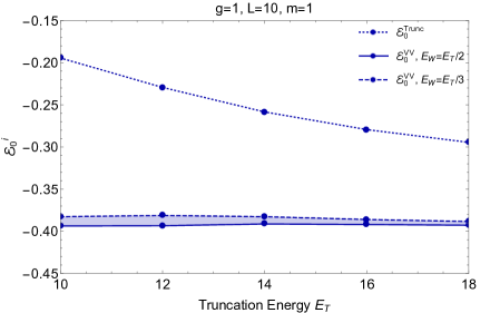
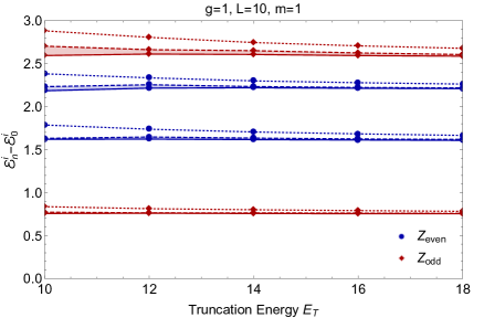
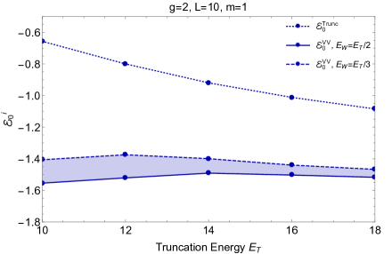
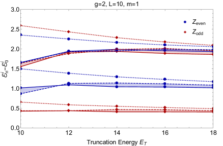
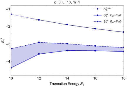
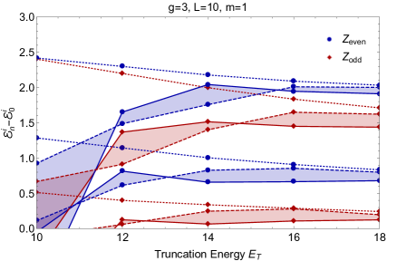
Figure 6: Left: The vacuum energy ${\cal E}_{0}^{i}$ as a function of $E_{T}$ for $g=1$, $2$ and $3$ in descending order. Right: Energy difference between the first excited states and the vacuum energy as a function of the coupling $E_{T}$ for $g=1$, $2$ and $3$. In all the plots of the figure the blue curves correspond to the $\mathds{Z}_{2}$-even sector while the red ones to the $\mathds{Z}_{2}$-odd. The dotted curves are computed with the truncated Hamiltonian, while the solid and dashed lines are computed adding $\Delta H_{2}$ with cutoffs $E_{W}=E_{T}/2$ and $E_{W}=E_{T}/3$.

As explained before, only those entries with $E_{r,s}$ energies below a cutoff $E_{W}$ are renormalized. We do the plot for different values of $E_{W}=E_{T}/2,E_{T}/5$ and we find that the vacuum energy and the physical mass do not depend much on this cutoff. For the left plot the difference between $E_{W}=E_{T}/2$ and $E_{W}=E_{T}/5$ is inappreciable.  We find that the spectrum is much flatter as a function of $E_{T}$ for renormalized eigenvalues than the ones computed with $H_{T}$. Since the exact spectrum is independent of the truncation energy $E_{T}$, a flatter curve in $E_{T}$ indicates a closer value to exact energy levels. However, it could still happen that adding $\Delta H_{3}$ corrections shifted the spectrum by a small amount, as it happens for the $\phi^{2}$ perturbation seen in Figs. 3 and 4 for the range $16\lesssim E_{T}\leq 20$. In the plots we have superimposed constant dashed black lines that are obtained from the perturbative calculations in Eq. (83) and Eq. (84). We find that the eigenvalues computed with $\Delta H_{2}$ are much closer to the perturbative calculation than the ones done with $H_{T}$. The difference between the perturbative result and the one from ${\cal E}^{VV}$ is of ${\cal O}(10^{-4})$ and can be attributed to higher order corrections in the perturbative expansion. Another source of uncertainty comes from higher order $\Delta H_{n}$ corrections not included.

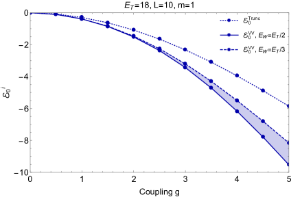
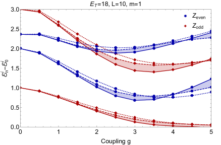
Figure 7: Left: The vacuum energy ${\cal E}_{0}$ as a function of the coupling $g$. Right: Energy difference between the first excited states and the vacuum energy as a function of the coupling constant $g$. In all the plots of the figure the blue curves correspond to the $\mathds{Z}_{2}$-even sector while the red ones to the $\mathds{Z}_{2}$-odd. The dotted curves are computed with the truncated Hamiltonian for a truncation energy $E_{T}=18$, while the solid and dashed lines are computed adding $\Delta H_{2}$ with cutoffs $E_{W}=E_{T}/2$ and $E_{W}=E_{T}/3$.

In Fig. 6 we show plots with different energy levels as a function of the truncation energy $E_{T}$ for $g=1$, $2$, $3$. To compare with previous work, these plots have been done with the same choice of parameters and normalizations as in Figs. (9)-(10) of Ref. [1]. In all the plots the dotted lines are computed using the truncated Hamiltonian while the solid and dashed lines are computed using $\Delta H_{2}$ with $E_{W}=E_{T}/2$ and $E_{W}=E_{T}/3$, respectively. The diamonds and the circles correspond to states in the $\mathds{Z}_{2}$-even and $\mathds{Z}_{2}$-odd sectors of the theory. We find that in all the plots, for high enough values of $E_{T}$, the solid lines for the $\Delta H_{2}$ are flatter than the truncated ones. The difference between the dotted and dashed lines is bigger for the plot for $g=3$ than the one for $g=1$. This can be understood because one expects more overlap from higher $H_{0}$ excited states with the vacuum for higher coupling. The difference between the solid and dashed lines becomes smaller as $E_{T}$ is increased. This can be understood because as $E_{T}$ is increased bigger parts of $(H_{T})_{rs}$ are being renormalized, and eventually the difference between using $E_{W}=E_{T}/2$ and $E_{T}/3$ becomes negligible. An intrinsic error of our calculation of the eigenvalues is the difference between the values obtained for different choices of $E_{W}$. This error could be reduced with a more careful estimate of the expansion parameter $\alpha_{r,s}$, which would be very interesting for the future development of the method. In fact, it seems that for $E_{T}\lesssim 12(14)$ for $g=2(3)$ the cutoff $E_{W}$ is too high (and might include non-perturbative corrections like the one in Eq. (82)) as the eigenvalues deviate a lot from the computation done with $H_{T}$. Another small source of uncertainty in our calculation comes from not having included higher order $\Delta H_{n}$ corrections; in the next section we explain the calculation of $\Delta H_{3}$.

In Fig. 7 we show two plots of the vacuum and first excited states as a function of the coupling constant $g$ for $E_{T}=18$ (cf. Fig. 4 of Ref. [1]). There is an intrinsic uncertainty in our procedure in the choice of $E_{W}$, and as we discussed above it could be lowered by increasing the size of the truncation $E_{T}$ or ideally by refining the determination of $E_{W}$. Notice that the renormalization of the truncated Hamiltonian matters as the solid lines have a significant difference with respect to the truncated (as seen in Fig. 6 the solid lines show a better convergence as a function of $E_{T}$). For $g\gtrsim 3.5$ the first $\mathds{Z}_{2}$-odd excited state seems to become degenerate with the vacuum which is a signal of the spontaneous breaking of the $\mathds{Z}_{2}$ symmetry. This plot can be used to determine the critical coupling, see Ref. [1].

5.4 Three point correction and further comments

As explained in the previous section we have performed the numerical study of the $\phi^{4}$ theory without taking into account the three point correction $\Delta H_{3}$. This would be an interesting point for the future and therefore we give a small preview of the type of expressions one obtains when computing the three point correction. As done throughout the paper, to get the expression for $\Delta H_{3}$ we start by first computing

$$\Delta\widehat{H}_{3}({\cal E})_{rs}=-\lim_{\epsilon\rightarrow 0}\int_{0}^{\infty}dt_{1}dt_{2}\,e^{i({\cal E}-E_{r}+i\epsilon)(t_{1}+t_{2})}{\cal T}\left\{V(T_{1})V(T_{2})V(T_{3})\right\}_{rs}\,,$$ (85)

where $T_{k}=\sum_{n=1}^{3-k}t_{n}$. Then we find $\Delta H_{3}$ by keeping only those terms that have all poles at ${\cal E}>E_{T}$. Then, we see that the three point correction can be split into

$$\Delta H_{3}=\Delta H_{3}^{\mathds{1}}+\Delta H_{3}^{\phi^{2}}+\Delta H_{3}^{\phi^{4}}+\Delta H_{3}^{\phi^{6}}+\Delta H_{3}^{\phi^{8}}+\Delta H_{3}^{\phi^{10}}+\Delta H_{3}^{\phi^{12}}\,,$$ (86)

where the subindices denote the number of fields in each term. The correction $\Delta H_{3}^{\mathds{1}}$ is given by

$$\Delta H_{3}^{\mathds{1}}({\cal E})=\frac{s_{222}\,g^{3}}{(2L)^{6}}\sum_{k_{i},p_{i},l_{i}}\frac{L^{2}\delta_{p_{1}+p_{2}+k_{1}+k_{2},0}^{l_{1}+l_{2}+k_{1}+k_{2},0}}{\omega_{k_{1}}\omega_{k_{2}}\omega_{p_{1}}\omega_{p_{2}}\omega_{l_{1}}\omega_{l_{2}}}\frac{\theta(\Sigma_{i=1}^{2}[\omega_{p_{i}}+\omega_{k_{i}}]-E_{T})}{{\cal E}-\Sigma_{i=1}^{2}[\omega_{p_{i}}+\omega_{k_{i}}]}\frac{\theta(\Sigma_{i=1}^{2}[\omega_{l_{i}}+\omega_{k_{i}}]-E_{T})}{{\cal E}-\Sigma_{i=1}^{2}[\omega_{l_{i}}+\omega_{k_{i}}]}\,.$$ (87)

where the symmetry factor is defined in Eq. (39). The rest of the terms $\Delta H_{3}^{\phi^{2}},\,\cdots,\,\Delta H_{3}^{\phi^{12}}$ can be computed in a similar fashion as explained in previous sections, but we do not present them here since we did not include them in the numerical analysis.

Another interesting thing to study in the future is the local expansion of $\Delta H_{3}$ and higher orders in $\Delta H_{n}$. Here we present some of the terms for the $\Delta H_{3}$ case. As done for $\Delta H_{2}$, when the local expansion applies the calculation is simplified. We use the diagrammatic representation explained in Appendix A for the expressions at ${\cal O}(t^{0},z^{0})$ of the local renormalization. As an example the leading local coefficients that renormalize the operators $V_{2}$, $V_{4}$ and $V_{6}$ are

$$\Delta H_{3+}^{\phi^{2}}\simeq\Big{(}\begin{minipage}[h]{56.37271pt} \vspace{0pt} \includegraphics[width=433.62pt]{./figs/mass1.pdf} \end{minipage}+\begin{minipage}[h]{52.03227pt} \vspace{0pt} \includegraphics[width=433.62pt]{./figs/mass5.pdf} \end{minipage}+\begin{minipage}[h]{52.03227pt} \vspace{0pt} \includegraphics[width=433.62pt]{./figs/mass6.pdf} \end{minipage}+\begin{minipage}[h]{52.03227pt} \vspace{0pt} \includegraphics[width=433.62pt]{./figs/mass3.pdf} \end{minipage}+\cdots\Big{)}\,V_{2}$$ (88)

where for example,

$$\begin{minipage}[h]{52.03227pt} \vspace{0pt} \includegraphics[width=433.62pt]{./figs/mass5.pdf} \end{minipage}=\frac{s_{131}\,g^{3}}{(2L)^{5}}\sum_{k,l,p_{i}}\frac{L^{2}\delta_{p_{1}+p_{2}+p_{3}+k,0}^{l+k,0}}{\omega_{k}\omega_{p_{1}}\omega_{p_{2}}\omega_{p_{3}}}\frac{\theta(\omega_{l}+\omega_{k}-E_{L})}{{\cal E}-\omega_{l}-\omega_{k}}\frac{\theta(\omega_{k}+\Sigma_{i=1}^{3}\omega_{p_{i}}-E_{L})}{{\cal E}-\omega_{k}-\Sigma_{i=1}^{3}p_{i}}\,.$$ (89)

For the renormalization of the quartic we get

$$\Delta H_{3+}^{\phi^{4}}\simeq\Big{(}\begin{minipage}[h]{58.53632pt} \vspace{0pt} \includegraphics[width=433.62pt]{./figs/lambda1.pdf} \end{minipage}+\begin{minipage}[h]{56.37271pt} \vspace{0pt} \includegraphics[width=433.62pt]{./figs/lambda2.pdf} \end{minipage}+\begin{minipage}[h]{56.37271pt} \vspace{0pt} \includegraphics[width=433.62pt]{./figs/lambda3.pdf} \end{minipage}+\cdots\Big{)}\,V_{4}$$ (90)

where for example,

$$= \frac{s_{220}\,g^{3}}{(2L)^{4}}\sum_{l_{1}l_{2}p_{1}p_{2}}\frac{L^{2}\delta_{l_{1}+l_{2},0}^{p_{1}+p_{2},0}}{\omega_{l_{1}}\omega_{l_{2}}\omega_{p_{1}}\omega_{p_{2}}}\frac{\theta(\omega_{l_{1}}+\omega_{l_{2}}-E_{L})}{{\cal E}-\omega_{l_{1}}-\omega_{l_{2}}}\frac{\theta(\omega_{p_{1}}+\omega_{p_{2}}-E_{L})}{{\cal E}-\omega_{p_{1}}-\omega_{p_{2}}}\,.$$ (91)

For $V_{6}$

$$\Delta H_{3+}^{\phi^{6}}\simeq(\begin{minipage}[h]{47.69846pt} \vspace{0pt} \includegraphics[width=433.62pt]{./figs/100peus} \end{minipage}+\cdots)\,V_{6}$$ (92)

where

$$\begin{minipage}[h]{47.69846pt} \vspace{0pt} \includegraphics[width=433.62pt]{./figs/100peus} \end{minipage}=\frac{s_{111}\,g^{3}}{(2L)^{3}}\sum_{k}\frac{L^{2}}{m\,\omega_{k}^{2}}\left(\frac{1}{{\cal E}-2\omega_{k}}\right)^{2}\theta(2\omega_{k}-E_{L})\,.$$ (93)

As final remark, notice that the expression in Eq. (91) is the square of the coefficient of $V_{4}$ (in $\Delta H_{2+}^{\phi^{4}}$) up to a numerical factor (see Eq. (59))

$$\Big{(}\begin{minipage}[h]{36.8606pt} \vspace{0pt} \includegraphics[width=433.62pt]{./figs/Phi42Pt1loop.pdf} \end{minipage}\Big{)}^{2}\,=6g\begin{minipage}[h]{60.70653pt} \vspace{0pt} \includegraphics[width=433.62pt]{./figs/lambda1.pdf} \end{minipage}\,.$$ (94)

It would be very interesting to investigate whether certain classes of diagrams in the $\Delta H_{+}=\sum_{n}\Delta H_{n+}$ expansion can be resumed. This would reduce the error in the computed spectrum and its dependence on the arbitrary truncation energy $E_{T}$. For instance, it could be that the resummation comes only from the leading pieces of the different diagrams. 

5.5 Summary of the method and comparison with Ref. [1]

In this section we summarize our approach to the renormalized Hamiltonian truncation method and briefly comment on the main differences with Ref. [1].

The aim of the renormalized Hamiltonian truncation method is to find the lowest eigenvalues ${\cal E}$ of $H$. This is done by diagonalizing $H_{eff}\equiv H_{T}+\Delta H$, where $H_{T}$ is the truncated Hamiltonian and $\Delta H$ encodes the contributions from the $H_{0}$ eigenstates with $E>E_{T}$. Computing $\Delta H$ is difficult but the problem is simplified if one expands $\Delta H$ in powers of $V_{hh}/H_{hh}$. One expects that the first terms of the series $\Delta H=\sum_{n}\Delta H_{n}$ are a good approximation to $\Delta H$ if the expansion parameter is small. These terms can be computed as explained in Sec. 2, by first finding $\Delta\widehat{H}_{n}$ and keeping only the contributions from the states with $E>E_{T}$. Then, we notice that for some entries with $E_{r},\,E_{s}$ close to $E_{T}$, the series $(\Delta H)_{rs}=\sum_{n}(\Delta H_{n})_{rs}$ is not perturbative (for the chosen parameters $g$, $E_{T}$). We deal with this problem by setting to zero all those entries with $E_{r}$ or $E_{s}>E_{W}$ where $E_{W}$ is chosen appropriately, see Sec. 5.3.

In order to speed up the numerics and gain analytic insight, we perform several approximations to the exact expression of $\Delta H_{2}$. First we introduce a scale $E_{L}$ so that $\Delta H_{2}=\Delta H_{2-}+\Delta H_{2+}$ where $\Delta H_{2+}$ only receives contributions of the states with $E\geq E_{L}$ while $\Delta H_{2-}$ only receives contributions of states with $E_{T}<E<E_{L}$. The scale $E_{L}$ is chosen such that $\Delta H_{2+}$ can be well approximated by the first terms of a local expansion. In our case, we only keep the leading terms $\Delta H_{2+}=\sum_{n=0}^{n=2}c_{2n}\int dx\,\phi^{2n}(x,t)$ and we find that the coefficients $c_{i}$ can be written in terms of phase space functions. Lastly, the coefficients $c_{i}$ are approximated by taking the continuum limit and then expanding them in powers of $m/E_{L}$. On the other hand $\Delta H_{2-}$ is kept exact because its numerical implementation is less costly and it does not admit an approximation by truncating a local expansion. The whole procedure has been described in Sec. 5 and used to do the plots of Sec. 5.3.

Comparison with Ref. [1]

Refs. [1, 3] introduced a renormalized Hamiltonian truncation method by diagonalizing $H_{eff}=H_{T}+\Delta H$ and expanding $\Delta H$ in a series. As explained, we have used this as our starting point. In Ref. [1] though an approximation to $\Delta H_{2}$ is calculated using a different approach than in this paper. To get $\Delta H_{2}$, Ref. [1] starts by defining the following operator $M(E)$

$$M(E)_{rs}\,dE\equiv\sum_{E_{j}\leq E\leq E_{j}+dE}V_{rj}V_{js}\quad\quad\text{such that }\quad\quad\Delta H_{2}=\int_{E_{T}}^{\infty}\,dE\,\frac{M(E)}{{\cal E}-E}\,,$$ (95)

and then noticing that $M(E)$ is related to the matrix element

$$C(\tau)_{rs}\equiv\mathinner{\langle{r}}|V(\tau/2)\,V(-\tau/2)|\mathinner{{s}\,\rangle}=\int_{0}^{\infty}dE\,e^{-[E-(E_{r}+E_{s})/2]\tau}\,M(E)_{rs}$$ (96)

by a Laplace transform. In Ref. [1], the $E\rightarrow\infty$ behavior of $M(E)$ is found by doing the inverse Laplace transform of the non-analytic parts of $C(\tau)$ in the limit $\tau\rightarrow 0$. This is done in the continuum limit, which is a good approximation. The obtained result for $M(E)$ in this limit is taken to compute $\Delta H_{2}$. Ref. [1] differentiates two renormalization procedures, one where the term ($E_{r}+E_{s})/2$ in Eq. (96) is approximated to zero (called local), and one where it is taken into account (called sub-leading). In the later case $M(E)$ is given by $M(E-E_{rs})$, and therefore for entries with $E_{rs}\sim E_{T}$ taking the limit $E-E_{rs}\gg m$ is not justified when $E\sim E_{T}$. The way in which this problem is dealt with is by neglecting all the contributions of $M(E-E_{rs})$ for $E\leq E_{rs}+5m$; in other words, a $\theta(E-E_{rs}-5m)$ is multiplied to the integrand in Eq. (95). 

With this, we can already find the main differences between the two approaches. In our case we calculate the exact expression of $\Delta H_{2}$ which, if needed, can be approximated. Instead, Ref. [1] finds the contributions of $\Delta H_{2}$ that are leading in the limit where $E\rightarrow\infty$ (which neglects the tree and disconnected contributions). From our approach we can recover the local result of Ref. [1] if we set $E_{L}=E_{W}=E_{T}$, neglect the tree and disconnected contributions, take the continuum limit, perform a local expansion to $\Delta H_{2+}$, and make an expansion in $m/E\ll 1$. The choice $E_{L}=E_{T}$ implies $\Delta H_{2}=\Delta H_{2+}$ and $\Delta H_{2-}=0$, while $E_{W}=E_{T}$ means that no entries $(\Delta H_{2})_{rs}$ are set to zero. In a similar way we can recover the sub-leading result taking into account the $E_{rs}$ terms, while introducing by hand a $\theta(E-E_{rs}-5m)$ in the integrals of the coefficients.

Even though the two approaches are quite different, our method and their sub-leading renormalization can still give similar results due to the following. For large enough $E_{T}$, the low entries of $(\Delta H_{2})_{rs}$ only receive contributions from loop-generated operators , and can be well approximated by a local (up to the $E_{rs}$ dependence) expansion even if $E_{L}=E_{T}$. On the other hand, for high energy entries of $(\Delta H_{2})_{rs}$ the tree and disconnected operators are non-zero, and none of the operators can be approximated by a truncated local expansion if $E_{L}=E_{T}$. However, in many cases these high energy entries become non perturbative and we set them to zero when $E_{r}$ or $E_{s}>E_{W}$. Therefore we find that if $E_{W}$ is used, it can be a good approximation for large enough $E_{T}$ to neglect the tree and disconnected terms all together and set $E_{L}=E_{T}$ while performing a local expansion. With this we connect with Ref. [1] where the scale $E_{W}$ is not used to get rid of the non-perturbative contributions. Instead the tree and disconnected terms are neglected, all the entries of $(\Delta H_{2})_{rs}$ are approximated by the loop-generated local (up to $E_{rs}$) operators only and the $\theta(E-E_{rs}-5m)$ is introduced in Eq. (95). As explained, neglecting the tree and disconnected terms is justified, while the introduction of $\theta(E-E_{rs}-5m)$ and truncating the local expansion in practice largely reduce the values of the high energy entries with respect to the exact result. All of these effectively act as our scale $E_{W}$. Therefore we see that in many cases our approach and the one in Ref. [1] can give similar results.

Even though the numerical results are similar, our approach introduces new tools and insights that we think improve the renormalized Hamiltonian truncation method and can help to develop it further.

6 Conclusion and outlook

In this paper we have developed further the Hamiltonian truncation method. In particular we have explained a way to compute the corrections to the truncated Hamiltonian at any order in the large $E_{T}$ expansion of $\Delta H=\sum_{n}\Delta H_{n}$. We have applied these ideas to scalar field theory in two dimensions and studied the spectrum of the theory as a function of the truncation energy and the coupling constant.

There are various open directions that are very interesting and deserve further investigation. Firstly, it would be a great improvement to the method to find a more precise estimate of the expansion parameter of the series. This estimate should be easy to implement numerically and lead to a precise definition of the cutoff $E_{W}$. In this work we have been pragmatic in this respect, and investigated the behaviour of the spectrum as this cutoff is modified. It might be that only removing the contribution of certain type of matrix elements (like the ones corresponding to high occupation number and zero momentum) the series is greatly improved.

We have not pushed the numerical aspects of the method very far and all the computations have been done with Mathematica. With more efficient programming languages it would be interesting to further study and check that as the truncation energy $E_{T}$ is increased the uncertainty in the precise choice of $E_{W}$ is reduced.

Another point that should be addressed is the dependence of the spectrum on $L$ as higher $\Delta H_{n}$ corrections are added; also it could be relevant to inspect if there are diagrams that dominate for large $Lm\gg 1$.

Another very interesting path to develop further is to apply renormalization group techniques to resum the fixed order calculations of $\Delta H$. Since the exact eigenvalues do not depend on the truncation energy $E_{T}$, it may be possible resum the calculation of $\Delta H_{n}$. Our analytic expressions for the $\Delta H_{n}$ corrections permit a precise study of the possible resummation of the leading corrections at each order in the perturbation theory of the large $E_{T}$ expansion. One could start by studying the resummation of the leading local corrections, and for that the phase space formulation that we have introduced is useful as there are simple recursion relations for the differential phase space.

Another fascinating avenue to pursue is the applicability of the method to other theories with higher spin fields and to increase the number of dimensions. In this regard, we notice that the derivation of Eqs. (66)-(68) seems to be formally valid in any space-time dimension $d$. Recall that the $c_{i}$’s are the coefficients of the local operators added to $H_{T}$ to take into account the effect of the highest energetic $H_{0}$ eigenstates not included in the light Hilbert space ${\cal H}_{l}$. As $d$ is increased beyond $d=2$ the UV divergencies appear due to the increasingly rapid growth of the phase space functions $\Phi_{i}(E)$. One can then regulate the $c_{i}$ coefficients with a cutoff $\Lambda$. For instance, consider the coefficient $c_{4}$ of the $\phi^{4}$ operator

$$c_{4}^{\Lambda}({\cal E})=s_{2}\,g_{0}^{2}\ \int_{E_{L}}^{\Lambda}\frac{dE}{2\pi}\,\frac{1}{{\cal E}-E}\,\Phi_{2}(E)\,,$$ (97)

in $d=4$. Then, requiring that the energy levels are independent of the regulator one finds the following $\beta$-function

$$\beta(g)=-\Lambda\frac{\partial c_{4}^{\Lambda}}{\partial\Lambda}+{\cal O}(g^{3})=\frac{s_{2}g^{2}}{2\pi}\Phi_{2}(\Lambda)+{\cal O}(g^{3},{\cal E})\,,$$ (98)

where the ${\cal E}$ corrections can be neglected in the limit of large $\Lambda\gg{\cal E}$. Redefining $g\equiv\lambda/4!$ one recovers the known result for the $\lambda\phi^{4}$ theory $\beta(\lambda)=\frac{3}{16\pi^{2}}\lambda^{2}+{\cal O}(\lambda^{3})\,,$ where we have neglected the mass corrections that for $\Lambda\gg m$ decouple as $\Phi_{2}(\Lambda)=1/(8\pi)+{\cal O}(m^{2}/\Lambda^{2})$. A possible way to make contact between the calculation in the renormalized Hamiltonian method and the standard calculation of the beta function is by noticing that the coefficient of the divergent part of the amplitude is proportional to the coefficient of its finite imaginary part which in turn (by the optical theorem) is proportional to the two-particle phase space. It would be very interesting to further study RG flows from the perspective of the renormalized Hamiltonian truncation method approach.

We think that the Hamiltonian truncation method is a very promising approach to study strong dynamics, and that there are still open important questions to be addressed.

Appendix A Diagramatic representation

There is a simple and powerful diagrammatic representation that permits to easily find the expression for $\Delta H_{n}$. This can be used to either compute the full operator $\Delta H_{n}$ or the leading ${\cal O}(t^{0},z^{0})$ coefficients in the local expansion of $\Delta H_{n+}$ defined in Sec. 4. This representation is valid for any $\phi^{\alpha}$ theory, but here we give examples only for the $\phi^{4}$ case for concreteness.

Local coefficients

Imagine that we want to find the local coefficients ${\cal O}(t^{0},z^{0})$ for $\Delta H_{3+}^{\phi^{2}}$. To find them one puts 3 vertices ordered horizontally  and draws all possible diagrams that have only 2 external lines, four lines meeting at each vertex and don’t have any lines starting and ending at the same vertex. Next, we assign a momentum for each internal line and draw a vertical line between every pair of vertices. One such diagrams is

$$\begin{minipage}[h]{78.04842pt} \vspace{0pt} \includegraphics[width=433.62pt]{./figs/mass1Ex.pdf} \end{minipage}\,.$$ (A.1)

The expression corresponding to a given diagram with $n$ vertices and $N$ propagators is given by

$$sg^{n}\sum_{k^{\prime}s}\frac{1}{\prod_{i=1}^{N}(2L\omega_{k_{i}})}\prod_{p=1}^{n-1}L\,\delta_{p}\frac{\theta\big{(}\sum_{k_{j}\in\{s_{p}\}}\omega_{k_{j}}-E_{L}\big{)}}{{\cal E}-\sum_{k_{j}\in\{s_{p}\}}\omega_{k_{j}}}\,,$$ (A.2)

where $k_{j}=2\pi n_{j}/L$ with $n_{j}\in\mathbb{Z}$. Each of the $n-1$ sets of momenta $\{{s_{p}}\}$ consist in the momenta of the internal lines that are cut by each vertical line. In (A.1) these would be $s_{1}=\{k_{1},k_{2},k_{5}\}$ and $s_{2}=\{k_{3},k_{4},k_{5}\}$. The symbol $\delta_{p}$ stands for a Kronecker delta that imposes that the total momentum crossing a cut is zero; $s$ is a symmetry factor that counts all the ways that the lines of the vertices can be connected to form the diagram. Applying this recipe to the diagram in (A.1) one has

$$\begin{minipage}[h]{69.38078pt} \vspace{0pt} \includegraphics[width=433.62pt]{./figs/mass1Ex.pdf} \end{minipage}=s^{221}_{4}\,g^{3}\sum_{k^{\prime}s}\frac{L^{2}\delta_{k_{1}+k_{2}+k_{5},0}^{k_{3}+k_{4}+k_{5},0}}{\prod_{i=1}^{5}(2L\omega_{k_{i}})}\frac{\theta(\omega_{k_{1}}+\omega_{k_{2}}+\omega_{k_{5}}-E_{L})}{{\cal E}-\omega_{k_{1}}-\omega_{k_{2}}-\omega_{k_{5}}}\frac{\theta(\omega_{k_{3}}+\omega_{k_{4}}+\omega_{k_{5}}-E_{L})}{{\cal E}-\omega_{k_{3}}-\omega_{k_{4}}-\omega_{k_{5}}}\,.\vspace{0.13cm}$$ (A.3)

where the symmetry factor $s_{p}^{mnv}$ is given in Eq. (39). Another example of a contribution to $\Delta H_{3+}^{\phi^{2}}$ would be

$$\begin{minipage}[h]{72.41776pt} \vspace{0pt} \includegraphics[width=433.62pt]{./figs/mass2.pdf} \end{minipage}=s^{212}_{4}\,g^{3}\sum_{k^{\prime}s}\frac{L^{2}\delta_{k_{3}+k_{4}+k_{5},0}^{k_{1}+k_{2}+k_{3}+k_{4},0}}{\prod_{i=1}^{5}(2L\omega_{k_{i}})}\frac{\theta(\Sigma_{s=1}^{5}\omega_{k_{s}}-E_{L})}{{\cal E}-\omega_{k_{1}}-\omega_{k_{2}}-\omega_{k_{3}}-\omega_{k_{4}}}\frac{\theta(\Sigma_{s=1}^{4}\omega_{k_{s}}-E_{L})}{{\cal E}-\omega_{k_{3}}-\omega_{k_{4}}-\omega_{k_{5}}}\,.$$ (A.4)

Notice that the ordering of the vertices matters since the diagrams of (A.3) and (A.4) have the same topology but give different results.

With this prescription one easily recovers Eqs. (55), (57), and (59) corresponding to the $\Delta H_{2+}$ coefficients in the $\phi^{4}$ theory

$$c_{0}=\begin{minipage}[h]{40.75774pt} \vspace{0pt} \includegraphics[width=433.62pt]{./figs/Phi42Pt3loop.pdf} \end{minipage}\,,\quad\quad\quad c_{2}=\begin{minipage}[h]{57.66954pt} \vspace{0pt} \includegraphics[width=433.62pt]{./figs/Phi42Pt2loop.pdf} \end{minipage}\,,\quad\quad\quad c_{4}=\begin{minipage}[h]{52.03227pt} \vspace{0pt} \includegraphics[width=433.62pt]{./figs/Phi42Pt1loop.pdf} \end{minipage}\,.\quad$$ (A.5)

Notice that to include the contributions $E_{rs}$ mentioned at the end of Sec. 5.2 the same diagrammatic representation applies but one must then substitute ${\cal E}\rightarrow{\cal E}-E_{rs}$ in Eq. (A.2) making the coefficients depend on the matrix entry.

Exact $\Delta H_{n}$ opertors

A similar diagrammatic representation can be used to calculate the exact $\Delta\widehat{H}_{n}$ operator from which one can easily get $\Delta H_{n}$. The prescription to follow is very similar to the one for the local case, where one starts drawing the same diagrams and putting vertical lines between every pair of vertices. The only difference is that now one extends the external lines to left and right in all possible combinations for each diagram drawn and also assigns a momentum to the external lines. For the diagram in (A.1) this means

$$\begin{minipage}[h]{69.38078pt} \vspace{0pt} \includegraphics[width=433.62pt]{./figs/home_gordoNL2.pdf} \end{minipage}\quad\quad\begin{minipage}[h]{69.38078pt} \vspace{0pt} \includegraphics[width=433.62pt]{./figs/home_gordoNL1.pdf} \end{minipage}\,\quad\quad\begin{minipage}[h]{69.38078pt} \vspace{0pt} \includegraphics[width=433.62pt]{./figs/home_gordoNL3.pdf} \end{minipage}\,\quad\quad\begin{minipage}[h]{69.38078pt} \vspace{0pt} \includegraphics[width=433.62pt]{./figs/home_gordoNL4.pdf} \end{minipage}\,.$$ (A.6)

Now, the operator corresponding to a given diagram with $n$ vertices, $N$ propagators, $A$ external lines starting left and $B$ external lines starting right is

$$\kappa sg^{n}\sum_{k^{\prime}s,q^{\prime}s}\frac{1}{\prod_{i=1}^{N}(2L\omega_{k_{i}})}\prod_{p=1}^{n-1}\frac{\theta\big{(}\omega_{rs}+\sum_{Q_{j}\in\{s_{p}\}}\omega_{Q_{j}}-E_{L}\big{)}}{{\cal E}-\omega_{rs}-\sum_{Q_{j}\in\{s_{p}\}}\omega_{Q_{j}}}\,\prod_{\alpha=1}^{n}L\delta_{\alpha}\prod_{r=A+1}^{A+B}\frac{a^{\dagger}_{q_{r}}}{\sqrt{2L\omega_{q_{r}}}}\prod_{l=1}^{A}\frac{a_{q_{l}}}{\sqrt{2L\omega_{q_{l}}}}\,,$$ (A.7)

where the sums over $k^{\prime}s,\,q^{\prime}s$ sum over all possible momenta for a given $k_{i},\,q_{i}$. Then, each of the $n-1$ sets of momenta $\{{s_{p}}\}$ consists in the momenta of the lines that are cut by each vertical line. For the first diagram from the left in (A.7) these would be $s_{1}=\{k_{1},k_{2},k_{5}\}$ and $s_{2}=\{k_{3},k_{4},k_{5}\}$, and for the second one $s_{1}=\{q_{1},k_{1},k_{2},k_{5}\}$ and $s_{2}=\{q_{1},k_{3},k_{4},k_{5}\}$. The symbol $\delta_{\alpha}$ stands for a Kronecker delta that imposes momentum conservation at each vertex $\alpha$. The symbol $\omega_{rs}$ depends on the energy of the states $\mathinner{\langle{E_{r}}}|$, $|\mathinner{{E_{s}}\,\rangle}$ on which $a$ and $a^{\dagger}$ act i.e. it is different for each entry $\big{(}a^{\dagger}_{-q_{r}}a_{q_{l}}\big{)}_{rs}$, and is given by $w_{rs}\equiv E_{rs}-\frac{1}{2}\sum_{i=1}^{A+B}\omega_{q_{i}}$ where $E_{rs}=(E_{r}+E_{s})/2$. As before $s$ is a symmetry factor that counts all the ways that the lines of the vertices can be connected to form the diagram. Lastly $\kappa$ counts all the equivalent ways that the external lines coming out from the same vertex can be ordered left and right, for the diagrams in (A.7) is is always one, since there is only one external line per vertex. Applying this recipe to the first and second diagrams in (A.7) one has

$$= s^{221}_{4}\,g^{3}\sum_{k_{1},\cdots,k_{5}}\sum_{q_{1},q_{2}}\frac{L^{2}\delta_{k_{1}+k_{2}+k_{5},q_{1}}^{k_{3}+k_{4}+k_{5},q_{2}}}{\prod_{i=1}^{5}(2L\omega_{k_{i}})}\frac{\theta(\omega_{rs}+\omega_{k_{1}}+\omega_{k_{2}}+\omega_{k_{5}}-E_{L})}{{\cal E}-\omega_{rs}-\omega_{k_{1}}-\omega_{k_{2}}-\omega_{k_{5}}}$$ (A.8)

$$\ \frac{\theta(\omega_{rs}+\omega_{k_{3}}+\omega_{k_{4}}+\omega_{k_{5}}-E_{L})}{{\cal E}-\omega_{rs}-\omega_{k_{3}}-\omega_{k_{4}}-\omega_{k_{5}}}\,L\delta_{k_{3}+k_{4},k_{1}+k_{2}}\frac{a^{\dagger}_{q_{1}}a_{q_{2}}}{2L\sqrt{\omega_{q_{1}}\omega_{q_{2}}}}\,,$$

$$= s^{221}_{4}\,g^{3}\sum_{k_{1},\cdots,k_{5}}\sum_{q_{1},q_{2}}\frac{L^{2}\delta_{k_{1}+k_{2}+k_{5}+q_{1},0}^{k_{3}+k_{4}+k_{5}+q_{1},0}}{\prod_{i=1}^{5}(2L\omega_{k_{i}})}\frac{\theta(\omega_{rs}+\omega_{k_{1}}+\omega_{k_{2}}+\omega_{k_{5}}+\omega_{q_{1}}-E_{L})}{{\cal E}-\omega_{rs}-\omega_{k_{1}}-\omega_{k_{2}}-\omega_{k_{5}}-\omega_{q_{1}}}$$ (A.9)

$$\ \frac{\theta(\omega_{rs}+\omega_{k_{3}}+\omega_{k_{4}}+\omega_{k_{5}}+\omega_{q_{1}}-E_{L})}{{\cal E}-\omega_{rs}-\omega_{k_{3}}-\omega_{k_{4}}-\omega_{k_{5}}-\omega_{q_{1}}}\,L\delta_{q_{1}+q_{2},0}\frac{a^{\dagger}_{-q_{1}}a_{q_{2}}}{2L\sqrt{\omega_{q_{1}}\omega_{q_{2}}}}\,,$$

where $\omega_{rs}=E_{rs}-(\omega_{q_{1}}+\omega_{q_{2}})/2$ and the symmetry factor $s_{p}^{mnv}$ is given in Eq. (39).

With this set of rules one can easily get the expression for $\Delta\widehat{H}_{2}$ and $\Delta\widehat{H}_{3}$ for the $\phi^{2}$ and $\phi^{4}$ theories. Then one finds $\Delta H_{2}$ and $\Delta H_{3}$ by keeping only the contributions with all poles ${\cal E}>E_{T}$.

Appendix B $\Delta H$ for the $\phi^{2}$ perturbation

B.1 Two-point correction

In this section we give the full expressions of the $\Delta\widehat{H}_{2}$ corrections for the scalar theory with potential $V=g_{2}\int dx\phi^{2}$. Recall that the symmetry factor is given by $s_{p}=\binom{2}{p}^{2}p!$. We will use the prescription $E_{rs}=(E_{r}+E_{s})/2$ where $E_{r}$ and $E_{s}$ are $H_{0}$ eigenvalues.

$$\Delta\widehat{H}_{2}^{\mathds{1}}({\cal E})_{rs} = g_{2}^{2}s_{2}\frac{1}{2^{2}}\sum_{k}\frac{1}{\omega_{k}^{2}}\frac{1}{{\cal E}-E_{rs}-2\omega_{k}}\delta_{rs}$$ (B.1)

$$\Delta\widehat{H}_{2}^{\phi^{2}}({\cal E})_{rs} = g_{2}^{2}s_{1}\frac{1}{2^{2}}\sum_{q}\frac{1}{\omega_{q}^{2}}\bigg{[}\left(a_{q}a_{-q}\frac{1}{{\cal E}-E_{rs}-\omega_{q}}+\text{h.c.}\right)\,$$ (B.2)

$$+ \,a^{\dagger}_{q}a_{q}\left(\frac{1}{{\cal E}-E_{rs}-2\omega_{q}}+\frac{1}{{\cal E}-E_{rs}}\right)\bigg{]}$$

$$\Delta\widehat{H}_{2}^{\phi^{4}}({\cal E})_{rs} = g_{2}^{2}s_{0}\frac{1}{2^{2}}\sum_{q_{1},q_{2}}\frac{1}{\omega_{q_{1}}\omega_{q_{2}}}\bigg{[}\,\,a_{q_{1}}a_{q_{2}}a_{-q_{1}}a_{-q_{2}}\frac{1}{{\cal E}-E_{rs}-\omega_{q_{1}}+\omega_{q_{2}}}+\text{h.c.}$$ (B.3)

$$\phantom{g^{2}s_{0}\frac{1}{2^{2}}\sum_{q_{1},q_{2}}}+2\,a^{\dagger}_{q_{1}}a_{q_{1}}a_{q_{2}}a_{-q_{2}}\left(\frac{1}{{\cal E}-E_{rs}+\omega_{q_{2}}}+\frac{1}{{\cal E}-E_{rs}-\omega_{q_{2}}}\right)+\text{h.c.}$$

$$\phantom{g^{2}s_{0}\frac{1}{2^{2}}\sum_{q_{1},q_{2}}}+a^{\dagger}_{q_{1}}a^{\dagger}_{-q_{1}}a_{q_{2}}a_{-q_{2}}\left(\frac{1}{{\cal E}-E_{rs}+\omega_{q_{1}}+\omega_{q_{2}}}+\frac{1}{{\cal E}-E_{rs}-\omega_{q_{1}}-\omega_{q_{2}}}\right)$$

$$\phantom{g^{2}s_{0}\frac{1}{2^{2}}\sum_{q_{1},q_{2}}}+4\,a^{\dagger}_{q_{1}}a^{\dagger}_{q_{2}}a_{q_{1}}a_{q_{2}}\frac{1}{{\cal E}-E_{rs}}\,\bigg{]}\,.$$

B.2 Three-point correction

In this section we give the full expressions of the $\Delta H_{3}$ corrections for the scalar theory with potential $V=g_{2}\int dx\phi^{2}$. Recall that the symmetry factor is given by

$$s^{mnv}_{p}=\frac{p!^{3}}{(p-m-n)!(p-m-v)!(p-n-v)!m!n!v!}\,.$$ (B.4)

We use the notation $\Delta H_{3}=\Delta H_{3}^{\mathds{1}}+\Delta H_{3}^{\phi^{2}}+\Delta H_{3}^{\phi^{4}}+\Delta H_{3}^{\phi^{6}}$, where

$$\Delta H_{3}^{\mathds{1}}({\cal E})_{rs} = \frac{g_{2}^{3}s_{2}^{111}}{2^{3}}\sum_{k}\frac{1}{\omega_{k_{1}}\omega_{k_{2}}\omega_{k_{3}}}G_{0}(k_{1},k_{2},k_{3},E_{T})\,,$$ (B.5)

$$\Delta H_{3}^{\phi^{2}}({\cal E})_{rs} = \frac{g_{2}^{3}}{2^{3}}\sum_{k,q}\frac{1}{\omega_{k_{1}}\omega_{k_{2}}}\frac{1}{\sqrt{\omega_{q_{1}}\omega_{q_{2}}}}\big{[}s_{2}^{200}G_{2,1}(k_{1},k_{2},q_{1},q_{2},E_{T})$$ (B.6)

$$+s_{2}^{110}G_{2,2}(k_{1},k_{2},q_{1},q_{2},E_{T})\big{]}\,,$$

$$\Delta H_{3}^{\phi^{4}}({\cal E})_{rs} = \frac{g_{2}^{3}s_{2}^{100}}{2^{3}}\sum_{k,q}\frac{1}{\omega_{k}}\frac{1}{\sqrt{\omega_{q_{1}}\cdots\omega_{q_{4}}}}G_{4}(k,q_{1},\dots,q_{4})\,,$$ (B.7)

$$\Delta H_{3}^{\phi^{6}}({\cal E})_{rs} = \frac{g_{2}^{3}s_{2}^{000}}{2^{3}}\sum_{q}\frac{1}{\sqrt{\omega_{q_{1}}\cdots\omega_{q_{6}}}}G_{6}(q_{1},\dots,q_{6})\,,$$ (B.8)

where

$$G_{0} = \delta_{k_{1}+k_{2},0}\delta_{k_{1}+k_{3},0}\,[f_{0}]^{12}[f_{0}]^{13}\,,$$ (B.9)

$$G_{2,1} = a_{q_{1}}a_{q_{2}}\,\delta_{0}\delta_{k_{1}+k_{2},0}\,[f_{2}]^{12}_{12}[f_{2}]^{12}\,+\text{h.c.}+2a^{\dagger}_{q_{1}}a_{q_{2}}\,\delta_{1}\delta_{k_{1}+k_{2},0}\,[f_{2}]^{12}_{1}[f_{2}]^{12}_{2}\,,$$ (B.10)

$$G_{2,2} = a^{\dagger}_{q_{1}}a_{q_{2}}\,\delta_{1}\delta_{k_{1}+q_{1},0}\delta_{k_{1}+k_{2},0}\,\left([f_{2}]^{1}_{12}[f_{2}]^{12}_{1}+[f_{2}]^{1}_{12}[f_{2}]^{12}_{2}+[f_{2}]^{1}_{12}[f_{2}]^{2}_{12}\right)\,,$$ (B.11)

$$G_{4} = a^{\dagger}_{q_{1}}a_{q_{2}}a_{q_{3}}a_{q_{4}}\,\delta_{1}\delta_{k+q_{1},0}\delta_{q_{3}+q_{4},0}[f_{4}]^{1}_{1234}[f_{4}]^{1}_{12}\,+\text{h.c.}\,$$ (B.12)

$$+ 2a^{\dagger}_{q_{1}}a^{\dagger}_{q_{2}}a_{q_{3}}a_{q_{4}}\,\delta_{2}\delta_{q_{1}-q_{3},0}\delta_{k+q_{2},0}[f_{4}]^{1}_{124}[f_{4}]^{1}_{234}$$

$$+ a^{\dagger}_{q_{1}}a^{\dagger}_{q_{2}}a_{q_{3}}a_{q_{4}}\,\delta_{2}\left(\delta_{q_{1}+q_{2},0}\delta_{k+q_{4},0}[f_{4}]_{1234}[f_{4}]^{1}_{124}+\delta_{q_{3}+q_{4},0}\delta_{k+q_{1},0}[f_{4}]_{1234}[f_{4}]^{1}_{124}\right)\,,\quad\quad$$

$$G_{6} = a^{\dagger}_{q_{1}}a^{\dagger}_{q_{2}}a_{q_{3}}a_{q_{4}}a_{q_{5}}a_{q_{6}}\,\delta_{2}\delta_{q_{1}+q_{2},0}\delta_{q_{3}+q_{4},0}[f_{6}]_{123456}[f_{6}]_{1234}\,+\text{h.c.}\,$$ (B.13)

$$+ 2a^{\dagger}_{q_{1}}a^{\dagger}_{q_{2}}a^{\dagger}_{q_{3}}a_{q_{4}}a_{q_{5}}a_{q_{6}}\,\delta_{3}\delta_{q_{1}+q_{2},0}\delta_{q_{5}+q_{6},0}[f_{6}]_{12356}[f_{6}]_{12456}\,\,.$$

We have defined $w_{rs}^{p}\equiv E_{rs}-\frac{1}{2}\sum_{i=1}^{p}\omega_{q_{i}}$, $\delta_{d}\equiv\delta_{\Sigma_{i=1}^{d}q_{i},\Sigma_{j=d+1}^{p}q_{j}}$ (the Kronecker delta that imposes momentum conservation to the creation/annihilation operators) and

$$[f_{p}]_{Q}^{K}=\frac{\theta(\omega_{rs}^{p}+\Sigma_{i\in\{Q\}}\omega_{q_{i}}+\Sigma_{i\in\{K\}}\omega_{k_{i}}-E_{T})}{{\cal E}-\omega_{rs}^{p}-\sum_{i\in\{Q\}}\omega_{q_{i}}-\sum_{i\in\{K\}}\omega_{k_{i}}}\,.$$ (B.14)

Appendix C $\Delta H$ for the $\phi^{4}$ theory

In this appendix we give the exact two-point correction and the first terms in the local expansion of the three-point correction. Getting the exact three-point correction would be straightforward.

C.1 Two-point correction

In this appendix we give the full expressions of the $\Delta H_{2}$ for the $\phi^{4}$ theory. Using the notation $\Delta H_{2}=\sum_{n=0}^{8}\Delta H_{2}^{\phi^{n}}$ we have

$$\Delta H_{2}^{\mathds{1}}({\cal E},E_{T}) = \frac{s_{4}g^{2}}{2^{4}L^{2}}\sum_{k_{1}k_{2}k_{3}k_{4}}\frac{1}{\omega_{k_{1}}\omega_{k_{2}}\omega_{k_{3}}\omega_{k_{4}}}F_{0}(k_{1},k_{2},k_{3},k_{4},E_{T})\,,$$ (C.1)

$$\Delta H_{2}^{\phi^{2}}({\cal E},E_{T}) = \frac{s_{3}g^{2}}{2^{4}L^{2}}\sum_{k_{1},k_{2},k_{3}}\sum_{q_{1},q_{2}}\,\frac{1}{\omega_{k_{1}}\omega_{k_{2}}\omega_{k_{3}}}\frac{1}{\sqrt{\omega_{q_{1}}\omega_{q_{2}}}}F_{2}(k_{1},k_{2},k_{3},q_{1},q_{2},E_{T})\,,$$ (C.2)

$$\Delta H_{2}^{\phi^{4}}({\cal E},E_{T}) = \frac{s_{2}g^{2}}{2^{4}L^{2}}\sum_{k_{1},k_{2}}\sum_{q_{1},q_{2},q_{3},q_{4}}\,\frac{1}{\omega_{k_{1}}\omega_{k_{2}}}\frac{1}{\sqrt{\omega_{q_{1}}\cdots\omega_{q_{4}}}}F_{4}(k_{1},k_{2},q_{1},\dots,q_{4},E_{T})\,,$$ (C.3)

$$\Delta H_{2}^{\phi^{6}}({\cal E},E_{T}) = \frac{s_{1}g^{2}}{2^{4}L^{2}}\sum_{k}\sum_{q_{1},\dots,q_{6}}\,\frac{1}{\omega_{k}}\frac{1}{\sqrt{\omega_{q_{1}}\dots\omega_{q_{6}}}}F_{6}(k,q_{1},q_{2},\dots,q_{6},E_{T})\,,$$ (C.4)

$$\Delta H_{2}^{\phi^{8}}({\cal E},E_{T}) = \frac{s_{0}g^{2}}{2^{4}L^{2}}\sum_{q_{1},\dots,q_{8}}\,\frac{1}{\sqrt{\omega_{q_{1}}\cdots\omega_{q_{8}}}}F_{8}(q_{1},q_{2},\dots,q_{8},E_{T})$$ (C.5)

The $F_{i}$ functions are given by

$$F_{0} = \delta_{k_{1}+k_{2}+k_{3}+k_{4},0}\,[f_{0}]^{1234}$$ (C.6)

$$F_{2} = a^{\dagger}_{q_{1}}a_{q_{2}}\,\delta_{1}\,\delta_{k_{1}+k_{2}+k_{3},q_{1}}\left(\,[f_{2}]^{123}+[f_{2}]^{123}_{12}\,\right)+a_{q_{1}}a_{q_{2}}\,\delta_{0}\,\delta_{k_{1}+k_{2}+k_{3},q_{1}}\,[f_{2}]^{123}_{2}\,+\,\text{h.c.}\,$$ (C.7)

$$F_{4} = a_{q_{1}}a_{q_{2}}a_{q_{3}}a_{q_{4}}\,\delta_{0}\,\delta_{k_{1}+k_{2},q_{1}+q_{2}}[f_{4}]^{12}_{34}+\text{h.c.}$$ (C.8)

$$+ 2a^{\dagger}_{q_{1}}a_{q_{2}}a_{q_{3}}a_{q_{4}}\,\delta_{1}\,\left(\,\delta_{k_{1}+k_{2},q_{1}-q_{2}}[f_{4}]^{12}_{2}+\delta_{k_{1}+k_{2},-q_{1}+q_{2}}[f_{4}]^{12}_{134}\,\right)+\text{h.c.}$$

$$+ a^{\dagger}_{q_{1}}a^{\dagger}_{q_{2}}a_{q_{3}}a_{q_{4}}\,\delta_{2}\,\big{(}\,\delta_{k_{1}+k_{2},q_{1}+q_{2}}\,[f_{4}]^{12}+\delta_{k_{1}+k_{2},-q_{1}-q_{2}}[f_{4}]^{12}_{1234}\,\,+\,4\,\delta_{k_{1}+k_{2},q_{1}-q_{3}}[f_{4}]^{12}_{14}\big{)}$$

$$F_{6} = a^{\dagger}_{q_{1}}a_{q_{2}}a_{q_{3}}a_{q_{4}}a_{q_{5}}a_{q_{6}}\,\delta_{1}\,\delta_{k,q_{2}+q_{3}-q_{1}}\,3\,[f_{6}]^{1}_{1456}\,+\text{h.c.}$$

$$+ a^{\dagger}_{q_{1}}a^{\dagger}_{q_{2}}a_{q_{3}}a_{q_{4}}a_{q_{5}}a_{q_{6}}\,\delta_{2}\left(\,9\,\delta_{k,q_{3}+q_{4}-q_{1}}[f_{6}]^{1}_{156}+3\,\delta_{k,q_{3}-q_{1}-q_{2}}[f_{6}]^{1}_{12456}\,\right)\,+\text{h.c.}$$

$$+ a^{\dagger}_{q_{1}}a^{\dagger}_{q_{2}}a^{\dagger}_{q_{3}}a_{q_{4}}a_{q_{5}}a_{q_{6}}\,\delta_{3}\,\big{(}\,9\,\delta_{k,q_{4}+q_{5}-q_{1}}[f_{6}]^{1}_{16}+9\delta_{k,-q_{4}-q_{5}+q_{1}}[f_{6}]^{1}_{2345}\,+\delta_{k+q_{1}+q_{2}+q_{3},0}[f_{6}]^{1}_{123456}\,\big{)}$$

$$F_{8} = a^{\dagger}_{q_{1}}a^{\dagger}_{q_{2}}a_{q_{3}}a_{q_{4}}a_{q_{5}}a_{q_{6}}a_{q_{7}}a_{q_{8}}\,\delta_{2}\,6\delta_{q_{1}+q_{2}-q_{3}-q_{4},0}[f_{8}]_{125678}\,+\,\text{h.c.}$$ (C.10)

$$+ a^{\dagger}_{q_{1}}a^{\dagger}_{q_{2}}a^{\dagger}_{q_{3}}a_{q_{4}}a_{q_{5}}a_{q_{6}}a_{q_{7}}a_{q_{8}}\,\delta_{3}\big{(}24\delta_{q_{1}+q_{2}-q_{4}-q_{5}}[f_{8}]_{12678}\,+\,4\delta_{q_{1}+q_{2}+q_{3}-q_{4}}[f_{8}]_{1235678}\,\big{)}+\text{h.c.}$$

$$+ a^{\dagger}_{q_{1}}a^{\dagger}_{q_{2}}a^{\dagger}_{q_{3}}a^{\dagger}_{q_{4}}a_{q_{5}}a_{q_{6}}a_{q_{7}}a_{q_{8}}\,\delta_{4}\big{(}\,16\delta_{q_{1}-q_{5}-q_{6}-q_{7},0}\left([f_{8}]_{18}+[f_{8}]_{234567}\right)$$

$$+ 36\delta_{q_{1}+q_{2}-q_{5}-q_{6},0}[f_{8}]_{1278}+\delta_{q_{1}+q_{2}+q_{3}+q_{4},0}[f_{8}]_{12345678}\,\big{)}\,.$$

We have defined $w_{rs}^{p}\equiv E_{rs}-\frac{1}{2}\sum_{i=1}^{p}\omega_{q_{i}}$, $\delta_{d}\equiv\delta_{\Sigma_{i=1}^{d}q_{i},\Sigma_{j=d+1}^{p}q_{j}}$ (the Kronecker delta that imposes momentum conservation to the creation/annihilation operators) and

$$[f_{p}]_{Q}^{K}=\frac{\theta(\omega_{rs}^{p}+\Sigma_{i\in\{Q\}}\omega_{q_{i}}+\Sigma_{i\in\{K\}}\omega_{k_{i}}-E_{T})}{{\cal E}-\omega_{rs}^{p}-\sum_{i\in\{Q\}}\omega_{q_{i}}-\sum_{i\in\{K\}}\omega_{k_{i}}}\,.$$ (C.11)

References

- [1] S. Rychkov and L. G. Vitale, Phys. Rev. D 91 (2015) 8, 085011 [arXiv:1412.3460 [hep-th]].
- [2] S. Rychkov and L. G. Vitale, arXiv:1512.00493 [hep-th].
- [3] M. Hogervorst, S. Rychkov and B. C. van Rees, Phys. Rev. D 91 (2015) 025005 [arXiv:1409.1581 [hep-th]].
- [4] V. P. Yurov and A. B. Zamolodchikov, Int. J. Mod. Phys. A 5 (1990) 3221.
- [5] S. J. Brodsky, H. C. Pauli and S. S. Pinsky, Phys. Rept. 301 (1998) 299 [hep-ph/9705477].
- [6] D. Lee, N. Salwen, and D. Lee, “The Diagonalization of quantum field Hamiltonians,” Phys.Lett. B503 (2001) 223–235, arXiv:hep-th/0002251 [hep-th].
- [7] D. Lee, N. Salwen, and M. Windoloski, “Introduction to stochastic error correction methods,” Phys.Lett. B502 (2001) 329–337, arXiv:hep-lat/0010039 [hep-lat].
- [8] N. Salwen, Non-perturbative methods in modal field theory. arXiv:hep-lat/0212035 [hep-lat]. Ph.D. thesis, Harvard University, 2001.
- [9] M. Windoloski, A Non-perturbative Study of Three-Dimensional Quartic Scalar Field Theory Using Modal Field Theory. Ph.D. thesis, University of Massachusetts Amherst, 2000.
- [10] I. Brooks, E.D. and S. C. Frautschi, “Scalars Coupled to Fermions in (1+1)-dimensions,” Z.Phys. C23 (1984) 263.
- [11] E. Katz, G. M. Tavares, and Y. Xu, “Solving 2D QCD with an adjoint fermion analytically,” JHEP 1405 (2014) 143, arXiv:1308.4980 [hep-th].
- [12] E. Katz, G. M. Tavares, and Y. Xu, “A solution of 2D QCD at Finite using a conformal basis,” arXiv:1405.6727 [hep-th].
- [13] S. Chabysheva and J. Hiller, “Basis of symmetric polynomials for many-boson light-front wave functions,” arXiv:1409.6333 [hep-ph].
- [14] P. Giokas and G. Watts, “The renormalisation group for the truncated conformal space approach on the cylinder,” arXiv:1106.2448 [hep-th].
- [15] M. Lencses and G. Takacs, “Excited state TBA and renormalized TCSA in the scaling Potts model,” JHEP 09 (2014) 052, arXiv:1405.3157 [hep-th].
- [16] A. Coser, M. Beria, G. P. Brandino, R. M. Konik and G. Mussardo, J. Stat. Mech. 1412 (2014) P12010 arXiv:1409.1494 [hep-th].
- [17] M. Lencses and G. Takacs, JHEP 1509 (2015) 146 arXiv:1506.06477 [hep-th].
- [18] M. Luscher, Commun. Math. Phys. 104 (1986) 177.
- [19] M. Luscher, Commun. Math. Phys. 105 (1986) 153.