PoS(LATTICE2015)264
ADP-15-51/T953
DESY 15-224
Edinburgh 2015/32
Liverpool LTH 1071

Determining the scale in Lattice QCD

Abstract:

We discuss scale setting in the context of 2+1 dynamical fermion simulations where we approach the physical point in the quark mass plane keeping the average quark mass constant. We have simulations at four beta values, and after determining the paths and lattice spacings, we give an estimation of the phenomenological values of various Wilson flow scales.

1 Singlet quantities

Numerical lattice QCD simulations determine mass (or other) ratios but not the scale itself, which has to be determined from experiment. A hadron mass such as the proton mass or decay constant such as the pion decay constant are often used for this purpose. We discuss here the advantages of setting the scale using a flavour-singlet quantity, which in conjunction with simulations keeping the average quark mass constant allow $SU(3)$ flavour breaking expansions to be used. This is illustrated using $2+1$ flavour clover fermions, and in addition a determination of the Wilson flow scales, $\sqrt{t_{0}^{\exp}}$ and $w_{0}^{\exp}$ is given.

This talk is based on [1], where further details can be found.

Dynamical simulations start with some values of the quark masses and then extrapolate along some path in $(u,d,s)$ space to the physical point. The strategy we have adopted here, [2, 3] is to start at a point on the $SU(3)$ flavour symmetric line, when all the quark masses are equal

$$(m_{0},m_{0},m_{0})\to(m_{u}^{*},m_{d}^{*},m_{s}^{*})\,,$$ (1)

and to keep the singlet quark mass $\overline{m}$ constant

$$\overline{m}={1\over 3}\,\left(m_{u}+m_{d}+m_{s}\right)=\mbox{const.}\equiv m_{0}\,.$$ (2)

This allows an $SU(3)_{F}$ flavour symmetry breaking expansion for masses and matrix elements. The expansion parameter is naturally the distance from the $SU(3)$ flavour plane, parametrised by

$$\delta m_{q}=m_{q}-\overline{m}\,.$$ (3)

This has the trivial constraint

$$\delta m_{u}+\delta m_{d}+\delta m_{s}=0\,.$$ (4)

The expansion coefficients are functions of $\overline{m}$ only so provided $\overline{m}$ is kept constant they remain unaltered whether we have mass degenerate $u$ and $d$ quarks or not. This opens the possibility of determining isospin breaking quantities from just $2+1$ simulations. The plane (or path) is called ‘unitary’ if we expand in both the same sea and valence quarks masses.

Consider now a flavour singlet quantity $X_{S}(m_{u},m_{d},m_{s})$ which by definition is invariant under $u$, $d$, $s$ permutations. This has a stationary point about the $SU(3)$ flavour symmetric line. For upon expanding a flavour singlet quantity about a point on the $SU(3)$-flavour line we have

$$X_{S}(\overline{m}+\delta m_{u},\overline{m}+\delta m_{d},\overline{m}+\delta m_{s})$$ (5)

$$= X_{S}(\overline{m},\overline{m},\overline{m})+\left.{\partial X_{S}\over\partial m_{u}}\right|_{0}\,\delta m_{u}+\left.{\partial X_{S}\over\partial m_{d}}\right|_{0}\,\delta m_{d}+\left.{\partial X_{S}\over\partial m_{s}}\right|_{0}\,\delta m_{s}+O((\delta m_{q})^{2})\,.$$

However on this line all the above derivatives are equal and thus we have

$$X_{S}(\overline{m}+\delta m_{u},\overline{m}+\delta m_{d},\overline{m}+\delta m_{s})=X_{S}(\overline{m},\overline{m},\overline{m})+O((\delta m_{q})^{2})\,.$$ (6)

There are many possibilities for singlet quantities. Using hadronic masses we have, for example

$$X_{N}^{2} = \mbox{\small$\frac{1}{6}$}(M_{p}^{2}+M_{n}^{2}+M_{\Sigma^{+}}^{2}+M_{\Sigma^{-}}^{2}+M_{\Xi^{0}}^{2}+M_{\Xi^{-}}^{2})=(1.1610\,\mbox{GeV})^{2}$$

$$X_{\pi}^{2} = \mbox{\small$\frac{1}{6}$}(M_{K^{+}}^{2}+M_{K^{0}}^{2}+M_{\pi^{+}}^{2}+M_{\pi^{-}}^{2}+M_{\overline{K}^{0}}^{2}+M_{K^{-}}^{2})=(0.4116\,\mbox{GeV})^{2}$$

$$X_{\rho}^{2} = \mbox{\small$\frac{1}{6}$}(M_{K^{*+}}^{2}+M_{K^{*0}}^{2}+M_{\rho^{+}}^{2}+M_{\rho^{-}}^{2}+M_{\overline{K}^{*0}}^{2}+M_{K^{*-}}^{2})=(0.8562\,\mbox{GeV})^{2}\,,$$ (7)

for octet baryons, pseudoscalar octet mesons and vector octet mesons respectively. Another baryon octet possibilty is $X_{\Lambda}^{2}=\mbox{\small$\frac{1}{2}$}(M_{\Sigma}^{2}+M_{\Lambda}^{2})$ but other singlet quantities can be constructed using the baryon decuplet. Alternatively gluonic quantities can be used such as the ‘Force’ scale $X_{r_{0}}^{2}=1/r_{0}^{2}$ or the Wilson flow scales, introduced by Lüscher

$$X_{t_{0}}^{2}={1\over t_{0}}\,,\qquad X_{w_{0}}^{2}={1\over w_{0}^{2}}\,,$$ (8)

(see e.g. [4, 5]). These are all ‘secondary scales’, their physical value has to be determined.

The stationary point of $X_{S}$ can be checked, using the Gell-Mann–Okubo $SU(3)$ flavour breaking expansion. For example for the pseudoscalar octet mesons we have the expansion

$$M_{\pi^{+}}^{2}(=M_{\pi^{-}}^{2}) = M_{0\pi}^{2}+\alpha_{\pi}(\delta m_{u}+\delta m_{d})+O((\delta m_{q})^{2})$$

$$M_{K^{+}}^{2}(=M_{K^{-}}^{2}) = M_{0\pi}^{2}+\alpha_{\pi}(\delta m_{u}+\delta m_{s})+O((\delta m_{q})^{2})$$

$$M_{K^{0}}^{2}(=M_{\overline{K}^{0}}^{2}) = M_{0\pi}^{2}+\alpha_{\pi}(\delta m_{d}+\delta m_{s})+O((\delta m_{q})^{2})\,.$$ (9)

Constructing $X_{\pi}^{2}$ gives immediately the result of eq. (5). Another check is to use $\chi$-PT (assuming that it is valid in the neighbourhood of the $SU(3)$ flavour plane/line). Simply choose your favourite $\chi$-PT result and expand about a $SU(3)$ flavour symmetric line/point. For example in [6], the chiral expansion for $t_{0}$ (for mass degenerate $u$ and $d$ quarks) can be manipulated [1] to give

$$t_{0}=T(\overline{\chi})\left[1+{1\over(4\pi f_{0})^{4}}(\textstyle{5\over 6}k_{2}+\textstyle{1\over 4}k_{5}^{\prime\prime})(\chi_{s}-\chi_{l})^{2}+\cdots\right]\,,$$ (10)

where $T$ is a (known) function of $\overline{\chi}\equiv 1/3\,(2\chi_{l}+\chi_{s})$ only. As $(\chi_{s}-\chi_{l})\propto(\delta m_{s}-\delta m_{l})$ then this agrees with our previous assertion: there is no linear term, the first term is quadratic in $SU(3)$ flavour symmetry breaking.

2 Lattice matters

We have generated $2+1$ flavour gauge configurations using an action consisting of tree level Symanzik glue and a mildy stout smeared $O(a)$ non-perturbatively improved clover action, [7], at four-$\beta$ values, $\beta=5.40,5.50,5.65,5.80$ on a variety of lattice sizes $24^{3}\times 48$, $32^{3}\times 64$ and $48^{3}\times 96$. All box sizes have $L\mathrel{\hbox to0.0pt{\lower 4.0pt\hbox{\hskip 1.0pt$\sim$}\hss}\raise 1.0pt\hbox{$>$}}2\,\mbox{fm}$. All the pion masses used have $M_{\pi}L>4$ and range from about $500$ to $220\,\mbox{MeV}$. They are either at points on the $SU(3)$ flavour symmetric line or along lines of constant $\overline{m}$. This gives $21$ data sets at our disposal.

The quark mass $m_{q}$ and $\delta m_{q}$ are given by

$$m_{q}={1\over 2}\left({1\over\kappa_{q}}-{1\over\kappa_{0c}}\right)\,,\qquad\delta m_{q}=m_{q}-\overline{m}={1\over 2}\left({1\over\kappa_{q}}-{1\over\kappa_{0}}\right)\,,$$ (11)

where $\kappa_{0c}$ is chiral limit along symmetric line. (Note that this cancels in $\delta m_{q}$.)

We first investigate the constancy of singlet quantities, as given in eq. (6). In Fig. 1

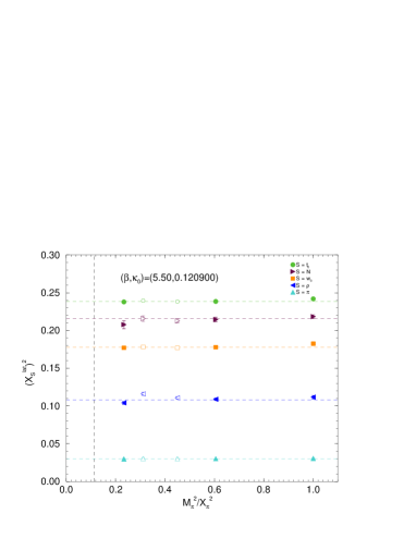
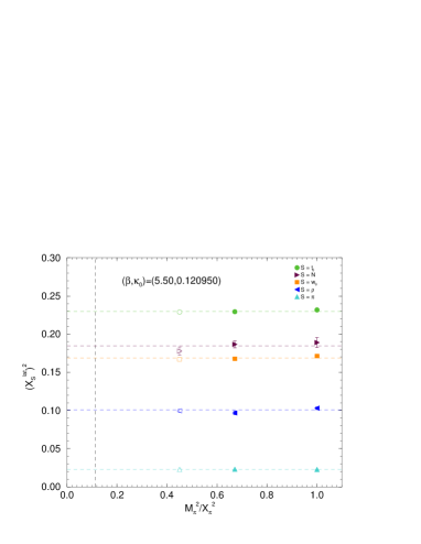
Figure 1: Top to bottom $(X_{S}^{\rm lat})^{2}$ for $S=t_{0}$ (circles), $N$ (right triangles), $w_{0}$ (squares), $\rho$ (left triangles) and $\pi$ (up triangles) for $(\beta,\kappa_{0})=(5.50,0.120900)$ (left panel) and $(\beta,\kappa_{0})=(5.50,0.120950)$ (right panel) together with constant fits. The opaque points have $M_{\pi}L<4$ and are not included in the fits. The vertical line represents the physical point.

we plot $(X_{S}^{\rm lat})^{2}$ for $S=t_{0}$, $N$, $w_{0}$, $\rho$ and $\pi$ for $(\beta,\kappa_{0})=(5.50,0.120900)$, $(5.50,0.120950)$. As expected, in agreement with the discussion of section 1, the $X_{S}^{2}$ singlet quantities are constant.

We now take $X_{S}=\mbox{const.}$ to determine the scale

$$a_{S}^{2}(\kappa_{0})={X_{S}^{\rm lat\,2}(\kappa_{0})\over X_{S}^{\exp\,2}}\,.$$ (12)

This is a function of $m_{0}$ or here $\kappa_{0}$. So if we vary $\kappa_{0}$ (for example as in Fig. 1) – when pairs $a_{S}$, $a_{S^{\prime}}$ cross this gives a common lattice spacing $a$. We apply this in particular here to

$$(S,S^{\prime})=(\pi,N),\,(\pi,\rho)\,.$$ (13)

For $S=t_{0}$, $w_{0}$ we can arrange $X_{t_{0}}^{\exp}$, $X_{w_{0}}^{\exp}$ (from eq. (12)) so that these singlet quantities also cross at the same point. In Fig. 2 we show these crossings

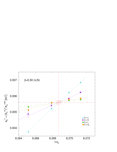
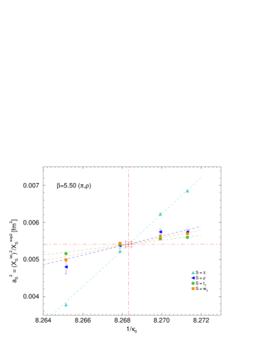
Figure 2: $a_{S}^{2}$ against $1/\kappa_{0}$ for $S=\pi$, $N$ and $t_{0}$, $w_{0}$ together with quadratic fits for $\beta=5.50$. Left panel: based on $(\pi,N)$ crossing; Right panel: based on $(\pi,\rho)$ crossing.

for $\beta=5.50$. From the results for the four beta values we can now make the last, continuum extrapolation. This is shown in Fig. 3.

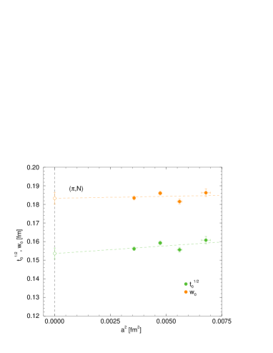
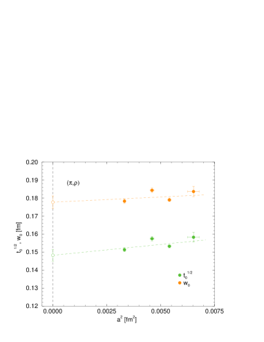
Figure 3: $\sqrt{t_{0}}$ and $w_{0}$ (in fm) against $a^{2}$ (in $\mbox{fm}^{2}$) from the $(\pi,N)$ crossing (left panel) and $(\pi,\rho)$ (right panel) crossing together with a linear fit.

A (weighted) average of these results gives our final estimates for $\sqrt{t_{0}^{\exp}}$, $w_{0}^{\exp}$ as found in [1].

Alternatively we can write

$${2M_{K}^{2}-M_{\pi}^{2}\over X^{2}_{S}}=C-2{M_{\pi}^{2}\over X_{S}^{2}}\,,$$ (14)

($C=X_{\pi}^{2}/X_{S}^{2}$) for $S=N,\rho,t_{0},w_{0}$. In Fig. 4 we

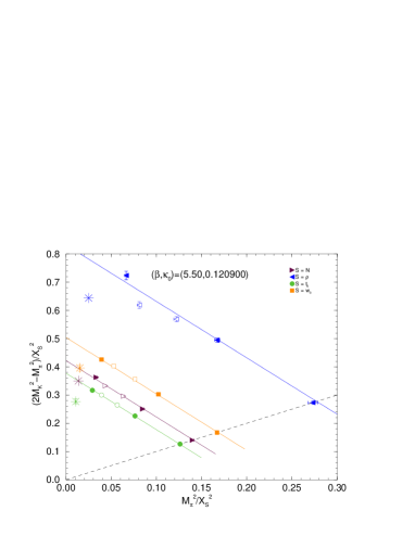
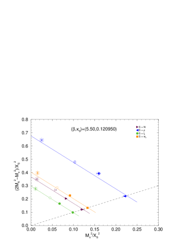
Figure 4: $(2M_{K}^{2}-M_{\pi}^{2})/X^{2}_{S}$ against $M_{\pi}^{2}/X_{S}^{2}$, together with the fit from eq. (14) for $(\beta,\kappa_{0})=(5.50,0.120900)$ (left panel) and $(5.50,0.120950)$ (right panel). The stars correspond to the phenomenological values.

plot this function for $(\beta,\kappa_{0})=(5.50,0.120900)$, $(5.50,0.120950)$. This represents the path in the quark mass plane. Also shown are the experimental values (now including those of $S=t_{0}$, $w_{0}$). We see that these $\kappa_{0}$ values straddle the optimum $\kappa_{0}^{*}$ – it is clear that $\kappa_{0}^{*}$ lies closer to $0.120950$ than $0.120900$.

Finally we comment on our results. In the left panel of Fig. 5 we plot $a^{2}$ against $g_{0}^{2}$.

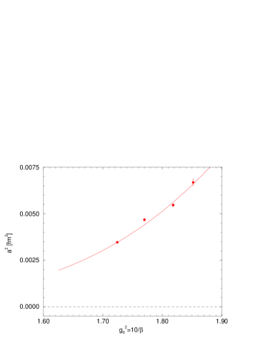
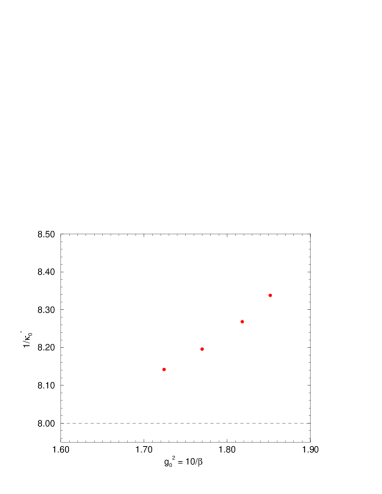
Figure 5: Left panel: $a^{2}$ versus $g_{0}^{2}$. The curve is from the running coupling constant, using the $2$-loop beta function normalised to the $\beta=5.80$ result. Right panel: $1/\kappa_{0}^{*}$ versus $g_{0}^{2}$. The horizontal dashed lines represents the value in the continuum limit.

The curve is the running coupling constant, $g_{0}^{2}=10/\beta$ using the $2$-loop QCD beta function, normalised to $\beta=5.80$, namely

$${a^{2}(\beta)\over a^{2}(\beta_{0})}=\left({\beta_{0}\over\beta}\right)^{-{b_{1}\over b_{0}^{2}}}\,\exp\left({-{1\over 10b_{0}}\,(\beta-\beta_{0})}\right)\,,\qquad\beta_{0}=5.80\,,$$ (15)

($b_{0}$, $b_{1}$ are the first two coefficients of the beta function). There seems to be reasonable agreement between the data points and the curve. The right hand panel of Fig. 5 indicates how the initial point, $\kappa_{0}^{*}$, on the $SU(3)$ flavour symmetric line changes with $g_{0}^{2}$.

3 Conclusions

Our programme is to tune strange and light quark masses to their physical values simultaneously by keeping $\overline{m}=1/3\,(2m_{l}+m_{s})=\mbox{const.}$. As the light quark mass is decreased then $M_{\pi}\searrow$ and $M_{K}\nearrow$. Singlet quantities, here denoted by $X_{S}(\kappa_{0})$ remain constant starting from a point on the $SU(3)$ flavour symmetric line — the Gell-Mann–Okubo result. We can use this result and $X_{S}^{\exp}$ to determine the $a_{S}(\kappa_{0})$ scale. Varying $\kappa_{0}$ – determines when pairs of singlet quantities such as $(X_{\pi},X_{N})$ and $(X_{\pi},X_{\rho})$ cross giving a common lattice spacing $a$. By arranging so that $X_{t_{0}}$, $X_{w_{0}}$ also cross here, we are able to give a determination of the ‘secondary’ scales $\sqrt{t_{0}^{\exp}}$ and $w_{0}^{\exp}$ $[\mbox{fm}]$. Finally in Fig. 6 a comparison with other results is given.

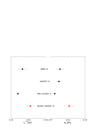
Figure 6: $\sqrt{t_{0}^{\exp}}$, left plot and $w_{0}^{\exp}$, right plot in fm for BMW 12 [5], HotQCD 14 [8], RBC-UKQCD 14 [9], together with the present results.

References

[1]
V. G. Bornyakov et al. [QCDSF–UKQCD Collaboration],
arXiv:1508.05916[hep-lat].
[2]
W. Bietenholz et al. [QCDSF–UKQCD Collaboration],
Phys. Lett. B690 (2010) 436,
[arXiv:1003.1114[hep-lat]].
[3]
W. Bietenholz et al. [QCDSF–UKQCD Collaboration],
Phys. Rev. D84 (2011) 054509,
[arXiv:1102.5300[hep-lat]].
[4]
M. Lüscher,
JHEP 1008 (2010) 071,
[arXiv:1006.4518[hep-lat]].
[5]
S. Borsanyi et al. [BMW Collaboration],
JHEP 010 (2012) 1209,
[arXiv:1203.4469[hep-lat]].
[6]
O. Bär et al.
Phys. Rev. D89 (2014) 034505,
[arXiv:1312.4999[hep-lat]].
[7]
N. Cundy et al. [QCDSF–UKQCD Collaboration],
Phys. Rev. D79 (2009) 094507,
[arXiv:0901.3302[hep-lat]].
[8]
A. Bazavov et al. [HotQCD Collaboration],
Phys. Rev. D90 (2014) 094503,
[arXiv:1407.6387[hep-lat]].
[9]
T. Blum et al. [RBC–UKQCD Collaborations],
arXiv:1411.7017[hep-lat].
[10]
Y. Nakamura et al.,
Proc. Sci. Lattice 2010 (2010) 040,
arXiv:1011.0199[hep-lat].
[11]
R. G. Edwards et al.,
Nucl. Phys. Proc. Suppl. 140 (2005) 832,
arXiv:hep-lat/0409003.