Disorder-promoted $C_{4}$-symmetric magnetic order in iron-based superconductors

Abstract

In most iron-based superconductors, the transition to the magnetically ordered state is closely linked to a lowering of structural symmetry from tetragonal ($C_{4}$) to orthorhombic ($C_{2}$). However, recently, a regime of $C_{4}$-symmetric magnetic order has been reported in certain hole-doped iron-based superconductors. This novel magnetic ground state can be understood as a double-Q spin density wave characterized by two order parameters $\boldsymbol{\mathbf{M}}_{1}$ and $\boldsymbol{\mathbf{M}}_{2}$ related to each of the two $\mathbf{Q}$ vectors. Depending on the relative orientations of the order parameters, either a noncollinear spin-vortex crystal or a nonuniform charge-spin density wave could form. Experimentally, Mössbauer spectroscopy, neutron scattering, and muon spin rotation established the latter as the magnetic configuration of some of these optimally hole-doped iron-based superconductors. Theoretically, low-energy itinerant models do support a transition from single-Q to double-Q magnetic order, but with nearly-degenerate spin-vortex crystal and charge-spin density wave states. In fact, extensions of these low-energy models including additional electronic interactions tip the balance in favor of the spin-vortex crystal, in apparent contradiction with the recent experimental findings. In this paper, we revisit the phase diagram of magnetic ground states of low-energy multi-band models in the presence of weak disorder. We show that impurity scattering not only promotes the transition from $C_{2}$ to $C_{4}$-magnetic order, but it also favors the charge-spin density wave over the spin-vortex crystal phase. Additionally, in the single-Q phase, our analysis of the nematic coupling constant in the presence of disorder supports the experimental finding that the splitting between the structural and stripe-magnetic transition is enhanced by disorder.

I Introduction

One of the common features of iron-based superconductors (FeSC) is the emergence of superconductivity in close proximity to a magnetic instability. Paglione and Greene (2010); Andrey V. Chubukov and Peter J. Hirschfeld (2015) Even more intriguingly, superconductivity coexists with magnetism in some of the iron-based compounds. Pratt et al. (2009); Laplace et al. (2009) Thus it is imperative to study the nature of the magnetic order in the FeSC compounds in order to better understand the superconducting state in these materials.

Most of the undoped compounds of the FeSC family exhibit magnetic stripe order with the spins on the iron sites lying in the planes and being aligned ferromagnetically along one direction, and antiferromagnetically along the other. In addition to the continuous $O(3)$ spin-rotational symmetry broken below the magnetic transition temperature $T_{\mathrm{N}}$, this stripe-magnetic (SM) state also breaks an additional $\mathbb{Z}_{2}$ Ising-like symmetry since the ordering vector of the spin-density wave (SDW) $\boldsymbol{\mathbf{S}}(\boldsymbol{\mathbf{r}})=\boldsymbol{\mathbf{M}}\mathrm{e}^{\mathrm{i}\boldsymbol{\mathbf{Q}}\cdot\boldsymbol{\mathbf{r}}}$ is either $\boldsymbol{\mathbf{Q}}=(0,\pi)$ or $\boldsymbol{\mathbf{Q}}=(\pi,0)$. The $\mathbb{Z}_{2}$ (or, equivalently, $C_{2}$) symmetry breaking can occur at temperatures $T_{\mathrm{s}}>T_{\mathrm{N}}$ and entails a structural transition from tetragonal ($C_{4}$) to orthorhombic ($C_{2}$). Furthermore, if the transitions are split, this allows for an intermediate phase with broken $\mathbb{Z}_{2}$ symmetry but no magnetic long-range order. This intermediate phase is dubbed nematic order Fang et al. (2008); Xu et al. (2008); R. M. Fernandes et al. (2014). Interestingly, the splitting $\Delta T=T_{\mathrm{s}}-T_{\mathrm{N}}$ between the two transitions, and the stabilization of an intermediate nematic phase, depends on disorder. Jesche et al. (2010); Takasada Shibauchi ; Liang et al. (2015). Uncovering the origin of the nematic phase – either a spin-driven or an orbital-driven mechanism – may also elucidate the mechanism for superconductivity.

Recently, $C_{4}$-magnetic phases have been observed in the hole-doped compounds Ba(Fe_1-xMn_x)₂As₂, Kim et al. (2010) Ba_1-xNa_xFe₂As₂, Avci S. et al. (2014), Ba_1-xK_xFe₂As₂, Hassinger et al. (2012); Böhmer A. E. et al. (2015); Allred et al. (2015) and Sr_1-xK_xFe₂As₂ J. M. Allred et al. , suggesting that such phases might be a general feature in the phase diagram of hole-doped FeSC Wang et al. (2015). The magnetic Bragg peaks of these $C_{4}$-magnetic phases occur at the same momenta $\boldsymbol{\mathbf{Q}}_{1}=(\pi,0)$ and $\boldsymbol{\mathbf{Q}}_{2}=(0,\pi)$ as in the stripe-ordered state and, consequently, such a state can be understood as the superposition of two spin-density waves $\boldsymbol{\mathbf{S}}(\boldsymbol{\mathbf{r}})=\boldsymbol{\mathbf{M}}_{1}\mathrm{e}^{\mathrm{i}\boldsymbol{\mathbf{Q}}_{1}\cdot\boldsymbol{\mathbf{r}}}+\boldsymbol{\mathbf{M}}_{2}\mathrm{e}^{\mathrm{i}\boldsymbol{\mathbf{Q}}_{2}\cdot\boldsymbol{\mathbf{r}}}$, i. e. a double-Q SDW, as illustrated in Fig. 1. As in the case of stripe antiferromagnetism, which is preceded by nematic order, also these double-Q magnetic states can in principle be melted in two stages, passing through an intermediate state of vestigial charge or chiral order. R. M. Fernandes et al. (2015)

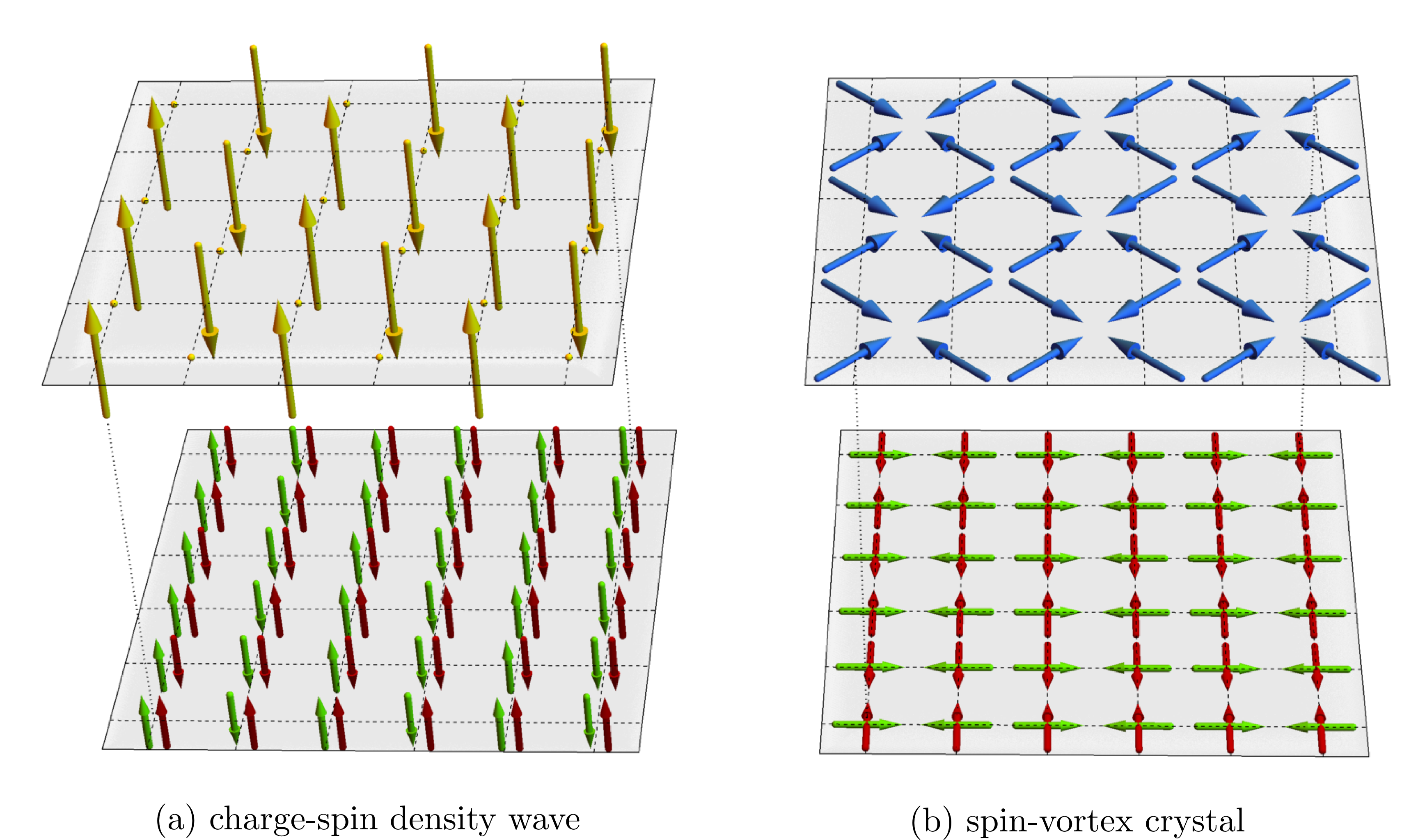
Figure 1: Illustration of the two double-$\boldsymbol{\mathbf{Q}}$ magnetically ordered states as a superposition of two single-$\boldsymbol{\mathbf{Q}}$ stripe-magnetic states. (a) Aligning the order parameters $\boldsymbol{\mathbf{M}}_{1}=\pm\boldsymbol{\mathbf{M}}_{2}$ (anti)parallel yields a charge-spin density wave. This order is favorable if $g<|w|$ and $w<0$. (b) Aligning the order parameters $\boldsymbol{\mathbf{M}}_{1}\perp\boldsymbol{\mathbf{M}}_{2}$ perpendicular to each other leads to the formation of a spin-vortex crystal. This state is favorable if $g<0$ and $w>0$. Otherwise, single-$\boldsymbol{\mathbf{Q}}$ stripe order is favored.

The existence of double-$\boldsymbol{\mathbf{Q}}$ magnetic states as additional ground states for the FeSC has also been established by different theoretical approaches, Lorenzana et al. (2008); Eremin and Chubukov (2010); Kang and Tešanović (2011); Gianluca Giovannetti et al. (2011); Brydon et al. (2011); Fernandes et al. (2012a); Cvetkovic and Vafek (2013); Kang et al. (2015); Gastiasoro and Andersen (2015) all of which suggest the two possible double-$\boldsymbol{\mathbf{Q}}$ ground states visualized in Fig. 1 in addition to the single-$\boldsymbol{\mathbf{Q}}$ stripe-magnetic order. Fig. 1(a) shows the charge-spin density wave (CSDW) that arises from aligning $\boldsymbol{\mathbf{M}}_{1}$ and $\boldsymbol{\mathbf{M}}_{2}$ either parallel or antiparallel. This results in a nonuniform magnetization with vanishing average moment at the even lattice sites and staggered-like order at the odd lattice sites, or vice versa. If $\boldsymbol{\mathbf{M}}_{1}$ and $\boldsymbol{\mathbf{M}}_{2}$ are orthogonal, the resulting spin-vortex crystal (SVC) is characterized by a noncollinear magnetization that is illustrated in Fig. 1(b).

All three magnetic states, the stripe-magnetic and the two double-$\boldsymbol{\mathbf{Q}}$ magnetic states, can be rationalized in terms of a Ginzburg-Landau expansion of the free energy in terms of the two magnetic order parameters $\boldsymbol{\mathbf{M}}_{i}$ Fernandes et al. (2012a); Wang and Fernandes (2014); R. M. Fernandes et al. (2015),

$$F[\boldsymbol{\mathbf{M}}_{i}] =a\left(\boldsymbol{\mathbf{M}}_{1}^{2}+\boldsymbol{\mathbf{M}}_{2}^{2}\right)+\frac{u}{2}\left(\boldsymbol{\mathbf{M}}_{1}^{2}+\boldsymbol{\mathbf{M}}_{2}^{2}\right)^{2}$$

$$\qquad-\frac{g}{2}\left(\boldsymbol{\mathbf{M}}_{1}^{2}-\boldsymbol{\mathbf{M}}_{2}^{2}\right)^{2}+2w\left(\boldsymbol{\mathbf{M}}_{1}\cdot\boldsymbol{\mathbf{M}}_{2}\right)^{2}~{}.$$ (1)

Depending on the quartic coefficients $u$, $g$, and $w$, the corresponding energy is minimized by one of the three magnetic ground states described above, provided that $u>\max(0,g,-w)$.

For $g>\max(0,-w)$, the stripe-ordered $C_{2}$-magnetic phase is the magnetic ground state of systems described by the free energy ((1)), and it is accompanied by a structural transition from tetragonal to orthorhombic. This scenario is supported by itinerant as well as by localized approaches to magnetism in FeSC, and it is experimentally well established that stripe-SDW is the magnetic ground state of many compounds of this family of materials. If, on the other hand, $g<\max(0,-w)$, one of the two above described possibilities of $C_{4}$-magnetic phases is realized, depending on whether $w>0$ (leading to a spin vortex crystal) or $w<0$ (implying a charge-spin density wave).

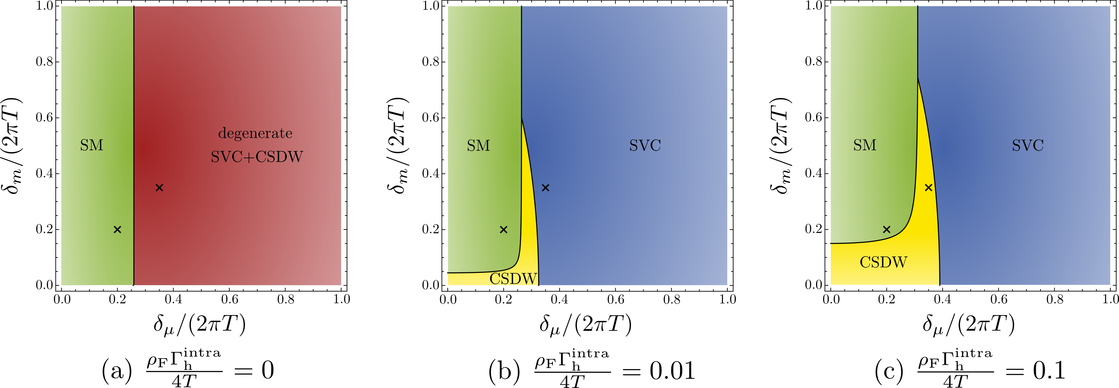
Figure 2: Evolution of the phase diagrams, as function of increasing scattering rate, of the possible magnetic ground states of our three-band minimal model of iron-based superconductors. Here we used $\Gamma_{\mathrm{e-e}}^{\mathrm{inter}}=0.1\Gamma_{\mathrm{h}}^{\mathrm{intra}}$, and the phase diagrams are obtained in the limit $\delta_{\mu}\ll 2\pi T$ and $\delta_{m}\ll 2\pi T$. The regime of single-Q stripe order (SM) is shown in green, the double-Q spin-vortex crystal (SVC) order is indicated by blue, and the yellow region represents the double-Q charge-spin density wave (CSDW). In the clean regime, where all scattering rates are zero, SVC and CSDW order are degenerate and we indicated this region with $w=0$ in red. The crosses mark the points in the phase diagram at which we plotted $g$ and $w$ as a function of scattering rate in Fig. 5 and Fig. 7, respectively.

Experimentally, several probes J. M. Allred et al. ; Waßer et al. (2015); Mallett et al. (2015) established that the magnetic moments in the $C_{4}$-magnetic phase observed in hole-doped FeSC are aligned parallel to the $c$ axis, i. e., pointing out of plane, and that the magnetic moment vanishes at every second lattice site while it is doubled at the others. These features uniquely identify this $C_{4}$-magnetic phase as a realization of a charge-spin density wave, corresponding to $w<0$. Therefore, it is important to elucidate theoretically which generic features of low-energy models yield $w<0$ and $g<|w|$.

Localized approaches based on the $J_{1}$-$J_{2}$ Heisenberg model favor the single-$\boldsymbol{\mathbf{Q}}$ stripe-ordered state, Chandra et al. (1990) whereas itinerant approaches allow for both signs of $g$. Focusing on the three-band itinerant low-energy model previously employed in the literature Eremin and Chubukov (2010); Fernandes et al. (2012a); Wang et al. (2015), one finds a sign-change from $g>0$ near perfect nesting to $g<0$ away from perfect nesting, implying a transition from single-Q to a double-$\boldsymbol{\mathbf{Q}}$ state. However, due to phase space restrictions, this same model generically gives $w=0$ (for details, see Sect. II.1), leaving the noncollinear SVC and the nonuniform CSDW order degenerate (see Fig. 2(a)). Extensions of this model tend to favor $w>0$, in disagreement with the recent experiments – this is indeed obtained by including residual electronic interactionsEremin and Chubukov (2010); Wang et al. (2015) or, as we will show below, an incipient fourth pocket. We note that although Ref. Wang and Fernandes, 2014 proposed that the proximity to a Néel-like state can favor $w<0$, this scenario is only applicable to Ba(Fe_1-xMn_x)₂As₂, since the compound BaMn₂As₂ displays Néel order – which is not the case for Ba_1-xNa_xFe₂As₂ or Ba_1-xK_xFe₂As₂. Note also that Ref. Morten H. Christensen et al., showed that the spin-orbit coupling leads to anisotropic quadratic terms in the free energy (1) that favor the CSDW order, even though $w=0$. This however only works near the magnetic transition, since at low temperatures the quartic terms are the ones that determine the ground state.

Therefore, understanding which additional features can lead to $w<0$ is essential to shed light on the mechanisms behind the formation of the $C_{4}$ phase. Since charged potential impurities can locally stabilize charge-spin density wave order, Lorenzana et al. (2008); Gastiasoro and Andersen (2015) one promising approach is the inclusion of doping effects beyond a rigid-band model. In this paper, we consider the effect of impurity scattering on the quartic coupling constants $g$ and $w$ of the itinerant minimal three-band model. We find that, in the regime where $g>0$ in the clean system, the inclusion of disorder suppresses $g$, and may even change its sign. One of the consequences of this result is that the splitting $\Delta T=T_{\mathrm{s}}-T_{\mathrm{N}}$ between the structural and magnetic transitions to the stripe-ordered state may, depending on the vicinity of the system to a tricritical point, enhance upon increasing disorder, in agreement with recent experiments on BaFe₂As₂ subject to electron irradiation Takasada Shibauchi . Furthermore, disorder itself may cause a transition from single-Q to double-Q order near perfect nesting, as shown in Figs. 2(b) and (c). Our most important result, however, is the fate of the vanishing coefficient $w$ in the presence of disorder. We find that disorder generally lifts the degeneracy between CSDW and SVC, favoring $w<0$ (and therefore CSDW) near perfect nesting (Figs. 2(b) and (c)). Consequently, this opens the interesting possibility of controlling the magnetic ground state in FeSC with controlled disorder introduced via irradiation or removed via annealing.

The paper is structured as follows. Section II introduces the microscopic model including disorder, which we use to calculate the free energy. We start by recapitulating that $w=0$ follows immediately from a three-band model in Section II.1, followed by the discussion of a fourth band in Section II.2 which only allows for $w>0$. Consequently, we study the effect of disorder as an alternative route and show in section II.3 that the presence of impurities can indeed render $w<0$ already within the simpler three-band model. The nature of the magnetic ground state is determined by the coefficients $g$ and $w$, and their dependence on disorder is discussed in Section III, also elucidating the disorder dependence of the splitting between nematic and magnetic transition. Finally, we combine our results to obtain a phase diagram of magnetic ground states in the presence of disorder, which complements the discussion of our conclusions in Section IV.

II Microscopic model

We consider a minimal multi-band modelEremin and Chubukov (2010); Fernandes et al. (2012a) for iron-based superconductors (FeSC) consisting of two circular hole pockets centered around the $\Gamma$ point and the $M$ point of the Fe-only Brillouin zone, i. e. around $(0,0)$ and $(\pi,\pi)$, respectively, and two elliptical electron pockets centered around $X$ and $Y$ at $\boldsymbol{\mathbf{Q}}_{1}=(\pi,0)$ and $\boldsymbol{\mathbf{Q}}_{2}=(0,\pi)$, respectively. The pocket at the $M$ point however is not a generic feature of this class of materials since it exists only in some of the iron-based compounds. Moreover, even in the compounds in which the pocket at the $M$ point exists, this band is not guaranteed to cross the Fermi level for all values of $k_{z}$. Our analysis in section II.2 will show that the presence of such an incipient hole pocket at the $M$ point cannot explain the formation of a charge-spin density wave and hence can be neglected in the remainder of this paper. The noninteracting part of the model is described by the Hamiltonian

$$\mathcal{H}_{0}=\sum_{\boldsymbol{\mathbf{k}},\sigma,\lambda}\varepsilon_{\lambda,\boldsymbol{\mathbf{k}}}c_{\lambda,\boldsymbol{\mathbf{k}},\sigma}^{\dagger}c_{\lambda,\boldsymbol{\mathbf{k}},\sigma}~{},$$ (2)

where the fact that the bands are centered around different momenta is reflected in the band index $\lambda\in\{\mathrm{h}_{\Gamma},\mathrm{h}_{M},\mathrm{e}_{1},\mathrm{e}_{2}\}$ where the hole bands are labeled by $\mathrm{h}_{\Gamma}$ and $\mathrm{h}_{M}$, and the electron bands by $\mathrm{e}_{1}\equiv\mathrm{e}_{X}$ and $\mathrm{e}_{2}\equiv\mathrm{e}_{Y}$. Thus $c_{\lambda,\boldsymbol{\mathbf{k}},\sigma}^{\dagger}$ creates an electron in band $\lambda$ with spin $\sigma$, and the respective dispersions near the Fermi energy can be parametrized as follows

$$\begin{split}&\varepsilon_{\mathrm{h}_{\Gamma},\boldsymbol{\mathbf{k}}}=-\varepsilon_{\boldsymbol{\mathbf{k}}}~{},\\ &\varepsilon_{\textrm{e}_{1},\boldsymbol{\mathbf{k}}}=\varepsilon_{\boldsymbol{\mathbf{k}}}-\delta_{\mu}+\delta_{m}\cos(2\theta)~{},\\ &\varepsilon_{\textrm{e}_{2},\boldsymbol{\mathbf{k}}}=\varepsilon_{\boldsymbol{\mathbf{k}}}-\delta_{\mu}-\delta_{m}\cos(2\theta)~{},\\ &\varepsilon_{\mathrm{h}_{M},\boldsymbol{\mathbf{k}}}=-\varepsilon_{\boldsymbol{\mathbf{k}}}-E_{M}~{},\end{split}$$ (3)

with $\varepsilon_{\boldsymbol{\mathbf{k}}}=\frac{k^{2}}{2m}-\varepsilon_{0}+\mu$ and $\theta=\arctan(k_{y}/k_{x})$. $\delta_{\mu}$ characterizes the shift of the chemical potential and is therefore proportional to doping, and $\delta_{m}$ is a measure of the ellipticity of the electron bands. The top of the hole band at the $M$ point is lower in energy than the top of the hole band at the $\Gamma$ point, i.e. $E_{M}>0$, such that it is not guaranteed to cross the Fermi surface even if it does exist. Note that $E_{M}=\delta_{\mu}=\delta_{m}=0$ gives perfectly nested electron and hole bands. The respective noninteracting single-particle Green’s functions are given by $G_{\lambda,\boldsymbol{\mathbf{k}}}(\nu_{n})=(\mathrm{i}\nu_{n}-\varepsilon_{\lambda,\boldsymbol{\mathbf{k}}})^{-1}$ with $\nu_{n}=2\pi T(n+1/2)$ being a fermionic Matsubara frequency.

Since we are concerned with the nature of the magnetically ordered state, we focus on the electron-electron interaction projected in the spin channel, hereafter denoted by $V$. Upon performing a Hubbard-Stratonovich transformation, two magnetic order parameters arise, $\boldsymbol{\mathbf{M}}_{1}$ and $\boldsymbol{\mathbf{M}}_{2}$, associated with the two ordering vectors $\boldsymbol{\mathbf{Q}}_{1}=(\pi,0)$ and $\boldsymbol{\mathbf{Q}}_{2}=(0,\pi)$, respectively. Their coupling to the electronic degrees of freedom is given by

$$\mathcal{H}_{\mathrm{int}} =-\sum_{\boldsymbol{\mathbf{k}},i}\boldsymbol{\mathbf{M}}_{i}\cdot\left(c_{\mathrm{h}_{\Gamma},\boldsymbol{\mathbf{k}},\sigma_{1}}^{\dagger}\boldsymbol{\mathbf{\sigma}}_{\sigma_{1},\sigma_{2}}c_{\mathrm{e}_{i},\boldsymbol{\mathbf{k}},\sigma_{2}}+\mathrm{h.\,c.}\right)$$

$$\qquad-\sum_{\boldsymbol{\mathbf{k}},i}\boldsymbol{\mathbf{M}}_{i}\cdot\left(c_{\mathrm{h}_{M},\boldsymbol{\mathbf{k}},\sigma_{1}}^{\dagger}\boldsymbol{\mathbf{\sigma}}_{\sigma_{1},\sigma_{2}}c_{\mathrm{e}_{\bar{i}},\boldsymbol{\mathbf{k}},\sigma_{2}}+\mathrm{h.\,c.}\right)$$ (4)

where $\bar{i}=2,1$ if $i=1,2$. In the vicinity of the magnetic phase transition, we can integrate out the electronic degrees of freedom and derive the free energy expansion of the system

$$F[\boldsymbol{\mathbf{M}}_{i}] =\sum_{i}a_{i}|\boldsymbol{\mathbf{M}}_{i}|^{2}+\sum_{i,j}u_{ij}|\boldsymbol{\mathbf{M}}_{i}|^{2}|\boldsymbol{\mathbf{M}}_{j}|^{2}$$

$$\qquad+2w(\boldsymbol{\mathbf{M}}_{1}\cdot\boldsymbol{\mathbf{M}}_{2})^{2}~{},$$ (5)

where the coefficients $a_{i}$, $u_{ij}$ and $w$ can be calculated from the microscopic model introduced above. Due to the rotational symmetry connecting the electron bands, it holds that $a_{1}=a_{2}$, $u_{11}=u_{22}$, and $u_{12}=u_{21}$. The free energy (5) can be brought to the form of Eq. (1) using $u\equiv u_{12}+u_{11}$ and $g\equiv u_{12}-u_{11}$.

While the transition temperature is determined by the vanishing of the quadratic coefficient, the nature of the magnetic ground state is solely determined by the interplay of the quartic coefficients $g$ and $w$ in this expansion as long as $u>\max(0,g,-w)$. Since our goal is to explain the formation of charge-spin density waves in a low-energy model of the FeSC, we are mainly interested in scenarios that yield $w<0$. In the remainder of this section, we show that neglecting the incipient hole pocket at $M$ yields $w=0$ in the clean case as a consequence of phase space restrictions. However, including the incipient pocket in a clean model leads to $w>0$ and thus the spin-vortex crystal would be favorable. Only the inclusion of disorder can yield $w<0$ and thus render the nonuniform charge-spin density wave order favorable

II.1 Clean three-band model

We start our considerations with the clean three-band model, i. e., disregarding the second hole pocket at the $M$ point which is not present in all FeSC compounds. The coefficients in the expansion of the free energy, previously defined in Ref. Fernandes et al., 2012a, are given by:

$$a_{i} =\frac{2}{V}+2\int_{k}G_{\mathrm{h}_{\Gamma},\boldsymbol{\mathbf{k}}}(\nu_{n})G_{\mathrm{e}_{i},\boldsymbol{\mathbf{k}}}(\nu_{n})~{},$$

$$u =\frac{1}{2}\int_{k}G_{\mathrm{h}_{\Gamma},\boldsymbol{\mathbf{k}}}^{2}(\nu_{n})[G_{\mathrm{e}_{1},\boldsymbol{\mathbf{k}}}(\nu_{n})+G_{\mathrm{e}_{2},\boldsymbol{\mathbf{k}}}(\nu_{n})]^{2}~{},$$

$$g =-\frac{1}{2}\int_{k}G_{\mathrm{h}_{\Gamma},\boldsymbol{\mathbf{k}}}^{2}(\nu_{n})[G_{\mathrm{e}_{1},\boldsymbol{\mathbf{k}}}(\nu_{n})-G_{\mathrm{e}_{2},\boldsymbol{\mathbf{k}}}(\nu_{n})]^{2}~{},$$

$$w =0~{},$$ (6)

where we abbreviated $\int_{k}\ldots\equiv T\sum_{n}\int\frac{\mathrm{d}\boldsymbol{\mathbf{k}}}{(2\pi)^{2}}\ldots$ For convenience, we write $u$ and $g$ here in the symmetrized form, namely $u=\tfrac{1}{2}(u_{11}+u_{12}+u_{21}+u_{22})$ and $g=-\tfrac{1}{2}(u_{11}-u_{12}-u_{21}+u_{22})$. The coefficient $w$ vanishes in the clean model as a consequence of the trace in spin space Morten H. Christensen et al. : The most generic quartic diagram [see Fig. 3(a)] is proportional to

$$\operatorname{tr}\bigg{[}\sum_{ijkl}M_{\lambda_{1}}^{(i)}\sigma_{i}M_{\lambda_{2}}^{(j)}\sigma_{j}M_{\lambda_{3}}^{(k)}\sigma_{k}M_{\lambda_{4}}^{(l)}\sigma_{l}\bigg{]}$$

$$=2\big{[}(\boldsymbol{\mathbf{M}}_{\lambda_{1}}\cdot\boldsymbol{\mathbf{M}}_{\lambda_{2}})(\boldsymbol{\mathbf{M}}_{\lambda_{3}}\cdot\boldsymbol{\mathbf{M}}_{\lambda_{4}})$$

$$\qquad-(\boldsymbol{\mathbf{M}}_{\lambda_{1}}\cdot\boldsymbol{\mathbf{M}}_{\lambda_{3}})(\boldsymbol{\mathbf{M}}_{\lambda_{2}}\cdot\boldsymbol{\mathbf{M}}_{\lambda_{4}})$$

$$\qquad+(\boldsymbol{\mathbf{M}}_{\lambda_{1}}\cdot\boldsymbol{\mathbf{M}}_{\lambda_{4}})(\boldsymbol{\mathbf{M}}_{\lambda_{2}}\cdot\boldsymbol{\mathbf{M}}_{\lambda_{3}})\big{]}~{}.$$ (7)

Within the minimal model, introduced in Eqs. (2) and (4), and with the additional simplification of neglecting the pocket at the $M$ point, the absence of scattering as well as interactions between the electron bands require that either $\lambda_{1}=\lambda_{2}$ and $\lambda_{3}=\lambda_{4}$, or $\lambda_{1}=\lambda_{4}$ and $\lambda_{2}=\lambda_{3}$ holds, as can be seen from Fig. 3(a). Both conditions result in $\operatorname{tr}[(\boldsymbol{\mathbf{M}}_{\lambda_{1}}\cdot\boldsymbol{\mathbf{\sigma}})(\boldsymbol{\mathbf{M}}_{\lambda_{2}}\cdot\boldsymbol{\mathbf{\sigma}})(\boldsymbol{\mathbf{M}}_{\lambda_{3}}\cdot\boldsymbol{\mathbf{\sigma}})(\boldsymbol{\mathbf{M}}_{\lambda_{4}}\cdot\boldsymbol{\mathbf{\sigma}})]=2|\boldsymbol{\mathbf{M}}_{\lambda_{1}}|^{2}|\boldsymbol{\mathbf{M}}_{\lambda_{3}}|^{2}$ and thus imply $w=0$ in the clean case. On the contrary, the inclusion of interband scattering or interactions between the two electron pockets at $\boldsymbol{\mathbf{Q}}_{1}$ and $\boldsymbol{\mathbf{Q}}_{2}$ allows for contributions where $\lambda_{1}=\lambda_{3}$ and $\lambda_{2}=\lambda_{4}$, rendering $w$ finite since then $\operatorname{tr}[(\boldsymbol{\mathbf{M}}_{\lambda_{1}}\cdot\boldsymbol{\mathbf{\sigma}})(\boldsymbol{\mathbf{M}}_{\lambda_{2}}\cdot\boldsymbol{\mathbf{\sigma}})(\boldsymbol{\mathbf{M}}_{\lambda_{3}}\cdot\boldsymbol{\mathbf{\sigma}})(\boldsymbol{\mathbf{M}}_{\lambda_{4}}\cdot\boldsymbol{\mathbf{\sigma}})]=2\left[2(\boldsymbol{\mathbf{M}}_{\lambda_{1}}\cdot\boldsymbol{\mathbf{M}}_{\lambda_{2}})-|\boldsymbol{\mathbf{M}}_{\lambda_{1}}|^{2}|\boldsymbol{\mathbf{M}}_{\lambda_{2}}|^{2}\right]$.

Figure 3: Diagrams in the absence of disorder. (a) Sketch of a generic quartic diagram before performing the spin trace: Each vertex couples the hole band to one of the electron bands, and the dashed lines indicate that scattering or additional interactions could alter the diagram. (b) Contribution to the planar coupling constant $w$ if the incipient hole pocket at $M$ is taken into account.

II.2 Incipient hole pocket at the $M$ point

The inclusion of an incipient hole pocket at $(\pi,\pi)$ allows for contributions that render $w$ finite in an analogous manner. The contribution to the planar coupling $w$ that survives the spin trace as a consequence of the presence of the second hole pocket is depicted diagrammatically in Fig. 3(b). We consider the simplest case where $\delta_{\mu}=0=\delta_{m}$, i. e., perfect nesting of the hole band at the $\Gamma$ point and the two electron bands, since this yields a finite value for the planar coupling,

$$w =4\int_{k}G_{\mathrm{h}_{\Gamma},\boldsymbol{\mathbf{k}}}(\nu_{n})G_{\mathrm{e}_{1},\boldsymbol{\mathbf{k}}}(\nu_{n})G_{\mathrm{h}_{M},\boldsymbol{\mathbf{k}}}(\nu_{n})G_{\mathrm{e}_{2},\boldsymbol{\mathbf{k}}}(\nu_{n})$$

$$=4T\sum_{n=-\infty}^{\infty}\rho_{\mathrm{F}}\int_{-\infty}^{\infty}\mathrm{d}\epsilon\,\frac{1}{\mathrm{i}\nu_{n}+\epsilon}\frac{1}{\mathrm{i}\nu_{n}+\epsilon+E_{M}}\frac{1}{(\mathrm{i}\nu_{n}-\epsilon)^{2}}$$

$$\approx\left\{\begin{matrix}\frac{7\rho_{\mathrm{F}}\zeta(3)}{2\pi^{2}T^{2}}\approx 0.43\frac{\rho_{\mathrm{F}}}{T^{2}}&~{},\qquad E_{M}\ll T~{},\\ \frac{4\rho_{\mathrm{F}}}{E_{M}^{2}}&~{},\qquad E_{M}\gg T~{},\end{matrix}\right.$$ (8)

where $\zeta(z)$ is the Riemann zeta function, and we assumed the density of states at the Fermi level to be given by a constant $\rho_{\mathrm{F}}$ in all bands.

Hence we find that the inclusion of the second hole pocket indeed lifts the degeneracy of the two double-Q magnetically ordered states. However, it can only account for the formation of a spin-vortex crystal since $w>0$ always. Furthermore, if the pocket at $M$ is shifted to energies far below the Fermi level, we reproduce the results of the previously discussed three-band model since the coefficient $w$ vanishes in the limit $E_{M}\rightarrow\infty$, which is the relevant limit for many of the FeSC compounds.

A positive planar coupling $w>0$ has also been obtained in previous studies of other extensions of the clean three-band model such as the perturbative inclusion of additional interactions. Eremin and Chubukov (2010); Wang et al. (2015) This suggests a different route to $w<0$ is needed in order to explain the formation of the collinear CSDW state within this low-energy model. In the remainder of this paper, we investigate the effect of disorder on the magnetic ground state. Furthermore, we neglect the hole pocket at the $M$ point since it is not a generic feature of the FeSC family and its inclusion is not able to explain why the nonuniform CSDW is favored over the noncollinear SVC in the hole-doped compounds.

II.3 Impurity scattering

Impurity scattering will affect both the magnetic transition temperature, determined by the vanishing of $a_{i}$, and the nature of the magnetic ground state, determined by $g$ and $w$. Hereafter, we focus on the latter effect – the former gives rise to a suppression of the magnetic transition temperature with disorder, as shown elsewhere Fernandes et al. (2012b); Liang et al. (2015). In the particle-hole symmetric case (perfect nesting), where $\delta_{\mu}=\delta_{m}=0$, the nematic coupling constant $g$ vanishes. Finite ellipticity $\delta_{m}\neq 0$, however, causes $g$ to be finite. The effect of doping can then partially be accounted for by a finite value of the chemical potential, i. e., $\delta_{\mu}\neq 0$.

Meanwhile, doping also introduces disorder, which has a different effect on the electronic structure than the rigid band shift assumed by changing the chemical potential.Wadati et al. (2010) For instance, it has been shown that impurity scattering can locally stabilize charge-spin density wave order,Gastiasoro and Andersen (2015) thus suggesting that the inclusion of disorder for the itinerant electrons participating in the formation of the magnetically ordered state is an important ingredient for the investigation of the CSDW state. Hence we consider an arbitrary realization of nonmagnetic impurities, thus adding the term

$$\mathcal{H}_{\mathrm{dis}}=\sum_{\lambda,\lambda^{\prime}}\sum_{\boldsymbol{\mathbf{k}},\boldsymbol{\mathbf{k}}^{\prime}}\sum_{\sigma}\,c_{\lambda,\boldsymbol{\mathbf{k}},\sigma}^{\dagger}W_{\lambda\lambda^{\prime}}(\boldsymbol{\mathbf{k}},\boldsymbol{\mathbf{k}}^{\prime})c_{\lambda^{\prime},\boldsymbol{\mathbf{k}}^{\prime},\sigma}$$ (9)

to the Hamiltonian. As usual, we are not interested in quantities that depend on the microscopic disorder realization, but rather in self-averaged physical observables. Therefore, we are interested in disorder-averaged quantities where all information about the disorder is encoded in the correlation function

$$\left<W_{\lambda_{1}\lambda_{1}^{\prime}}(\boldsymbol{\mathbf{k}}_{1},\boldsymbol{\mathbf{k}}_{1}^{\prime})W_{\lambda_{2}\lambda_{2}^{\prime}}(\boldsymbol{\mathbf{k}}_{2},\boldsymbol{\mathbf{k}}_{2}^{\prime})\right>_{\mathrm{dis}}$$ (10)

$$=\Gamma_{\lambda_{1}\lambda_{1}^{\prime}\lambda_{2}\lambda_{2}^{\prime}}(\boldsymbol{\mathbf{k}}_{1},\boldsymbol{\mathbf{k}}_{1}^{\prime},\boldsymbol{\mathbf{k}}_{2},\boldsymbol{\mathbf{k}}_{2}^{\prime})\updelta(\boldsymbol{\mathbf{k}}_{1}+\boldsymbol{\mathbf{k}}_{2}-\boldsymbol{\mathbf{k}}_{1}^{\prime}-\boldsymbol{\mathbf{k}}_{2}^{\prime}+\boldsymbol{\mathbf{K}})$$

where $\left<\ldots\right>_{\mathrm{dis}}$ denotes the average over disorder configurations which restores translation invariance, and $\boldsymbol{\mathbf{K}}$ is a vector from the reciprocal lattice. Thus the correlator constitutes a measure of impurity strength and is proportional to the scattering rate $\Gamma$ characterizing the respective scattering process. These scattering rates depend on the impurity concentration as well as on the strength of the disorder potential itself.

In the remainder, we concentrate on the simplest type of impurities and thus assume the disorder to be spatially local, $\updelta$-correlated, and sufficiently smooth such that the momentum dependence of the scattering rates can be neglected for momenta from the same pocket of the Fermi surface. Then, scattering within one band or between two bands is characterized by constant scattering rates $\Gamma_{\mathrm{e}}^{\mathrm{intra}}$, $\Gamma_{\mathrm{h}}^{\mathrm{intra}}$ or $\Gamma_{\mathrm{e-e}}^{\mathrm{inter}}$, $\Gamma_{\mathrm{e-h}}^{\mathrm{inter}}$, respectively. Here we assume that both electron bands are affected in the same way by impurities, and thus the respective scattering rates are equal – consistent with the tetragonal symmetry of the system. Note that in a multiband model, the effect of impurity scattering can have subtle consequencesHoyer et al. (2015) which we avoid here by requiring that all scattering processes be characterized by real numbers, i. e., the impurities do not break time-reversal invariance locally. Furthermore, we assume the impurity potential to be sufficiently weak such that single-particle interference effects can be neglected. In this case, calculating the self-energy within the Born approximation is appropriate, resulting in

$$G_{\lambda,\boldsymbol{\mathbf{k}}}(\nu_{n})=\left(\mathrm{i}\nu_{n}-\varepsilon_{\lambda,\boldsymbol{\mathbf{k}}}+\tfrac{\mathrm{i}}{2\tau_{\lambda}}\operatorname{sgn}(\nu_{n})\right)^{-1}$$ (11)

for the propagator in band $\lambda$ in the presence of impurities. Here, we introduced the elastic scattering time

$$\tau_{\lambda}=(2\pi\rho_{\mathrm{F}}\Gamma_{\mathrm{total}})^{-1},$$ (12)

which is determined by the total scattering rate including all intraband and interband scattering processes that affect propagation of electrons in band $\lambda$.

III Results

In multiband systems, the interplay of a multitude of different intraband and interband scattering processes can affect physical properties. Fortunately, in the iron-based systems, experiments as well as ab-initio calculations reveal that not all of them are equally important. Karkin et al. (2009); Li et al. (2011); Kirshenbaum et al. (2012); Rullier-Albenque et al. (2009); Fang et al. (2009); Allan et al. (2012); Berlijn et al. (2012); Alexander Herbig et al. (2015) This allows us to devise models of impurity scattering that concentrate on the dominant scattering processes relevant for the calculation of $w$ and $g$. Such a simplification allows one to draw conclusions about the dominant effects that are to be expected due to impurity scattering, but of course restricts exact quantitative predictions.

For many aspects it is sufficient to discriminate between intraband and interband scattering processes, and thus it is important to note that interband scattering (which for example causes pair breaking in the superconducting state) is much weaker than the dominant intraband scattering process affecting transport properties.Karkin et al. (2009); Li et al. (2011); Kirshenbaum et al. (2012) Furthermore, as demonstrated by transport measurements,Rullier-Albenque et al. (2009); Fang et al. (2009) scanning tunneling microscopy,Allan et al. (2012) and first-principles density functional theory calculations,Berlijn et al. (2012); Alexander Herbig et al. (2015) the intraband scattering rate in the hole band exceeds the intraband scattering rate in the electron bands. For these reasons, we consider the following hierarchy of scattering rates in the remainder of the paper:

$$\Gamma_{\mathrm{e-e}}^{\mathrm{inter}},\Gamma_{\mathrm{e-h}}^{\mathrm{inter}},\Gamma_{\mathrm{e}}^{\mathrm{intra}}\ll\Gamma_{\mathrm{h}}^{\mathrm{intra}}~{}.$$ (13)

The main advantage of the minimal three-band model of Section II.1 is that it allows for a well-defined perturbative expansion near the perfect-nesting limit ($\delta_{\mu}=\delta_{m}=0$) and the clean limit ($\Gamma_{i}=0$), since in this case $g=w=0$, and the degeneracy of the magnetic ground state is maximal (i.e. the stripe-magnetic, CSDW, and SVC phases are all degenerate). Therefore, one can assess qualitatively how different types of perturbations favor distinct ground states.

III.1 Effect of disorder on the nematic coupling $g$

Figure 4: Leading-order diagrams contributing to the quartic coefficients that determine the magnetic ground state. Double lines indicate that the respective propagators acquire a finite lifetime due to impurity scattering whereas single lines are used for propagators in bands that, within our model, are not affected by impurity scattering. Additional scattering processes are indicated by a dashed line. (a) and (b) $\mathcal{G}_{i}^{(1)}$ and $\mathcal{G}_{i}^{(2)}$ ($i\in\{1,2\}$) are the contributions to $g$ (as well as to $u$) in the presence of intraband scattering in the hole band which is the dominant scattering mechanism in FeSC. (c) $\mathcal{W}$ is the contribution to $w$ which is finite owing to interband scattering between the two electron bands, and in the presence of the dominant intraband scattering in the hole band.

We first analyze how disorder affects $g$, since this coupling constant determines whether the system condenses in a single-Q or double-Q state. While $g=0$ at perfect nesting, the nematic coupling constant takes a finite value within the three-band model as a consequence of the ellipticity of the electron bands; although orbital dressing effects can make it nonzero even at perfect nesting Fanfarillo et al. (2015). Focusing on the contribution from the dominant scattering rate $\Gamma_{\mathrm{h}}^{\mathrm{intra}}$, see Eq. (13), and expanding near perfect nesting, $\delta_{\mu},\delta_{m}\ll T$, we find

$$g=-\frac{T}{2}\sum_{n}\int\frac{\mathrm{d}\boldsymbol{\mathbf{k}}}{(2\pi)^{2}}G_{\mathrm{h}_{\Gamma},\boldsymbol{\mathbf{k}}}^{2}(\nu_{n})\left[G_{\mathrm{e}_{1},\boldsymbol{\mathbf{k}}}(\nu_{n})-G_{\mathrm{e}_{2},\boldsymbol{\mathbf{k}}}(\nu_{n})\right]^{2}-\Gamma_{\mathrm{h}}^{\mathrm{intra}}\frac{T}{2}\sum_{n}\left[\int\frac{\mathrm{d}\boldsymbol{\mathbf{k}}}{(2\pi)^{2}}G_{\mathrm{h}_{\Gamma},\boldsymbol{\mathbf{k}}}^{2}(\nu_{n})[G_{\mathrm{e}_{1},\boldsymbol{\mathbf{k}}}(\nu_{n})-G_{\mathrm{e}_{2},\boldsymbol{\mathbf{k}}}(\nu_{n})]\right]^{2}$$

$$=\mathcal{G}_{2}^{(1)}-\mathcal{G}_{1}^{(1)}+\mathcal{G}_{2}^{(2)}-\mathcal{G}_{1}^{(2)}=-\frac{\rho_{\mathrm{F}}\delta_{m}^{2}}{1536\pi^{4}T^{4}}\left[\operatorname{\psi_{4}}\left(\frac{1}{2}+\frac{\rho_{\mathrm{F}}\Gamma_{\mathrm{h}}^{\mathrm{intra}}}{4T}\right)-\frac{\delta_{\mu}^{2}}{32\pi^{2}T^{2}}\operatorname{\psi_{6}}\left(\frac{1}{2}+\frac{\rho_{\mathrm{F}}\Gamma_{\mathrm{h}}^{\mathrm{intra}}}{4T}\right)\right],$$ (14)

where $\psi_{n}(z)$ is the $n^{\textrm{th}}$ derivative of the digamma function. The contributing diagrams $\mathcal{G}_{i}^{(1)}$ and $\mathcal{G}_{i}^{(2)}$ are depicted in Fig. 4(a) and (b), and correspond respectively to the disorder-induced Green’s function renormalization and to the vertex correction. Here, we used that $u_{11}=u_{22}$ and $u_{12}=u_{21}$ holds for the quartic coefficients in the expansion (5) also in the presence of disorder, and that $\mathcal{G}_{2}^{(2)}-\mathcal{G}_{1}^{(2)}\propto\int\tfrac{\mathrm{d}\theta}{2\pi}\,\cos(2\theta)=0$.

In the clean limit, $\Gamma_{\mathrm{h}}^{\mathrm{intra}}=0$, $g\propto\delta_{m}^{2}$ changes sign from positive to negative for sufficiently large $\delta_{\mu}$, as shown in Fig. 2(a) and in agreement with previous results Wang et al. (2015). This describes the transition from a single-Q to a double-Q magnetic ground state as the carrier concentration increases. The resulting coupling constant $g$ as a function of the scattering rate $\Gamma_{\mathrm{h}}^{\mathrm{intra}}$, plotted for different values of detuning $\delta_{\mu}$ and ellipticity $\delta_{m}$, is shown in Fig. 5. In the particle-hole symmetric case, $g=0$ as a consequence of $\delta_{m}=0$, regardless of whether the system is in the clean or dirty limit. Interestingly, if $g$ is positive (negative) in the clean limit, the addition of disorder suppresses $g$ and can even induce a sign-change. Therefore, the transition from a single-Q to a double-Q state can be controlled not only by carrier concentration, but also by the disorder potential.

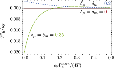
Figure 5: Nematic coupling constant $g$ in the presence intraband scattering in the hole band, characterized by the scattering rate $\Gamma_{\mathrm{h}}^{\mathrm{intra}}$. We chose $\delta_{\mu}=\delta_{m}=0.2$ (blue, dotted line) as an example of small ellipticity and detuning which guarantees $w<0$ and $g>0$, and $\delta_{\mu}=\delta_{m}=0.35$ (green, dashed line) as an example where disorder can tune $g$ and $w$ to be either positive or negative. The red lines represent the results at particle-hole symmetry, $\delta_{\mu}=\delta_{m}=0$.

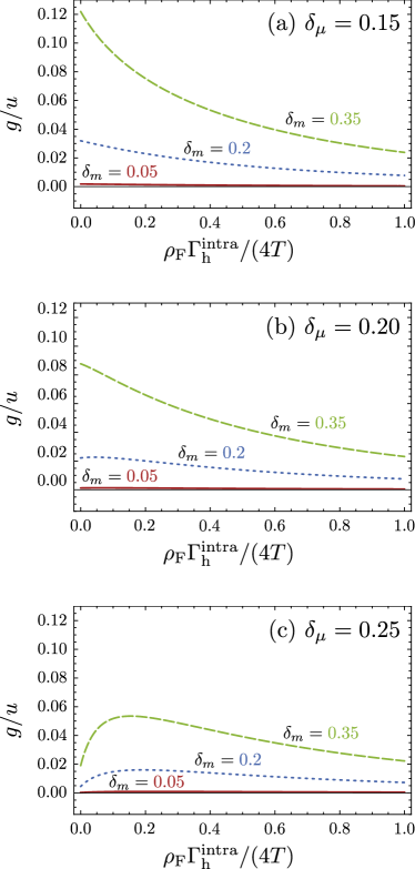
Figure 6: Dependence of the dimensionless nematic coupling constant $g/u$ on disorder. (a) Close to particle-hole symmetry, $g/u$ decreases monotonically with increasing scattering rate. (b) and (c) With increasing distance to particle-hole symmetry, an initial increase of the dimensionless nematic coupling constant is found for small scattering rates, but for stronger disorder, the ratio $g/u$ decreases again.

Even when the suppression of $g$ by disorder does not induce a sign-change, it has important consequences for the phase diagram. In particular, as shown in Ref. Fernandes et al., 2012a, the splitting $\Delta T=T_{\mathrm{s}}-T_{\mathrm{N}}$ between the nematic/structural and the magnetic transitions is controlled by the inverse dimensionless nematic coupling constant $u/g$ and the dimensionality $d$. In particular, for $2<d<3$, which mimics an anisotropic 3D system, the two transitions are simultaneous and first order for $\left(u/g\right)<\left(u/g\right)_{c_{1}}=1/\left(3-d\right)$. For $(u/g)_{c_{1}}<(u/g)<(u/g)_{c_{2}}$, the transitions are split and one of them remains first-order whereas the other transition is second-order. In this regime, an increase in $u/g$ results in an enhanced splitting $\Delta T$, whereas deep in the regime of two split second-order phase transitions, $\left(u/g\right)\gg\left(u/g\right)_{c_{2}}=\left(6-d\right)/\left(6-2d\right)$, increasing the ratio $u/g$ reduces the splitting $\Delta T$. To compute the dimensionless parameter $u/g$, we compute $u$ analogously to the case of $g$

$$u =\frac{T}{2}\sum_{n}\int\frac{\mathrm{d}\boldsymbol{\mathbf{k}}}{(2\pi)^{2}}\,G_{\mathrm{h}_{\Gamma},\boldsymbol{\mathbf{k}}}^{2}(\nu_{n})\left[G_{\mathrm{e}_{1},\boldsymbol{\mathbf{k}}}(\nu_{n})+G_{\mathrm{e}_{2},\boldsymbol{\mathbf{k}}}(\nu_{n})\right]^{2}+\Gamma_{\mathrm{h}}^{\mathrm{intra}}\frac{T}{2}\sum_{n}\left[\int\frac{\mathrm{d}\boldsymbol{\mathbf{k}}}{(2\pi)^{2}}\,G_{\mathrm{h}_{\Gamma},\boldsymbol{\mathbf{k}}}^{2}(\nu_{n})[G_{\mathrm{e}_{1},\boldsymbol{\mathbf{k}}}(\nu_{n})+G_{\mathrm{e}_{2},\boldsymbol{\mathbf{k}}}(\nu_{n})]\right]^{2}$$

$$=\mathcal{G}_{1}^{(1)}+\mathcal{G}_{2}^{(1)}+\mathcal{G}_{1}^{(2)}+\mathcal{G}_{2}^{(2)}=-\frac{\rho_{\mathrm{F}}}{8\pi^{2}T^{2}}\left[\operatorname{\psi_{2}}\Big{(}\frac{1}{2}+\frac{\rho_{\mathrm{F}}\Gamma_{\mathrm{h}}^{\mathrm{intra}}}{4T}\Big{)}+\frac{\rho_{\mathrm{F}}\Gamma_{\mathrm{h}}^{\mathrm{intra}}}{12T}\operatorname{\psi_{3}}\Big{(}\frac{1}{2}+\frac{\rho_{\mathrm{F}}\Gamma_{\mathrm{h}}^{\mathrm{intra}}}{4T}\Big{)}\right]$$

$$\qquad\qquad+\frac{\rho_{\mathrm{F}}}{768\pi^{4}T^{4}}\operatorname{\psi_{4}}\Big{(}\frac{1}{2}+\frac{\rho_{\mathrm{F}}\Gamma}{4T}\Big{)}\left[3\delta_{\mu}^{2}+\delta_{m}^{2}\right]+\frac{\rho_{\mathrm{F}}^{2}\Gamma_{\mathrm{h}}^{\mathrm{intra}}}{30720\pi^{4}T^{5}}\operatorname{\psi_{5}}\Big{(}\frac{1}{2}+\frac{\rho_{\mathrm{F}}\Gamma}{4T}\Big{)}\left[10\delta_{\mu}^{2}+3\delta_{m}^{2}\right]$$ (15)

in accordance with previous work. Hoyer et al. (2014) Near particle-hole symmetry, where $\delta_{\mu}/(2\pi T)$ and $\delta_{m}/(2\pi T)$ are sufficiently small, and the magnetic ground state is the stripe one, $g/u$ decreases monotonically with increasing scattering rate as shown in Fig. 6(a). Thus, if the system initially is near the regime of first-order simultaneous transitions, as it is the case in undoped BaFe₂As₂, the addition of disorder is expected to cause (or enhance) a splitting in the magnetic and structural transitions. This agrees with recent experiments in BaFe₂As₂, which observed enhanced splitting of the transitions upon electron irradiation.Takasada Shibauchi This result is also consistent with the theoretical finding of Ref. Liang et al., 2015 that disorder stabilizes the nematic phase. We note, however, that the dependence of the ratio $g/u$ on disorder is nonuniversal (see Fig. 6(b) and (c)). In particular, farther away from particle-hole symmetry, the dependence of $g/u$ on disorder is no longer monotonic: $g/u$ first increases with increasing scattering rate, and above a critical value starts decreasing again.

III.2 Effect of disorder on the planar coupling $w$

Having established that $g$ can become either positive or negative in both clean and dirty systems, we now analyze $w$. As discussed above and illustrated in Fig. 3(a), in the clean three-band model $w=0$ always. Following the analysis of the generic fourth-order diagram in Fig. 3 and Eq. (7), the only scattering processes that gives rise to a nonzero contribution to $w$ is the one coupling the electron pocket at $\boldsymbol{\mathbf{Q}}_{1}$ and the electron pocket at $\boldsymbol{\mathbf{Q}}_{2}$, characterized by the scattering rate $\Gamma_{\mathrm{e-e}}^{\mathrm{inter}}$. For the sake of clarity, we neglect all other interband scattering processes since they give subleading contributions to $w$, i.e. $w=0$ always as long as $\Gamma_{\mathrm{e-e}}^{\mathrm{inter}}=0$. Then, in the presence of the dominant scattering process, intraband scattering in the hole band and, additionally, interband scattering between the electron bands, we find

$$w =2\Gamma_{\mathrm{e-e}}^{\mathrm{inter}}T\sum_{n}\!\Big{[}\!\int\!\!\frac{\mathrm{d}\boldsymbol{\mathbf{k}}}{(2\pi)^{2}}\,G_{\mathrm{h}_{\Gamma},\boldsymbol{\mathbf{k}}}(\nu_{n})G_{\mathrm{e}_{1},\boldsymbol{\mathbf{k}}}(\nu_{n})G_{\mathrm{e}_{2},\boldsymbol{\mathbf{k}}}(\nu_{n})\Big{]}^{2}$$

$$=2\mathcal{W}=-\frac{\rho_{\mathrm{F}}^{2}\Gamma_{\mathrm{e-e}}^{\mathrm{inter}}}{96\pi^{2}T^{3}}\left[\operatorname{\psi_{3}}\Big{(}\frac{1}{2}+\frac{\rho_{\mathrm{F}}(\Gamma_{\mathrm{h}}^{\mathrm{intra}}+\Gamma_{\mathrm{e-e}}^{\mathrm{inter}})}{4T}\Big{)}\right.$$

$$\qquad\qquad\left.-\frac{10\delta_{\mu}^{2}+\delta_{m}^{2}}{320\pi^{2}T^{2}}\operatorname{\psi_{5}}\Big{(}\frac{1}{2}+\frac{\rho_{\mathrm{F}}(\Gamma_{\mathrm{h}}^{\mathrm{intra}}+\Gamma_{\mathrm{e-e}}^{\mathrm{inter}})}{4T}\Big{)}\right]~{},$$ (16)

where we assumed the density of states at the Fermi surface to be given by a constant $\rho_{\mathrm{F}}$ in all three bands, and we expanded to leading order in $\delta_{\mu}$ and $\delta_{m}$ to obtain the results. The respective diagram denoted by $\mathcal{W}$ is depicted in Fig. 4(c). Note that contributions with more than one scattering process between electron bands vanish upon momentum integration and thus the above result already includes contributions up to infinite order in $\Gamma_{\mathrm{e-e}}^{\mathrm{inter}}$.

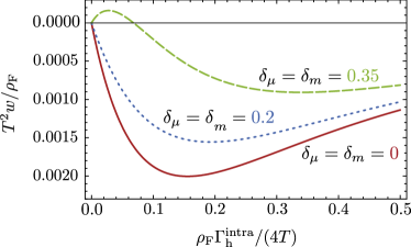
Figure 7: Planar coupling $w$ as a function of intraband scattering rate in the hole band, $\Gamma_{\mathrm{h}}^{\mathrm{intra}}$, where we set $\Gamma_{\mathrm{e-e}}^{\mathrm{inter}}=0.1\Gamma_{\mathrm{h}}^{\mathrm{intra}}$. We chose $\delta_{\mu}=\delta_{m}=0.2$ (blue, dotted line) as an example of small ellipticity and detuning which guarantees $w<0$ and $g>0$, and $\delta_{\mu}=\delta_{m}=0.35$ (green, dashed line) as an example where disorder can tune $w$ and $g$ to be either positive or negative. The red lines represent the results at particle-hole symmetry, $\delta_{\mu}=\delta_{m}=0$.

We show the coefficient $w$ as a function of the scattering rate for different values of detuning $\delta_{\mu}$ and ellipticity $\delta_{m}$ in Fig. 7. In the absence of impurity scattering, we recover $w=0$. At particle-hole symmetry, $\delta_{\mu}=\delta_{m}=0$, disorder leads to $w<0$, thus favoring the formation of a charge-spin density wave (see Fig. 1(a)) as long as $g<|w|$. In contrast, finite detuning and ellipticity yield a contribution of opposite sign and thus, depending on the scattering rate and the distance from particle-hole symmetry, $w$ can be either positive or negative, allowing for both proposed double-$\boldsymbol{\mathbf{Q}}$ states, CSDW and the SVC. This conclusion holds also in the presence of magnetic impurities. In this case, however, the global prefactor and the total scattering rate are altered as compared to the case of nonmagnetic impurities since for magnetic impurities, the evaluation of the trace $\operatorname{tr}[\sigma_{i}\sigma_{j}\sigma_{k}\sigma_{l}\sigma_{j}\sigma_{m}]$ allows for additional contributions including other interband scattering processes between the electron pockets $\mathrm{e}_{1}$ and $\mathrm{e}_{2}$.

IV Summary and Conclusions

Recent experiments revealed the existence of $C_{4}$-magnetic phases in hole-doped iron-based superconductors, further fueling the discussion about the nature of the magnetic ground state of the parent compounds. We considered a three-band model of iron-based superconductors complemented by an incipient fourth pocket at the $M$ point and investigated how the interplay of impurity scattering and disorder effects in a rigid-band approach affect the magnetic ground state.

The phase diagram is governed by the interplay of nematic and planar couplings, $g$ and $w$, respectively. If $g>\max(0,-w)$, stripe-magnetic order with either $\boldsymbol{\mathbf{M}}_{1}=0$ or $\boldsymbol{\mathbf{M}}_{2}=0$ is favored, as it has been observed in many compounds of the iron pnictide and iron chalcogenide families. If $g<\max(0,-w)$, a double-$\boldsymbol{\mathbf{Q}}$ state with $|\boldsymbol{\mathbf{M}}_{1}|=|\boldsymbol{\mathbf{M}}_{2}|$ minimizes the free energy, and the sign of $w$ determines whether $\boldsymbol{\mathbf{M}}_{1}\perp\boldsymbol{\mathbf{M}}_{2}$ (spin vortex crystal, for $w>0$) or $\boldsymbol{\mathbf{M}}_{1}=\pm\boldsymbol{\mathbf{M}}_{2}$ (charge-spin density wave, for $w<0$) is more favorable. So far, only the charge-spin density wave has been observed experimentally, J. M. Allred et al. ; Waßer et al. (2015); Mallett et al. (2015) in contrast to theoretical models. Chandra et al. (1990); Eremin and Chubukov (2010); Wang et al. (2015)

Although generic three-band low-energy models for the description of FeSC allow for $C_{4}$-magnetic ground states, they leave the spin vortex crystal (SVC) and the charge-spin density wave (CSDW) degenerate since $w=0$. Our analysis shows that the existence of an incipient pocket at $(\pi,\pi)$ lifts the degeneracy, however, it would favor the formation of a spin-vortex crystal ($w>0$) and thus cannot explain the experimental findings. The investigation of other extensions to the three-band model such as the consideration of additional interactions has lead to the same conclusion that the SVC state is favorable.

Our investigation of impurity scattering, in contrast, provides a natural explanation for the formation of a charge-spin density wave in doped FeSC. Since the three-band model under consideration yields $w=0$ in the absence of impurity scattering, we concentrated on the interband scattering process between the two electron bands that can render $w$ finite. In addition, we considered intraband scattering in all three bands. We find $w<0$ at particle-hole symmetry as well as for small ellipticity and detuning, suggesting that disorder can promote charge-spin density waves. However, sufficiently large ellipticity and detuning in combination with impurity scattering also allow for $w>0$, i. e., a spin vortex crystal.

Our findings are summarized in the phase diagrams depicted in Fig. 2 where we show the magnetic ground states that are favored in different regimes of detuning and ellipticity. Disorder favors the double-Q charge-spin density wave over the single-Q stripe-magnetic SDW at small ellipticity and detuning, and increasing scattering rate increases the parameter regime in which CSDW order is expected to occur.

We further investigated the effect of the dominant impurity scattering process in FeSC, intraband scattering in the hole band, on the nematic coupling $g$, which in the three-band model assumes a finite value as long as the electron bands exhibit finite ellipticity. In the absence of impurity scattering and for $\delta_{\mu}=0$, $g$ is positive, and increasing intraband scattering in the hole band reduces the nematic coupling constant, concordant with the experimental finding that electron irradiation enhances the splitting between structural and magnetic transition in the stripe-ordered phase.

Previously, controlled disorder has been proposed as a way to tune the properties of the superconducting state in the iron-based materials.Wang et al. (2013) Analogously, our findings provide a promising control knob to tune their magnetic ground state. In particular, addition of impurities via electron irradiation in hole-doped compounds near the composition where the single-Q to double-Q magnetic transition is observed could stabilize a $C_{4}$-magnetic phase as the leading instability of the system – currently, the $C_{4}$-magnetic phase has been mostly observed inside the $C_{2}$-magnetic phase boundary. Similarly, removal of impurities via annealing in samples that display the double-Q magnetic order could change the nature of the $C_{4}$ phase from charge-spin density wave to spin-vortex crystal.

References

- Paglione and Greene (2010) Johnpierre Paglione and Richard L. Greene, “High-temperature superconductivity in iron-based materials,” Nature Physics 6, 645–658 (2010).
- Andrey V. Chubukov and Peter J. Hirschfeld (2015) Andrey V. Chubukov and Peter J. Hirschfeld, “Fe-based superconductors: seven years later,” Physics Today 68, 46 (2015).
- Pratt et al. (2009) D. K. Pratt, W. Tian, A. Kreyssig, J. L. Zarestky, S. Nandi, N. Ni, S. L. Bud’ko, P. C. Canfield, A. I. Goldman, and R. J. McQueeney, “Coexistence of competing antiferromagnetic and superconducting phases in the underdoped Ba(Fe0.953Co0.047)2As2 compound using x-ray and neutron scattering techniques,” Phys. Rev. Lett. 103, 087001 (2009).
- Laplace et al. (2009) Y. Laplace, J. Bobroff, F. Rullier-Albenque, D. Colson, and A. Forget, “Atomic coexistence of superconductivity and incommensurate magnetic order in the pnictide Ba(Fe1-xCox)2As2,” Phys. Rev. B 80, 140501 (2009).
- Fang et al. (2008) Chen Fang, Hong Yao, Wei-Feng Tsai, JiangPing Hu, and Steven A. Kivelson, “Theory of electron nematic order in LaFeAsO,” Phys. Rev. B 77, 224509 (2008).
- Xu et al. (2008) Cenke Xu, Markus Müller, and Subir Sachdev, “Ising and spin orders in the iron-based superconductors,” Phys. Rev. B 78, 020501 (2008).
- R. M. Fernandes et al. (2014) R. M. Fernandes, A. V. Chubukov, and J. Schmalian, “What drives nematic order in iron-based superconductors?” Nat. Phys. 10, 97–104 (2014).
- Jesche et al. (2010) A. Jesche, C. Krellner, M. de Souza, M. Lang, and C. Geibel, “Coupling between the structural and magnetic transition in CeFeAsO,” Phys. Rev. B 81, 134525 (2010).
- (9) Takasada Shibauchi, private communication .
- Liang et al. (2015) Shuhua Liang, Christopher B. Bishop, Adriana Moreo, and Elbio Dagotto, “Isotropic in-plane quenched disorder and dilution induce a robust nematic state in electron-doped pnictides,” Phys. Rev. B 92, 104512 (2015).
- Kim et al. (2010) M. G. Kim, A. Kreyssig, A. Thaler, D. K. Pratt, W. Tian, J. L. Zarestky, M. A. Green, S. L. Bud’ko, P. C. Canfield, R. J. McQueeney, and A. I. Goldman, “Antiferromagnetic ordering in the absence of structural distortion in Ba,” Phys. Rev. B 82, 220503(R) (2010).
- Avci S. et al. (2014) Avci S., Chmaissem O., Allred J.M., Rosenkranz S., Eremin I., Chubukov A.V., Bugaris D.E., Chung D.Y., Kanatzidis M.G., Castellan J.-P, Schlueter J.A., Claus H., Khalyavin D.D., Manuel P., Daoud-Aladine A., and Osborn R., “Magnetically driven suppression of nematic order in an iron-based superconductor,” Nat Commun 5, 3845 (2014).
- Hassinger et al. (2012) E. Hassinger, G. Gredat, F. Valade, S. René de Cotret, A. Juneau-Fecteau, J.-Ph. Reid, H. Kim, M. A. Tanatar, R. Prozorov, B. Shen, H.-H. Wen, N. Doiron-Leyraud, and Louis Taillefer, “Pressure-induced Fermi-surface reconstruction in the iron-arsenide superconductor Ba1-xKxFe2As2: Evidence of a phase transition inside the antiferromagnetic phase,” Phys. Rev. B 86, 140502 (2012).
- Böhmer A. E. et al. (2015) Böhmer A. E., Hardy F., Wang L., Wolf T., Schweiss P., and Meingast C., “Superconductivity-induced re-entrance of the orthorhombic distortion in Ba1-xKxFe2As2,” Nat Commun 6, 7911 (2015).
- Allred et al. (2015) J. M. Allred, S. Avci, D. Y. Chung, H. Claus, D. D. Khalyavin, P. Manuel, K. M. Taddei, M. G. Kanatzidis, S. Rosenkranz, R. Osborn, and O. Chmaissem, “Tetragonal magnetic phase in Ba1-xKxFe2As2 from x-ray and neutron diffraction,” Phys. Rev. B 92, 094515 (2015).
- (16) J. M. Allred, K. M. Taddei, D. E. Bugaris, M. J. Krogstad, S. H. Lapidus, D. Y. Chung, H. Claus, M. G. Kanatzidis, D. E. Brown, J. Kang, R. M. Fernandes, I. Eremin, S. Rosenkranz, O. Chmaissem, and R. Osborn, “Double-Q spin-density wave in iron arsenide superconductors,” arXiv:1505.06175 .
- Wang et al. (2015) Xiaoyu Wang, Jian Kang, and Rafael M. Fernandes, “Magnetic order without tetragonal-symmetry-breaking in iron arsenides: Microscopic mechanism and spin-wave spectrum,” Phys. Rev. B 91, 024401 (2015).
- R. M. Fernandes et al. (2015) R. M. Fernandes, S. A. Kivelson, and E. Berg, “Is there a hidden chiral density-wave in the iron-based superconductors?” arXiv:1504.03656 (2015).
- Lorenzana et al. (2008) J. Lorenzana, G. Seibold, C. Ortix, and M. Grilli, “Competing orders in FeAs layers,” Phys. Rev. Lett. 101, 186402 (2008).
- Eremin and Chubukov (2010) I. Eremin and A. V. Chubukov, “Magnetic degeneracy and hidden metallicity of the spin-density-wave state in ferropnictides,” Phys. Rev. B 81, 024511 (2010).
- Kang and Tešanović (2011) Jian Kang and Zlatko Tešanović, “Theory of the valley-density wave and hidden order in iron pnictides,” Phys. Rev. B 83, 020505 (2011).
- Gianluca Giovannetti et al. (2011) Gianluca Giovannetti, Carmine Ortix, Martijn Marsman, Massimo Capone, Jeroen von den Brink, and José Lorenzana, “Proximity of iron pnictide superconductors to a quantum tricritical point,” Nature Communications 2, 398 (2011).
- Brydon et al. (2011) P. M. R. Brydon, Jacob Schmiedt, and Carsten Timm, “Microscopically derived Ginzburg-Landau theory for magnetic order in the iron pnictides,” Phys. Rev. B 84, 214510 (2011).
- Fernandes et al. (2012a) R. M. Fernandes, A. V. Chubukov, J. Knolle, I. Eremin, and J. Schmalian, “Preemptive nematic order, pseudogap, and orbital order in the iron pnictides,” Phys. Rev. B 85, 024534 (2012a).
- Cvetkovic and Vafek (2013) Vladimir Cvetkovic and Oskar Vafek, “Space group symmetry, spin-orbit coupling, and the low-energy effective hamiltonian for iron-based superconductors,” Phys. Rev. B 88, 134510 (2013).
- Kang et al. (2015) Jian Kang, Xiaoyu Wang, Andrey V. Chubukov, and Rafael M. Fernandes, “Interplay between tetragonal magnetic order, stripe magnetism, and superconductivity in iron-based materials,” Phys. Rev. B 91, 121104 (2015).
- Gastiasoro and Andersen (2015) Maria N. Gastiasoro and Brian M. Andersen, “Competing magnetic double- phases and superconductivity-induced reentrance of magnetic stripe order in iron pnictides,” Phys. Rev. B 92, 140506 (2015).
- Wang and Fernandes (2014) Xiaoyu Wang and Rafael M. Fernandes, “Impact of local-moment fluctuations on the magnetic degeneracy of iron arsenide superconductors,” Phys. Rev. B 89, 144502 (2014).
- Waßer et al. (2015) F. Waßer, A. Schneidewind, Y. Sidis, S. Wurmehl, S. Aswartham, B. Büchner, and M. Braden, “Spin reorientation in Ba0.65Na0.35Fe2As2 studied by single-crystal neutron diffraction,” Phys. Rev. B 91, 060505 (2015).
- Mallett et al. (2015) B. P. P. Mallett, Yu. G. Pashkevich, A. Gusev, Th. Wolf, and C. Bernhard, “Muon spin rotation study of the magnetic structure in the tetragonal antiferromagnetic state of weakly underdoped Ba1-xKxFe2As2,” EPL 111, 57001 (2015).
- Chandra et al. (1990) P. Chandra, P. Coleman, and A. I. Larkin, “Ising transition in frustrated Heisenberg models,” Phys. Rev. Lett. 64, 88–91 (1990).
- (32) Morten H. Christensen, Jian Kang, Brian M. Andersen, Ilya Eremin, and Rafael M. Fernandes, “Spin reorientation driven by the interplay between spin-orbit coupling and Hund’s rule coupling in iron pnictides,” arXiv:1508.01763 .
- Fernandes et al. (2012b) R. M. Fernandes, M. G. Vavilov, and A. V. Chubukov, “Enhancement of by disorder in underdoped iron pnictide superconductors,” Phys. Rev. B 85, 140512 (2012b).
- Wadati et al. (2010) H. Wadati, I. Elfimov, and G. A. Sawatzky, “Where are the extra electrons in transition-metal-substituted iron pnictides?” Phys. Rev. Lett. 105, 157004 (2010).
- Hoyer et al. (2015) M. Hoyer, M. S. Scheurer, S. V. Syzranov, and J. Schmalian, “Pair breaking due to orbital magnetism in iron-based superconductors,” Phys. Rev. B 91, 054501 (2015).
- Karkin et al. (2009) A. E. Karkin, J. Werner, G. Behr, and B. N. Goshchitskii, “Neutron-irradiation effects in polycrystalline LaFeAsO0.9F0.1 superconductors,” Phys. Rev. B 80, 174512 (2009).
- Li et al. (2011) Jun Li, Yanfeng Guo, Shoubao Zhang, Shan Yu, Yoshihiro Tsujimoto, Hiroshi Kontani, Kazunari Yamaura, and Eiji Takayama-Muromachi, “Linear decrease of critical temperature with increasing Zn substitution in the iron-based superconductor BaFe1.89-2xZn2xCo0.11As2,” Phys. Rev. B 84, 020513 (2011).
- Kirshenbaum et al. (2012) Kevin Kirshenbaum, S. R. Saha, S. Ziemak, T. Drye, and J. Paglione, “Universal pair-breaking in transition-metal-substituted iron-pnictide superconductors,” Phys. Rev. B 86, 140505 (2012).
- Rullier-Albenque et al. (2009) F. Rullier-Albenque, D. Colson, A. Forget, and H. Alloul, “Hall Effect and Resistivity Study of the Magnetic Transition, Carrier Content, and Fermi-Liquid Behavior in Ba(Fe1-xCox)2As2,” Phys. Rev. Lett. 103, 057001 (2009).
- Fang et al. (2009) Lei Fang, Huiqian Luo, Peng Cheng, Zhaosheng Wang, Ying Jia, Gang Mu, Bing Shen, I. I. Mazin, Lei Shan, Cong Ren, and Hai-Hu Wen, “Roles of multiband effects and electron-hole asymmetry in the superconductivity and normal-state properties of Ba(Fe1-xCox)2As2,” Phys. Rev. B 80, 140508 (2009).
- Allan et al. (2012) M. P. Allan, A. W. Rost, A. P. Mackenzie, Y. Xie, J. C. Davis, K. Kihou, C. H. Lee, A. Iyo, H. Eisaki, and T.-M. Chuang, “Anisotropic Energy Gaps of Iron-Based Superconductivity from Intraband Quasiparticle Interference in LiFeAs,” Science 336, 563–567 (2012).
- Berlijn et al. (2012) Tom Berlijn, Chia-Hui Lin, William Garber, and Wei Ku, “Do transition-metal substitutions dope carriers in iron-based superconductors?” Phys. Rev. Lett. 108, 207003 (2012).
- Alexander Herbig et al. (2015) Alexander Herbig, Rolf Heid, and Jörg Schmalian, “Charge doping versus impurity scattering in chemically substituted iron-pnictides,” arXiv:1510.06941 (2015).
- Fanfarillo et al. (2015) Laura Fanfarillo, Alberto Cortijo, and Belén Valenzuela, “Spin-orbital interplay and topology in the nematic phase of iron pnictides,” Phys. Rev. B 91, 214515 (2015).
- Hoyer et al. (2014) M. Hoyer, S. V. Syzranov, and J. Schmalian, “Effect of weak disorder on the phase competition in iron pnictides,” Phys. Rev. B 89, 214504 (2014).
- Wang et al. (2013) Y. Wang, A. Kreisel, P. J. Hirschfeld, and V. Mishra, “Using controlled disorder to distinguish and gap structure in Fe-based superconductors,” Phys. Rev. B 87, 094504 (2013).