Chaos-assisted formation of immiscible matter-wave solitons and self-stabilization in the binary discrete nonlinear Schrödinger equation

Abstract

Binary discrete nonlinear Schrödinger equation is used to describe dynamics of two-species Bose-Einstein condensate loaded into an optical lattice. Linear inter-species coupling leads to Rabi transitions between the species. In the regime of strong nonlinearity, a wavepacket corresponding to condensate separates into localized and ballistic fractions. Localized fraction is predominantly formed by immiscible solitons consisted of only one species. Initial states without spatial separation of occupied sites expose formation of immiscible solitons after a strongly chaotic transient. We calculate the finite-time Lyapunov exponent as a rate of wavepacket divergence in the Hilbert space. Using the Lyapunov analysis supplemented by Monte-Carlo sampling, it is shown that appearance of immiscible solitons after the chaotic transient corresponds to self-stabilization of the wavepacket. It is found that onset of chaos is accompanied by fast variations of kinetic and interaction energies. Crossover to self-stabilization is accompanied by reduction of condensate density due to emittance of ballistically propagating waves. It turns out that spatial separation of species should be a necessary condition for wavepacket stability in the presence of linear inter-species coupling.

1 Introduction

Discrete nonlinear Schrödinger equation (DNLSE) being coupled system of nonlinear ordinary differential equations occurs in variety of physical problems [1]. For example, DNLSE describes light propagation in periodic waveguide arrays. If the array consists of two distinct chains coupled to each other, then a light wavefield is governed by the binary DNLSE [2]. Recently such configuration was exploited for optical simulation of neutrino oscillations, and formation of neutrino solitons was predicted [3]. In quantum optics, DNLSE is utilized for studying Bose-Einstein condensate (BEC) loaded into an optical lattice. Binary DNLSE occurs if the condensate is a mixture of two different atomic species. The species may correspond to different atoms, for example, ¹³³Cs and ⁸⁷Rb [4]. Another possibility is the mixture of atoms of the same sort but belonging to different hyperfine states [5]. In the latter case the species can be transformed to each other by means of external electromagnetic field giving rise to resonant transitions between the hyperfine states.

One of the main properties of the DNLSE is the onset of discrete solitons and/or breathers when the nonlinearity is strong enough [6, 7, 8]. Under certain conditions, their formation can be studied within the variational approach that relies upon a priori assumptions about the wavepacket form in course of its evolution [9]. However, as it was found in a recent work [10], solitons in the binary DNLSE can arise spontaneously after a transient regime of highly irregular dynamics, when the variational approach doesn’t apply. A distinctive feature of such solitons is that they consist of only one species and well separated from each other. In the case of BEC mixtures loaded into optical lattices, onset of one-species (i.e., immiscible) solitons corresponds to the miscible-immiscible quantum phase transition [11, 12, 13] being a form of spontaneous symmetry breaking [14, 15].

In the present work, we examine the link between the spontaneous formation of matter-wave solitons and Lyapunov stability. Our attention is concentrated on the regime of strong nonlinearity that corresponds to more extensive interaction between atoms and anticipates more pronounced manifestation of chaos.

The paper is organized as follows. In the next section we describe the model under consideration. Section 3 represents some generic features of condensate chaotic dynamics and soliton formation. The Monte-Carlo method is utilized for studying various aspects of wavepacket dynamics in Section 4. Section 5 is devoted to discussion of the main results and outlines some prospects for further research.

2 Basic equations

Binary DNLSE is given by the set of coupled ODE

$$i\hbar\frac{da_{n}}{dt} =-\frac{J}{2}(a_{n-1}+a_{n+1})+g_{11}|a_{n}|^{2}a_{n}+g_{12}|b_{n}|^{2}a_{n}-\frac{\hbar\Omega}{2}b_{n},$$ (1)

$$i\hbar\frac{db_{n}}{dt} =-\frac{J}{2}(b_{n-1}+b_{n+1})+g_{22}|b_{n}|^{2}b_{n}+g_{21}|a_{n}|^{2}b_{n}-\frac{\hbar\Omega}{2}a_{n}.$$

Our interest is mainly motivated by the problem of BEC dynamics in optical lattices. In this way, Eqs. (1) describe motion of two-species BEC mixture, where the species correspond to different hyperfine states. Quantities $a_{n}$ and $b_{n}$ are complex-valued amplitudes of BEC wave function at the lattice site $n$. $J$ is a hopping rate quantifying tunneling between neighbouring sites. $\Omega$ is a Rabi frequency being the rate of inter-species transitions between the hyperfine states under the action of the external rf radiation. Nonlinearity coefficients $g_{ij}$ are determined by $s$-wave scattering lengths and quantify strength of interaction between atoms. As in Ref. [10], we assume that the interaction between atoms belonging to different hyperfine states is weak and can be neglected, $g_{12}=g_{21}=0$. Indeed, both intra-species and inter-species scattering lengths can be readily tuned in experiments by means of the Feshbach resonance [16, 17], that is, one has some freedom in choosing their values. Also, it should be noted that intra-species dynamics rather depends on the difference of nonlinearity parameters

$$\Delta g=g_{11}+g_{22}-g_{12}-g_{21},$$ (2)

than on their absolute calues [18, 12], therefore one can regard the case of $g_{12}=g_{21}=0$ ($g_{11,22}\neq 0$) as the limiting regime when intra-species interaction dominates. As both species correspond to same sort of atoms, one can set $g_{11}=g_{22}\equiv g$. Thus, we arrive to a simplified form of (1)

$$i\hbar\frac{da_{n}}{dt} =-\frac{J}{2}(a_{n-1}+a_{n+1})+g|a_{n}|^{2}a_{n}-\frac{\hbar\Omega}{2}b_{n},$$ (3)

$$i\hbar\frac{db_{n}}{dt} =-\frac{J}{2}(b_{n-1}+b_{n+1})+g|b_{n}|^{2}b_{n}-\frac{\hbar\Omega}{2}a_{n},$$

Equations (3) can be also considered as the semiclassical limit of the corresponding two-species Bose-Hubbard model [13]. Hereafter we shall use the normalization condition

$$\sum\limits_{n=-N}^{N}\rho_{n}=1,\quad\rho_{n}=|a_{n}|^{2}+|b_{n}|^{2},$$ (4)

where $\rho_{n}$ is population of the site $n$, $2N+1$ is total number of sites. Amplitudes $a_{n}$ and $b_{n}$ can be represented as

$$a_{n}=\sqrt{A_{n}}e^{i\alpha_{n}},\quad b_{n}=\sqrt{B_{n}}e^{i\beta_{n}},\quad A_{n},B_{n},\alpha_{n},\beta_{n}\in\Re.$$ (5)

Substituting (5) into (1), we can rewrite (1) in the Hamiltonian form

$$\frac{dA_{n}}{dt} =-\frac{\partial H}{\partial\alpha_{n}},\quad\frac{d\alpha_{n}}{dt}=\frac{\partial H}{\partial A_{n}},$$ (6)

$$\frac{dB_{n}}{dt} =-\frac{\partial H}{\partial\beta_{n}},\quad\frac{d\beta_{n}}{dt}=\frac{\partial H}{\partial B_{n}}.$$

The corresponding Hamiltonian is given by the sum

$$H=H_{\text{kin}}+H_{\text{Rabi}}+H_{\text{int}},$$ (7)

where

$$H_{\text{kin}}=-J\sum\limits_{n=-N}^{N-1}[\sqrt{A_{n}A_{n+1}}\cos(\alpha_{n}-\alpha_{n+1})+\sqrt{B_{n}B_{n+1}}\cos(\beta_{n}-\beta_{n+1})]$$ (8)

is the kinetic energy,

$$H_{\text{Rabi}}=-\Omega\sum\limits_{n=-N}^{N}\sqrt{A_{n}B_{n}}\cos(\alpha_{n}-\beta_{n})$$ (9)

is the energy of inter-species coupling, or Rabi energy,

$$H_{\text{int}}=\frac{g}{2}\sum\limits_{n=-N}^{N}(A_{n}^{2}+B_{n}^{2})$$ (10)

is the energy of interaction between atoms belonging to the same species. Formally, the Hamiltonian described by (7)–(10) looks as Hamiltonian of a binary chain of classical particles with nearest-neighbour coupling that depends on $A_{n}$ and $B_{n}$ playing the role of “particle velocities”. Continuing this analogy, the term $H_{\text{int}}$ enters into the Hamiltonian as the “particle kinetic energy”, and $g$ is the inverse “mass”. One can easily see that in the limit $J,\Omega\to 0$ the equations (6) become integrable. This case corresponds to formation of one-site standing solitons, also known as compactons [19, 20, 21]. Presence of weak inter-cite couplings should not drastically destroy the integrability. One may expect that weak couplings should lead to the onset of exponential soliton tales. Thus, we can anticipate that formation of stable solitonic solutions should require interaction energy to be large compared to the kinetic and Rabi energies. This suggest that such solitons should be well spatially separated (in order to reduce the kinetic energy) and consist of only one species (to reduce the Rabi energy). Results of [10] indicate that solitons of this kind can arise spontaneously, provided wavepacket spreading is weak.

It is informative to consider the case of $J=0$ corresponding to a very deep lattice where neighbouring sites are decoupled. In this case Eqs. (6) can be transformed to the following form:

$$\frac{dz_{n}}{dt}=-\Omega\sqrt{1-z_{n}^{2}}\sin\chi_{n},\quad\frac{d\chi_{n}}{dt}=g\rho_{n}z_{n}+\frac{\Omega z_{n}}{\sqrt{1-z^{2}}}\cos\chi_{n},$$ (11)

where

$$z_{n}=\frac{A_{n}-B_{n}}{\rho_{n}},\quad\chi_{n}=\alpha_{n}-\beta_{n}.$$ (12)

Equations (11) originate from the Hamiltonian

$$\tilde{H}_{n}(z_{n},\,\chi_{n})=\frac{g\rho_{n}z_{n}^{2}}{2}-\Omega\sqrt{1-z_{n}^{2}}\cos\chi_{n}.$$ (13)

Qualitative behavior described by the Hamiltonian (13) crucially depends on the parameter

$$\Lambda_{n}=\frac{g\rho_{n}}{\Omega}.$$ (14)

If $\Lambda_{n}<1$, any trajectory of (11) is rotation in phase space around one of the center fixed points located at $z_{n}=0$, $\chi_{n}=k\pi$, $k=0,1$ [22]. It corresponds to oscillations of the population imbalance $z_{n}$ with zero mean. If $\Lambda_{n}>1$, the fixed point located at $z_{n}=0$, $\chi_{n}=\pi$ undergoes the pitchfork bifurcation and transforms into three fixed points, one saddle and two centers. The newborn center fixed points are located at $z_{n}=\pm\sqrt{1-\Lambda_{n}^{-2}}$, $\chi_{n}=\pi$. Each of them is surrounded by a domain of population imbalance oscillations with non-zero mean, that is, one species dominates over another. This regime can be referred to as the internal self-trapping. Further growth of the interaction strength $g$ moves the center fixed points towards the limiting values of population imbalance, $z_{n}=\pm 1$, and phase space area corresponding to the internal self-trapping increases.

3 Wavepacket dynamics for various initial conditions: main features

Figure 1: Participation ratio vs time for various forms of initial conditions.

In the present work we are aimed in studying formation of immiscible (i.e., one-species) solitons. Therefore we consider the regime of relatively strong nonlinearity $E_{\text{int}}/J\gg 1$, where $E_{\text{int}}=H_{\text{int}}(t=0)$. We use the following initial condition:

$$a_{n}(t=0)=A(p)\exp\left[-\frac{n^{2}}{4\sigma^{2}}\right]\cos{\pi pn},\quad b_{n}=0,$$ (15)

where $-N\leq n\leq N$, the factor $A$ is determined by the normalization condition (4). Parameter $\sigma$ characterizing wavepacket width is taken of 10. According to results of [10, 9], spatial dynamics of condensate depends on $E_{\text{int}}$ and the parameter $p$ describing spatial modulation. We consider three values of $p$: $p=0$ corresponding to the in-phase state, $p=1$ corresponding to the state with checkboard sequence of phases at lattice sites, and $p=0.5$ corresponding to the checkboard sequence, where all occupied sites are separated from each other by unoccupied ones.

Throughout this paper we use the following values of parameters: $J=2$, $\Omega=1$, $E_{\text{int}}=5$. It corresponds to the regime of strong nonlinearity anticipating extensive creation of localized states due to self-trapping. As values of the tunneling rate $J$ and Rabi frequency $\Omega$ are of the same order, one should expect strong interplay between spatial and internal dynamics. In numerical simulation, we used lattices with $N$ ranging from 4000 to 10000. A particular value for each calculation is chosen in order to avoid the influence of boundaries, therefore, it depends on a rate of spatial wavepacket expansion.

To quantify self-trapping, it is reasonable to consider participation ratio

$$\Gamma=\frac{1}{\sum\limits_{n}\rho_{n}^{2}}$$ (16)

being approximate number of occupied lattice sites. Figure 1 showing the time dependence of participation ratio confirms the significance of spatial modulation. Notably, self-trapping observed in the case of checkboard sequences $p=0.5$ and $p=1$ is much stronger than in the case of the in-phase state $p=0$.

Figure 2: Total population imbalance vs time for various forms of initial conditions.

Figure 3: Squared modulo of wavefunctions corresponding to the first (solid) and second (dotted) species at $t=500\pi$. (a) $p=0$, (b) $p=0.5$, (c) $p=1$.

Figure 4: Population imbalance (panels (a) and (b)) and population (panels (c) and (d)) at the lattice sites with $n=0$ ((a) and (c)) and $n=5$ ((b) and (d)).

As it was shown in [10], spatial self-trapping is accompanied by internal self-trapping, i.e., Rabi inter-species oscillations are suppressed and each soliton is predominantly formed by one species. We can call such solitons as immiscible solitons. As long as condensate fractions corresponding to the first and second species generally differ, total population imbalance

$$Z=\sum\limits_{n}\rho_{n}z_{n}=\sum\limits_{n}|a_{n}|^{2}-\sum\limits_{n}|b_{n}|^{2}.$$ (17)

can significantly deviate from zero. Time dependence of the total population imbalance is shown in Fig. 2. It is highly irregular indicating incoherence of Rabi oscillations running at different lattice sites. The first species notably dominates in the regime of the strongest self-trapping, corresponding to $p=0.5$. In contrast, the curves corresponding to $p=0$ and $p=1$ imply the presence of immiscible solitons corresponding to both species in comparable amounts. These suppositions are well confirmed by Fig. 3 illustrating wave states at $t=500\pi$. Each of the panels (a)–(c) represents series of localized immiscible states. In the case of $p=0.5$, all such states correspond to the first species, while the whole pattern looks like slightly distorted initial condition. In contrast, both species are present in the cases of $p=0$ and $p=1$, and there is no apparent similarity between the wavepacket patterns and the corresponding initial conditions. Absence of the similarity suggests that the patterns depicted in Fig. 3(a) and (c) should result from complicated evolution.

Metamorphoses happening to wavepackets are revealed in time dependences of population imbalance $z_{n}$ and population $\rho_{n}$ on individual lattice sites where solitons are pinned. Let’s consider the case of $p=0$ and the states localized at $n=0$ and $n=5$. The corresponding results are presented in Figure 4. On the initial stage, population imbalance experiences several bursts of stochastic oscillations until becomes localized near the limiting values: of -1 (for $n=0$) or 1 (for $n=5$). Comparing the time dependences of $z_{n}$ and $\rho_{n}$, one can see that stabilization of $z_{n}$ coincides with stabilization of $\rho_{n}$. It implies that the stabilization happens when matter flux through a site ceases. To achieve it, this site should have much larger population than on neighbouring sites, as this provides the spatial self-trapping [23]. It means that solitons are nucleated on specific density fluctuations. There is close analogy to emergence of solitons on impurities under conditions of spatiotemporal chaos [24].

According to Fig. 3, the state at $n=0$ consists of both species. Presence of the second species reveals itself in sporadic variations of $z_{0}$ and $\rho_{0}$ which are absent in the case of $n=5$. So, it turns out that admixture of another species acts as a destabilizing factor for dynamics, that is, well-isolated immiscible states should be the most stable configuration.

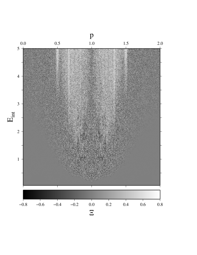
Figure 5: The order parameter being the population imbalance averaged over time interval $[900\pi:1000\pi]$ as function of parameters $E_{\text{int}}$ and $p$ characterizing the initial condition.

To describe the resulting solitonic patterns, we need a properly defined order parameter. Total population imbalance looks as a good candidate as it becomes non-zero as solitons appear, except for the case when solitons of different species give equal contributions and therefore compensate each other. In fact, the latter phenomenon can be readily considered as a rare event and therefore neglected. To eliminate contribution of non-solitonic states, we can average population imbalance over sufficiently long time interval. This interval must correspond to large enough times when all transient regimes are completed, and a wave field achieves some equillibrium state. Thus, we arrive to the following definition:

$$\Xi=\frac{1}{\Delta}\int\limits_{t^{\prime}-\Delta}^{t^{\prime}}Z(t)\,dt,$$ (18)

where $t^{\prime}=1000\pi$, $\Delta=100\pi$. Figure 5 demonstrates phase diagram of condensate in coordinates $p$ and $E_{\text{int}}$. Fine-grained structure of the diagram indicates high sensitivity of the order parameter to small changes in initial conditions, that is typical for chaos. Nevertheless, one can see vertical stripes with the prevailence of white, in particular, at $p=\pm 0.5$. These regions correspond to initial conditions which are more favorable for the solitons of the first species. Uniform region below the fine-grained pattern corresponds to dynamics without self-trapping, when population imbalance oscillates with zero mean.

4 Monte-Carlo sampling

4.1 Perturbation of initial conditions

Figure 6: Ensemble-averaged participation ratio (a) and its standard deviation (b) vs time.

Extreme sensitivity of wavepacket dynamics to small changes of initial conditions burdens analysis of physical condensate properties. Therefore, it is reasonable to use some statistical averaging in order to smooth that sensitivity out. Following this aim, we impose random perturbation on an initial state

$$\mathbf{a}(t=0) =\mathbf{a^{(0)}}(t=0)+\mathbf{\nu},$$ (19)

$$\mathbf{b}(t=0) =\mathbf{b^{(0)}}(t=0)+\mathbf{\xi},$$

where $\mathbf{a^{(0)}}(t=0)$ and $\mathbf{b^{(0)}}(t=0)$ are given by (15). Then we carry out the Monte-Carlo sampling over $\nu$ and $\xi$ realizations. Components of vectors $\mathbb{\nu}$ and $\mathbb{\xi}$ are Gaussian random variables whose moments obey the following formulae:

$$\left<\nu_{k}^{*}\xi_{k}\right>=0,\quad\left<\nu_{k}^{*}\nu_{l}\right>=\left<\xi_{k}^{*}\xi_{l}\right>=\delta_{kl}\frac{\varepsilon}{\sigma\sqrt{2\pi}}\exp\left[-\frac{k^{2}}{2\sigma^{2}}\right],$$ (20)

where $\delta_{kl}$ is the Kronecker symbol, and $\sigma$ takes on the same value as for original initial conditions. Taking into account the normalization condition (4), we set $\varepsilon=0.01$ providing weakness of the perturbation (19).

Figure 7: Ensemble-averaged wavepacket width defined by formula (21) as function of time.

Figure 8: Ensemble-averaged total population imbalance (a) and its standard deviation (b) vs time.

4.2 Spatial vs internal dynamics

Now let’s consider ensemble-averaged picture of spatial and internal dynamics. Ensemble-averaged participation ratio $\left<\Gamma\right>$ being a good indicator of the spatial self-trapping evolves in a very similar way as for non-distorted initial conditions (15). For all values of $p$, $\left<\Gamma\right>$ achieves a plateou and becomes almost constant, implying onset of self-trapping (see Fig. 6(a)). In the case of the in-phase state $p=0$, the plateou corresponds to significantly larger values of $\left<\Gamma\right>$ reflecting weaker self-trapping. Comparing Figs. 1 and 6(a), one can conclude that ensemble averaging smoothes out the small-scale fluctuations of participation ratio that are present in Fig. 1. Time dependence of $\sigma_{\Gamma}$, being standard deviation of $\Gamma$, deserves an intent look. In the case of $p=0.5$ it is almost constant, and the ratio $\sigma_{\Gamma}/\left<\Gamma\right>\simeq 0.02$ is very low revealing stable tendency to self-trapping. In contrast, $\sigma_{\Gamma}$ for $p=0$ and $p=1$ varies non-monotonically with time. Its local maximum precedes stopping of wavepacket expansion and onset of the self-trapping. After the self-trapping is happened, the standard deviation of $\Gamma$ becomes nearly constant, and ratio $\sigma_{\Gamma}/\left<\Gamma\right>$ is approximately three times larger than in the case of $p=0.5$. It indicates significantly higher diversity of solitonic configurations emerged.

Spatial expansion of a wavepacket can be described by the quantity

$$\sigma_{x}=\frac{1}{\sqrt{M}}\sqrt{\sum_{k}\Delta_{m}^{2}},\quad\Delta_{m}=\sum_{n}n^{2}\rho_{n}^{(m)}-\left(\sum_{n}n\rho_{n}^{(m)}\right)^{2},$$ (21)

where index $m$ numbers realizations of perturbations $\mathbf{\nu}$ and $\mathbf{\xi}$, $M$ is total number of realizations. Figure 7 shows that wavepackets are spreading ballistically despite of the spatial self-trapping and onset of solitons. It means coexistence of ballistic and localized parts of the condensate. Comparing the data corresponding to different $p$, we see that the most fast spreading is observed for the in-phase state.

Time dependence of the ensemble-averaged total population imbalance $\left<Z\right>$ has remarkable differences with that for non-distorted initial conditions. After rapid decreasing in the beginning, all the curves achieve a plateou whose position depends on initial state (see Fig. 8(a)). In the case of $p=0.5$ the plateou corresponds to $\left<Z\right>=0.74$ reflecting dominance of the first species. On the other hand, both species have the same statistical weights in the case of the in-phase state $p=0$. Dynamics of the state $p=1$ corresponds to an intermediate regime, when dominance of the first species is not so pronounced as in the case of $p=0.5$. Also, the case of $p=1$ demonstrates the largest values of standard deviation $\sigma_{Z}$ indicating the highest sensitivity of Rabi oscillations to small variations of initial conditions.

4.3 Lyapunov analysis

As it was shown in the preceding section, dynamics of binary BEC in an optical lattice in the regime of strong nonlinearity can exhibit highly irregular behavior. Extreme sensitivity to small distortions of a wavepacket infers dynamical chaos. As Eqs. (3) are nonlinear ODE, onset of chaos is not surprising [25, 26, 27]. As it was shown in [28], onset of dynamical chaos in BEC dynamics is closely related to the process of condensate depletion due to partial thermalization.

Chaos strength can be quantified by means of the maximal Lyapunov exponent. To determine it, we can use a concept being the discretized version of the definition used in [29]. In that work one considers distance between two wave states in the Hilbert space

$$D(t)=\frac{1}{2}\left<\Psi^{\prime}-\Psi|\Psi^{\prime}-\Psi\right>,$$ (22)

where $\Psi$ and $\Psi^{\prime}$ are solutions of the nonlinear Schrödinger equation with infinitesimal difference in initial conditions. Then the Lyapunov exponent can be determined as

$$\lambda=\lim\limits_{t\to\infty}\,\lim\limits_{D(0)\to 0}\frac{1}{2t}\ln\frac{D(t)}{D(0)}.$$ (23)

In analogy with [29], we can define the Lyapunov exponent for the binary DNLSE as

$$\lambda=\lim\limits_{t\to\infty}\,\lim\limits_{d(0)\to 0}\frac{1}{2t}\ln\frac{d(t)}{d(0)},$$ (24)

where

$$d(t)=\frac{1}{2}\sum\limits_{n}(\delta a_{n}^{*}\delta a_{n}+\delta b_{n}^{*}\delta b_{n}),$$ (25)

$$\delta a_{n}=\tilde{a}_{n}-a_{n},\quad\delta b_{n}=\tilde{b}_{n}-b_{n},$$ (26)

and the tilde denotes a solution with slightly perturbed initial conditions.

Despite of the importance of $\lambda$ as a chaos descriptor, it corresponds to the infinite-time limit and therefore doesn’t give physically relevant information about intermittency in course of evolution [30]. Therefore, it is reasonable to consider finite-time Lyapunov exponent (FTLE)

$$\lambda_{\Delta t}(\bar{t})=\frac{1}{2\Delta t}\lim\limits_{d(t_{0})\to 0}\ln\frac{d(t_{0}+\Delta t)}{d(t_{0})},\quad\bar{t}=t_{0}+\frac{\Delta t}{2}.$$ (27)

Figure 9: Mean finite-time Lyapunov exponent with $\Delta t=10\pi$ (a) and its rms value (b) vs time.

Figure 9(a) demonstrates time dependence of the mean FTLE. The curves corresponding to $p=0$ and $p=1$ reveal a crossover from chaotic to regular dynamics with increasing time. Standard deviation of the FTLE varies non-monotonically with time, as is shown in Fig. 9(b). Its maximum approximately corresponds to the time moment when nearly half of realizations have come into the regular regime. Notably, the crossover happens almost simultaneously for $p=0$ and $p=1$. As opposed to this, there is no apparent crossover in the case of $p=0.5$, and the mean FTLE, as well as its standard deviation, varies slowly with time. Values of the mean FTLE correspond to relatively weak chaos as compared to the initial stages in the cases of $p=0$ and $p=1$. Such behavior implies that the wavepacket with $p=0.5$ is close to some long-living state and therefore doesn’t experience any drastic changes of dynamics. On the other hand, this case doesn’t exhibit the self-stabilization as in the cases of $p=0$ and $p=1$. It means the presence of weak but persistent instability, that is, the initial state with $p=0.5$ should be rather regarded as metastable one.

4.4 Energy analysis

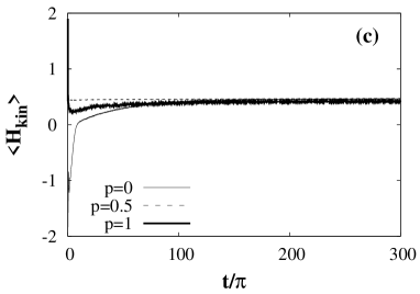
Figure 10: Ensemble-averaged interaction (a-b), kinetic (c-d) and Rabi (e-f) energies vs time for various initial conditions. Figures in the right column represent enlarged view of the beginning time intervals.

Energy conversion between components of the Hamiltonian (7) allows one to recover some specific features of wavepacket dynamics during the formation of immiscible solitons. Temporal variations of the interaction, kinetic and Rabi energies are presented in Fig. 10. One can see that exchange between the interaction and kinetic energies dominates, while variations of the Rabi energy are much lower in magnitude.

Firstly, let’s consider in detail the interaction energy (10). Owing to its definition, the interaction energy can serve a measure of wavepacket concentration and soliton formation. Quite surprisingly, the highest values of the interaction energy are observed in the case of $p=1$, not in the case of $p=0.5$ where soliton formation is the most pronounced. Another noticeable feature is extremely fast growth and decreasing of the interaction energy at the very beginning for $p=1$ and $p=0$, respectively. Comparison of Figs. 10(a) and (b) links the drastic variation of the interaction energy with the opposite variation (decreasing or increasing) of the kinetic energy. Intuitively, one can suggest that abrupt energy conversion should be a signature of strong instability and chaos ignition. So, it turns out that initial conditions with $p=0$ and $p=1$ are energetically unstable, in contrast to the case of $p=0.5$.

Another remarkable feature of the kinetic energy variations, presented in Fig. 10(b), is that the curves corresponding to different $p$ converge. It is reasonable to suggest that the main contribution into the kinetic energy is given from the ballistic fraction of condensate. This ballistic fraction corresponds to small-amplitude wavepackets emitted from the region occupied by solitons, i.e., the wavepacket origin. However, one should keep in mind that volume of the ballistic fraction strongly depends on $p$. For instance, it is much smaller in the case of $p=0.5$ than for other initial conditions. This phenomenon can be explained by the difference in total energy determined by the sum (7). Despite the absolute values of the kinetic energy are close to each other, their fractions in the total energy are different. So, relative contribution of the kinetic term into the total energy is the largest for $p=0$ and smallest for $p=0.5$.

Rabi energy (9) can be regarded as a measure of inter-species miscibility. Its time dependence is illustrated in Fig. 10(c). It is noticeable that the fast ignition of chaos for $p=0$ and $p=1$ in the beginning is accompanied by abrupt fast variations of the Rabi energy. Firstly, the Rabi energy fastly grows due to generation of the second species, and then there happens rapid spatial demixing of species. In the case of $p=0$ the species become almost completely demixed, that is, the ensemble-averaged Rabi energy is nearly zero. The demixing stage lasts several Rabi cycles. After that the Rabi energy starts increasing again, indicating creation of miscible states in the ballistic fraction. However, smallness of the Rabi energy variations infers smallness of population of miscible states. The main contribution into the miscible fraction is given from emitted ballistic wavepackets. Indeed, they have significantly lower density than localized states and, therefore, don’t experience the internal self-trapping.

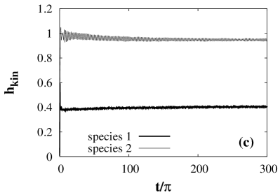
Figure 11: One-species kinetic (a, c, e) and interaction (b, d, f) energy densities as functions of time for initial states with $p=0$ (a, b), $p=0.5$ (c, d), $p=1$ (e, f).

It is informative to study how the kinetic and interaction energies are distributed over species. It can be done by means of the quantities

$$h_{\text{kin}}^{a,b}=\frac{\left<H_{\text{kin}}^{a,b}\right>}{\left<\rho_{a,b}\right>},\quad h_{\text{int}}^{a,b}=\frac{\left<H_{\text{int}}^{a,b}\right>}{\left<\rho_{a,b}\right>},$$ (28)

where

$$H_{\text{kin}}^{a} =-J\sum\limits_{n=-N}^{N-1}\sqrt{A_{n}A_{n+1}}\cos(\alpha_{n}-\alpha_{n+1}),$$ (29)

$$H_{\text{kin}}^{b} =-J\sum\limits_{n=-N}^{N-1}\sqrt{B_{n}B_{n+1}}\cos(\beta_{n}-\beta_{n+1}),$$

$$H_{\text{int}}^{a}=\frac{g}{2}\sum\limits_{n=-N}^{N}A_{n}^{2},\quad H_{\text{int}}^{b}=\frac{g}{2}\sum\limits_{n=-N}^{N}B_{n}^{2},$$ (30)

$$\rho_{a}\equiv\sum_{n}|a_{n}|^{2},\quad\rho_{b}\equiv\sum_{n}|b_{n}|^{2},$$ (31)

and angular brackets denote ensemble averaging. By definition, $h_{\text{kin}}^{a,b}$ and $h_{\text{int}}^{a,b}$ can be thought of as one-species densities of the kinetic and interaction energies, respectively. According to the data shown in Figure 11, only in the case of the in-phase state $p=0$ the energy densities are equally distributed among the species. In the cases of the checkboard states $p=0.5$ and $p=1$, the first species predominantly concentrates the interaction energy, while the second one has the larger kinetic energy. So, we can conditionally refer to them as “heavy” and “light” species, correspondingly. The heavy species is more apt to soliton formation, while the light species is more responsible for wavepacket spreading. Rabi inter-species coupling tends to remove distinction between the light and heavy species, at least, on statistical average, as in the case of $p=0$.

4.5 Spatial separation of species

Figure 12: Ensemble-averaged distance between species centers of mass vs time.

It should be noted that the initial states (15) for $p=0$, 0.5 and 1 are spatially symmetric. In the absence of random perturbations $\nu$ and $\xi$, this symmetry is preserved in course of evolution, even in the regime of dynamical chaos. It leads to the absence of center-of-mass motion. Inclusion of random perturbations (19) violate the spatial symmetry and there appears a possibility for mutual displacement of species, especially under the miscible/immiscible crossover. Let’s denote distance between species centers of mass as

$$\Delta n=\left<\left|n_{\text{a}}-n_{\text{b}}\right|\right>,$$ (32)

where

$$n_{\text{a}}=\frac{\sum_{n}n|a_{n}|^{2}}{\sum_{n}|a_{n}|^{2}},\quad n_{\text{b}}=\frac{\sum_{n}n|b_{n}|^{2}}{\sum_{n}|b_{n}|^{2}}.$$ (33)

Figure 12 shows that inter-species distance increases, on average, linearly with time, implying motion with constant velocity. The velocity depends on the parameter $p$: it is the largest in the case of $p=0.5$, while $p=0$ corresponds to the smallest velocity. Comparison of this dependence to the data presented in Fig. 8 indicates connection of the species separation to dynamics of Rabi inter-level oscillations. Indeed, it is reasonable to suggest that inter-species transformation has to reduce mean inter-species distance. So, the fastest separation is observed in the case of $p=0.5$, when Rabi oscillations are suppressed by the internal self-trapping.

5 Results and discussion

The present work is devoted to study of the binary discrete nonlinear Schrödinger equation (DNLSE) describing dynamics of two-species Bose-Einstein condensate loaded into an optical lattice. Different species are coupled to each other by external rf radiation causing inter-species transitions. Attention is concentrated on soliton formation and the miscible/immiscible crossover in the regime of strong nonlinearity, corresponding to high condensate density and/or strong inter-atomic coupling. We consider the case of comparable rates of tunneling and inter-species transitions, that is, these processes are competing with each other. It is found that condensate dynamics qualitatively depends on configuration of the initial state. The state being a sequence of occupied and unoccupied sites ($p=0.5$) exposes relatively stable dynamics with strong impact of self-trapping in both spatial and internal degrees of freedom. In contrast, initial states without unoccupied holes inside expose strong dynamical chaos revealing itself in highly irregular behavior of spatial structure and internal state. Onset of chaos is accompanied by drastic jump-like variations of the kinetic and interaction energies. Such jumps suggest that the corresponding initial conditions are far from bound states. So, one can conclude that stable solitonic configuration is possible only under spatial separation of solitons, like in the case of $p=0.5$.

Strength of chaos can be quantified by analysing evolution of distance in the Hilbert space between two initially close states. It allows one to define the corresponding Lyapunov exponent, as well as its finite-time counterpart. Lyapunov analysis shows that, after some beginning time interval, chaos ceases and dynamics acquires stability. Stabilization is accompanied by division of condensate onto localized and delocalized fractions. Localized fraction represents some kind of a equillibrium state being close to one of bound states. It consists of immiscible and spatially separated solitons. However, neither the positions of solitons nor the species they are formed by are predictable. Analysis by means of Monte-Carlo sampling shows that statistical properties of this equillibrium state also depend on a form of an initial state. In particular, the initial state with the checkboard phase configuration ($p=1$) leads to equillibrium states with higher density and, therefore, shows stronger tendency to spatial and internal self-trapping. In contrast, the in-phase initial state ($p=0$) exposes stronger impact of Rabi inter-species transitions that is reflected in zero ensemble-averaged population imbalance.

Phenomenon of the chaos-assisted soliton formation in Bose-Einstein condensates can be thought of as some manifestation of self-organization. Here one should remind that self-organization basically occurs in dissipative dynamical systems. Despite the discrete nonlinear Schrödinger equation has a Hamiltonian form, this is a dynamical system with many degrees of freedom that can exhibit dissipative features. In our particular case the important role is played by generation of the delocalized fraction. Leaving the region of strong interaction, this fraction carries away some part of energy and thereby facilitates the self-organization. In this way there arises a question: how long the self-organization can be affected by the presence of a confining potential that is always present in experiments? Another issue deserving to be addressed is influence of effects which are not taken into account by the mean-field aprroximation the DNLSE relies upon. In particular, chaos infers emergence of condensate excitations and generation of non-condensed fraction [28]. These issues are worth from the viewpoint of experimental observation of the chaos-assisted soliton formation. They will be studied in forthcoming works.

5.1 Conclusions

Main results of the work can be formulated as follows:

• stable solitonic configuration consists of spatially separated immiscible solitons;

• onset of chaos can be accompanied by jumps of kinetic and interaction energies;

• solitonic pattern undergoes the spontaneous self-stabilization after emittance of ballistically propagating waves;

• the crossover to the self-stabilization and formation of stable immiscible solitons are reflected in remarkable lowering of the finite-time Lyapunov exponent, characterizing divergence of wave states in the Hilbert space.

References

- [1] P. G. Kevrekidis, K. O. Rasmussen, A. R. Bishop, The discrete nonlinear Schrödinger equation: a survey of recent results, International Journal of Modern Physics B 15 (21) (2001) 2833–2900. doi:10.1142/S0217979201007105.
- [2] A. Locatelli, D. Modotto, D. Paloschi, C. De Angelis, All optical switching in ultrashort photonic crystal couplers, Opt. Commun. 237 (1) (2004) 97–102.
- [3] A. Marini, S. Longhi, F. Biancalana, Optical simulation of neutrino oscillations in binary waveguide arrays, Phys. Rev. Lett. 113 (2014) 150401. doi:10.1103/PhysRevLett.113.150401.
- [4] A. Lercher, T. Takekoshi, M. Debatin, B. Schuster, R. Rameshan, F. Ferlaino, R. Grimm, H.-C. Nägerl, Production of a dual-species Bose-Einstein condensate of Rb and Cs atoms, The European Physical Journal D 65 (1-2) (2011) 3–9. doi:10.1140/epjd/e2011-20015-6.
- [5] I. Vidanovic, N. J. van Druten, M. Haque, Spin modulation instabilities and phase separation dynamics in trapped two-component Bose condensates, New Journal of Physics 15 (3) (2013) 035008.
- [6] S. Flach, C. Willis, Discrete breathers, Physics Reports 295 (5) (1998) 181 – 264. doi:http://dx.doi.org/10.1016/S0370-1573(97)00068-9.
- [7] A. V. Gorbach, S. Denisov, S. Flach, Optical ratchets with discrete cavity solitons, Opt. Lett. 31 (11) (2006) 1702–1704. doi:10.1364/OL.31.001702.
- [8] R. Franzosi, R. Livi, G.-L. Oppo, A. Politi, Discrete breathers in Bose–Einstein condensates, Nonlinearity 24 (12) (2011) R89.
- [9] A. Trombettoni, A. Smerzi, Discrete solitons and breathers with dilute Bose-Einstein condensates, Phys. Rev. Lett. 86 (2001) 2353–2356. doi:10.1103/PhysRevLett.86.2353.
- [10] M. Uleysky, D. Makarov, Dynamics of BEC mixtures loaded into the optical lattice in the presence of linear inter-component coupling, J. Russ. Las. Res. 35 (2) (2014) 138–150.
- [11] I. M. Merhasin, B. A. Malomed, R. Driben, Transition to miscibility in a binary Bose–Einstein condensate induced by linear coupling, Journal of Physics B: Atomic, Molecular and Optical Physics 38 (7) (2005) 877.
- [12] E. Nicklas, H. Strobel, T. Zibold, C. Gross, B. A. Malomed, P. G. Kevrekidis, M. K. Oberthaler, Rabi flopping induces spatial demixing dynamics, Phys. Rev. Lett. 107 (2011) 193001. doi:10.1103/PhysRevLett.107.193001.
- [13] F. Zhan, J. Sabbatini, M. J. Davis, I. P. McCulloch, Miscible-immiscible quantum phase transition in coupled two-component Bose-Einstein condensates in one-dimensional optical lattices, Phys. Rev. A 90 (2014) 023630. doi:10.1103/PhysRevA.90.023630.
- [14] A. Gubeskys, B. A. Malomed, Symmetric and asymmetric solitons in linearly coupled Bose-Einstein condensates trapped in optical lattices, Phys. Rev. A 75 (2007) 063602. doi:10.1103/PhysRevA.75.063602.
- [15] S. K. Adhikari, B. A. Malomed, Two-component gap solitons with linear interconversion, Phys. Rev. A 79 (2009) 015602. doi:10.1103/PhysRevA.79.015602.
- [16] A. Turlapov, Fermi gas of atoms, JETP Letters 95 (2) (2012) 96–103. doi:10.1134/S0021364012020105.
- [17] J. Lozada-Vera, V. S. Bagnato, M. C. de Oliveira, Coherent control of quantum collapse in a bosonic Josephson junction by modulation of the scattering length, New Journal of Physics 15 (11) (2013) 113012.
- [18] A. J. Leggett, Bose-Einstein condensation in the alkali gases: Some fundamental concepts, Rev. Mod. Phys. 73 (2001) 307–356. doi:10.1103/RevModPhys.73.307.
- [19] F. K. Abdullaev, P. G. Kevrekidis, M. Salerno, Compactons in nonlinear Schrödinger lattices with strong nonlinearity management, Phys. Rev. Lett. 105 (2010) 113901. doi:10.1103/PhysRevLett.105.113901.
- [20] F. K. Abdullaev, M. S. A. Hadi, M. Salerno, B. Umarov, Compacton matter waves in binary Bose gases under strong nonlinear management, Phys. Rev. A 90 (2014) 063637. doi:10.1103/PhysRevA.90.063637.
- [21] D. Bazeia, D. V. Vassilevich, Note on quantum compactons, Phys. Rev. D 91 (2015) 047701. doi:10.1103/PhysRevD.91.047701.
- [22] T. Zibold, E. Nicklas, C. Gross, M. K. Oberthaler, Classical bifurcation at the transition from Rabi to Josephson dynamics, Phys. Rev. Lett. 105 (2010) 204101. doi:10.1103/PhysRevLett.105.204101.
- [23] R. Gati, M. K. Oberthaler, A bosonic Josephson junction, Journal of Physics B: Atomic, Molecular and Optical Physics 40 (10) (2007) R61.
- [24] N. V. Alexeeva, I. V. Barashenkov, G. P. Tsironis, Impurity-induced stabilization of solitons in arrays of parametrically driven nonlinear oscillators, Phys. Rev. Lett. 84 (2000) 3053–3056. doi:10.1103/PhysRevLett.84.3053.
- [25] F. Abdullaev, Dynamical chaos of solitons and nonlinear periodic waves, Physics Reports 179 (1) (1989) 1 – 78. doi:http://dx.doi.org/10.1016/0370-1573(89)90098-7.
- [26] D. Hennig, G. Tsironis, Wave transmission in nonlinear lattices, Physics Reports 307 (5–6) (1999) 333 – 432. doi:http://dx.doi.org/10.1016/S0370-1573(98)00025-8.
- [27] A. R. Kolovsky, H. J. Korsch, E.-M. Graefe, Bloch oscillations of Bose-Einstein condensates: Quantum counterpart of dynamical instability, Phys. Rev. A 80 (2009) 023617. doi:10.1103/PhysRevA.80.023617.
- [28] I. Březinová, A. U. J. Lode, A. I. Streltsov, O. E. Alon, L. S. Cederbaum, J. Burgdörfer, Wave chaos as signature for depletion of a Bose-Einstein condensate, Phys. Rev. A 86 (2012) 013630. doi:10.1103/PhysRevA.86.013630.
- [29] I. Březinová, L. A. Collins, K. Ludwig, B. I. Schneider, J. Burgdörfer, Wave chaos in the nonequilibrium dynamics of the Gross-Pitaevskii equation, Phys. Rev. A 83 (2011) 043611. doi:10.1103/PhysRevA.83.043611.
- [30] S. Datta, R. Ramaswamy, Non-gaussian fluctuations of local Lyapunov exponents at intermittency, Journal of Statistical Physics 113 (1-2) (2003) 283–295. doi:10.1023/A:1025783023529.