A Strong Order 1/2 Method for Multidimensional SDEs with Discontinuous Drift

Abstract

In this paper we consider multidimensional stochastic differential equations (SDEs) with discontinuous drift and possibly degenerate diffusion coefficient. We prove an existence and uniqueness result for this class of SDEs and we present a numerical method that converges with strong order 1/2. Our result is the first one that shows existence and uniqueness as well as strong convergence for such a general class of SDEs.

The proof is based on a transformation technique that removes the discontinuity from the drift such that the coefficients of the transformed SDE are Lipschitz continuous. Thus the Euler-Maruyama method can be applied to this transformed SDE. The approximation can be transformed back, giving an approximation to the solution of the original SDE.

As an illustration, we apply our result to an SDE the drift of which has a discontinuity along the unit circle and we present an application from stochastic optimal control.

Keywords: stochastic differential equations, discontinuous drift, degenerate diffusion, existence and uniqueness of solutions, numerical methods for stochastic differential equations, strong convergence rate
Mathematics Subject Classification (2010): 60H10, 65C30, 65C20 (Primary), 65L20 (Secondary)

1 Introduction

We consider a $d$-dimensional time-homogeneous stochastic differential equation (SDE)

$$dX =\mu(X)\,dt+\sigma(X)dW\,,\qquad X_{0}=x\,,$$ (1)

where $\mu:{\mathbb{R}}^{d}\longrightarrow{\mathbb{R}}^{d}$ and $\sigma:{\mathbb{R}}^{d}\longrightarrow{\mathbb{R}}^{d\times d}$ are measurable functions and $W=(W_{t})_{t\geq 0}$ is a $d$-dimensional standard Brownian motion on the filtered probability space $(\Omega,{\cal F},({\cal F}_{t})_{t\geq 0},{\mathbb{P}})$.

If both $\mu$ and $\sigma$ are Lipschitz, then existence and uniqueness is guaranteed by Picard iteration. Furthermore, (1) can be solved numerically with, e.g., the Euler-Maruyama method, which then converges with strong order 1/2, see [11, Theorem 10.2.2].

However, in applications one is frequently confronted with SDEs where $\mu$ is non-Lipschitz, e.g., in stochastic control theory. There, whenever an optimal control of bang-bang type appears, meaning that the strategy is of the form ${\mathbf{1}}_{S}(X)$ for some measurable set $S\subseteq{\mathbb{R}}^{d}$, the drift of the controlled underlying system is discontinuous. Furthermore, for example in setups with incomplete information, which are currently heavily under study, e.g., for applications in mathematical finance, the underlying systems have degenerate diffusion coefficients. Therefore, the class of SDEs that we study in this paper appears frequently in applied mathematics and we shall elaborate our contributions to this kind of problems later in the paper.

The question of existence and uniqueness of solutions to SDEs with non-Lipschitz drift has been studied by various authors.

For the case where $\mu$ is only bounded and measurable and $\sigma$ is bounded, Lipschitz, and satisfies a certain uniform ellipticity condition, Zvonkin [26] and Veretennikov [23, 24, 25] prove existence and uniqueness of a solution by removing the drift coefficient in a way such that the Lipschitz condition of the diffusion coefficient is preserved.

But uniform ellipticity is a strong assumption which is – as mentioned above – frequently violated in applications.

In Leobacher et al. [17] an existence and uniqueness result for (1) is presented for the case where the drift is potentially discontinuous at a hyperplane, or a special hypersurface, but well behaved everywhere else and where the diffusion coefficient is potentially degenerate. In that paper, not the whole drift is removed, but only the discontinuity is removed locally from the drift.

Due to the weaker requirements on the diffusion coefficient the restriction to homogeneous SDEs does not pose any loss of generality. In Shardin and Szölgyenyi [20] the authors extend the result from [17] to the time-inhomogeneous case.

In Leobacher and Szölgyenyi [15] an existence and uniqueness result, as well as a numerical method are presented for the one-dimensional case with piecewise Lipschitz drift coefficient. There the coefficients are globally transformed into Lipschitz ones. Both computation of the transformed coefficients and inversion can be done efficiently. This leads to a numerical method for one-dimensional SDEs through application of the Euler-Maruyama scheme on the transformed equation and transforming the approximation back. We present a simplified version of this result in Section 2.

However, extending the result from [15] to the $d$-dimensional case is far from being straightforward. One problem is that there is no immediate generalization of the concept of a piecewise Lipschitz function with several variables that suits our needs. The second problem is that it is more difficult to obtain a transform that is a Lipschitz diffeomorphism ${\mathbb{R}}^{d}\longrightarrow{\mathbb{R}}^{d}$. We use Hadamard’s global inverse function theorem to prove that our transform is of this kind. Moreover, we need to show that the transform and its inverse are sufficiently well-behaved for Itô’s formula to hold.

The coefficients of the SDE obtained by transforming the original one are shown to be Lipschitz, such that we can apply the Euler-Maruyama method to the transformed SDE. An approximation to the original SDE is then obtained by applying the inverse transform to the approximation of the transformed solution. For this scheme we show strong convergence with order $1/2$. One might ask whether the results of Zvonkin and Veretennikov give rise to a similar method. However, in order to apply their method one would have to solve a system of parabolic partial differential equations (in each step). Further, for using this solution in a numerical method like ours, one would also have to find its inverse function. Therefore such a method, if it exists at all, would be rather costly from the computational perspective.

In the present paper we present a transform for the multidimensional case which allows to prove an existence and uniqueness result for $d$-dimensional SDEs with discontinuous drift and degenerate diffusion coefficient under conditions significantly weaker than those in the literature. The essential geometric condition in our setup is that the diffusion must have a component orthogonal to the set of discontinuities of the drift.

Furthermore, we present a numerical method for such SDEs based on the ideas outlined above. Up to the authors’ knowledge there is no other numerical method that can deal with such a general class of SDEs and gives strong convergence, much less giving a strong convergence rate.

We are now going to review the literature on numerical methods for SDEs with non-globally Lipschitz drift coefficient. In Berkaoui [1] strong convergence of the Euler-Maruyama scheme is proven under the assumption that the drift is of class $C^{1}$. For an SDE with continuously differentiable but non-globally Lipschitz drift Hutzenthaler et al. [8] introduce a new explicit numerical scheme – the tamed Euler scheme – and prove its strong convergence. Sabanis [19] proves strong convergence of the tamed Euler scheme for SDEs with one-sided Lipschitz drift. For the Euler-Maruyama scheme Gyöngy [6] proves almost sure convergence for the case that the drift satisfies a monotonicity condition. A different approach is introduced by Halidias and Kloeden [7], who show that the Euler-Maruyama scheme converges strongly for SDEs with a discontinuous monotone drift coefficient, especially mentioning the case in which the drift is a Heaviside function. Kohatsu-Higa et al. [12] show weak convergence of a method where they first regularize the drift and then apply the Euler-Maruyama scheme. They allow the drift to be discontinuous. Étoré and Martinez [3, 4] introduce an exact simulation algorithm for one-dimensional SDEs that have a bounded drift coefficient being discontinuous in one point, but differentiable everywhere else.

This paper is organized as follows. In Section 2 we present the one-dimensional result and algorithm in a form that can be generalized to multiple dimensions, which is subsequently done in Section 3. In Section 4 we give two numerical examples: one where the drift coefficient has discontinuities along the unit circle in ${\mathbb{R}}^{2}$ and an example from stochastic optimal control.

Some of the more technical and geometrical proofs have been moved to the appendix.

2 The one-dimensional problem

Here we consider the one-dimensional version of SDE (1) and give simple conditions for existence and uniqueness of a solution and a strong order 1/2 algorithm. For this we recall the following definition.

Definition 2.1.

Let $I\subseteq{\mathbb{R}}$ be an interval. We say a function $f:I\longrightarrow{\mathbb{R}}$ is piecewise Lipschitz, if there are finitely many points $\xi_{1}<\ldots<\xi_{m}\in I$ such that $f$ is Lipschitz on each of the intervals $(-\infty,\xi_{1})\cap I,(\xi_{m},\infty)\cap I$ and $(\xi_{k},\xi_{k+1}),\,k=1,\ldots,m$.

We make the following assumptions on the coefficients.

Assumption 2.1.

The drift coefficient $\mu:{\mathbb{R}}\longrightarrow{\mathbb{R}}$ is piecewise Lipschitz.

Assumption 2.2.

The diffusion coefficient $\sigma:{\mathbb{R}}\longrightarrow{\mathbb{R}}$ is Lipschitz with $\sigma(\xi)\neq 0$ whenever $\mu(\xi+)\neq\mu(\xi-)$.

For simplicity we derive the result for $\mu:{\mathbb{R}}\longrightarrow{\mathbb{R}}$ that is Lipschitz with the exception of only a single point $\xi$ where $\mu$ is allowed to jump. We are going to construct a transform $G:{\mathbb{R}}\longrightarrow{\mathbb{R}}$ such that the process formally defined by $Z=G(X)$ satisfies an SDE with Lipschitz coefficients and therefore has a solution by Itô’s classical theorem on existence and uniqueness of solutions, see [9].

For this define the following bump function on ${\mathbb{R}}$, which we need to localize the impact of the transform $G$:

$$\phi(u)=\begin{cases}(1+u)^{3}(1-u)^{3}&\text{if }|u|\leq 1\,,\\ 0&\text{else}\,.\end{cases}$$ (2)

The function $\phi$ has the following properties:

1. $\phi$ defines a $C^{2}$ function on all of ${\mathbb{R}}$;

2. $\phi(0)=1$, $\phi^{\prime}(0)=0$, $\phi^{\prime\prime}(0)=-6$;

3. $\phi(u)=\phi^{\prime}(u)=\phi^{\prime\prime}(u)=0$ for all $|u|\geq 1$.

We define the transform $G:{\mathbb{R}}\longrightarrow{\mathbb{R}}$ by

$$G(x)=x+\alpha\phi\left(\frac{x-\xi}{c}\right)(x-\xi)|x-\xi|\,,\quad x\in{\mathbb{R}}\,,$$ (3)

where $\alpha\neq 0$ and $c>0$ are some constants.

Lemma 2.2.

Let $c<\frac{1}{6|\alpha|}$.

Then $G^{\prime}(x)>0$ for all $x\in{\mathbb{R}}$. Furthermore, $G^{\prime}(x)=1$ for all $|x-\xi|>c$. Therefore $G$ has a global inverse $G^{-1}$.

Proof.

Differentiating $G$ for $|x-\xi|\leq c$ yields

$$G^{\prime}(x)=1-\frac{6\alpha}{c^{2}}(x-\xi)^{2}|x-\xi|\left(1+\frac{x-\xi}{c}\right)^{2}\left(1-\frac{x-\xi}{c}\right)^{2}+2\alpha|x-\xi|\left(1+\frac{x-\xi}{c}\right)^{3}\left(1-\frac{x-\xi}{c}\right)^{3}\,.$$

For positive $\alpha$ this is positive, if $c<\frac{1}{6|\alpha|}$. For negative $\alpha$ it is positive, if $c<\frac{1}{2|\alpha|}$. Altogether a sufficient condition for $G^{\prime}$ to be positive is $c<\frac{1}{6|\alpha|}$. ∎

W.l.o.g. we always choose $c<\frac{1}{6|\alpha|}$, such that $G$ has a global inverse.

Remark 2.3.

In [15] the function $G$ is constructed differently. There, $G$ is piecewise cubic, such that $G^{-1}$ is piecewise radical and hence admits exact inversion, which is advantageous for the numerical treatment.

In fact, $G$ can be made piecewise cubic by still using equation (3), but with a different choice for $\phi$. Actually, any function $\phi$ with support contained in $[-1,1]$ satisfying properties 1., 2., 3. from page 3 will give rise to a transform $G$ sufficient for our purpose, with a similar condition on the constant $c$ for $G$ to be invertible. The form chosen here is simple in the one-dimensional case and has a direct multidimensional analog.

Formally define $Z=G(X)$. Abbreviating $\bar{\phi}(x):=\phi(\frac{x-\xi}{c})(x-\xi)|x-\xi|$, we have

$$dZ =dX+\alpha\bar{\phi}^{\prime}(X)dX+\frac{1}{2}\alpha\bar{\phi}^{\prime\prime}(X)d[X]$$

$$=\left(\mu(X)+\alpha\bar{\phi}^{\prime}(X)\mu(X)+\frac{1}{2}\alpha\bar{\phi}^{\prime\prime}(X)\sigma(X)^{2}\right)dt+\left(\sigma(X)+\alpha\bar{\phi}^{\prime}(X)\sigma(X)\right)dW$$

$$=\tilde{\mu}(Z)dt+\tilde{\sigma}(Z)dW\,,$$ (4)

where

$$\tilde{\mu}(z) =\mu(G^{-1}(z))+\alpha\bar{\phi}^{\prime}(G^{-1}(z))\mu(G^{-1}(z))+\frac{1}{2}\alpha\bar{\phi}^{\prime\prime}(G^{-1}(z))\sigma(G^{-1}(z))^{2}\,,$$

$$\tilde{\sigma}(z) =\sigma(G^{-1}(z))+\alpha\bar{\phi}^{\prime}(G^{-1}(z))\sigma(G^{-1}(z))\,.$$

We now show that, for an appropriate choice of $\alpha$, the transformed drift $\tilde{\mu}$ is Lipschitz. For this we need the following elementary lemma from [15].

Lemma 2.4.

Let $f:{\mathbb{R}}\longrightarrow{\mathbb{R}}$ be piecewise Lipschitz and continuous.

Then $f$ is Lipschitz on ${\mathbb{R}}$.

From Lemma 2.4 and $\lim_{h\to 0}\bar{\phi}^{\prime}(h)=0$ we see that the mapping $z\mapsto\bar{\phi}^{\prime}(G^{-1}(z))\mu(G^{-1}(z))$ is Lipschitz. In order to make the mapping $z\mapsto\mu(G^{-1}(z))+\frac{1}{2}\alpha\bar{\phi}^{\prime\prime}(G^{-1}(z))\sigma(G^{-1}(z))^{2}$ continuous, we need to choose $\alpha$ so that

$$\mu(G^{-1}(\xi+))+\frac{1}{2}\alpha\bar{\phi}^{\prime\prime}(G^{-1}(\xi+))\sigma(G^{-1}(\xi+))^{2}=\mu(G^{-1}(\xi-))+\frac{1}{2}\alpha\bar{\phi}^{\prime\prime}(G^{-1}(\xi-))\sigma(G^{-1}(\xi-))^{2}\,,$$

i.e.

$$\mu(\xi+)+\frac{1}{2}\alpha\bar{\phi}^{\prime\prime}(\xi+)\sigma(\xi)^{2}=\mu(\xi-)+\frac{1}{2}\alpha\bar{\phi}^{\prime\prime}(\xi-)\sigma(\xi)^{2}\,.$$

Thus we get, for the choice

$$\alpha=-2\frac{\mu(\xi+)-\mu(\xi-)}{(\bar{\phi}^{\prime\prime}(\xi+)-\bar{\phi}^{\prime\prime}(\xi-))\sigma(\xi)^{2}}=\frac{\mu(\xi-)-\mu(\xi+)}{2\sigma(\xi)^{2}}$$

that $\tilde{\mu}$ is continuous. Note that at this point we need non-degeneracy of $\sigma$ in $\xi$.

Since $\tilde{\mu}$ is continuous with the appropriate choice of $\alpha$, it is Lipschitz as well by Lemma 2.4.

One may worry about the quadratic occurrence of $\sigma$ in the expression for $\tilde{\mu}$. Note, however, that $\bar{\phi}^{\prime\prime}$ vanishes outside $[-c,c]$.

To prove that $\tilde{\sigma}$ is Lipschitz as well, we need the following lemma:

Lemma 2.5.

Let $f:{\mathbb{R}}\longrightarrow{\mathbb{R}}$ be Lipschitz. Then $f\phi^{\prime}$ is Lipschitz.

Proof.

Let $L_{f}$ be a Lipschitz constant for $f$. Note that $6$ is a Lipschitz constant for $\phi^{\prime}$. If $|x|,|y|\leq 1$, then

$$|f(x)\phi^{\prime}(x)-f(y)\phi^{\prime}(y)| \leq|f(x)\phi^{\prime}(x)-f(y)\phi^{\prime}(x)|+|f(y)\phi^{\prime}(x)-f(y)\phi^{\prime}(y)|$$

$$\leq L_{f}|x-y|\,\max_{z\in[-1,1]}|\phi^{\prime}(z)|+6|x-y|\max_{z\in[-1,1]}|f(z)|$$

$$\leq K|x-y|\,,$$

where $K=L_{f}|x-y|\,\max_{z\in[-1,1]}|\phi^{\prime}(z)|+6|x-y|\max_{z\in[-1,1]}|f(z)|$. For $-1\leq x\leq 1<y$ we have

$$|f(x)\phi^{\prime}(x)-f(y)\phi^{\prime}(y)| =|f(x)\phi^{\prime}(x)|=|f(x)\phi^{\prime}(x)-f(1)\phi^{\prime}(1)|\leq K|x-1|\leq K|x-y|\,.$$

The same estimate holds for the case $x<-1\leq y\leq 1$. For $|x|,|y|>1$ we have $|f(x)\phi^{\prime}(x)-f(y)\phi^{\prime}(y)|=0\leq K|x-y|$. ∎

Thus, $\tilde{\sigma}$ is Lipschitz by Lemma 2.5 and the fact that the composition of Lipschitz functions is Lipschitz.

Altogether we have that the SDE (4) for $Z$ has Lipschitz coefficients $\tilde{\mu}$ and $\tilde{\sigma}$.

The generalization to finitely many discontinuities of $\mu$ in the points $\xi_{1}<\dots<\xi_{m}$ is now straightforward: define

$$G(x):=x+\sum_{k=1}^{m}\alpha_{k}\phi\Big{(}\frac{x-\xi_{k}}{c}\Big{)}(x-\xi_{k})|x-\xi_{k}|\,,$$

with

$$\alpha_{k}=\frac{\mu(\xi_{k}-)-\mu(\xi_{k}+)}{2\sigma(\xi_{k})^{2}}\qquad\text{and}\qquad c<\min\Big{(}\min\limits_{1\leq k\leq m}\frac{1}{6|\alpha_{k}|},\min\limits_{1\leq k\leq m-1}\frac{\xi_{k+1}-\xi_{k}}{2}\Big{)}\,.$$

We are ready to prove existence and uniqueness of a solution to the one-dimensional SDE (1).

Theorem 2.6 (cf. [22, Theorem 2.2]).

Let Assumptions 2.1, and 2.2 be satisfied, i.e. $\mu$ is piecewise Lipschitz with finitely many jump points, $\sigma$ is Lipschitz and $\forall\xi:\mu(\xi+)\neq\mu(\xi-)\Longrightarrow\sigma(\xi)\neq 0$.

Then the one-dimensional SDE (1) has a unique global strong solution.

Proof.

Since the SDE (4) for $Z$ has Lipschitz coefficients, it follows that (4) with initial condition $Z_{0}=G(x)$ has a unique global strong solution. Furthermore, $G$ has a global inverse $G^{-1}$, which inherits the smoothness from $G$. Although $G^{-1}\notin C^{2}$, Itô’s formula holds for $G^{-1}$, see [10, 5. Problem 7.3]. Applying Itô’s formula to $G^{-1}$, we obtain that $G^{-1}(Z)$ satisfies

$$dX=\mu(X)dt+\sigma(X)dW\,,\quad X_{0}=x\,.$$

Setting $X=G^{-1}(Z)$ yields the desired result. ∎

For approximating the solution to the one-dimensional SDE (1) we propose the following numerical method. Let $Z_{T}^{(\delta)}$ be the Euler-Maruyama approximation of the solution to SDE (4) with step size smaller than $\delta>0$.

Algorithm 2.7.

Go through the following steps:

1. Set $Z^{(\delta)}_{0}=G(x)$.

2. Apply the Euler-Maruyama method to the SDE (4) to obtain $Z_{T}^{(\delta)}$.

3. Set $\bar{X}=G^{-1}\left(Z_{T}^{(\delta)}\right)$.

Theorem 2.8 (cf.[22, Theorem 3.1]).

Let Assumptions 2.1, and 2.2 be satisfied.

Then Algorithm 2.7 converges with strong order $1/2$ to the solution X of the one-dimensional SDE (1).

Proof.

We estimate the $L^{2}$-error of the approximation. For every $T>0$ there is a constant $C$, such that

$${\mathbb{E}}\left(\left(X_{T}-\bar{X}_{T}\right)^{2}\right)={\mathbb{E}}\left(\left(G^{-1}\left(Z_{T}\right)-G^{-1}\left(Z_{T}^{(\delta)}\right)\right)^{2}\right)\leq L_{G^{-1}}^{2}{\mathbb{E}}\left(\left(Z_{T}-Z_{T}^{(\delta)}\right)^{2}\right)=L_{G^{-1}}^{2}C\delta$$

for every sufficiently small step size $\delta$, where $L_{G^{-1}}$ is the Lipschitz constant of $G^{-1}$ and where we applied [11, Theorem 10.2.2] for the $L^{2}$-convergence of the Euler-Maruyama scheme for SDEs with Lipschitz coefficients. ∎

3 The multidimensional problem

We now consider the multidimensional case. Like in dimension one, we will have to make assumptions on the drift so that it is Lipschitz apart from – relatively few – locations of discontinuity. That is, we need a concept similar to that of “piecewise Lipschitz” in the one-dimensional case. We will develop such a concept now.

In contrast to the one-dimensional case, we shall have to make additional assumptions on the behaviour of the drift close to its points of discontinuity, which shall all lie in a hypersurface $\Theta$.

Regarding the diffusion coefficient we need to find a condition corresponding to Assumption 2.2.

Note that most of these assumptions are automatically satisfied, or can at least be weakened, if $\Theta$ is compact. We will treat the case of compact $\Theta$ in Section 3.6.

3.1 Piecewise Lipschitz functions

For a continuous curve $\gamma:[0,1]\longrightarrow{\mathbb{R}}^{d}$, let $\ell(\gamma)$ denote its length,

$$\ell(\gamma):=\sup_{n,0\leq t_{1}<\ldots<t_{n}\leq 1}\sum_{k=1}^{n}\|\gamma(t_{k})-\gamma(t_{k-1})\|\;\in[0,\infty]\,.$$

Definition 3.1.

Let $A\subseteq{\mathbb{R}}^{d}$. The intrinsic metric $d$ on $A$ is given by

$$\rho(x,y):=\inf\{\ell(\gamma):\gamma:[0,1]\rightarrow A\text{ is a continuous curve satisfying }\gamma(0)=x,\,\gamma(1)=y\}\,,$$

where $\rho(x,y):=\infty$, if there is no continuous curve from $x$ to $y$.

Definition 3.2.

Let $A\subseteq{\mathbb{R}}^{d}$. Let $f:A\longrightarrow{\mathbb{R}}^{m}$ be a function. We say that $f$ is intrinsic Lipschitz, if it is Lipschitz w.r.t. the intrinsic metric on $A$, i.e. if there exists a constant $L$ such that

$$\forall x,y\in A:\|f(x)-f(y)\|\leq L\rho(x,y)\,.$$

Remark 3.3.

Note that for a function $f:{\mathbb{R}}\longrightarrow{\mathbb{R}}$ we have that $f$ is piecewise Lipschitz, iff $f$ is intrinsic Lipschitz on ${\mathbb{R}}\backslash B$, where $B$ is a finite subset of ${\mathbb{R}}$.

This motivates the following definition:

Definition 3.4.

A function $f:{\mathbb{R}}^{d}\longrightarrow{\mathbb{R}}^{m}$ is piecewise Lipschitz, if there exists a hypersurface $\Theta$ with finitely many components and with the property, that the restriction $f|_{{\mathbb{R}}^{d}\backslash\Theta}$ is intrinsic Lipschitz. We call $\Theta$ an exceptional set for $f$.

The definition is more general than the more obvious requirement that ${\mathbb{R}}^{d}$ can be partitioned into finitely many patches in a way such that $f$ is Lipschitz on all of the patches. This is illustrated by the following example.

Example 3.5.

Consider the function $f:{\mathbb{R}}^{2}\longrightarrow{\mathbb{R}}$, $f(x)=\|x\|\arg(x)$. Then $f$ is not Lipschitz, since $\lim_{h\to 0+}f(\cos(\pi-h),\sin(\pi-h))=\pi$ and $\lim_{h\to 0+}f(\cos(\pi+h),\sin(\pi+h))=-\pi$ for $x_{1}<0$.

It is readily checked, however, that $f$ is intrinsic Lipschitz on $A={\mathbb{R}}^{2}\backslash\{x\in{\mathbb{R}}^{2}:x_{1}<0,x_{2}=0\}$ and $\{x\in{\mathbb{R}}^{2}:x_{1}<0,x_{2}=0\}$ is obviously a one-dimensional submanifold of ${\mathbb{R}}^{2}$.

Thus $f$ is piecewise Lipschitz in the sense of Definition 3.4.

The following lemma is a multidimensional generalization of Lemma 2.4.

Lemma 3.6.

Let $f:{\mathbb{R}}^{d}\longrightarrow{\mathbb{R}}^{m}$ be a function. If

1. $f$ is continuous in every point $x\in{\mathbb{R}}^{d}$;

2. $f$ is piecewise Lipschitz with exceptional set $\Theta$;

3. for $x,y\in{\mathbb{R}}^{d}$ and $\eta>0$ there exists a continuous curve $\gamma$ from $x$ to $y$ with $\ell(\gamma)<\|x-y\|+\eta$ such that $\#(\gamma\cap\Theta)<\infty$.

Then $f$ is Lipschitz on ${\mathbb{R}}^{d}$ w.r.t. the Euclidean metric, and with the same Lipschitz constant.

Proof.

Let $L$ be the intrinsic Lipschitz constant of $f$, i.e. $\|f(y)-f(x)\|\leq L\rho(x,y)$ for all $x,y\in{\mathbb{R}}^{d}$, and let $x,y\in{\mathbb{R}}^{d}$. If $\rho(x,y)=\|x-y\|$, then clearly $\|f(x)-f(y)\|\leq L\rho(x,y)=L\|x-y\|$.

If $\rho(x,y)>\|x-y\|$, then the line segment $s(x,y):=\{(1-\lambda)x+\lambda y:\lambda\in[0,1]\}$ has non-empty intersection with $\Theta$.

Consider first the case where $s(x,y)\cap\Theta=\{z_{1},\ldots,z_{n}\}$, i.e. we have finite intersection. There exist $\lambda_{1},\ldots,\lambda_{n}$ such that $z_{k}=(1-\lambda_{k})x+\lambda_{k}y$. Define $g:[0,1]\longrightarrow{\mathbb{R}}^{m}$ by $g(\lambda):=f((1-\lambda)x+\lambda y)$.

Set $z_{0}=x,z_{n+1}=y,\lambda_{0}=0,\lambda_{n+1}=1$. W.l.o.g., $\lambda_{0}<\ldots<\lambda_{n+1}$. Now

$$\|f(y)-f(x)\| =\|\sum_{k=1}^{n+1}f(z_{k})-f(z_{k-1})\|\leq\sum_{k=1}^{n+1}\|f(z_{k})-f(z_{k-1})\|=\sum_{k=1}^{n+1}\|g(\lambda_{k})-g(\lambda_{k-1})\|$$

$$=\lim_{h\to 0+}\sum_{k=1}^{n+1}\|g(\lambda_{k}-h)-g(\lambda_{k-1}+h)\|$$

$$\leq\lim_{h\to 0+}\sum_{k=1}^{n+1}L\rho\Big{(}\big{(}(1-\lambda_{k}+h)x+(\lambda_{k}-h)y\big{)},\big{(}(1-\lambda_{k-1}-h)x+(\lambda_{k-1}+h)y\big{)}\Big{)}$$

$$=\lim_{h\to 0+}\sum_{k=1}^{n+1}L\left\|\big{(}(1-\lambda_{k}+h)x+(\lambda_{k}-h)y\big{)}-\big{(}(1-\lambda_{k-1}-h)x+(\lambda_{k-1}+h)y\big{)}\right\|$$

$$=\sum_{k=1}^{n+1}L\left\|z_{k}-z_{k-1}\right\|=L\|y-x\|\,,$$

where we have used the continuity of $f$ and $g$, and that the intrinsic metric coincides with the Euclidean metric for pairs of points for which the connecting line segment has empty intersection with $\Theta$.

If $s(x,y)\cap\Theta$ contains infinitely many points, we can replace $s(x,y)$ by $\gamma$, which is only slightly longer than $s(x,y)$, but has only finitely many intersections with $\Theta$. A slight modification of the argument above then gives that $\|f(y)-f(x)\|<L\|y-x\|+\varepsilon$ for any $\varepsilon>0$, and thus the desired result. ∎

Conjecture 3.7.

Item 3 of the assumptions of Lemma 3.6 is not necessary to prove the assertion of the lemma.

We will later give sufficient conditions for item 3 of the assumptions of Lemma 3.6 to hold, see Lemma 3.11. These conditions are satisfied in our applications.

It is well-known that differentiable functions with bounded derivative are Lipschitz w.r.t. the euclidean metric. The same holds true for the intrinsic metric:

Lemma 3.8.

Let $A\subseteq{\mathbb{R}}^{d}$ be open and let $f:A\longrightarrow{\mathbb{R}}^{m}$ be differentiable with $\|f^{\prime}\|\leq K$.

Then $f$ is intrinsic Lipschitz with constant $K$.

Proof.

Let $x,y\in A$ and let $\gamma$ be a continuous curve of finite length with $\gamma(0)=x$ and $\gamma(1)=y$. (If no such curve exists we trivially have $\|f(y)-f(x)\|\leq K\rho(x,y)=\infty$.) Let $0=t_{0}<\ldots<t_{n}=1$. Without loss of generality the $t_{k}$ can be chosen such that the line segment spanned by $\gamma(t_{k-1})$ and $\gamma(t_{k})$ is in $A$ for every $k$. Then

$$\|f(y)-f(x)\| \leq\sum_{k=1}^{n}\|f(\gamma(t_{k}))-f(\gamma(t_{k-1}))\|$$

$$\leq\sum_{k=1}^{n}\sup_{t\in(t_{k-1},t_{k})}\|f^{\prime}(\gamma(t))\|\,\|\gamma(t_{k})-\gamma(t_{k-1})\|$$

$$\leq K\sum_{k=1}^{n}\|\gamma(t_{k})-\gamma(t_{k-1})\|\leq K\ell(\gamma)\,.$$

∎

Furthermore, we prove that the composition of an intrinsic Lipschitz function with a Lipschitz function is intrinsic Lipschitz:

Lemma 3.9.

Let $A\subseteq{\mathbb{R}}^{d}$ be open. Let $g:{\mathbb{R}}^{d}\longrightarrow A$ be Lipschitz with constant $L_{g}$. Let $f:A\longrightarrow{\mathbb{R}}^{m}$ be intrinsic Lipschitz with constant $L_{f}$.

Then $f\circ g$ is intrinsic Lipschitz with constant $L_{f}L_{g}$.

Proof.

Let $\gamma$ be a continuous curve of finite length with $\gamma(0)=x$ and $\gamma(1)=y$. (If no such curve exists we trivially have $\|f(y)-f(x)\|\leq L_{g}\rho(x,y)=\infty$.) Let $0=t_{0}<\ldots<t_{n}=1$. For every $\delta>0$ there are $0=\bar{t}_{0}<\ldots<\bar{t}_{\bar{n}}=1$ such that $\rho(g(x),g(y))<\sum_{k=1}^{\bar{n}}\|g(\bar{t}_{k})-g(\bar{t}_{k-1})\|+\delta/L_{f}$. So

$$\sum_{k=1}^{n}\|f\circ g(\gamma(t_{k}))-f\circ g(\gamma(t_{k-1}))\| \leq L_{f}\sum_{k=1}^{n}\|g(t_{k})-g(t_{k-1})\|$$

$$\leq L_{f}\rho(g(x),g(y))$$

$$<L_{f}\left(\sum_{k=1}^{\bar{n}}\|g(\bar{t}_{k})-g(\bar{t}_{k-1})\|+\delta/L_{f}\right)$$

$$<L_{f}\left(L_{g}\sum_{k=1}^{\bar{n}}\|\bar{t}_{k}-\bar{t}_{k-1}\|+\delta/L_{f}\right)$$

$$\leq L_{f}L_{g}\ell(\gamma)+\delta\,.$$

Since $\delta>0$ was arbitrary, we obtain the result. ∎

3.2 The form of the set of discontinuities

We are going to generalize the idea of transforming a discontinuous drift into a Lipschitz one to general dimensions.

For this we assume that the drift coefficient $\mu$ is piecewise Lipschitz in the sense of Definition 3.4, that is, there exists a hypersurface $\Theta$ with finitely many components such that $\mu|_{{\mathbb{R}}^{d}\backslash\Theta}$ is intrinsic Lipschitz. The assumption on the drift that will make our method work therefore encompasses assumptions on $\Theta$.

Assumption 3.1.

The drift coefficient $\mu$ is a piecewise Lipschitz function ${\mathbb{R}}^{d}\longrightarrow{\mathbb{R}}^{d}$. Its exceptional set $\Theta$ is a $C^{3}$ hypersurface.

A consequence of Assumption 3.1 is that locally there exists a $C^{2}$ orthonormal vector, that is, for every sufficiently small open and connected $B\subseteq\Theta$ there exists an orthonormal vector on $B$, i.e. a $C^{2}$-function $n:B\longrightarrow{\mathbb{R}}^{d}$ such that for all $\xi\in B$ the vector $n(\xi)$ is orthogonal to the tangent space of $\Theta$ in $\xi$ and $\|n(\xi)\|=1$. It is well-known, that there are in general two possible choices for $n$ and that one can take $B=\Theta$ only if $\Theta$ is orientable. But given $n$ on $B$, the only other orthonormal vector is $-n$.

Define the distance $d(x,\Theta)$ between a point $x$ and the hypersurface $\Theta$ in the usual way, $d(x,\Theta):=\inf\{\|x-y\|:y\in\Theta\}$. For every $\varepsilon>0$ we define $\Theta^{\varepsilon}:=\{x\in{\mathbb{R}}^{d}:d(x,\Theta)<\varepsilon\}$.

Assumption 3.2.

There exists $\varepsilon_{0}>0$ such that $\Theta^{\varepsilon_{0}}$ has the unique closest point property, i.e. for every $x\in{\mathbb{R}}^{d}$ with $d(x,\Theta)<\varepsilon_{0}$ there is a unique $p\in\Theta$ with $d(x,\Theta)=\|x-p\|$.

A set possessing the property described in Assumption 3.2 is called a set of positive reach. The reach of a set $\Theta$ is the supremum over all $\varepsilon_{0}>0$ such that $\Theta^{\varepsilon_{0}}$ has the unique closest point property. This and the notion of unique closest point property can be found in [13].

Lemma 3.10.

Let $\Theta$ be a $C^{3}$-hypersurface.

If $\Theta$ is of positive reach, then $\|n^{\prime}\|$ is bounded:

$$\|n^{\prime}(\xi)\|\leq 2\frac{d-1}{{\operatorname{reach}}(\Theta)}$$

for all $\xi\in\Theta$.

The proof of Lemma 3.10 can be found in the appendix.

Note that one can find examples of hypersurfaces with bounded $\|n^{\prime}\|$ which are not of positive reach, see Figure 1.

Figure 1: A hypersurface in ${\mathbb{R}}^{2}$ with bounded $\|n^{\prime}\|$ that is not of positive reach.

Due to Assumption 3.2 there exists an $\varepsilon_{0}>0$ for which we may define a mapping $p:\Theta^{\varepsilon_{0}}\longrightarrow\Theta$ assigning to each $x$ the point $p(x)$ in $\Theta$ closest to $x$.

Lemma 3.11.

If $\Theta$ is a $C^{3}$-hypersurface that satisfies Assumption 3.2, then item 3 of Lemma 3.6 is satisfied, i.e.  for $x,y\in{\mathbb{R}}^{d}$ and $\eta>0$ there exists a continuous curve $\gamma$ from $x$ to $y$ with $\ell(\gamma)<\|x-y\|+\eta$ such that $\#(\gamma\cap\Theta)<\infty$.

The rather technical proof of this lemma can be found in the appendix. Note that for many examples, like a (hyper-)sphere or hyperplane, item 3 of Lemma 3.6 is obviously satisfied. So in these cases there is no need to resort to Lemma 3.11. However, it is an interesting fact that this condition is automatically satisfied under our assumptions on $\Theta$.

3.3 Construction of the transform $G$

As before, we construct a transform $G$ with the property that the SDE for $G(X)$ has Lipschitz coefficients.

For this to be well-defined, we make the following assumption:

Assumption 3.3.

There is a constant $c_{0}>0$ such that $\|\sigma(\xi)^{\top}n(\xi)\|\geq c_{0}$ for all $\xi\in\Theta$.

Remark 3.12.

Assumption 3.3 is a non-parallelity condition, meaning that for all $\xi\in\Theta$, $\sigma(\xi)$ must not be parallel to $\Theta$, in the sense that there exists some $x\in{\mathbb{R}}^{d}$ such that $\sigma(\xi)x$ is not in the tangent space of $\Theta$ in $\xi$.

Assumption 3.3 is by far weaker than uniform ellipticity. For the practical example we study in Section 4 it is satisfied, whereas uniform ellipticity clearly is not.

For defining the transform, we first switch to a local setting. Suppose $\tilde{x}\in{\mathbb{R}}^{d}$ is close to $\Theta$, i.e. $d(\tilde{x},\Theta)<\varepsilon_{0}$. Let $B\subseteq\Theta$ be an open environment of $p(x)$ in $\Theta$ and $n$ an orthonormal vector. It follows that the set

$$U=\{y_{1}n(\xi)+\xi:y_{1}\in(-\varepsilon_{0},\varepsilon_{0}),\xi\in B\}$$

is an open environment of $\tilde{x}$, and every point $x\in U$ can be uniquely represented in the form $x=y_{1}n(\xi)+\xi$, $y_{1}\in(-\varepsilon_{0},\varepsilon_{0})$, $\xi\in B$.

We are now ready to locally define the transform $G:U\longrightarrow{\mathbb{R}}^{d}$ by

$$G(x)=x+\tilde{\phi}(x)\alpha(p(x))\,,$$ (5)

where $\tilde{\phi}(x)=(x-p(x))\cdot n(p(x))\|x-p(x)\|\phi\left(\frac{\|x-p(x)\|}{c}\right)$, with $\phi$ (different than in (2)) defined by

$$\phi(u)=\begin{cases}(1+u)^{4}(1-u)^{4}&\text{if }|u|\leq 1\,,\\ 0&\text{else}\,,\end{cases}$$

and where

$$\alpha(\xi):=\lim_{h\to 0+}\frac{\mu(\xi-hn(\xi))-\mu(\xi+hn(\xi))}{2n(\xi)^{\top}\sigma(\xi)\sigma(\xi)^{\top}n(\xi)}\,,\qquad\xi\in B\,.$$ (6)

One important point to note is the following proposition.

Proposition 3.13.

The value of the function $G$ does not depend on the choice of the orthonormal vector.

Proof.

Both $\alpha(p(x))$ and $\tilde{\phi}(x)$ depend on the parametrization only through the direction of the normal vector $n(p(x))$. But from the definitions of $\tilde{\phi}$ and $\alpha$ we see that if $n(p(x))$ is replaced by $-n(p(x))$, then $\tilde{\phi}(x)$ and $\alpha(p(x))$ both change sign. Therefore, $\tilde{\phi}(x)\alpha(p(x))$ does not depend on the particular choice of the orthonormal vector. ∎

The only reason why we defined $G$ locally at first was that for a non-orientable hypersurface we do not have, by definition, a global orthonormal vector. However, since the value of the locally defined function $G$ does not depend on the particular choice of the orthonormal vector, we can use the same equations (5) and (6) for defining $G$ globally on $\Theta^{\varepsilon_{0}}$. That is, the function $G:{\mathbb{R}}^{d}\longrightarrow{\mathbb{R}}^{d}$,

$$G(x)=\begin{cases}x+\tilde{\phi}(x)\alpha(p(x))&x\in\Theta^{\varepsilon_{0}}\,,\\ x&x\in{\mathbb{R}}^{d}\backslash\Theta^{\varepsilon_{0}}\end{cases}$$

is well-defined. Note further that, if we require $c\leq\varepsilon_{0}$, then from $d(x,\Theta)>\varepsilon_{0}$ it follows that $d(x,\Theta)>c$ and therefore $\phi(\frac{\|x-p(x)\|}{c})=0$ with a $C^{2}$-smooth paste to $0$ in all points $x$ satisfying $d(x,\theta)=c$.

3.4 Properties of $G$

We need to prove the following:

1. $c$ can be chosen in a way such that $G$ is a diffeomorphism ${\mathbb{R}}^{d}\longrightarrow{\mathbb{R}}^{d}$;

2. Itô’s formula holds for $G^{-1}$;

3. the SDE for $G(X)$ has Lipschitz coefficients.

Assumption 3.4.

There is a constant $a$ such that every locally defined function $\alpha$ as defined in (6) is $C^{3}$ and all derivatives up to order 3 are bounded by $a$.

Theorem 3.14.

Let Assumptions 3.1–3.4 be satisfied. If the constant $c>0$ appearing in the definition of $\tilde{\phi}$ is sufficiently small, then $G$ is a diffeomorphism ${\mathbb{R}}^{d}\longrightarrow{\mathbb{R}}^{d}$.

For proving Theorem 3.14 we first need to prove two technical lemmas. For every $\xi\in\Theta$, denote by $\tau(\xi)$ the tangent space of $\Theta$ in $\xi$.

Lemma 3.15.

For $\xi\in\Theta$, $n^{\prime}$ is a linear mapping from $\tau(\xi)$ into $\tau(\xi)$.

Proof.

$n^{\prime}$ is by definition a linear mapping $\tau(\xi)\longrightarrow{\mathbb{R}}^{d}$. Furthermore, we have $\|n\|=1$, so that for any curve $\gamma$ in $\Theta$

$$0=\frac{d}{dt}\|n(\gamma(t))\|^{2}=2n(\gamma(t))\cdot\big{(}n^{\prime}(\gamma(t))\gamma^{\prime}(t)\big{)}\,.$$

If $b\in\tau(\xi)$, we can find a curve $\gamma$ in $\Theta$ such that $\gamma(0)=\xi$ and $\gamma^{\prime}(0)=b$. Thus, $n(\xi)\cdot(n^{\prime}(\xi)b)=0$, i.e. $n^{\prime}(\xi)b\in\tau(\xi)$. ∎

Remark 3.16.

If $\Theta$ is $C^{3}$ and of positive reach $\varepsilon_{0}$ then we may choose $0<\varepsilon<\varepsilon_{0}$ such that, whenever $y_{1}\in{\mathbb{R}}$ with $|y_{1}|<\varepsilon$, then ${\operatorname{id}_{\tau(\xi)}}+y_{1}n^{\prime}(\xi)$ is invertible.

Indeed, let $K$ be a bound on $\|n^{\prime}\|$ and let $\varepsilon=\frac{\varepsilon_{0}}{\varkappa\max(K,1)}$ for some fixed $\varkappa>1$. Then for $|y_{1}|<\varepsilon$ we have $\|y_{1}n^{\prime}(\xi)\|=|y_{1}|\|n^{\prime}(\xi)\|<\frac{1}{\varkappa}<1$, such that ${\operatorname{id}_{\tau(\xi)}}+y_{1}n^{\prime}(\xi)$ is invertible by the subsequent well-known Lemma 3.17.

Lemma 3.17.

Let ${\cal A}$ be a linear operator on a subspace $V\subseteq{\mathbb{R}}^{d}$ and let ${\cal A}$ have (operator) norm smaller than $1$.

Then ${\operatorname{id}_{V}}+{\cal A}$ is invertible and $\|({\operatorname{id}_{V}}+{\cal A})^{-1}\|\leq(1-\|{\cal A}\|)^{-1}$.

Proof.

Consider the Neumann series ${\cal B}=\sum_{k=0}^{\infty}(-{\cal A})^{k}$, which converges in operator norm and satisfies $\|{\cal B}\|\leq(1-\|{\cal A}\|)^{-1}$. Then

$$({\operatorname{id}_{V}}+{\cal A}){\cal B}=\sum_{k=0}^{\infty}(-{\cal A})^{k}-\sum_{k=0}^{\infty}(-{\cal A})(-{\cal A})^{k}=\sum_{k=0}^{\infty}(-{\cal A})^{k}-\sum_{k=1}^{\infty}(-{\cal A})^{k}={\operatorname{id}_{V}}\,.$$

Thus, ${\cal B}$ is the inverse of ${\operatorname{id}_{V}}+{\cal A}$. ∎

Proof of Theorem 3.14.

Fix some $\varkappa>1$ and set $\varepsilon=\frac{\varepsilon_{0}}{\varkappa\max(K,1)}$, where $K$ is a bound on $\|n^{\prime}\|$, which exists by Lemma 3.10.

Let $0<c<\varepsilon$.

For $\tilde{x}\notin\Theta^{c}$, differentiability of $G$ in $\tilde{x}$ is obvious.

For $\tilde{x}\in\Theta^{c}$ choose an open subset $B$ of $\Theta$ (as before) and an orthonormal vector $n$ such that $U\subset{\mathbb{R}}^{d}$ is an open set with $U\cap\Theta=B$ and every $x\in U$ can uniquely be written in the form $x=y_{1}n(\xi)+\xi$ with $\xi=p(x)$. $\Theta$ can be parametrized locally by a one-one mapping $\psi:R\longrightarrow{\mathbb{R}}^{d}$, where $R\subseteq{\mathbb{R}}^{d-1}$ is an open rectangle in ${\mathbb{R}}^{d-1}$, and there is a point $(\tilde{y}_{2},\dots,\tilde{y}_{d})\in R$ such that $\psi(\tilde{y}_{2},\dots,\tilde{y}_{d})=p(\tilde{x})$. By making $R$ and/or $B$ smaller, if necessary, we may w.l.o.g. assume that $B=\psi(R)$.

Thus, we have a bijective mapping $\mathscr{T}:(-\varepsilon,\varepsilon)\times R\longrightarrow U$,

$$\mathscr{T}(y_{1},\ldots,y_{d}):=y_{1}n(\psi(y_{2},\ldots,y_{d}))+\psi(y_{2},\ldots,y_{d})\,,\quad y\in(-\varepsilon,\varepsilon)\times R\,.$$

Note that $p(\mathscr{T}(y))=\psi(y_{2},\ldots,y_{d})$ for all $y\in(-\varepsilon,\varepsilon)\times R$.

We have

$$G\circ\mathscr{T}(y) =y_{1}n(\psi(y_{2},\ldots,y_{d}))+\psi(y_{2},\ldots,y_{d})+y_{1}|y_{1}|\phi\left(\frac{|y_{1}|}{c}\right)\alpha(\psi(y_{2},\dots,y_{d}))$$

$$=y_{1}n(\psi(y_{2},\ldots,y_{d}))+\psi(y_{2},\ldots,y_{d})+\bar{\phi}(y_{1})\alpha(\psi(y_{2},\dots,y_{d}))\,,$$

where $\bar{\phi}=y|y|\phi\left(\frac{y}{c}\right)$, and thus

$$\frac{\partial(G\circ\mathscr{T})}{\partial y_{1}}(y) =n(\psi(y_{2},\ldots,y_{d}))+\bar{\phi}^{\prime}(y_{1})\alpha(\psi(y_{2},\dots,y_{d}))\,,$$

$$\text{and}\quad\frac{\partial(G\circ\mathscr{T})}{\partial y_{j}}(y) =y_{1}\frac{\partial(n\circ\psi)}{\partial y_{j}}(y_{2},\ldots,y_{d})+\frac{\partial\psi}{\partial y_{j}}(y_{2},\ldots,y_{d})+\bar{\phi}(y_{1})\frac{\partial(\alpha\circ\psi)}{\partial y_{j}}(y_{2},\ldots,y_{d})\,.$$

Now note that

$$\frac{\partial(G\circ\mathscr{T})}{\partial y_{1}}(y) =G^{\prime}(\mathscr{T}(y))\frac{\partial\mathscr{T}}{\partial y_{1}}(y)=G^{\prime}(\mathscr{T}(y))n(\psi(y_{2},\ldots,y_{d}))\,,$$

$$\text{and}\quad\frac{\partial(G\circ\mathscr{T})}{\partial y_{j}}(y) =G^{\prime}(\mathscr{T}(y))\frac{\partial\mathscr{T}}{\partial y_{j}}(y)=G^{\prime}(\mathscr{T}(y))\left(y_{1}\frac{\partial(n\circ\psi)}{\partial y_{j}}(y_{2},\ldots,y_{d})+\frac{\partial\psi}{\partial y_{j}}(y_{2},\ldots,y_{d})\right)$$

for all $j\neq 1$. Further,

$$\frac{\partial(n\circ\psi)}{\partial y_{j}}(y_{2},\ldots,y_{d}) =n^{\prime}(\psi(y_{2},\ldots,y_{d}))\frac{\partial\psi}{\partial y_{j}}(y_{2},\ldots,y_{d})\,,$$

$$\text{and}\qquad\frac{\partial(\alpha\circ\psi)}{\partial y_{j}}(y_{2},\ldots,y_{d}) =\alpha^{\prime}(\psi(y_{2},\ldots,y_{d}))\frac{\partial\psi}{\partial y_{j}}(y_{2},\ldots,y_{d})\,.$$

Recall that for any $\xi\in\Theta$, we have that $n^{\prime}(\xi)$ and $\alpha^{\prime}(\xi)$ are linear mappings from the tangent space of $\Theta$ in $\xi$ into the ${\mathbb{R}}^{d}$. For $\xi=\psi(y_{2},\dots,y_{d})$ it then follows that

$$G^{\prime}(\mathscr{T}(y))\left({\operatorname{id}_{\tau(\xi)}}+y_{1}n^{\prime}(\xi)\right)\frac{\partial\psi}{\partial y_{j}}(y_{2},\ldots,y_{d})=\left({\operatorname{id}_{\tau(\xi)}}+y_{1}n^{\prime}(\xi)+\bar{\phi}(y_{1})\alpha^{\prime}(\xi)\right)\frac{\partial\psi}{\partial y_{j}}(y_{2},\ldots,y_{d})\,.$$

Since this equation holds for all $\frac{\partial\psi}{\partial y_{j}}$, $j=2,\dots,d$, it also holds for every vector $b$ in the tangent space, i.e.

$$G^{\prime}(\mathscr{T}(y))\left({\operatorname{id}_{\tau(\xi)}}+y_{1}n^{\prime}(\xi)\right)b=\left({\operatorname{id}_{\tau(\xi)}}+y_{1}n^{\prime}(\xi)+\bar{\phi}(y_{1})\alpha^{\prime}(\xi)\right)b\,.$$

For $|y_{1}|\leq\varepsilon$, the mapping ${\operatorname{id}_{\tau(\xi)}}+y_{1}n^{\prime}(\xi)$ is invertible by the argument from Remark 3.16. Denote the inverse of ${\operatorname{id}_{\tau(\xi)}}+y_{1}n^{\prime}(\xi)$ by ${\cal I}_{\xi}(y)$.

Then for any $b\in\tau(\xi)$ we can write $b=\big{(}{\operatorname{id}_{\tau(\xi)}}+y_{1}n^{\prime}(\xi)\big{)}b_{1}$ with $b_{1}={\cal I}_{\xi}(y)b$ and therefore

$$G^{\prime}(\mathscr{T}(y))b=b+\bar{\phi}(y_{1})\alpha^{\prime}(\xi){\cal I}_{\xi}(y)b\,.$$

For a general vector $b\in{\mathbb{R}}^{d}$ we have that $(b\cdot n)n=nn^{\top}b$ is orthogonal to the tangent space and $({\operatorname{id}_{{\mathbb{R}}^{d}}}-nn^{\top})b$ is in the tangent space.

We abbreviate $G^{\prime}=G^{\prime}(\tilde{x})$, $p=p(\tilde{x})$, $d=\|\tilde{x}-p(\tilde{x})\|$, $n=n(p(\tilde{x}))$, $n^{\prime}=n^{\prime}(p(\tilde{x}))$, ${\cal I}_{\xi}={\cal I}_{\xi}(\mathscr{T}^{-1}(\tilde{x}))$. Then we have for $b\in{\mathbb{R}}^{d}$

$$G^{\prime}b =G^{\prime}\Big{(}(b\cdot n)n+(b-(b\cdot n)n)\Big{)}$$

$$=(b\cdot n)G^{\prime}n+G^{\prime}(b-(b\cdot n)n)$$

$$=(b\cdot n)(n+\bar{\phi}^{\prime}(d)\alpha(p))+(b-(b\cdot n)n)+\bar{\phi}(d)\alpha^{\prime}(p){\cal I}_{\xi}(b-(b\cdot n)n)$$

$$=b+\bar{\phi}^{\prime}(d)\alpha(p)n^{\top}b+\bar{\phi}(d)\alpha^{\prime}(p){\cal I}_{\xi}({\operatorname{id}_{{\mathbb{R}}^{d}}}-nn^{\top})b\,.$$

Therefore,

$$G^{\prime}={\operatorname{id}_{{\mathbb{R}}^{d}}}+\bar{\phi}^{\prime}(d)\alpha(p)n^{\top}+\bar{\phi}(d)\alpha^{\prime}(p){\cal I}_{\xi}({\operatorname{id}_{{\mathbb{R}}^{d}}}-nn^{\top})\,,$$

or, more explicitly,

$$G^{\prime}(\tilde{x})= {\operatorname{id}_{{\mathbb{R}}^{d}}}+\bar{\phi}^{\prime}(\|\tilde{x}-p(\tilde{x})\|)\alpha(p(\tilde{x}))n(p(\tilde{x}))^{\top}$$

$$+\bar{\phi}(\|\tilde{x}-p(\tilde{x})\|)\alpha^{\prime}(p(\tilde{x})){\cal I}_{\xi}(\mathscr{T}^{-1}(\tilde{x}))({\operatorname{id}_{{\mathbb{R}}^{d}}}-n(p(\tilde{x}))n(p(\tilde{x}))^{\top})\,.$$ (7)

In order to apply Hadamard’s global inverse function theorem [18, Theorem 2.2] and thus to show that $G$ is a diffeomorphism ${\mathbb{R}}^{d}\longrightarrow{\mathbb{R}}^{d}$, we need to show that $G$ is $C^{1}$, $G^{\prime}(x)$ is invertible for all $x\in{\mathbb{R}}^{d}$, and $\lim_{\|x\|\to\infty}\|G(x)\|=\infty$.

We have already proven differentiability of $G$ in $\tilde{x}$. If $c$ is sufficiently small, $G^{\prime}(\tilde{x})$ is invertible, since $\bar{\phi}^{\prime}$ and $\bar{\phi}$ are uniformly bounded with a bound that tends to 0 for $c\to 0$. For $c$ small enough it is therefore guaranteed that $G^{\prime}(\tilde{x})$ is close to the identity and therefore invertible by Lemma 3.17. We show in the separate Lemma 3.18 that $c>0$ can be chosen uniformly for all $\tilde{x}$ such that $G^{\prime}(\tilde{x})$ is invertible.

Since $G(x)=x+\bar{\phi}(x)\alpha(x)$ and both $\bar{\phi}$ and $\alpha$ are bounded by the definition of $\bar{\phi}$ and Assumption 3.4, we also have the third requirement of Hadamard’s global inverse function theorem. $G$ is therefore a diffeomorphism. ∎

We will see that $c$ can always be chosen sufficiently small in the proof of Theorem 3.14.

Lemma 3.18.

Assume Assumptions 3.1 – 3.4. Fix $\varkappa>1$ and let

$$c_{0}:=\min\left(1,\tfrac{\varepsilon_{0}}{\varkappa\max(K,1)},\left(1+\frac{d}{3}\sup_{\xi\in\Theta}\left(\max_{1\leq i\leq d}|\alpha_{i}(\xi)|+\frac{d}{4}\frac{\varkappa}{\varkappa-1}\max_{1\leq i,j\leq d}\left|\tfrac{\partial\alpha_{i}(\xi)}{\partial x_{j}}\right|\right)\right)^{-1}\right)\,.$$

Then for every choice of $c\in(0,c_{0})$ we have that $G^{\prime}(x)$ is invertible for every $x\in{\mathbb{R}}^{d}$.

Proof.

Note that $c_{0}>0$.

Let $x\in{\mathbb{R}}^{d}$ and recall equation (3.4) from the proof of Theorem 3.14

$$G^{\prime}(x) ={\operatorname{id}_{{\mathbb{R}}^{d}}}+\bar{\phi}^{\prime}(\|x-p(x)\|)\alpha(p(x))n(p(x))^{\top}$$

$$+\bar{\phi}(\|x-p(x)\|)\alpha^{\prime}(p(x)){\cal I}_{\xi}(\mathscr{T}^{-1}(x))({\operatorname{id}_{{\mathbb{R}}^{d}}}-n(p(x))n(p(x))^{\top})=:1+{\cal A}(x)\,.$$

We begin by estimating the operator norm of ${\cal A}(x)$ for given $c\in(0,c_{0})$.

$$\|{\cal A}(x)\| \leq\|\bar{\phi}^{\prime}(\|x-p(x)\|)\|\ d\max_{1\leq i\leq d}|\alpha_{i}(p(x))|$$

$$+\bar{\phi}(\|x-p(x)\|)\|{\cal I}_{\xi}\|\|{\operatorname{id}_{{\mathbb{R}}^{d}}}-n(p(x))n(p(x))^{\top}\|\ d^{2}\!\max_{1\leq i,j\leq d}\left|\frac{\partial\alpha_{i}(p(x))}{\partial x_{j}}\right|$$

$$\leq\frac{cd}{3}\max_{1\leq i\leq d}|\alpha_{i}(p(x))|+\frac{c^{2}d^{2}}{12}\frac{1}{1-|y_{1}|\|n^{\prime}\|}\max_{1\leq i,j\leq d}\left|\frac{\partial\alpha_{i}(p(x))}{\partial x_{j}}\right|\,,$$

where we used that $\|\bar{\phi}^{\prime}(\|x-p(x)\|)\|\leq\frac{c}{3}$ and $|\bar{\phi}(\|x-p(x)\|)|\leq\frac{c^{2}}{12}$ for $x\in\Theta^{c}$ (by estimating the maxima), and that $\|{\operatorname{id}_{{\mathbb{R}}^{d}}}-n(p(x))n(p(x))^{\top}\|\leq 1$. Furthermore $\|{\cal I}_{\xi}\|\leq\frac{1}{1-|y_{1}|\|n^{\prime}\|}$, since $\|y_{1}n^{\prime}\|<\frac{1}{\varkappa}<1$ by $c<\frac{\varepsilon_{0}}{\varkappa\max(K,1)}$, Lemma 3.17 and Remark 3.16. Hence

$$\frac{1}{1-|y_{1}|\|n^{\prime}\|}\leq\frac{\varkappa}{\varkappa-1}\,.$$

Therefore $\|{\cal A}(x)\|\leq\frac{cd}{3}\left(\max_{1\leq i\leq d}|\alpha_{i}(p(x))|+\frac{cd}{4}\frac{\varkappa}{\varkappa-1}\max_{1\leq i,j\leq d}\left|\frac{\partial\alpha_{i}(p(x))}{\partial x_{j}}\right|\right)$.

We want $c$ small enough to have $\|{\cal A}(x)\|<1\,$ and to that end we choose $c<1$ and

$$c<\left(1+\frac{d}{3}\left(\max_{1\leq i\leq d}|\alpha_{i}(p(x))|+\frac{d}{4}\frac{\varkappa}{\varkappa-1}\max_{1\leq i,j\leq d}\left|\frac{\partial\alpha_{i}(p(x))}{\partial x_{j}}\right|\right)\right)^{-1}\,.$$

Hence $G^{\prime}(x)$ is invertible for $x\in\Theta^{c}$ by Lemma 3.17. For $x\in{\mathbb{R}}^{d}\backslash\Theta^{c}$, $G^{\prime}(x)={\operatorname{id}_{{\mathbb{R}}^{d}}}$. ∎

W.l.o.g. we always choose $c$ like in Lemma 3.18.

We proceed with proving that, although $G\notin C^{2}$, Itô’s formula holds for $G$ and $G^{-1}$.

Theorem 3.19.

Let Assumptions 3.1–3.4 be satisfied.

Then Itô’s formula holds for $G$ and $G^{-1}$.

Proof.

If $x\in{\mathbb{R}}^{d}\backslash\Theta$, then since $G,G^{-1}\in C^{2}$ on ${\mathbb{R}}^{d}\backslash\Theta$, Itô’s formula holds for $G$ and $G^{-1}$ until the first time $X$ hits $\Theta$. So the only interesting case is $x\in\Theta$.

For this, there exists an open rectangle $R\in{\mathbb{R}}^{d-1}$ and a local parametrization $\psi:R\longrightarrow{\mathbb{R}}^{d}$ of $\Theta$. Let $B=\psi(R)$. Moreover,

$$U=\{y_{1}n(\psi(y_{2},\ldots,y_{d}))+\psi(y_{2},\ldots,y_{d}):y_{1}\in(-\varepsilon,\varepsilon),(y_{2},\ldots,y_{d})\in R\}\,.$$

Let $\mathscr{T}:(-\varepsilon,\varepsilon)\times R\longrightarrow U$ be defined as in the proof of Theorem 3.14. Note that $\mathscr{T}\in C^{2}$, because $\Theta$ is $C^{3}$ by Assumption 3.1, so Itô’s formula holds for $\mathscr{T}$. $\mathscr{T}$ is locally invertible with $\det\mathscr{T}^{\prime}\neq 0$, so $\mathscr{T}^{-1}\in C^{2}$ as well. If we can show that Itô’s formula holds for $G\circ\mathscr{T}$, then it also holds for $G=G\circ\mathscr{T}\circ\mathscr{T}^{-1}$.

$G\circ\mathscr{T}$ fits the assumptions of [17, Theorem 2.9] (we get boundedness of the derivatives by localizing to a bounded domain), so Itô’s formula holds for $G\circ\mathscr{T}$, and therefore also for $G$.

$\tilde{G}=\mathscr{T}^{-1}\circ G\circ\mathscr{T}$ is a function with continuous first and second derivatives, with the sole exception of $\frac{\partial^{2}\tilde{G}}{\partial y_{1}^{2}}$, which is bounded, but may be discontinuous for $y_{1}=0$. Since $\det\tilde{G}^{\prime}\neq 0$ on an environment of $x$, this property transfers to the inverse, which is $\tilde{G}^{-1}=\mathscr{T}^{-1}\circ G^{-1}\circ\mathscr{T}$. Thus, again by [17, Theorem 2.9], Itô’s formula holds for $\tilde{G}^{-1}$, and a fortiori for $G^{-1}$. ∎

Now we are ready to show that the coefficients of the transformed SDE for $G(X)$ are Lipschitz.

Assumption 3.5.

We assume the following for $\mu$ and $\sigma$:

1. the diffusion coefficient $\sigma$ is Lipschitz;

2. $\mu$ and $\sigma$ are bounded on $\Theta^{\varepsilon}$.

Assumption 3.6.

The exceptional set $\Theta$ of $\mu$ is $C^{4}$. Every unit normal vector $n$ of $\Theta$ has bounded second and third derivative.

Lemma 3.26.

Assume Assumptions 3.1, 3.2, and 3.6. Let $c\in(0,\varepsilon_{0})$.

Then the function $\tilde{\phi}\colon\Theta^{c}\setminus\Theta\to{\mathbb{R}}$ with $\tilde{\phi}(x)=(x-p(x))\cdot n(p(x))\|x-p(x)\|\phi\left(\frac{\|x-p(x)\|}{c}\right)$ is three times differentiable with bounded first, second, and third derivative.

Proof.

For $x\in\Theta^{c}\setminus\Theta$ we have $(x-p(x))\cdot n(p(x))\|x-p(x)\|=s\,d(x,\Theta)^{2}$ with $s\in\{-1,1\}$. By [dud, Corollary 4.5], $d(\cdot,\Theta)$ is $C^{4}$ on $\Theta^{c}\setminus\Theta$.

Since $p^{\prime}(x)$ maps into the tangent space of $\Theta$ in $p(x)$ it holds that $(x-p(x))^{\top}p^{\prime}(x)=0$. Thus we have $(d(x,\Theta)^{2})^{\prime}=(\|x-p(x)\|^{2})^{\prime}=2(x-p(x))^{\top}({\operatorname{id}_{{\mathbb{R}}^{d}}}-p^{\prime}(x))=2(x-p(x))^{\top}$. Note that $(x-p(x))^{\top}$ is bounded by $c$ on $\Theta^{c}$.

The function $p\colon\Theta^{c}\to\Theta$ is $C^{3}$ by Assumptions 3.1, 3.2, and 3.6 and [2, Theorem 4.1].

By Assumptions 3.1, 3.2 and Lemma 3.10 the first derivative of every unit normal vector $n$ is bounded, and by Assumption 3.6 the second and third derivative of $n$ are bounded. Now [14, Corollary 4] implies that $p^{\prime}$, $p^{\prime\prime}$, and $p^{\prime\prime\prime}$ are bounded on $\Theta^{c}$.

Now it follows from the chain and product rule that the function $x\mapsto d(x,\Theta)^{2}$ and its derivatives up to order 4 are bounded on $\Theta^{c}\setminus\Theta$.

Note further that

$$\phi\left(\frac{\|x-p(x)\|}{c}\right)=\begin{cases}\left(1-\tfrac{d(x,\Theta)^{2}}{c^{2}}\right)^{4}&d(x,\Theta)<c\,,\\ 0&\text{ else}\,.\end{cases}$$

In total, by the chain and product rule, the first three derivatives of $\tilde{\phi}$ are bounded. ∎

Lemma 3.27.

Assume Assumptions 3.1, 3.2, 3.4, and 3.6. Let $c\in(0,\varepsilon_{0})$.

Then the function $\alpha\circ p\colon\Theta^{c}\setminus\Theta\to{\mathbb{R}}^{d}$ is three times differentiable with bounded first, second, and third derivative.

Proof.

By Assumption 3.4, $\alpha$ is three times differentiable with bounded first, second, and third derivative. As shown in the proof of Lemma 3.26, $p\colon\Theta^{c}\to\Theta$ is $C^{3}$ and $p^{\prime}$, $p^{\prime\prime}$, and $p^{\prime\prime\prime}$ are bounded on $\Theta^{c}$. The chain and product rules now assure that $(\alpha\circ p)^{\prime}$, $(\alpha\circ p)^{\prime\prime}$, $(\alpha\circ p)^{\prime\prime\prime}$ are bounded. ∎

Lemma 3.28.

Let Assumptions 3.1–3.6 be satisfied. Then $G^{\prime\prime}$ is bounded and it is differentiable with bounded derivative on $\Theta^{c}\backslash\Theta$.

Proof.

A sufficient condition for this is, by the definition of $G$ and the product rule, that the functions $x\mapsto\tilde{\phi}(x)$ and $x\mapsto\alpha(p(x))$ have this property. This is guaranteed by Lemmas 3.26 and 3.27. ∎

Theorem 3.20.

Let Assumptions 3.1–3.6 be satisfied.

Then the SDE for $G(X)$ has Lipschitz coefficients.

Proof.

We first show that the drift of $G(X)$ is continuous in $\Theta$. Let $B$, $R$, $\psi$, and $\mathscr{T}$ be defined as in the proof of Theorem 3.14. Suppose now, we have a locally defined process $X$ in $U$. Then there exists a locally defined process $Y$ in $(-\varepsilon,\varepsilon)\times R$ with

$$X=Y_{1}n(\psi(Y_{2},\ldots,Y_{d}))+\psi(Y_{2},\ldots,Y_{d})\,,$$

i.e. $X=\mathscr{T}(Y)$.

If $Y$ is a locally defined solution to $dY=\nu(Y)dt+\omega(Y)dW$, then by Itô’s formula

$$dX=\mathscr{T}^{\prime}(Y)\nu(Y)dt+\mathscr{T}^{\prime}(Y)\omega(Y)dW+\frac{1}{2}\operatorname{tr}(\omega^{\top}(Y)\mathscr{T}^{\prime\prime}(Y)\omega(Y))dt\,,$$

where $\mathscr{T}^{\prime}$ and $\mathscr{T}^{\prime\prime}$ denote the Jacobian and the Hessian of $\mathscr{T}$, and $\operatorname{tr}$ denotes the trace of a matrix. We want $\mathscr{T}^{\prime}\omega=\sigma$, or more precisely $\mathscr{T}^{\prime}(Y)\omega(Y)=\sigma(\mathscr{T}(Y))$, i.e. $\omega=(\mathscr{T}^{\prime})^{-1}\sigma$. For brevity write $\mathscr{S}=\mathscr{T}^{-1}$. Now

$$(\omega\omega^{\top})_{1,1} =\omega_{1,1}^{2}+\dots+\omega_{1,d}^{2}=e_{1}^{\top}\omega\omega^{\top}e_{1}=e_{1}^{\top}\left(\mathscr{S}^{\prime}\sigma\sigma^{\top}\left(\mathscr{S}^{\prime}\right)^{\top}\right)e_{1}\,.$$

We show that $\left(\mathscr{S}^{\prime}\right)^{\top}e_{1}=n$. It is not hard to see that the Jacobian $\mathscr{T}^{\prime}$ of $\mathscr{T}$ in a point $\xi\in\Theta$ is given by

$$\mathscr{T}^{\prime}=\left(n,\frac{\partial\psi}{\partial y_{2}},\dots,\frac{\partial\psi}{\partial y_{d}}\right)\,,$$

such that

$$e_{1}^{\top}(\mathscr{T}^{\prime})^{-1}=e_{1}^{\top}\left((\mathscr{T}^{\prime})^{-1}\right)=n^{\top}\;\Longleftrightarrow\;e_{1}^{\top}=n^{\top}\mathscr{T}^{\prime}=n^{\top}\left(n,\frac{\partial\psi}{\partial y_{2}},\dots,\frac{\partial\psi}{\partial y_{d}}\right)=(\|n\|^{2},0,\dots,0)=e_{1}^{\top}\,.$$

Therefore we have $\omega_{1,1}^{2}+\dots+\omega_{1,d}^{2}=n^{\top}\sigma\sigma^{\top}n$ on $\Theta$.

The drift coefficient $\nu$ of the SDE for $Y$ has only discontinuities in the set $\{y\in{\mathbb{R}}^{d}:y_{1}=0\}$. Further,

$$dY=d(\mathscr{S}(X))=\mathscr{S}^{\prime}(X)\mu(X)dt+\mathscr{S}^{\prime}(X)\sigma(X)dW+\frac{1}{2}\operatorname{tr}\left(\sigma^{\top}(X)\mathscr{S}^{\prime\prime}(X)\sigma(X)\right)dt\,,$$

i.e. $\nu(y)=\mathscr{S}^{\prime}(\mathscr{T}(y))\mu(\mathscr{T}(y))+\frac{1}{2}\operatorname{tr}\left(\sigma^{\top}(\mathscr{T}(y))\mathscr{S}^{\prime\prime}(\mathscr{T}(y))\sigma(\mathscr{T}(y))\right)$. The second term is continuous, so that

$$\lim_{h\to 0+}(\nu(-h,y_{2},\ldots,y_{d})-\nu(h,y_{2},\ldots,y_{d}))$$

$$=\mathscr{S}^{\prime}(\mathscr{T}(0,y_{2},\ldots,y_{d}))\lim_{h\to 0+}\left(\mu(\mathscr{T}(-h,y_{2},\ldots,y_{d}))-\mu(\mathscr{T}(h,y_{2},\ldots,y_{d}))\right){}$$

$$=\mathscr{S}^{\prime}(\mathscr{T}(0,y_{2},\ldots,y_{d}))\lim_{h\to 0+}\Big{(}\mu\big{(}\mathscr{T}(0,y_{2},\ldots,y_{d})-hn(\mathscr{T}(0,y_{2},\ldots,y_{d}))\big{)}{}$$

$$\hskip 130.0002pt-\mu\big{(}\mathscr{T}(0,y_{2},\ldots,y_{d})+hn(\mathscr{T}(0,y_{2},\ldots,y_{d}))\big{)}\Big{)}$$

$$=\mathscr{S}^{\prime}(\mathscr{T}(0,y_{2},\ldots,y_{d}))2\alpha(\mathscr{T}(0,y_{2},\ldots,y_{d}))(n^{\top}\sigma\sigma^{\top}n)(\mathscr{T}(0,y_{2},\ldots,y_{d})){}$$

$$=\mathscr{S}^{\prime}(\mathscr{T}(0,y_{2},\ldots,y_{d}))2\alpha(\mathscr{T}(0,y_{2},\ldots,y_{d}))(\omega\omega^{\top})_{11}(0,y_{2},\ldots,y_{d})\,.$$ (8)

Consider

$$(G\circ\mathscr{T})(y) =\mathscr{T}(y)+\tilde{\phi}(\mathscr{T}(y))\alpha(p(\mathscr{T}(y)))$$

$$=y_{1}n(\mathscr{T}(0,y_{2},\ldots,y_{d}))+\mathscr{T}(0,y_{2},\ldots,y_{d})+y_{1}|y_{1}|\phi\left(\frac{y_{1}}{c}\right)\alpha\left(\mathscr{T}(0,y_{2},\ldots,y_{d})\right)\,,$$

and

$$(\mathscr{S}\circ G\circ\mathscr{T})(y) =\mathscr{S}\left(y_{1}n(\mathscr{T}(0,y_{2},\ldots,y_{d}))+\mathscr{T}(0,y_{2},\ldots,y_{d})+y_{1}|y_{1}|\phi\left(\frac{y_{1}}{c}\right)\alpha\left(\mathscr{T}(0,y_{2},\ldots,y_{d})\right)\right)\,.$$

Differentiation yields

$$\frac{\partial}{\partial y_{1}}(\mathscr{S}\circ G\circ\mathscr{T})(y) =\mathscr{S}^{\prime}\left((G\circ\mathscr{T})(y)\right)\frac{\partial}{\partial y_{1}}\Big{(}y_{1}n(\mathscr{T}(0,y_{2},\ldots,y_{d}))+\mathscr{T}(0,y_{2},\ldots,y_{d})$$

$$\hskip 120.00018pt+y_{1}|y_{1}|\phi\left(\frac{y_{1}}{c}\right)\alpha\left(\mathscr{T}(0,y_{2},\ldots,y_{d})\right)\Big{)}$$

$$=\mathscr{S}^{\prime}\left((G\circ\mathscr{T})(y)\right)\Big{(}n(\mathscr{T}(0,y_{2},\ldots,y_{d}))$$

$$\hskip 90.00014pt+\Big{(}2|y_{1}|\phi\left(\frac{y_{1}}{c}\right)+y_{1}|y_{1}|\phi^{\prime}\left(\frac{y_{1}}{c}\right)\frac{1}{c}\Big{)}\alpha\left(\mathscr{T}(0,y_{2},\ldots,y_{d})\right)\Big{)}\,.$$

We look at the second derivative w.r.t. $y_{1}$:

$$\frac{\partial^{2}}{\partial y_{1}^{2}}(\mathscr{S}\circ G\circ\mathscr{T})(y) =\text{something continuous}+\mathscr{S}^{\prime}\left((G\circ\mathscr{T})(y)\right)\left(2\operatorname{sign}(y_{1})\phi\left(\frac{y_{1}}{c}\right)\alpha\left(\mathscr{T}(0,y_{2},\ldots,y_{d})\right)\right)\,.$$

Since $G(x)=x$ for $x\in\Theta$, we have that $G(\mathscr{T}(y))=\mathscr{T}(y)$ for $y_{1}=0$, and thus

$$\lim_{h\to 0+}\left(\frac{\partial^{2}}{\partial y_{1}^{2}}(\mathscr{S}\circ G\circ\mathscr{T})(-h,y_{2},\ldots,y_{d})-\frac{\partial^{2}}{\partial y_{1}^{2}}(\mathscr{S}\circ G\circ\mathscr{T})(h,y_{2},\ldots,y_{d})\right)$$

$$\qquad=-4\mathscr{S}^{\prime}\left((G\circ\mathscr{T})(0,y_{2},\ldots,y_{d})\right)\alpha\left(\mathscr{T}(0,y_{2},\ldots,y_{d})\right)$$

$$\qquad=-4\mathscr{S}^{\prime}\left(\mathscr{T}(0,y_{2},\ldots,y_{d})\right)\alpha\left(\mathscr{T}(0,y_{2},\ldots,y_{d})\right)\,.\hskip 100.00015pt$$ (9)

Consider the drift coefficient of $(\mathscr{S}\circ G\circ\mathscr{T})_{k}(Y)$, which is

$$\tilde{\nu}_{k}(y):=\sum_{j=1}^{d}\frac{\partial}{\partial y_{j}}(\mathscr{S}\circ G\circ\mathscr{T})_{k}(y)\nu_{j}(y)+\frac{1}{2}\sum_{i,j=1}^{d}\frac{\partial^{2}}{\partial y_{i}\partial y_{j}}(\mathscr{S}\circ G\circ\mathscr{T})_{k}(y)\sum_{l=1}^{d}\omega_{li}(y)\omega_{lj}(y)\,.$$

$(\mathscr{S}\circ G\circ\mathscr{T})^{\prime}(0,y_{2},\dots,y_{d})={\operatorname{id}_{{\mathbb{R}}^{d}}}$, thus $\frac{\partial}{\partial y_{j}}(\mathscr{S}\circ G\circ\mathscr{T})_{k}(0,y_{2},\dots,y_{d})=(e_{k})_{j}$. Further, note that $\frac{\partial^{2}}{\partial y_{i}\partial y_{j}}(\mathscr{S}\circ G\circ\mathscr{T})_{k}$ is continuous for all pairs $(i,j)$ except $(i,j)=(1,1)$.

Thus, using (8) and (9), we have

$$\lim_{h\to 0+}\left(\tilde{\nu}_{k}(-h,y_{2},\dots,y_{d})-\tilde{\nu}_{k}(h,y_{2},\dots,y_{d})\right)$$

$$=\lim_{h\to 0+}\Big{(}\nu_{k}(-h,y_{2},\dots,y_{d})+\frac{1}{2}\frac{\partial^{2}}{\partial y_{1}^{2}}(\mathscr{S}\circ G\circ\mathscr{T})_{k}(-h,y_{2},\dots,y_{d})(\omega\omega^{\top})_{11}(0,y_{2},\dots,y_{d})$$

$$\qquad\qquad-\nu_{k}(h,y_{2},\dots,y_{d})-\frac{1}{2}\frac{\partial^{2}}{\partial y_{1}^{2}}(\mathscr{S}\circ G\circ\mathscr{T})_{k}(h,y_{2},\dots,y_{d})(\omega\omega^{\top})_{11}(0,y_{2},\dots,y_{d})\Big{)}$$

$$=\mathscr{S}^{\prime}(\mathscr{T}(0,y_{2},\ldots,y_{d}))2\alpha(\mathscr{T}(0,y_{2},\ldots,y_{d}))(\omega\omega^{\top})_{11}(0,y_{2},\ldots,y_{d})$$

$$\quad-2\mathscr{S}^{\prime}\left(\mathscr{T}(0,y_{2},\ldots,y_{d})\right)\alpha\left(\mathscr{T}(0,y_{2},\ldots,y_{d})\right)(\omega\omega^{\top})_{11}(0,y_{2},\ldots,y_{d})\;=\;0\,.$$

Therefore $\tilde{\nu}$ is continuous on the whole of ${\mathbb{R}}^{d}$.

Now the drift coefficient of the SDE for the process $G(X)$ is continuous as well: $G(X)=\mathscr{T}\circ(\mathscr{S}\circ G\circ\mathscr{T})\circ\mathscr{S}(X)$ and compounding with $\mathscr{T}$ and $\mathscr{S}$ preserves continuity of the drift since $\mathscr{T},\mathscr{S}\in C^{2}$.

The $k$-th coordinate of the transformed drift $\tilde{\mu}$ has the form

$$\tilde{\mu}_{k}(z) =G_{k}^{\prime}(G^{-1}(z))\mu(G^{-1}(z))+\frac{1}{2}\operatorname{tr}\left(\sigma^{\top}(G^{-1}(z))G_{k}^{\prime\prime}(G^{-1}(z))\sigma(G^{-1}(z))\right)$$

and we have just seen that it is continuous in all $z\in\Theta$. It remains to show that $\tilde{\mu}$ is intrinsic Lipschitz on ${\mathbb{R}}^{d}\backslash\Theta$. For $z\in{\mathbb{R}}^{d}\backslash\Theta^{c}$ we have $\tilde{\mu}(z)=\mu(z)$. $\mu$ is intrinsic Lipschitz on ${\mathbb{R}}^{d}\backslash\Theta$, and therefore also on ${\mathbb{R}}^{d}\backslash\Theta^{c}$.

On $\Theta^{c}\backslash\Theta$ we have that $G^{\prime}$ is differentiable with bounded derivative and is therefore intrinsic Lipschitz by Lemma 3.8. $\mu$ is intrinsic Lipschitz on ${\mathbb{R}}^{d}\backslash\Theta$ by Assumption 3.1 and $\mu$ is bounded on $\Theta^{c}$ by Assumption 3.5, item 2. Moreover, $G^{-1}$ is Lipschitz on ${\mathbb{R}}^{d}$ and thus the mapping $x\mapsto G_{k}^{\prime}(G^{-1}(z))\mu(G^{-1}(z))$ is intrinsic Lipschitz by Lemma 3.9.

In the same way we see that $G^{\prime\prime}$ is differentiable with bounded derivative on $\Theta^{c}\backslash\Theta$ and is therefore intrinsic Lipschitz by Lemma 3.8. $\sigma$ is Lipschitz on ${\mathbb{R}}^{d}$ and therefore intrinsic Lipschitz on $\Theta^{c}\backslash\Theta$. Moreover, both $G^{\prime\prime}$ and $\sigma$ are bounded on $\Theta^{c}\backslash\Theta$, thus $z\mapsto\frac{1}{2}\operatorname{tr}\left(\sigma^{\top}(G^{-1}(z))G_{k}^{\prime\prime}(G^{-1}(z))\sigma(G^{-1}(z))\right)$ is intrinsic Lipschitz by Lemma 3.9.

Now $\tilde{\mu}$ is intrinsic Lipschitz as a sum of intrinsic Lipschitz functions.

Altogether we have shown that $\tilde{\mu}$ is piecewise Lipschitz and continuous, and hence Lipschitz by Lemma 3.6 and Lemma 3.11.

The transformed diffusion coefficient is given by

$$\tilde{\sigma}(z) =G^{\prime}(G^{-1}(z))\sigma(G^{-1}(z))\,.$$

Since $G^{-1}$, $G^{\prime}$ and $\sigma$ are Lipschitz, the mappings $z\mapsto G^{\prime}(G^{-1}(z))$ and $z\mapsto\sigma(G^{-1}(z))$ are Lipschitz. Moreover, they are both bounded on $\Theta^{\varepsilon}$ (and thus on $\Theta^{c}$), such that their product is Lipschitz. ∎

3.5 Main results

Finally, we are ready to prove the two main results of this paper.

For this, define

$$dZ=dG(X)=\tilde{\mu}(Z)dt+\tilde{\sigma}(Z)dW\,,\qquad Z_{0}=G(x)\,,$$ (10)

where $\tilde{\mu}$ and $\tilde{\sigma}$ are defined in the proof of Theorem 3.20.

Theorem 3.21.

Let Assumptions 3.1–3.6 be satisfied.

Then the $d$-dimensional SDE (1) has a unique global strong solution.

Proof.

Since by Theorem 3.20 SDE (10) has Lipschitz coefficients, it follows that it has a unique global strong solution for the initial value $G(x)$. Due to Theorem 3.14, the transformation $G$ has a global inverse $G^{-1}$. Itô’s formula holds for $G^{-1}$ by Theorem 3.19. Applying Itô’s formula to $G^{-1}$, we obtain that $G^{-1}(Z)$ satisfies

$$dX=\mu(X)dt+\sigma(X)dW\,,\quad X_{0}=x\,.$$

Setting $X=G^{-1}(Z)$ closes the proof. ∎

For calculating the solution to the $d$-dimensional SDE (1), the same algorithm as for the one-dimensional case works, if applied using the transformations from the $d$-dimensional case. Let $Z_{T}^{(\delta)}$ be the Euler-Maruyama approximation of the solution to SDE (10) with step size smaller than $\delta>0$.

Algorithm 3.22.

Go through the following steps:

1. Set $Z^{(\delta)}_{0}=G(x)$.

2. Apply the Euler-Maruyama method to SDE (10) to obtain $Z_{T}^{(\delta)}$.

3. Set $\bar{X}=G^{-1}\left(Z_{T}^{(\delta)}\right)$.

Theorem 3.23.

Let Assumptions 3.1–3.6 be satisfied.

Then Algorithm 3.22 converges with strong order $1/2$ to the solution X of the $d$-dimensional SDE (1).

Proof.

We estimate the $L^{2}$-error of the approximation. For every $T>0$ there is a constant $C$, such that

$${\mathbb{E}}\left(\left\|X_{T}-\bar{X}_{T}\right\|^{2}\right)={\mathbb{E}}\left(\left\|G^{-1}\left(Z_{T}\right)-G^{-1}\left(Z_{T}^{(\delta)}\right)\right\|^{2}\right)\leq L_{G^{-1}}^{2}{\mathbb{E}}\left(\left\|Z_{T}-Z_{T}^{(\delta)}\right\|^{2}\right)=L_{G^{-1}}^{2}C\delta$$

for every sufficiently small step size $\delta$, where $L_{G^{-1}}$ is the Lipschitz constant of $G^{-1}$. We used [11, Theorem 10.2.2] for the $L^{2}$-convergence of order $1/2$ of the Euler-Maruyama scheme for SDEs with Lipschitz coefficients. ∎

3.6 Compact set of discontinuities

To be able to prove our main results we had to make a number of assumptions on the coefficient functions $\mu$ and $\sigma$. At least one of those is indispensable for our method to work, that is, Assumption 3.1, which demands that $\mu$ is piecewise Lipschitz and that its set of discontinuities $\Theta$ is a $C^{3}$ hypersurface.

There are two more assumptions on $\Theta$ and several on the behaviour of the coefficients close to $\Theta$. In this subsection we shall find out which assumptions are automatically satisfied in the case where $\Theta$ is compact.

For compact $\Theta$, Assumption 3.2 is automatically satisfied. This follows from a lemma in [5]:

Lemma 3.24.

Let $\Theta\subseteq{\mathbb{R}}^{d}$ be a compact $C^{k}$ submanifold with $k\geq 2$.

Then $\Theta$ has a neighbourhood $U=\Theta^{\varepsilon}$ with the unique closest point property, and the projection map $p:U\longrightarrow\Theta$ is $C^{k-1}$.

Assumption 3.3 prescribes a certain geometrical relation between $\Theta$ and directions of the diffusion coefficient. This will not be satisfied automatically only from making additional assumptions on $\Theta$, of course. But for the case of compact $\Theta$, Assumption 3.3 follows easily from weaker requirements on $\sigma$.

Proposition 3.25.

Let $\Theta$ be a compact $C^{2}$ hypersurface and let $\sigma:{\mathbb{R}}^{d}\rightarrow{\mathbb{R}}^{d\times d}$ be Lipschitz.

If $\sigma(\xi)^{\top}n(\xi)\neq 0$ for all $\xi\in\Theta$, then there exists a constant $c_{0}>0$ such that $\|\sigma^{\top}(\xi)n(\xi)\|\geq c_{0}$ for all $\xi\in\Theta$.

Proof.

Let $B\subseteq\Theta$ be a bounded, open, and connected subset with the property that there exists an orthonormal vector $n$ on $B$. Since $\sigma^{\top}n$ is continuous on the closure $\overline{B}$, there exists $c>0$ such that $\|\sigma(\xi)^{\top}(\xi)\|\geq c$ for all $\xi\in B$.

By compactness, $\Theta$ can be covered by finitely many sets $B_{1},\dots,B_{n}$ with lower bounds $c_{1},\dots,c_{n}$ and we can take $c_{0}:=\min(c_{1},\dots,c_{n})$ for the conclusion to hold. ∎

Note that $\sigma(\xi)^{\top}n(\xi)\neq 0$ also follows from $\det(\sigma(\xi))\neq 0$. So in particular, regularity of $\sigma$ implies Assumption 3.3 for compact $\Theta$.

Finally, consider Assumption 3.4 which asserts boundedness of the first three derivatives of the locally defined function $\alpha$ on $\Theta$. Similar to what we have done in the proof of Proposition 3.25, we can conclude boundedness of the derivatives from their continuity.

Assumption 3.5.2 is also automatically satisfied for compact $\Theta$.

From Assumption 3.6 one only needs the part that $\Theta$ is $C^{4}$. Boundedness of the second and third derivative of every unit normal vector follows from the fact that for a hypersurface a unit normal vector on any given connected open set is unique up to a factor of $\pm 1$ and from compactness.

4 Numerical Examples

In this section we present concrete examples. We compute the transform $G$ as well as the coefficients $\tilde{\mu},\tilde{\sigma}$ of the transformed SDE to which we apply the Euler-Maruyama scheme. Furthermore, we examine the quality of the approximation by considering the estimated $L^{2}$-error.

Discontinuity on the unit circle

Let $\Theta$ be the unit circle in ${\mathbb{R}}^{2}$, i.e. the drift of our SDE is discontinuous only in $\Theta=\{x\in{\mathbb{R}}^{2}:\|x\|=1\}$. We want to solve the following SDE numerically:

$$\left(\begin{array}[]{c}dX\\ dY\end{array}\right)=\mu(X,Y)dt+\sigma(X,Y)dW_{t}\,,\qquad\left(\begin{array}[]{c}X_{0}\\ Y_{0}\end{array}\right)=\left(\begin{array}[]{c}x\\ y\end{array}\right)\,,$$ (17)

where

$$\mu(x,y)=\begin{cases}(-x,-y)^{\top},&x^{2}+y^{2}>1\\ (x,0)^{\top},&x^{2}+y^{2}<1\,,\end{cases}$$

$\sigma\equiv{\operatorname{id}_{{\mathbb{R}}^{2}}}$, and $W$ is a two-dimensional standard Brownian motion. Note that the non-parallelity condition, Assumption 3.3 is satisfied with $c_{0}=1$ ($\sigma$ is even uniformly elliptic).

We have that $p(x,y)=n(x,y)=(\sqrt{x^{2}+y^{2}})^{-1}(x,y)^{\top}$ yielding the transform

$$G(x,y)=\begin{cases}\left(1+\frac{(\sqrt{x^{2}+y^{2}}-1)|\sqrt{x^{2}+y^{2}}-1|}{\sqrt{x^{2}+y^{2}}}\phi\left(\frac{|1-\sqrt{x^{2}+y^{2}}|}{c}\right)\right)\left(\begin{array}[]{c}x\\ y\end{array}\right),&(1+c)^{2}>x^{2}+y^{2}\geq 1\\ \left(1+\frac{(\sqrt{x^{2}+y^{2}}-1)|\sqrt{x^{2}+y^{2}}-1|}{2\sqrt{x^{2}+y^{2}}}\phi\left(\frac{|1-\sqrt{x^{2}+y^{2}}|}{c}\right)\right)\left(\begin{array}[]{c}x\\ y\end{array}\right),&(1-c)^{2}<x^{2}+y^{2}<1\,,\\ \end{cases}$$

and $G={\operatorname{id}_{{\mathbb{R}}^{2}}}$, if $x^{2}+y^{2}\geq(1+c)^{2}$, or $x^{2}+y^{2}\leq(1-c)^{2}$, where we have chosen $c=1/2$.

Then the drift of the transformed SDE is given by

$$\tilde{\mu}(G^{-1}(x,y))=\begin{cases}\nabla G(x,y)(-x,-y)^{\top}+\frac{1}{2}\operatorname{tr}(G^{\prime\prime}(x,y)),&(1+c)^{2}>x^{2}+y^{2}\geq 1\\ \nabla G(x,y)(x,0)^{\top}+\frac{1}{2}\operatorname{tr}(G^{\prime\prime}(x,y)),&(1-c)^{2}<x^{2}+y^{2}<1\,,\end{cases}$$

and $\tilde{\mu}(x,y)=(-x,-y)^{\top}$, if $x^{2}+y^{2}\geq(1+c)^{2}$, and $\tilde{\mu}(x,y)=(x,0)^{\top}$, if $x^{2}+y^{2}\leq(1-c)^{2}$. Furthermore, $\tilde{\sigma}(G^{-1}(x,y))=\nabla G(x,y)$. $G^{-1}$ has to be evaluated numerically.

Figure 2 shows the deviation of the first component of $G$ from the identity. Figure 3 shows the first component of $\mu,\tilde{\mu}$, and $\sigma_{11},\tilde{\sigma}_{11}$. All other components look similar.

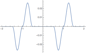
Figure 2: The function $(x,y)\mapsto G_{1}(x,y)-x$.

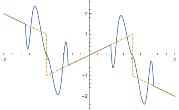
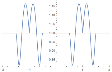
Figure 3: The functions $\tilde{\mu}_{1}$ and $\tilde{\sigma}_{11}$ (blue line) and $\mu_{1}$ and $\sigma_{11}$ (yellow dashed).

We apply Algorithm 3.22 to solve SDE (17). Figure 4 shows the estimated $L^{2}$-error of the approximation of our $G$-transformed Euler-Maruyama method (GM), compared to the Euler-Maruyama (EM) scheme:

$${\operatorname{err}}_{k}:=\log_{2}\left(d\,\sqrt{\hat{E}\left(\left\|X_{T}^{(k)}-X_{T}^{(k-1)}\right\|^{2}\right)}\right)$$

plotted over $\log_{2}\delta^{(k)}$, where $X_{T}^{(k)}$ is the numerical approximation with step size $\delta=\delta^{(k)}$, $\hat{E}$ is an estimator of the mean value using 4096 paths, and $d$ is a normalizing constant so that ${\operatorname{err}}_{1}=\sqrt{1/2}$.

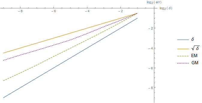
Figure 4: The estimated $L^{2}$-error for the example where $\Theta$ is the unit circle.

We observe that our $G$-transformed (GM) method converges roughly with order $1/2$, and the crude Euler-Maruyama (EM) method seems to converge even at a higher rate. Note however that, even though the Euler-Maruyama method is extensively used in practice, it is not even known whether the method converges strongly for SDEs of the kind considered here. Especially we cannot conclude whether for even smaller step-size the error of the Euler-Maruyama method will still become smaller, will flatten out, or whether it will even explode.

Dividend maximization

In [22] the dividend maximization problem from actuarial mathematics, that is, the problem of maximizing the expected discounted future dividend payments until the time of ruin $\tau$ of an insurance company, is studied. In actuarial mathematics, the solution of this optimization problem serves as a risk measure. The problem is studied in a setup with incomplete information, where the drift of the underlying surplus process of the insurance company from which dividends are paid is driven by an unobservable Markov chain, the states of which represent different phases of the economy; an assumption that makes the model more realistic. In order to solve the optimization problem, the underlying surplus process has to be replaced by a multidimensional process consisting of filter probabilities of the states of the hidden Markov chain and the surplus written in terms of the filter probabilities. The resulting system is

$$dR_{t} =(\bar{\alpha}_{t}-u_{t})\,dt+\beta dW_{t}\,,$$ (18)

$$d\pi_{i}(t) =\left(q_{di}+\sum_{j=1}^{d-1}(q_{ji}-q_{di})\pi_{j}(t)\right)\,dt+\pi_{i}(t)\frac{\alpha_{i}-\bar{\alpha}_{t}}{\beta}\,dW_{t}\,,\quad i=1,\dots,d-1\,,$$

where $\bar{\alpha}_{t}:=\alpha_{d}+\sum_{i=1}^{d-1}(\alpha_{i}-\alpha_{d})\pi_{i}(t)$ and where $(u_{t})_{t\geq 0}\in[0,\bar{u}]$ is the dividend strategy, $R=(R_{t})_{t\geq 0}$ is the surplus process, and the $(\pi_{i}(t))_{t\geq 0}$, $i=1,\dots,d-1$, are the conditional probabilities that the underlying hidden Markov chain is in state $e_{i}$. $W=(W_{t})_{t\geq 0}$ is a one-dimensional Brownian motion. We assume knowledge of the following constants: $(q_{ij})_{i,j=1}^{d}$ are the entries of the intensity matrix of the Markov chain, $\beta$ is the diffusion parameter of the surplus and $\alpha_{i}$, $i=1,\dots,d$, is the drift of the surplus, if the Markov chain is in state $e_{i}$.

The application of filtering theory leads to an equivalent optimization problem:

$$\sup_{u}{\mathbb{E}}_{x,\pi_{1},\dots,\pi_{d-1}}\left(\int_{0}^{\tau}e^{-\delta s}u_{s}\,ds\right)$$ (19)

with discount rate $\delta>0$. This is studied in [22] and the candidate for the optimal dividend policy is of the form $u^{\ast}_{t}=\bar{u}\,{\mathbf{1}}_{[b(\bar{\alpha}_{t}),\infty)}(R_{t})$ with threshold level $b$, leading to a discontinuous drift of the surplus process from which the dividends are paid. Due to the application of filtering theory, the diffusion coefficient is not uniformly elliptic. In order to verify the admissibility of the candidate for the optimal control policy, existence and uniqueness of the underlying state process has to be proven. This can be done by applying the result presented herein and we can also simulate the optimally controlled surplus (e.g., to calculate the expected time of ruin).

And our results are even further applicable: in [22] the optimization problem (19) is solved for $d=2$ by policy iteration in combination with solving an associated partial differential equation. Doing the same for dimension 4 or higher would not be numerically tractable. So in higher dimension one needs to solve the problem by combining policy iteration with simulation.

Figure 5 shows the estimated $L^{2}$-error of the approximation of the solution of (18) in dimension 5 with a linear initial threshold level. In [22] for $d=2$ a threshold level which is a linear interpolation of the constant optimal threshold levels of the problem under full-information was used as an initial policy for policy iteration. However, we need not restrict ourselves to linear threshold levels.

Note that for our example checking whether the non-parallelity condition, Assumption 3.3 holds (in dependence on the parameter choice) is straight-forward.

We see that in this practical example the convergence order is again roughly $1/2$.

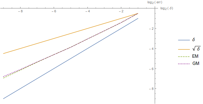
Figure 5: The estimated $L^{2}$-error for the example of dividend maximization.

Further examples from stochastic control theory, where SDEs with discontinuous (and unbounded) drift and degenerate diffusion coefficient appear are, e.g., [16, 20, 21]. The SDEs appearing there can now be shown to have a unique global strong solution under conditions significantly weaker than known so far, and this solution can be approximated with a numerical method that converges with strong order $1/2$. As elaborated above our method can be used for approximating solutions to these optimization problems in dimensions greater than 4, where PDE methods become practically infeasible.

Concluding remarks

In this paper we have presented an existence and uniqueness result of strong solutions for a very general class of SDEs with discontinuous drift und degenerate diffusion coefficient; a class of SDEs that frequently appears in applications when studying stochastic optimal control problems. This is the most general result for such SDEs. Furthermore, we have derived a numerical algorithm that – under the same conditions as for the existence and uniqueness result – is proven to converge and we have established a strong convergence order of $1/2$. We have applied our algorithm to two examples: one of theoretical interest and one coming from a concrete optimal control problem in actuarial mathematics.

Appendix A Supplementary proofs

Proof of Lemma 3.10

Let $\xi\in\Theta$. W.l.o.g. $\xi=0$ and $n(\xi)=e_{d}$, where $e_{d}$ is the $d$-th canonical basis vector of the ${\mathbb{R}}^{d}$. Thus $\Theta$ can locally be parametrized by $\psi:R\longrightarrow{\mathbb{R}}^{d}$ of the form $\psi(y_{1},\ldots,y_{d-1})=(y_{1},\ldots,y_{d-1},\phi(y_{1},\ldots,y_{d-1}))^{\top}$, where $\phi:R\longrightarrow{\mathbb{R}}$ is a $C^{3}$-function with $\phi(0)=0$ and $\phi^{\prime}(0)=0$. Hence, for all $y\in R$,

$$\lambda(y)n(\psi(y)) =\frac{\partial\psi}{\partial y_{1}}(y)\times\dots\times\frac{\partial\psi}{\partial y_{d-1}}(y)$$

$$=\begin{pmatrix}1\\ 0\\ \vdots\\ 0\\ \frac{\partial\phi}{\partial y_{1}}(y)\end{pmatrix}\times\dots\times\begin{pmatrix}0\\ 0\\ \vdots\\ 1\\ \frac{\partial\phi}{\partial y_{d-1}}(y)\end{pmatrix}=\begin{pmatrix}-\frac{\partial\phi}{\partial y_{1}}(y)\\ -\frac{\partial\phi}{\partial y_{2}}(y)\\ \vdots\\ -\frac{\partial\phi}{\partial y_{d-1}}(y)\\ 1\end{pmatrix}\,,$$

with $\lambda(y)=\big{\|}\frac{\partial\psi}{\partial y_{1}}(y)\times\dots\times\frac{\partial\psi}{\partial y_{d-1}}(y)\big{\|}$. Note that $\lambda$ is a $C^{2}$-function satisfying $\lambda^{\prime}(0)=0$ and w.l.o.g. the parametrization is chosen such that $\lambda(0)=1$. Hence

$$\left(\lambda\ n\circ\psi\right)^{\prime}(y) =-\begin{pmatrix}\frac{\partial^{2}\phi}{\partial y_{1}^{2}}(y)&\frac{\partial^{2}\phi}{\partial y_{2}\partial y_{1}}(y)&\dots&\frac{\partial^{2}\phi}{\partial y_{d-1}\partial y_{1}}(y)\\ \frac{\partial^{2}\phi}{\partial y_{1}\partial y_{2}}(y)&\frac{\partial^{2}\phi}{\partial y_{2}^{2}}(y)&\dots&\frac{\partial^{2}\phi}{\partial y_{d-1}\partial y_{2}}(y)\\ \vdots&\vdots&&\vdots\\ \frac{\partial^{2}\phi}{\partial y_{1}\partial y_{d-1}}(y)&\frac{\partial^{2}\phi}{\partial y_{2}\partial y_{d-1}}(y)&\dots&\frac{\partial^{2}\phi}{\partial y_{d-1}^{2}}(y)\\ 0&0&\dots&0\end{pmatrix}=-\begin{pmatrix}H_{\phi}(y)\\ 0\end{pmatrix}\,,$$

where $H_{\phi}(y)$ denotes the Hessian of $\phi$ in $y\in R$. On the other hand $\left(\lambda\ n\circ\psi\right)^{\prime}=n\circ\psi\ \lambda^{\prime}+\lambda\ (n\circ\psi)^{\prime}$. In particular, $(n\circ\psi)^{\prime}(0)=-\left(H_{\phi}(0),0\right)^{\top}$ .

Now choose any $\varepsilon>0$ that is smaller than the reach of $\Theta$. Then $\psi(0)$ is the unique closest point on $\Theta$ both to $\psi(0)+\varepsilon e_{d}$ and $\psi(0)-\varepsilon e_{d}$. In other words, the open balls with centers $\psi(0)+\varepsilon e_{d}$ and $\psi(0)-\varepsilon e_{d}$ contain no point of $\Theta$. Therefore,

$$-\varepsilon(1-\sqrt{1-(\|y\|/\varepsilon)^{2}})\leq\phi(y)\leq\varepsilon(1-\sqrt{1-(\|y\|/\varepsilon)^{2}})$$

for all $y\in R$ with $\|y\|\leq\varepsilon$, from which we conclude that$-\frac{\|y\|^{2}}{\varepsilon}\leq\phi(y)\leq\frac{\|y\|^{2}}{\varepsilon}\,,$ for $\|y\|$ sufficiently small. In particular, we have for $j\neq k$ and sufficiently small $|h|$ that

$$-\frac{2}{\varepsilon}\leq\frac{\phi(h(e_{j}+e_{k}))-\phi(h(e_{j}-e_{k}))}{2h^{2}}\leq\frac{2}{\varepsilon}\,.$$

By letting $h\to 0$ and applying de l’Hospital’s rule twice we see that

$$-\frac{2}{\varepsilon}\leq\frac{\partial^{2}\phi}{\partial y_{j}\partial y_{k}}(0)\leq\frac{2}{\varepsilon}\,.$$

In the same way we conclude from

$$-\frac{1}{\varepsilon}\leq\frac{\phi(he_{j})-\phi(0)+\phi(-he_{j})}{2h^{2}}\leq\frac{1}{\varepsilon}$$

that $-\frac{1}{\varepsilon}\leq\frac{\partial^{2}\phi}{\partial y_{j}^{2}}(0)\leq\frac{1}{\varepsilon}\,.$ Thus

$$\|n^{\prime}(\xi)\|^{2}=\|H_{\phi}(0)\|^{2}\leq\sum_{j=1}^{d-1}\sum_{k=1}^{d-1}\left|\frac{\partial^{2}\phi}{\partial y_{j}\partial y_{k}}(0)\right|^{2}\leq\sum_{j=1}^{d-1}\sum_{k=1}^{d-1}\frac{4}{\varepsilon^{2}}=4\left(\frac{d-1}{\varepsilon}\right)^{2}\,,$$

i.e. $\|n^{\prime}\|$ is bounded by $2\frac{d-1}{\varepsilon}$. Since this holds for all $0<\varepsilon<{\operatorname{reach}}(\Theta)$, we have $\|n^{\prime}\|\leq 2\frac{d-1}{{\operatorname{reach}}(\Theta)}$.

Proof of Lemma 3.11

We prove the claim that a hypersurface that satisfies Assumption 3.2 has the property that every line segment from $x$ to $y$ can be replaced by a continuous curve $\gamma$ from $x$ to $y$ with $\ell(\gamma)<\|x-y\|+\eta$ where $\eta>0$ is a given constant.

Let from now on $\varepsilon<\varepsilon_{0}$, where $\varepsilon_{0}$ is as in Assumption 3.2, so that in particular for every $x\in{\mathbb{R}}^{d}$ with $d(x,\Theta)\leq\varepsilon$ there is a unique closest point $p(x)$ on $\Theta$.

Denote by $s$ the line segment from $x$ to $y$ and identify it with it’s parameter representation $s(t)=x+t(y-x)\|y-x\|^{-1}$. Let $A:=\{t\in[0,\|y-x\|]:s(t)\in\Theta\}$. For any set $S\subseteq{\mathbb{R}}$ denote by $H(S)$ the set of accumulation points of $S$.

Proposition A.1.

Let $t\in H(A)$. Then $n(s(t))\perp s^{\prime}(t)$.

Proof.

Suppose this was not the case, i.e. $n(s(t))\cdot s^{\prime}(t)\neq 0$. W.l.o.g. $n(s(t))\cdot s^{\prime}(t)=C>0$. Let $(t_{j})_{j\in{\mathbb{N}}}$ be a sequence in $A$ with $t_{j}\neq t$, $\lim_{j}t_{j}=t$. W.l.o.g, $t_{j}>t$ for all $j$, or $t_{j}<t$ for all $j$.

By Assumption 3.2 we have $\left(B_{\varepsilon}\left(s(t)-\varepsilon n(s(t))\right)\cup B_{\varepsilon}\left(s(t)+\varepsilon n(s(t))\right)\right)\cap\Theta=\emptyset$, where $B_{r}(z)$ denotes the open ball with midpoint $z$ and radius $r$.

Suppose $t_{j}>t$ for all $j$. Then

$$\|s(t)+\varepsilon n(s(t))-s(t_{j})\|^{2} =\|s(t)-s(t_{j})\|^{2}+2\varepsilon(s(t)-s(t_{j}))\cdot n(s(t))+\varepsilon^{2}\|n(s(t))\|^{2}$$

$$=\|s(t)-s(t_{j})\|^{2}+2\varepsilon(t-t_{j})s^{\prime}(t)\cdot n(s(t))+\varepsilon^{2}$$

$$=|t-t_{j}|^{2}-2\varepsilon|t-t_{j}|C+\varepsilon^{2}$$

$$=|t-t_{j}|(|t-t_{j}|-2\varepsilon C)+\varepsilon^{2}\,,$$

and the last expression is smaller than $\varepsilon^{2}$ for $j$ large enough. Thus we have found a point $\xi$ on $\Theta$, namely $\xi=s(t_{j})$, with $\|\xi-(s(t)+\varepsilon n(s(t)))\|<\|s(t)-(s(t)+\varepsilon n(s(t)))\|=\varepsilon$. But this contradicts the fact that $s(t)$ is the point on $\Theta$ closest to $s(t)+\varepsilon n(s(t))$.

If $t_{j}<t$ for all $j$, then the same argument carries through with $s(t)+\varepsilon n(s(t))$ replaced by $s(t)-\varepsilon n(s(t))$. ∎

Denote the tangent hyperplane on $\Theta$ in the point $\xi$ by $\vartheta(\xi)$, i.e. $\vartheta(\xi)=\xi+\tau(\xi)=\{\xi+b:b\in\tau(\xi)\}$.

Proposition A.2.

For any $\xi\in\Theta$ we can find $r>0$ such that for any $x\in\vartheta(\xi)$ with $\|x-\xi\|<r$ we have that the line segment $\overline{x-\varepsilon n(\xi),x+\varepsilon n(\xi)}$ has precisely one intersection with $\Theta$.

Proof.

We can locally parametrize $\Theta$ by a function on an open environment $V$ of $\xi$ in the tangent hyperplane $\vartheta(\xi)$. That is, there is an open interval $I\subseteq{\mathbb{R}}$ and a $C^{2}$-function $\hat{\psi}:V\longrightarrow I$ such that every point $z\in\{\xi+b+yn(\xi):b\in V,y\in I\}$ can be uniquely written as $z=\xi+b+\hat{\psi}(b)n(\xi)$. Since $\xi\in\vartheta(\xi)$ and thus $\hat{\psi}(\xi)=0$, we may assume that $I=(-\zeta,\zeta)$ for some $0<\zeta<\varepsilon$. Choose some $r$ such that $0<r<\sqrt{\varepsilon^{2}-(\varepsilon-\zeta)^{2}}$ and such that for all $x\in\vartheta(\xi)$ we have $x\in V$ whenever $\|x-\xi\|<r$.

Now if $x\in\vartheta(\xi)$ with $\|x-\xi\|<r$, then precisely one point of $\Theta$ lies on the line segment $\overline{x-\zeta n(\xi),x+\zeta n(\xi)}$. But there is no point of $\Theta$ on the line segment $\overline{x+\zeta n(\xi),x+\varepsilon n(\xi)}$, since this is entirely contained in the open ball $B_{\varepsilon}(\xi+\varepsilon n(\xi))$, which by the unique closest point property for $\xi+\varepsilon n(\xi)$ does not contain any point of $\Theta$.

By the same reasoning $\overline{x-\zeta n(\xi),x-\varepsilon n(\xi)}\cap\Theta=\emptyset$. ∎

Proposition A.3.

Let $\varepsilon_{1}<\varepsilon$. Then for any $y\in{\mathbb{R}}^{d}$ there exists a point $\hat{y}\in{\mathbb{R}}^{d}$ with $d(\hat{y},\Theta)\geq\varepsilon_{1}$ and $\|y-\hat{y}\|\leq\varepsilon_{1}$.

Proof.

If $d(y,\Theta)\geq\varepsilon_{1}$, then set $\hat{y}=y$. Otherwise, there is a unique closest point $p(y)\in\Theta$. Set

$$\hat{y}=\begin{cases}p(y)+\varepsilon_{1}n(p(y))&\text{if }n(p(y))\cdot(y-p(y))>0\\ p(y)-\varepsilon_{1}n(p(y))&\text{if }n(p(y))\cdot(y-p(y))<0\,.\end{cases}$$

Then $\|y-\hat{y}\|\leq\varepsilon_{1}$ is obvious, and $d(\hat{y},\Theta)\geq\varepsilon_{1}$ by the unique closest point property. ∎

We can now modify the straight line from $x$ to $y$ to get a continuous curve, which is not much longer than $\|y-x\|$, but has only finitely many intersections with $\Theta$.

For what follows, let $\alpha\in(0,1)$ and for $0<\delta<\varepsilon$ set $\varepsilon_{1}=\varepsilon-\sqrt{\varepsilon^{2}-\delta^{2}}$.

We construct a sequence $(\gamma_{k})_{k\in{\mathbb{N}}_{0}}$ of continuous curves of finite length which becomes stationary after finitely many steps, i.e. there exists $k_{0}$ such that $\gamma_{k}=\gamma_{k_{0}}$ for all $k\geq k_{0}$.

Furthermore, $\gamma_{k_{0}}$ will have only finitely many intersections with $\Theta$ and it will be only slightly longer than $\|x-y\|$, see (20).

Set $\gamma_{0}=s$.

Step $1$:

If $H(s\cap\Theta)=\emptyset$, then set $\gamma_{1}=\gamma_{0}$.

Otherwise proceed as follows: According to Proposition A.3 there exists a point $\hat{y}$ with $d(\hat{y},\Theta)\geq\varepsilon_{1}$ and $\|y-\hat{y}\|\leq\varepsilon_{1}$. Define $\gamma_{1}$ as the concatenation of the lines $\overline{x,\hat{y}}$ and $\overline{\hat{y},y}$. We have $\ell(\gamma_{1})\leq\|y-x\|+2\varepsilon_{1}$, and there is at most one intersection of $\overline{\hat{y},y}$, the second line segment, with $\Theta$, due to Assumption 3.2. Set $x_{1}=x$.

After step 1 we have constructed a polygonal curve $\gamma_{1}$ such that $\ell(\gamma_{1})\leq\|y-x\|+2\varepsilon_{1}$. If $\gamma_{1}$ has infinitely many intersections with $\Theta$, then all but finitely many are contained in a single line segment, $s_{1}=\overline{x_{1},\hat{y}}$, which satisfies $\ell(s_{1})=\|\hat{y}-x_{1}\|=\|\hat{y}-x\|=\|(y-x)+(\hat{y}-y)\|\leq\|y-x\|+\varepsilon_{1}$.

Now we enter an iteration procedure. Suppose that after $k\geq 1$ steps we have constructed a polygonal curve $\gamma_{k}$, with the properties that $\ell(\gamma_{k})\leq\|y-x\|+2k\varepsilon_{1}$, and such that either $\gamma_{k}$ has finitely many intersections with $\Theta$, or all intersections are contained in a single line segment, $s_{k}=\overline{x_{k},\hat{y}}$, which satisfies $\ell(s_{k})\leq\|y-x\|-(k-1)(\alpha\delta-\varepsilon_{1})+\varepsilon_{1}$.

We construct $\gamma_{k+1}$ from $\gamma_{k}$ as follows:

Step $k+1$:

If $H(\gamma_{k}\cap\Theta)=\emptyset$, then set $\gamma_{k+1}=\gamma_{k}$.

Otherwise, $H(\gamma_{k}\cap\Theta)$ is contained in the line segment $\overline{x_{k},\hat{y}}$. Parametrize this segment by $s_{k}(t)=x_{k}+t\|\hat{y}-x_{k}\|^{-1}(\hat{y}-x_{k})$, $t\in[0,\|\hat{y}-x_{k}\|]$ and let $H_{k}=H\left(\{t:s_{k}(t)\in\Theta\}\right)$.

Set $t_{k}=\min H_{k}$, and let $n_{k}=n(s_{k}(t_{k}))$. If $t_{k}$ is isolated from the left, or if $t_{k}=0$, then set $r_{k}=0$. Now consider the case where $t_{k}$ is not isolated from the left. By Proposition A.1, $s_{k}$ lies in the tangent hyperplane $\vartheta(s_{k}(t_{k}))=s_{k}(t_{k})+\tau(s_{k}(t_{k}))$ and we can find a small ball with radius $r_{k}>0$ such that, for any $t$ with $|t-t_{k}|<r_{k}$, the line segment $\overline{s_{k}(t)-\varepsilon_{1}n_{k},s_{k}(t)+\varepsilon_{1}n_{k}}$ has at most one intersection with $\Theta$, by Proposition A.2.

Consider the line segment $\overline{s_{k}(t_{k}-r_{k})+\varepsilon_{1}n_{k},s_{k}(t_{k}+\alpha\delta)+\varepsilon_{1}n_{k}}$.

If the intersection of this with the plane through $\hat{y}$, which is orthogonal to the line segment, is non-empty, denote the unique intersection point by $z_{k}$.

Then we construct $\gamma_{k+1}$ as the concatenation of the following line segments:

• $\overline{s_{k}(0),s_{k}(t_{k}-r_{k})}$, which by definition of $t_{k}$ and $r_{k}$ has only finitely many intersections with $\Theta$;

• $\overline{s_{k}(t_{k}-r_{k}),s_{k}(t_{k}-r_{k})+\varepsilon_{1}n_{k}}$, which has at most one intersection with $\Theta$ by the construction of $r_{k}$ and Proposition A.2;

• $\overline{s_{k}(t_{k}-r_{k})+\varepsilon_{1}n_{k},z_{k}}$, which is completely contained in $B_{\varepsilon}(s_{k}(t_{k})+\varepsilon n_{k})$, which does not contain any point of $\Theta$ by the unique closest point property for $s_{k}(t_{k})+\varepsilon n_{k}$;

• $\overline{z_{k},\hat{y}}$, which has no intersection with $\Theta$, because as $\|z_{k}-\hat{y}\|=\varepsilon_{1}$, there is no intersection strictly between $z_{k}$ and $\hat{y}$, and $z_{k}$ lies in the closure of $B_{\varepsilon_{1}}(\hat{y})$ (this is where we need Step 1);

• $\overline{\hat{y},y}$.

In this case the curve $\gamma_{k+1}$ has only finitely many intersections with $\Theta$ and $\ell(\gamma_{k+1})=\ell(\gamma_{k})+2\varepsilon_{1}\leq\|y-x\|+2(k+1)\varepsilon_{1}$.

Otherwise, set $x_{k+1}=s_{k}(t_{k}+\alpha\delta)+\varepsilon_{1}n_{k}$, and construct $\gamma_{k+1}$ as the concatenation of the following line segments:

• $\overline{s_{k}(0),s_{k}(t_{k}-r_{k})}$, which by definition of $t_{k}$ and $r_{k}$ has only finitely intersections with $\Theta$;

• $\overline{s_{k}(t_{k}-r_{k}),s_{k}(t_{k}-r_{k})+\varepsilon_{1}n_{k}}$, which has at most one intersection with $\Theta$ by the construction of $r_{k}$ and Proposition A.2;

• $\overline{s_{k}(t_{k}-r_{k})+\varepsilon_{1}n_{k},x_{k+1}}$, which is completely contained in $B_{\varepsilon}(s_{k}(t_{k})+\varepsilon n_{k})$, which does not contain any point of $\Theta$ by the unique closest point property for $s_{k}(t_{k})+\varepsilon n_{k}$;

• $s_{k+1}:=\overline{x_{k+1},\hat{y}}$, which still may have infinitely many intersections with $\Theta$;

• $\overline{\hat{y},y}$.

Again we have that $\ell(\gamma_{k+1})\leq\ell(\gamma_{k})+2\varepsilon_{1}\leq\|y-x\|+2(k+1)\varepsilon_{1}$. Note that

$$\ell(s_{k+1})^{2} =\|x_{k+1}-\hat{y}\|^{2}=\|s_{k}(t_{k}+\alpha\delta)+\varepsilon_{1}n_{k}-\hat{y}\|^{2}$$

$$=\|s_{k}(t_{k}+\alpha\delta)-\hat{y}\|^{2}+\varepsilon_{1}^{2}=(\|s_{k}(t_{k})-\hat{y}\|-\alpha\delta)^{2}+\varepsilon_{1}^{2}\,.$$

In particular, $\|x_{k+1}-\hat{y}\|\leq\big{|}\|s_{k}(t_{k})-\hat{y}\|-\alpha\delta\big{|}+\varepsilon_{1}=\|s_{k}(t_{k})-\hat{y}\|-\alpha\delta+\varepsilon_{1}$. Note that $\|s_{k}(t_{k})-\hat{y}\|-\alpha\delta\geq 0$, since otherwise the line segment $\overline{s_{k}(t_{k}-r_{k})+\varepsilon_{1}n_{k},s_{k}(t_{k}+\alpha\delta)+\varepsilon_{1}n_{k}}$ would intersect the hyperplane orthogonal to $s_{k}$ and passing through $\hat{y}$.

Thus $\|x_{k+1}-\hat{y}\|\leq\|x_{k}-\hat{y}\|-\alpha\delta+\varepsilon_{1}\leq\|x-y\|-k(\alpha\delta-\varepsilon_{1})+\varepsilon_{1}$.

After step $k+1$ we have constructed a polygonal curve $\gamma_{k+1}$ such that $\ell(\gamma_{k+1})\leq\|y-x\|+2(k+1)\varepsilon_{1}$. If $\gamma_{k+1}$ has infinitely many intersections with $\Theta$, then all but finitely many are contained in a single line segment, $s_{k+1}=\overline{x_{k+1},\hat{y}}$, and $\ell(s_{k+1})\leq\|x-y\|-k(\alpha\delta-\varepsilon_{1})+\varepsilon_{1}$.

So finally we have constructed a sequence $(\gamma_{k})_{k\in{\mathbb{N}}_{0}}$ with

• $\ell(\gamma_{k})\leq\|x-y\|+2k\varepsilon_{1}$;

• $\gamma_{k}$ either has only finitely many intersections with $\Theta$, or all but finitely many intersections are contained in a segment of length at most $\|x-y\|-(k-1)(\alpha\delta-\varepsilon_{1})+\varepsilon_{1}$.

Since $\delta<\varepsilon$, we have that $\varepsilon_{1}=\varepsilon-\sqrt{\varepsilon^{2}-\delta^{2}}=\varepsilon\left(1-\sqrt{1-\left(\frac{\delta}{\varepsilon}\right)^{2}}\right)<\frac{\delta^{2}}{\varepsilon}$, such that

$$\alpha\delta-\varepsilon_{1}>\delta\left(\alpha-\frac{\delta}{\varepsilon}\right)>0\,.$$

With this, and since $\|x-y\|-(k-1)(\alpha\delta-\varepsilon_{1})+\varepsilon_{1}\geq\ell(s_{k})\geq 0$, the iteration can have at most

$$k\leq 1+\frac{\|x-y\|+\varepsilon_{1}}{2(\alpha\delta-\varepsilon_{1})}<1+\frac{\|x-y\|+\varepsilon_{1}}{2\delta\left(\alpha-\frac{\delta}{\varepsilon}\right)}<1+\frac{\|x-y\|+\varepsilon}{2\delta\left(\alpha-\frac{\delta}{\varepsilon}\right)}$$

steps before the sequence becomes stationary, and thus there exists a $k_{0}$ such that $\gamma_{k_{0}}$ has at most finitely many intersections with $\Theta$.

For the length of $\gamma_{k}$ for $k\geq k_{0}$ we have

$$\ell(\gamma_{k}) \leq\|x-y\|+2k\varepsilon_{1}\leq\|x-y\|+\left(2\delta+\frac{\|x-y\|+\varepsilon}{\alpha-\frac{\delta}{\varepsilon}}\right)\frac{\delta}{\varepsilon}\,.$$ (20)

This can be made as close to $\|x-y\|$ as we desire by making $\delta$ small. Thus the proof is finished.

G. Leobacher
Institute of Mathematics and Scientific Computing, University of Graz, Heinrichstraße 36, 8010 Graz, Austria
gunther.leobacher@uni-graz.at

M. Szölgyenyi 🖂
Institute of Statistics and Mathematics, Vienna University of Economics and Business, Welthandelsplatz 1, 1020 Vienna, Austria
michaela.szoelgyenyi@wu.ac.at

References

- Berkaoui [2004] A. Berkaoui. Euler Scheme for Solutions of Stochastic Differential Equations with Non-Lipschitz Coefficients. Portugaliae Mathematica, 61(4):461–478, 2004.
- Dudek and Holly [1994] E. Dudek and K. Holly. Nonlinear orthogonal projection. Annales Polonici Mathematici, 59(1):1–31, 1994.
- Étoré and Martinez [2013] P. Étoré and M. Martinez. Exact Simulation for Solutions of One-Dimensional Stochastic Differential Equations Involving a Local Time at Zero of the Unknown Process. Monte Carlo Methods and Applications, 19(1):41–71, 2013.
- Étoré and Martinez [2014] P. Étoré and M. Martinez. Exact Simulation for Solutions of One-Dimensional Stochastic Differential Equations with Discontinuous Drift. ESAIM: Probability and Statistics, 18:686–702, 2014.
- Foote [1984] R. L. Foote. Regularity of the Distance Function. Proceedings of the American Mathematical Society, 92(1):153–155, 1984.
- Gyöngy [1998] I. Gyöngy. A Note on Euler’s Approximation. Potential Analysis, 8:205–216, 1998.
- Halidias and Kloeden [2008] N. Halidias and P. E. Kloeden. A Note on the Euler–Maruyama Scheme for Stochastic Differential Equations with a Discontinuous Monotone Drift Coefficient. BIT Numerical Mathematics, 48(1):51–59, 2008.
- Hutzenthaler et al. [2012] M. Hutzenthaler, A. Jentzen, and P. E. Kloeden. Strong Convergence of an Explicit Numerical Method for SDEs with Nonglobally Lipschitz Continuous Coefficients. The Annals of Applied Probability, 22(4):1611–1641, 2012.
- Itô [1951] K. Itô. On Stochastic Differential Equations. Memoirs of the American Mathematical Society, 4:1–57, 1951.
- Karatzas and Shreve [1991] I. Karatzas and S. E. Shreve. Brownian Motion and Stochastic Calculus. Graduate Texts in Mathematics. Springer-Verlag, New York, second edition, 1991.
- Kloeden and Platen [1992] P. E. Kloeden and E. Platen. Numerical Solutions of Stochastic Differential Equations. Stochastic Modelling and Applied Probability. Springer Verlag, Berlin-Heidelberg, 1992.
- Kohatsu-Higa et al. [2013] A. Kohatsu-Higa, A. Lejay, and K. Yasuda. Weak Approximation Errors for Stochastic Differential Equations with Non-Regular Drift. 2013. Preprint, Inria, hal-00840211.
- Krantz and Parks [1981] S. G. Krantz and H. R. Parks. Distance to Hypersurfaces. Journal of Differential Equations, 40:116–120, 1981.
- Leobacher and Steinicke [2018] G. Leobacher and A. Steinicke. Existence, uniqueness and regularity of the projection onto differentiable manifolds. 2018. arXiv:1811.10578.
- Leobacher and Szölgyenyi [2016] G. Leobacher and M. Szölgyenyi. A Numerical Method for SDEs with Discontinuous Drift. BIT Numerical Mathematics, 56(1):151–162, 2016.
- Leobacher et al. [2014] G. Leobacher, M. Szölgyenyi, and S. Thonhauser. Bayesian Dividend Optimization and Finite Time Ruin Probabilities. Stochastic Models, 30(2):216–249, 2014.
- Leobacher et al. [2015] G. Leobacher, M. Szölgyenyi, and S. Thonhauser. On the Existence of Solutions of a Class of SDEs with Discontinuous Drift and Singular Diffusion. Electronic Communications in Probability, 20(6):1–14, 2015.
- Ruzhansky and Sugimoto [2015] M. Ruzhansky and M. Sugimoto. On Global Inversion of Homogeneous Maps. Bulletin of Mathematical Sciences, 5(1):13–18, 2015.
- Sabanis [2013] S. Sabanis. A Note on Tamed Euler Approximations. Electronic Communications in Probability, 18(47):1–10, 2013.
- Shardin and Szölgyenyi [2016] A. A. Shardin and M. Szölgyenyi. Optimal Control of an Energy Storage Facility Under a Changing Economic Environment and Partial Information. International Journal of Theoretical and Applied Finance, 19(4):1–27, 2016.
- Shardin and Wunderlich [2017] A. A. Shardin and R. Wunderlich. Partially Observable Stochastic Optimal Control Problems for an Energy Storage. Stochastics, 89(1):280–310, 2017.
- Szölgyenyi [2016] M. Szölgyenyi. Dividend Maximization in a Hidden Markov Switching Model. Statistics & Risk Modeling, 32(3-4):143–158, 2016.
- Veretennikov [1981] A. YU. Veretennikov. On Strong Solutions and Explicit Formulas for Solutions of Stochastic Integral Equations. Mathematics of the USSR Sbornik, 39(3):387–403, 1981.
- Veretennikov [1982] A. YU. Veretennikov. On the Criteria for Existence of a Strong Solution of a Stochastic Equation. Theory of Probability and its Applications, 27(3), 1982.
- Veretennikov [1984] A. YU. Veretennikov. On Stochastic Equations with Degenerate Diffusion with Respect to Some of the Variables. Mathematics of the USSR Izvestiya, 22(1):173–180, 1984.
- Zvonkin [1974] A. K. Zvonkin. A Transformation of the Phase Space of a Diffusion Process that Removes the Drift. Mathematics of the USSR Sbornik, 22(129):129–149, 1974.