Strong Cavity-Pseudospin Coupling in Monolayer Transition Metal Dichalcogenides: Spontaneous Spin-Oscillations and Magnetometry

Abstract

Strong coupling between the electronic states of monolayer transition metal dichalcogenides (TMDC) such as MoS₂, MoSe₂, WS₂, or WSe₂, and a two-dimensional (2D) photonic cavity gives rise to several exotic effects. The Dirac type Hamiltonian for a 2D gapped semiconductor with large spin-orbit coupling facilitates pure Jaynes-Cummings type coupling in the presence of a single mode electric field. The presence of an additional circularly polarized beam of light gives rise to valley and spin dependent cavity-QED properties. The cavity causes the TMDC monolayer to act as an on-chip coherent light source and a spontaneous spin-oscillator. In addition, a TMDC monolayer in a cavity is a sensitive magnetic field sensor for an in-plane magnetic field.

Light and matter can become strongly coupled in an optical cavity giving rise to qualitatively new physics and resulting in numerous applications in laser physics, optoelectronics, and quantum information processing. The coherent coupling of light and matter in such systems is described by cavity quantum electrodynamics (QED). The advent of quantum information processing has led to significant activity investigating optical cavity like systems for coherent conversion of qubits between matter or topological states to phonons, photons and circuit oscillators Leibfried et al. (2003); Thompson et al. (1992); Raimond et al. (2001); Hennessy et al. (2007); Kovalev et al. (2014); Soykal et al. (2011); Devoret et al. (1989); Schoelkopf and Girvin (2008); Martinis (2009).

Monolayers and bilayers of transition metal dicalcogenides (TMDCs) couple strongly to light since they are direct bandgap and their large effective masses result in a large density of states and excitonic binding energies Jones et al. (2013); Xu et al. (2014); Jones et al. (2014) . Furthermore, TMDCs have large spin-orbit (SO) coupling resulting in spin-valley polarized valence bands He et al. (2014); Chernikov et al. (2014). The magnetic moment associated with their valley pseudo-spin gives rise to valley-dependent circular dichroism Xu et al. (2014); Jones et al. (2014). Access to these valley and spin degrees of freedom can allow for hybrid on-chip optoelectronic and spintronic devices. Since the spin degrees of freedom for a band are coupled to a particular valley in momentum space, TMDCs might also be candidates for qubits with long coherence times, and there have been suggestions for implementing single qubit gates in TMDC quantum dots Kormányos et al. (2014) and bilayers Gong et al. (2013).

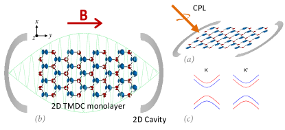
Figure 1: Schematic of a monolayer TMDC in a 2D photonic cavity (a) with an incident beam of circularly polarized light(CPL) to break the valley degeneracy and (b) with an in-plane magnetic field for magnetometry. (c) Sample bandstructure about $K$ and $K^{\prime}$ showing the breaking of the conduction band degeneracy from the effective inplane magnetic field. Colors indicate the band’s spin.

Recent experiments have demonstrated strong coupling effects between 2D materials and photonic cavities. Graphene (Gr) can couple to a photonic crystal’s evanescent modes Gan et al. (2012). It has also been suggested that quantum two level systems (TLSs) can be coupled to surface plasmon modes in graphene Koppens et al. (2011). A Gr/TMDC/Gr heterostructure can be used for photovoltaics Britnell et al. (2013), and an excitonic laser can be created by placing monolayer MoS₂ in a cavity Ye et al. (2015).

In this paper, we show that new properties and device functionalities arise when strong light-matter interaction can be achieved for a gapped 2D Dirac material with strong SO splitting in a 2D optical cavity. 2D cavities are now quite common in circuit-QED Schoelkopf and Girvin (2008). Usually in cavity-QED, the TLS-field coupling occurs via a dipole term or through some nonlinear interactions. Here, the linear k-dependent 2D Dirac type Hamiltonian, after a canonical transformation, directly gives Rabi- or Jaynes-Cummings type coupling between the cavity field and the lattice pseudo-spin. In TMDCs, since the valley and spin indices are coupled, each valley can be selected using circularly polarized light (CPL) of a given handedness Xiao et al. (2012). In a suitable optical cavity this could lead to spontaneous spin oscillations for spintronics. However, CPL flips its handedness upon reflection from a conventional surface – hence it is not easy to design a cavity that will only sustain ether just left- or right-CPL. Some reflective chiral surfaces can suppress this cross polarization Hodgkinson et al. (2002); Maksimov et al. (2014). The evanescent mode of a chiral photonic crystal Konishi et al. (2011) could also be used, but then the TLS-cavity coupling will not be strong.

We suggest a simpler approach and point out an additional advantage of the 2D architecture. In the strongly coupled system of a 2D TMDC monolayer inside a 2D cavity, spontaneous vacuum Rabi oscillations occur even in the absence of photons. However, a 2D cavity only supports linearly polarized electromagnetic vibrational modes. Hence the oscillations occur for both valleys with opposite spin. We propose introducing an additional CPL beam that is incident on the 2D cavity-QED system. Sufficiently intense CPL will select a valley. Since intravalley transitions conserve spin, this leads to pure spin Rabi flopping. In the absence of cavity photons, the spin Rabi oscillations are spontaneous in the strong coupling regime. The vacuum Rabi oscillations for the the spin polarization (SP) of a given valley are amplitude modulated. The overall degree of valley polarization depends on the CPL’s intensity which blue-shifts the Rabi frequency. At higher photon numbers, for a field in a coherent state, the expected collapse and revival type behavior for the Rabi oscillations can be seen. In the absence of a cavity mode that supports CPL, say in a strictly 2D geometry, this device can be used as an on-chip coherent light source and a frequency comb at higher photon number.

This cavity-pseudospin system also has other applications. The system is a highly sensitive sensor of an in-plane magnetic field. An in-plane magnetic field shifts the vacuum Rabi frequency. An extremely encouraging finding is that this frequency shift is scale invariant. Whereas one usually seeks strong cavity-TLS coupling, here the scale invariance suggests high sensitivity even for weak coupling.

Material	$\Lambda_{-}$ (GHz)	$\Lambda_{+}$ (GHz)
MoS2	6.411	5.898
WS2	14.021	10.366
MoSe2	6.128	5.442
WSe2	8.29	6.295

Table 1: Coupling strength or the vacuum Rabi frequency for various TMDCs at zone center. Here $\Lambda_{\pm}$ corresponds to $\omega_{\pm}=E_{g}\pm\Delta_{so}$ transition frequencies. The 2D cavity mode volume($V$) is assumed to be $20\mu m\times 20\mu m\times 100nm$. Note that $\Lambda_{\pm}\propto V^{-1/2}$.

The Model: Consider the Hamiltonian for a monolayer TMDC in an in-plane magnetic field along $y$.

$$H_{o}^{\prime}=H_{o}+H_{b}$$ (1)

$H_{o}$ is the following effective $4\times 4$ two-band $k\cdot p$ Hamiltonian for a given valley,

$$H_{o}=u(\tau\tilde{\sigma}_{x}k_{x}+\tilde{\sigma}_{y}k_{y})+\frac{E_{g}}{2}\tilde{\sigma}_{z}+\frac{\Delta_{so}}{2}\tau s_{z}(\tilde{\sigma}_{z}-I)~{}~{}~{}~{}$$ (2)

where $E_{g}$ is the band gap, $\Delta_{so}$ is the SO splitting and $u$ is the velocity. Here $H_{b}=g\mu_{B}B_{y}s_{y}$ where $g$ is the g-factor and $\mu_{B}$ is the Bhor-magneton. We use $g=-4$ Wang et al. (2015). The Pauli spin matrices along $j$ are $s_{j}$, and $\tilde{\sigma}_{j}$ are the pseudo-spin Pauli matrices in the orbital basis, $\{\psi_{c},\psi_{v}^{\tau}\}=\{\left|d_{z^{2}}\right\rangle,\left|d_{x^{2}+y^{2}}+i\tau d_{xy}\right\rangle\}$. It is implied that $\tilde{\sigma}_{j}=I\otimes\sigma_{j}$ and $s_{j}=\sigma_{j}\otimes I$.

First consider the case of a monolayer-TMDC in a cavity with $B_{y}=0$. For a reflective cavity, with the single-mode of an electric field oscillating along $\hat{x}$, one can canonically transform $k_{x}\rightarrow k_{x}+A_{x}$, where $A_{x}$ is the vector potential along $x$. The TDMC’s coupling Hamiltonian will be $H_{i}=u\tau\sigma_{x}A_{x}(t)=\Lambda\tau\sigma_{x}(a^{*}e^{i\omega t}+ae^{-i\omega t})$ where $\Lambda$ is the coupling constant between the cavity’s electric field and the TMDC bands. Second quantizing the cavity field and making the rotating wave approximation, $\Lambda\sigma_{x}(a^{\dagger}+a)\approx\Lambda(a^{\dagger}\sigma_{-}+a\sigma_{+})$, where $a^{\dagger}(a)$ are the photon creation(annihilation) operators, we obtain a block diagonal Hamiltonian in the dressed orbital state basis. Hence the total system Hamiltonian is

$$H=H_{o}+\frac{\omega}{2}{a^{\dagger}a}+\Lambda\tau(a^{\dagger}\sigma_{-}+a\sigma_{+}).$$ (3)

The complete basis set now consists of the spinor part and the dressed orbital states, $\{[\left|+\right\rangle,\left|-\right\rangle]\otimes[\left|\psi_{c},n\right\rangle,\left|\psi_{v}^{\tau},n+1\right\rangle]\}$. Note that cavity part and the spin part($\left|+\right\rangle,\left|-\right\rangle$) are decoupled in the absence of an external in-plane magnetic field.

We estimate the field coupling constant $\Lambda$ assuming a simple 2D rectangular cavity. The coupling constant for four different TMDCs on resonance are calculated as $\Lambda\propto u\sin(\kappa y)[\epsilon_{o}V(E_{g}\pm\Delta_{so})]^{-\frac{1}{2}}$, where $\kappa$ is the electromagnetic wavevector and $V$ is the mode volume. If $V$ is small, then the coupling will be strong. For the mode volume we assume a nearly-2D rectangular cavity. Hence one can anticipate that strong coupling can be achieved between a 2D TMDC and the cavity. The $\Lambda$s for the two different transitions just for a monolayer TMDC are shown in table.-1.

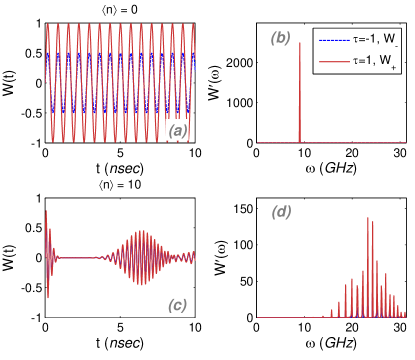
Figure 2: Population inversion for the $\tau=\pm$ valleys showing (a) vacuum Rabi oscillations for $\left\langle n\right\rangle=0$ and (c) collapse and revival of Rabi oscillations for $\left\langle n\right\rangle=10$ for a field initially in a coherent state. The corresponding power spectra, $\mathcal{W}^{\prime}(\omega)=\int|{\mathcal{W}}(t)|^{2}e^{i\omega t}dt$, is shown in (b) and (d). Here the drive is $\omega=E_{g}-\Delta_{so}$, and the circularly polarized light has $\left\langle{E}\right\rangle=\Lambda$.

The direct product of the photon state and the valance band wavefunction at initial time $t=0$ is $\Psi_{\pm,{\bf k}}^{\tau,v}=\sum C_{n}|\psi_{v}^{\tau};\pm;n\rangle$. where $|C_{n}|^{2}$ is the probability distribution number of $n$ photons. The wavefunction at time $t$ is obtained by time evolving with $U=\exp(-iHt)$.

Since the two valleys do not couple with each other one can only consider intravalley optical effects in the present model. For a given valley, in the absence of an external magnetic field, the valance to conduction band(CB) population inversion in the cavity is

$$\mathcal{W^{\tau}_{\pm}}({\bf k})=\displaystyle\sum_{n}\left|C_{n}\right|^{2}\left(\vartheta_{\pm}\cos(\frac{\nu^{\tau}_{\pm}t}{2})+\varphi_{\pm}\sin(\frac{\nu^{\tau}_{\pm}t}{2})\right),$$ (4)

where

$$\vartheta_{\pm} =\frac{1+(\mathcal{E_{\pm}}^{2}-\mathcal{L}_{\pm}^{2})}{[(1+(\mathcal{E_{\pm}}+\mathcal{L}_{\pm})^{2})(1+(\mathcal{E_{\pm}}-\mathcal{L}_{\pm})^{2})]^{1/2}}$$

$$\varphi_{\pm} =\frac{w_{\pm}(\mathcal{E_{\pm}}+\mathcal{L}_{\pm})+w_{\pm}^{*}(\mathcal{E_{\pm}}-\mathcal{L}_{\pm})+f_{\pm}(\mathcal{E_{\pm}}^{2}-\mathcal{L}_{\pm}^{2}-1)}{[(1+(\mathcal{E_{\pm}}+\mathcal{L}_{\pm})^{2})(1+(\mathcal{E_{\pm}}-\mathcal{L}_{\pm})^{2})]^{1/2}}$$

$$\mathcal{E_{\pm}} ={(E_{g}\pm{\tau}\Delta_{so})}/{2({\tau k_{x}^{\prime}+ik_{y}^{\prime}})}$$

$$\mathcal{L_{\pm}} ={\sqrt{\left({E_{g}}\pm{{\tau}\Delta_{so}}\right)^{2}+4(k_{x}^{\prime 2}+k_{y}^{\prime 2})}}/{2(\tau k_{x}^{\prime}+ik_{y}^{\prime})}.$$

Here $\Lambda_{n}=\Lambda\sqrt{1+n}$, $k^{\prime}_{x(y)}=uk_{x(y)}$, $\Omega^{\tau}_{\pm}=E_{g}\pm{\tau}\Delta_{so}-\omega$, $\nu^{\tau}_{\pm}=\sqrt{(\Omega^{\tau}_{\pm})^{2}+(\tau k^{\prime}_{x}+{\tau}\Lambda_{n})^{2}+k_{y}^{\prime 2}}$, $f_{\pm}={\Omega^{\tau}_{\pm}}/{\nu^{\tau}_{\pm}}$ and $w_{\pm}={(\tau\Lambda_{n}+\tau k_{x}^{\prime}-ik_{y}^{\prime})}/{\nu^{\tau}_{\pm}}$. The $\pm$ signs represent different spin states. Since these transitions are also $\bf k$ dependent, the overall inversion probability is obtained after integrating over $\bf k$, $\mathcal{W}^{\tau}_{\pm}=\displaystyle\int\mathcal{W^{\tau}_{\pm}}({\bf k})d{\bf k}$.

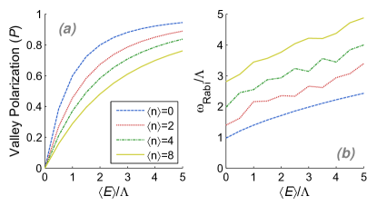
Figure 3: (a) Valley polarization inside a cavity as a function of CPL intensity and for different photon numbers. (b) Peak Rabi frequency shift as a function of CPL intensity. The cavity’s resonance frequency is $\omega=E_{g}-\Delta_{so}$.

Valley Selectable Photonic Spin Oscillator: In the absence of $B_{y}$, in a monolayer TMDC, only interband transitions between bands of the same spin are allowed. We assume that the single cavity mode is initially in a coherent state, $|C_{n}|^{2}=\exp(-\langle n\rangle)\frac{{\langle n\rangle}^{n}}{n!}$ where $\langle{n}\rangle$ is the average photon number.

For a drive resonant with the gap, $\omega=E_{g}-\Delta_{so}$, the vacuum Rabi oscillations are shown in Fig. 2(a) along with the corresponding Fourier spectra in Fig. 2(b). For $\langle{n}\rangle=0$ there is spontaneous emission and Rabi flipping for the TLS. For the opposite spin states (with gap $E_{g}+\Delta_{so}$), the maximum Rabi oscillation amplitude $\sim 0$ since $\omega$ is off-resonance with this transition.

The valley dependent Rabi oscillations are shown in Fig. 2. These are pure spin oscillations from the cavity coupling. A bias for a particular valley (hence spin) is created by using CPL of a given handedness. We use an additional canonical transformation for introducing CPL, $k^{\prime}_{x}\rightarrow k^{\prime}_{x}+\left\langle{E}_{x}\right\rangle$ and $k^{\prime}_{y}\rightarrow k^{\prime}_{y}\pm i\left\langle{E}_{y}\right\rangle$ where, $\left\langle{E}_{x}\right\rangle=\left\langle{E}_{y}\right\rangle=\left\langle{E}\right\rangle$ and $\left\langle{E}\right\rangle$ is the time averaged field. Right-CPL favors the $\tau=1$ valley as shown in Fig. 2 since it biases the Hamiltonian by adding a $\left\langle{E}_{x}\right\rangle\tau\tilde{\sigma}_{x}+i\left\langle{E}_{y}\right\rangle\tilde{\sigma}_{y}$ term.

When $\langle{n}\rangle>0$, the Rabi oscillations undergo collapse and revival (CR) which are more rapid, more distinct, and temporally spaced further apart with increasing $\left\langle n\right\rangle$. Each term in the summation over $n$ represents Rabi flips weighted by $C_{n}$, which are all correlated at $t=0$. However, at longer times the destructive interference between the weighted terms leads to the collapses and then constructive interference leads to revivals. Fig. 2(c) shows that this purely quantum mechanical CR feature can be individually observed for each valley. This CR happens even in the presence of CPL, but the amplitude of the CRs are inequivalent for each valley, and they continue indefinitely with each revival being smaller in amplitude and less distinct from the preceding collapse. The Fourier spectra shows a frequency comb type behavior, where the number of spectral peaks is $\propto\left\langle n\right\rangle$. In the present treatment CPL blue-shifts the central Rabi frequency peak, which is discussed in greater detail next.

The valley(spin) polarization in this system can be characterized as follows,

$$\mathcal{P}=\frac{|\mathcal{W}^{\tau=1}_{+}|^{2}_{max}-|\mathcal{W}^{\tau=-1}_{-}|^{2}_{max}}{|\mathcal{W}^{\tau=1}_{+}|^{2}_{max}+|\mathcal{W}^{\tau=-1}_{-}|^{2}_{max}}.$$ (5)

The degree of valley polarization depends on the CPL’s intensity $\left\langle\mathcal{E}\right\rangle$ as shown in Fig. 3(a). As $\left\langle\mathcal{E}\right\rangle$ is increased $\mathcal{P}$ tends towards 1, but it also tends to saturate. For a given $\left\langle\mathcal{E}\right\rangle$, $\mathcal{P}$ is higher for smaller $\left\langle n\right\rangle$. This is because the cavity photons are also vibrating along $x$ which will tend to make the incident light more elliptically polarized as $\left\langle n\right\rangle$ is increased. Increasing $\left\langle\mathcal{E}\right\rangle$ also shifts the central Rabi frequency peak towards higher frequencies as shown in Fig. 3(b), since CPL increases the effective $\Lambda$ (see $\nu_{\pm}^{\tau}$). The slope $d\mathcal{P}/d\left\langle\mathcal{E}\right\rangle$ is roughly the same for all $\left\langle n\right\rangle$ as expected.

A spin-Zeeman field along $z$ does not affect any of these results, since it simply adds a phase factor. For fields up to $1$ T the valley Zeeman effect Aivazian et al. (2015) also does not do much although it polarizes the valleys. The addition of an inplane magnetic field $B_{y}$ however leads to level detuning and leakages – but again it does not affect the overall $\mathcal{P}$ for this system for fields up to $1$ T. However the inclusion of $B_{y}$ in this 2D cavity-QED system reveals a key technological application.

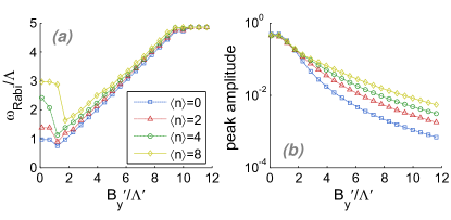
Figure 4: (a) Normalized peak Rabi frequency as a function of the normalized magnetic field for different photon numbers. (b) Corresponding peak oscillation amplitude for the population transfer between valance- and conduction band states with the same spin for the $\tau=1$ valley. The drive $\omega=E_{g}-\Delta_{so}$, $\Lambda^{\prime}=\hbar\Lambda$ and $B^{\prime}_{y}=g\mu_{B}B_{y}$.

Application as a Magnetometer: A monolayer TMDC in an optical cavity can be used for sensitive magnetic field sensing applications. For a 2D material, $B_{y}$ only affects the spin states and does not lead to the formation of Landau levels. However, now the two orbital TLSs are not deoupled anymore and the dynamics of this system is significantly altered in the presence of $B_{y}$. We numerically calculate the population transfer probabilities in the $4\times 4$ the dressed state basis.

The magnetic field modifies the zone center energies to $E_{g}/2\pm B_{y}$ and $-E_{g}/2\mp\sqrt{B_{y}^{2}+\Delta_{so}^{2}}$, which leads to level detuning. This leads to an increase in the Rabi oscillation frequency and a decrease in the oscillation amplitude. The peak Rabi-flop frequencies normalized to $\Lambda$ are shown as a function of $B_{y}/\Lambda$ for different photon numbers for the drive $\omega=E_{g}-\Delta_{so}$ in Fig. 4.

At low $B_{y}$, $\omega_{peak}$ does not change much. And at higher $B_{y}$, $\omega_{peak}$ saturates. However the results in the intermediate regime are extremely encouraging. First, the linear scaling of $\omega_{peak}$ with $B_{y}$, and the invariance of this linear scaling and its slope with $B_{y}/\Lambda$ implies that this device can be used as a very sensitive magneto-meter.

This is a key result. For most cavity-QED applications such as lasing, very strong coupling is desired. Here because of the invariance as a function of $B_{y}/\Lambda$ one could get to very small magnetic field sensing limits. This is only possible because of the unique combination of a gapped material with large SO interactions in a 2D geometry – all of which are necessary. The direct gap makes the system optically active and the 2D geometry allows $B_{y}$ to couple to spin without introducing unwanted Landau levels which then subsequently couples the CB orbitals.

In theory these effects can be reproduced if one just added a $B_{y}\sigma_{y}$ term to the Jaynes-Cummings Hamiltonian. But physically one cannot have an electric dipole coupling and a magnetic field coupling in the same matrix element for an orbital two-level-system. We also argue that this would be robust even with cavity imperfections and spin-dephasing and relaxation as one is not concerned with the decay of the signal, but just with the main peak Fourier component. Experimentally this would amount to spectrally decomposing the time dependent photo-luminescence signal.

Unusual Conduction Band Transitions: In the presence of $B_{y}$, either direct or indirect transitions between all four states in a valley are allowed. However some rather peculiar features stand out for the CB $\psi_{c,-}\leftrightarrow\psi_{c,+}$ transitions. The Rabi flops for these transitions are shown in Fig. 5. These results were obtained exactly by numerically projecting $U=\exp(-iHt)$ between the dressed CB eigenstates of $H_{o}^{\prime}$. At very small but finite $B_{y}$, the vacuum Rabi flops reach 1. As the magnetic field strength increases, the amplitude decreases, but the Rabi frequency does not shift. But again if $B_{y}=0$, this Rabi flipping would vanish.

In general $[H_{0},H_{b}]\neq 0$, however to gain a more intuition one can approximate $U\approx e^{-iHt}e^{-iH_{b}t}$, which is valid for small $B_{y}$. Then the CB population inversion is

$$\left\langle\Psi_{-}^{c}\right|U\left|\Psi_{+}^{c}\right\rangle \sim\cos(B_{y}t)(\mathcal{W^{\prime}}_{+}-\mathcal{W^{\prime}}_{-})$$

$$+i\sin(B_{y}t)(\mathcal{C}_{+}\mathcal{W^{\prime}}_{+}-\mathcal{C}_{-}\mathcal{W^{\prime}}_{-})$$ (6)

where $\mathcal{C}_{\pm}=(\sqrt{B_{y}^{2}+\Delta_{so}^{2}}\pm\tau\Delta_{so})/B_{y}$ and $\mathcal{W^{\prime}}_{\pm}=\sum|C_{n}|^{2}\left(\cos(\frac{\nu_{\pm}t}{2})+\frac{\Omega_{\pm}}{\nu_{\pm}}\sin(\frac{\nu_{\pm}t}{2})\right)$. Eq. 6 approaches 1 in the limit of a vanishing $B_{y}$. The peculiar Rabi flopping in Fig. 5 can be explained as follows. In the absence of a magnetic field, the CB $c_{\pm}$ states are degenerate but are completely decoupled from each other in the present $k\cdot p$ model. An infinitesimally small $B_{y}$ lifts this degeneracy and couples the two CB states allowing $\Psi^{c}_{-}\leftrightarrow\Psi^{c}_{+}$ transitions. However now since the two levels are still nearly degenerate for a small $B_{y}$, there is an almost perfect overlap of the wavefunctions. As a result the Rabi flops reach 1 for infinitesimally small $B_{y}$s.

Eq. 6 reproduces this behavior in the limit of small $B_{y}$. As the magnetic field strength increases, the amplitude decreases, but the Rabi frequency does not shift. For $\left\langle n\right\rangle=10$, the CR type behavior is seen for these states also.

It should be noted that in actual TMDC monolayers, the CB states are also non-degenerate and spin-split, although the spin splitting is much less than that of the valence band Zibouche et al. (2014); Kormányos et al. (2014, 2015). While this CB splitting does not affect the other results, the CB population transfer amplitudes would less than what is shown in Fig. 5. Overall, this is an important effect to take into account when considering quantum information processing applications.

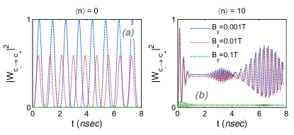
Figure 5: Population transfer between the conduction band states with opposite spin $\psi_{c,-}\leftrightarrow\psi_{c,+}$ shown for two different photon numbers and magnetic fields. The drive is at $\omega=E_{g}-\Delta_{so}$.

In summary we show that the strong coupling between the lattice pseudo-spin of an inversion asymmetric monolayer TMDC and a photonic cavity leads to a number of physical effects. This system can act as an on-chip coherent light source. The Dirac type Hamiltonian for a 2D gapped semiconductor with a large SO interaction facilitates pure Jaynes-Cummings coupling in the presence of a single mode electric field. This gives rise to valley and spin dependent optical properties which can be controlled in a 2D architecture by using an additional CPL field. With CPL, the strong coupling effect leads to a spontaneous spin-oscillator with zero cavity photons! For a higher photon number coherent state field, valley selective collapse and revival of Rabi oscillations occur.

The presence of an external in-plane magnetic field leads to a number of additional effects. This TMDC cavity-QED device can be used for sensitive magnetic field sensing applications, which is only possible here because of the combination of a gapped 2D material with large SO interactions in a cavity. A consequence of an inplane magnetic field is that Rabi oscillations between opposite CB spin states become feasible in a monolayer-TMDC. These oscillations are robust for small magnetic field fluctuations which could also be useful for quantum information applications.

Acknowledgements: This work was supported by FAME, one of six centers of STARnet, a Semiconductor Research Corporation program sponsored by MARCO and DARPA and the NSF 2-DARE, EFRI-143395.

References

- Leibfried et al. (2003) D. Leibfried, R. Blatt, C. Monroe, and D. Wineland, Rev. Mod. Phys. 75, 281 (2003).
- Thompson et al. (1992) R. J. Thompson, G. Rempe, and H. J. Kimble, Phys. Rev. Lett. 68, 1132 (1992).
- Raimond et al. (2001) J. M. Raimond, M. Brune, and S. Haroche, Rev. Mod. Phys. 73, 565 (2001).
- Hennessy et al. (2007) K. Hennessy, A. Badolato, M. Winger, D. Gerace, M. Atature, S. Gulde, S. Falt, E. L. Hu, and A. Imamoglu, Nature 445, 896 (2007).
- Kovalev et al. (2014) A. A. Kovalev, A. De, and K. Shtengel, Phys. Rev. Lett. 112, 106402 (2014).
- Soykal et al. (2011) O. O. Soykal, R. Ruskov, and C. Tahan, Phys. Rev. Lett. 107, 235502 (2011).
- Devoret et al. (1989) M. H. Devoret, D. Esteve, J. M. Martinis, and C. Urbina, Physica Scripta 1989, 118 (1989).
- Schoelkopf and Girvin (2008) R. J. Schoelkopf and S. M. Girvin, Nature 451, 664 (2008).
- Martinis (2009) J. M. Martinis, Quantum Information Processing 8, 81 (2009).
- Jones et al. (2013) A. M. Jones, H. Yu, N. J. Ghimire, S. Wu, G. Aivazian, J. S. Ross, B. Zhao, J. Yan, D. G. Mandrus, D. Xiao, et al., Nature nanotechnology 8, 634 (2013).
- Xu et al. (2014) X. Xu, W. Yao, D. Xiao, and T. F. Heinz, Nature Physics 10, 343 (2014).
- Jones et al. (2014) A. M. Jones, H. Yu, J. S. Ross, P. Klement, N. J. Ghimire, J. Yan, D. G. Mandrus, W. Yao, and X. Xu, Nature Physics 10, 130 (2014).
- He et al. (2014) K. He, N. Kumar, L. Zhao, Z. Wang, K. F. Mak, H. Zhao, and J. Shan, Phys. Rev. Lett. 113, 026803 (2014).
- Chernikov et al. (2014) A. Chernikov, T. C. Berkelbach, H. M. Hill, A. Rigosi, Y. Li, O. B. Aslan, D. R. Reichman, M. S. Hybertsen, and T. F. Heinz, Phys. Rev. Lett. 113, 076802 (2014).
- Kormányos et al. (2014) A. Kormányos, V. Zólyomi, N. D. Drummond, and G. Burkard, Phys. Rev. X 4, 011034 (2014).
- Gong et al. (2013) Z. Gong, G.-B. Liu, H. Yu, D. Xiao, X. Cui, X. Xu, and W. Yao, Nature communications 4, 2053 (2013).
- Gan et al. (2012) X. Gan, K. F. Mak, Y. Gao, Y. You, F. Hatami, J. Hone, T. F. Heinz, and D. Englund, Nano letters 12, 5626 (2012).
- Koppens et al. (2011) F. H. Koppens, D. E. Chang, and F. J. Garcia de Abajo, Nano letters 11, 3370 (2011).
- Britnell et al. (2013) L. Britnell, R. Ribeiro, A. Eckmann, R. Jalil, B. Belle, A. Mishchenko, Y.-J. Kim, R. Gorbachev, T. Georgiou, S. Morozov, et al., Science 340, 1311 (2013).
- Ye et al. (2015) Y. Ye, Z. J. Wong, X. Lu, H. Zhu, X. Chen, Y. Wang, and X. Zhang, Nature Photonics , 733–737 (2015).
- Xiao et al. (2012) D. Xiao, G.-B. Liu, W. Feng, X. Xu, and W. Yao, Phys. Rev. Lett. 108, 196802 (2012).
- Hodgkinson et al. (2002) I. J. Hodgkinson, M. Arnold, M. W. McCall, A. Lakhtakia, et al., Optics communications 210, 201 (2002).
- Maksimov et al. (2014) A. A. Maksimov, I. I. Tartakovskii, E. V. Filatov, S. V. Lobanov, N. A. Gippius, S. G. Tikhodeev, C. Schneider, M. Kamp, S. Maier, S. Höfling, and V. D. Kulakovskii, Phys. Rev. B 89, 045316 (2014).
- Konishi et al. (2011) K. Konishi, M. Nomura, N. Kumagai, S. Iwamoto, Y. Arakawa, and M. Kuwata-Gonokami, Phys. Rev. Lett. 106, 057402 (2011).
- Wang et al. (2015) G. Wang, L. Bouet, M. M. Glazov, T. Amand, E. L. Ivchenko, E. Palleau, X. Marie, and B. Urbaszek, 2D Materials 2, 034002 (2015).
- Aivazian et al. (2015) G. Aivazian, Z. Gong, A. M. Jones, R.-L. Chu, J. Yan, D. G. Mandrus, C. Zhang, D. Cobden, W. Yao, and X. Xu, Nature Physics , 148–152 (2015).
- Zibouche et al. (2014) N. Zibouche, A. Kuc, J. Musfeldt, and T. Heine, Ann. Phys. (Berlin) 526, 395 (2014).
- Kormányos et al. (2015) A. Kormányos, G. Burkard, M. Gmitra, J. Fabian, V. Zólyomi, N. D. Drummond, and V. Fal’ko, 2D Materials 2, 022001 (2015).