Transformations and Hardy-Krause variation

Abstract

Using a multivariable Faa di Bruno formula we give conditions on transformations $\tau:[0,1]^{m}\to{\cal X}$ where ${\cal X}$ is a closed and bounded subset of ^d such that $f\circ\tau$ is of bounded variation in the sense of Hardy and Krause for all $f\in C^{d}({\cal X})$. We give similar conditions for $f\circ\tau$ to be smooth enough for scrambled net sampling to attain $O(n^{-3/2+\epsilon})$ accuracy. Some popular symmetric transformations to the simplex and sphere are shown to satisfy neither condition. Some other transformations due to Fang and Wang (1993) satisfy the first but not the second condition. We provide transformations for the simplex that makes $f\circ\tau$ smooth enough to fully benefit from scrambled net sampling for all $f$ in a class of generalized polynomials. We also find sufficient conditions for the Rosenblatt-Hlawka-Mück transformation in ² and for importance sampling to be of bounded variation in the sense of Hardy and Krause.

1 Introduction

Quasi-Monte Carlo (QMC) sampling is usually applied to integration problems over the domain $[0,1]^{d}$. Other domains, such as triangles, disks, simplices, spheres, balls, et cetera are also of importance in applications. Monte Carlo (MC) sampling over such a domain ${\mathcal{X}}\subset{}^{d}$ is commonly done by finding a uniformity preserving transformation $\tau:[0,1]^{m}\to{\mathcal{X}}$. Such transformations yield $\boldsymbol{x}=\tau(\boldsymbol{u})\sim\mathbf{U}({\mathcal{X}})$ when $\boldsymbol{u}\sim\mathbf{U}[0,1]^{m}$ so that

$$\frac{1}{{\mathbf{vol}}({\mathcal{X}})}\int_{{\mathcal{X}}}f(\boldsymbol{x})\mathrm{\,d}\boldsymbol{x}=\int_{[0,1]^{m}}f(\tau(\boldsymbol{u}))\mathrm{\,d}\boldsymbol{u}.$$ (1)

Then we estimate $\mu=\int_{{\cal X}}f(\boldsymbol{x})\mathrm{\,d}\boldsymbol{x}$ by $({\mathbf{vol}}({\cal X})/n)\sum_{i=1}^{n}f(\tau(\boldsymbol{u}_{i}))$ for $\boldsymbol{u}_{i}{\stackrel{{\scriptstyle\mathrm{iid}}}{{\sim}}}\,\mathbf{U}[0,1]^{d}$. We will often take ${\mathbf{vol}}({\cal X})=1$ for simplicity.

A very standard approach to QMC sampling of such domains is to employ the same transformation $\tau$ as in MC, but to replace independent random $\boldsymbol{u}_{i}$ by QMC or randomized QMC (RQMC) points. The uniformity-preserving transformation $\tau$ satisfies equation (1) when $m=d$ and $\tau$ has a Jacobian determinant everywhere equal to $1/{\mathbf{vol}}({\mathcal{X}})=1$. It also holds when that Jacobian determinant is piecewise constant and equal to $\pm 1$ at all $\boldsymbol{u}$. Equation (1) does not require $m=d$. For instance, in Section 5.1, we study a logarithmic mapping from $[0,1]^{3}$ to a two-dimensional equilateral triangle which satisfies (1).

When the function $f\circ\tau$ is of bounded variation in the sense of Hardy and Krause (BVHK), then the Koksma-Hlawka inequality applies and QMC can attain the convergence rate $O(n^{-1+\epsilon})$. Under additional smoothness conditions on $f\circ\tau$, certain RQMC methods (scrambled nets) have a root mean squared error (RMSE) of $O(n^{-3/2+\epsilon})$.

The paper proceeds as follows. Section 2 gives a sufficient condition for a function $f$ on $[0,1]^{d}$ to be in BVHK and a stronger condition for that function to be integrable with RMSE $O(n^{-3/2+\epsilon})$ by scrambled nets. Those conditions are expressed in terms of certain partial derivatives of $f$. Section 3 considers how to apply the conditions from Section 2 to compositions $f\circ\tau$. There are good sufficient conditions for compositions of single variable functions to be in BVHK, but the multivariate setting is more complicated as shown by a counterexample there. Then we specialize a multivariable Faa di Bruno formula from Constantine and Savits, (1996) to the mixed partial derivatives required for QMC. Section 4 gives sufficient conditions for $f\circ\tau$ to be in BVHK and also for it to be smooth enough for scrambled nets to improve on the QMC rate. There is also a discussion of necessary conditions. We stipulate there that at least the components of $\tau$ should themselves be in BVHK. Section 5 considers two widely used transformations $\tau$ that are symmetric operations on $d$ input variables to yield uniform points in the $d-1$ dimensional simplex and sphere respectively. Unfortunately some components of $\tau$ fail to be in BVHK for these transformations. Section 6 shows that some classic mappings to the simplex, sphere and ball from Fang and Wang, (1993) are in BVHK, although they are not smooth enough to benefit from RQMC. Section 7 considers non-uniform transformations including importance sampling, Rosenblatt-Hlawka-Mück sequential inversion, and a non-uniform transformation on the unit simplex that yields the customary RQMC convergence rate for a class of functions including all polynomials on the simplex.

While finishing up this paper we noticed that Cambou et al., (2015) have also applied the Faa di Bruno formula in a QMC application, though they apply it to a different set of problems. They use it to give sufficient conditions for some integrands with respect to copulas to be in BVHK. They extend Hlawka and Mück, (1972) for inverse CDF sampling to some copulas with mixed partial derivatives that are singular on the boundaries of the unit cube. They closely study the Marshall-Olkin algorithm which generates points from a $d$ dimensional Archimedean copula from a point in $[0,1]^{d+1}$ and give conditions for quadrature errors to be bounded by a multiple of the $d+1$-dimensional discrepancy and weaker conditions for a bound $\log(n)$ times as large as that.

2 Smoothness conditions

Quasi-Monte Carlo sampling attains an error rate of $O(n^{-1}(\log n)^{d-1})$, if the function $f\in{\mathrm{BVHK}}$. Here we give a simply checked sufficient condition for $f\in{\mathrm{BVHK}}$. We use ${\mathrm{V}_{\mathrm{HK}}}(f)$ for the total variation of $f$ in the sense of Hardy and Krause and ${\mathrm{V}_{\mathrm{IT}}}(f)$ for the total variation of $f$ in the sense of Vitali.

Let $1{:}d=\{1,2,\dots,d\}$. For a set $u\subseteq 1{:}d$, let $|u|$ denote the cardinality of $u$ and $-u=1{:}d\setminus u$ its complement. Let $\partial^{u}f$ denote the partial derivative of $f$ taken once with respect to each variable $j\in u$. By convention $\partial^{\varnothing}f=f$. For $\boldsymbol{x}\in[0,1]$ and $u\subseteq 1{:}d$ let $\boldsymbol{x}_{u}{:}{\boldsymbol{1}}_{-u}$ be the point $\boldsymbol{y}\in[0,1]^{d}$ with $y_{j}=x_{j}$ for $j\in u$ and $y_{j}=1$ for $j\not\in u$.

If the mixed partial derivative $\partial^{1:d}f$ exists then

$${\mathrm{V}_{\mathrm{IT}}}(f) \leqslant\int_{[0,1]^{d}}|\partial^{1{:}d}f(\boldsymbol{x})|\mathrm{\,d}\boldsymbol{x},\quad\text{and}$$ (2)

$${\mathrm{V}_{\mathrm{HK}}}(f) \leqslant\sum_{u\neq\varnothing}\int_{[0,1]^{|u|}}|\partial^{u}f(\boldsymbol{x}_{u}{:}{\boldsymbol{1}}_{-u})|\mathrm{\,d}\boldsymbol{x}_{u}.$$ (3)

These and related results are presented in Owen, (2005). Fréchet, (1910) shows that the Vitali bound (2) becomes an equality if $\partial^{1{:}d}f$ is continuous on $[0,1]^{d}$. The Hardy-Krause variation is a sum of Vitali variations for which (3) arises by applying (2) term by term.

For scrambled nets, a kind of RQMC, to attain a root mean squared error of order $O(n^{-3/2}(\log n)^{(d-1)/2})$ the function $f$ must be smooth in the following sense:

$$\|\partial^{u}f\|^{2}_{2}\equiv\int(\partial^{u}f(\boldsymbol{x}))^{2}\mathrm{\,d}\boldsymbol{x}<\infty,\quad\forall u\subseteq 1{:}d.$$ (4)

For a description of digital nets including scramblings of them see Dick and Pillichshammer, (2010). Two scramblings with RMSE of $O(n^{-3/2+\epsilon})$ are the nested uniform scramble in Owen, (1995) and the nested linear scramble of Matoušek, (1998). Geometric nets and scrambled geometric nets have been introduced in Basu and Owen, 2015b for sampling uniformly on ${\cal X}^{s}$ where ${\cal X}$ is a closed and bounded subset of ^d. Scrambled geometric nets attain an RMSE of $O(n^{-1/2-1/d}(\log n)^{(s-1)/2})$ for certain smooth functions defined on ${\cal X}^{s}$. The construction of scrambled geometric nets is based on the recursive partitions used by Basu and Owen, 2015a to sample the triangle.

We will study transformations by considering which combinations of $f$ and $\tau$ give ${\mathrm{V}_{\mathrm{HK}}}(f\circ\tau)<\infty$. For such combinations plain QMC will be asymptotically better than geometric nets when $s=1$ and $d\geqslant 3$. Similarly, if $\partial^{u}(f\circ\tau)\in L^{2}$ for all $u\subseteq 1{:}d$, then scrambled nets are asymptotically better than geometric nets for $d\geqslant 2$.

Higher order digital nets (Dick,, 2009) achieve even better rates of convergence than plain (R)QMC does, but they require even stronger smoothness conditions. Their randomized versions (Dick,, 2011) further increase accuracy (in root mean square) under yet stronger smoothness conditions.

3 Function composition

We would like a condition under which the composition $f\circ\tau:[0,1]^{m}\to{}^{d}\to\real$ is in BVHK. For the case $d=m=1$, BVHK for $f\circ\tau$ reduces to ordinary BV. Josephy, (1981) gives a very complete characterization of when compositions of one dimensional functions are in BV.

Let $f$ and $\tau$ be functions of bounded variation from $[0,1]$ to $[0,1]$. Theorem 4 of Josephy, (1981) shows that $f\circ\tau\in{\mathrm{BV}}$ holds for all $\tau\in{\mathrm{BV}}$ if and only if $f$ is Lipschitz. The statement on $\tau$ is a bit more complicated. His Theorem 3 shows that $f\circ\tau\in{\mathrm{BV}}$ for all $f\in{\mathrm{BV}}$ if and only if $\tau$ belongs to a special subset of ${\mathrm{BV}}$, in which pre-images of intervals are unions of a finite set of intervals.

3.1 A counter-example

No such comprehensive characterization is available for bounded variation in the sense of Hardy and Krause in higher dimensions. Here we present functions $f:{}^{2}\to\real$ and $\tau:{}^{2}\to{}^{2}$ such that $f$ is Lipschitz and $\tau\in{\mathrm{BVHK}}$ but $f\circ\tau\not\in{\mathrm{BVHK}}$. We take $\tau$ to be the identity map on $[0,1]^{2}$ for which both components are in BVHK. Then we construct a Lipschitz function $f:[0,1]^{2}\to\real$ with $f\circ\tau=f\not\in{\mathrm{BVHK}}$.

We define the function $f$ in a recursive way using a Sierpinsky gasket type splitting of the unit square. Let $A$ be the square $(x_{1},x_{1}+\ell)\times(x_{2},x_{2}+\ell)\subset[0,1]^{2}$ for some $\ell>0$. Then for $\boldsymbol{x}^{\prime}\in[0,1]^{2}$, define the pyramid function

$$f_{A}(\boldsymbol{x}^{\prime})=\max\Bigl{(}0,\frac{\ell}{2}-\max_{j=1,2}|x^{\prime}_{j}-(x_{j}+\ell/2)|\Bigr{)}.$$

This function is $0$ for $\boldsymbol{x}^{\prime}\not\in A$ and inside $A$ it defines the upper surface of a square based pyramid of height $\ell/2$ centered the midpoint of $A$. For an illustration, see the lower right hand corner of the second panel in Figure 1. For any $A$ the function $f_{A}$ is Lipschitz continuous with Lipschitz constant $1$.

We construct $f$ as follows. First we split $[0,1]^{2}$ into four congruent sub-squares as shown in the left panel of Figure 1. Then we select one of those sub-squares, say $A_{4}$ and initially set $f=f_{A_{4}}$. Next, we partition each of the remaining three sub-squares $A_{1},\dots,A_{3}$ into four congruent sub-sub-squares $A_{ij}$ for $i=1,\dots,3$ and $j=1,\dots,4$. Then we add $f_{A_{1,4}}+f_{A_{2,4}}+f_{A_{3,4}}$ to $f$. This construction is carried out recursively summing $3^{k}$ pyramidal functions at level $k=0,1,2,\dots$ over squares of side $2^{-k-1}$, as depicted in the right panel of Figure 1.

Lemma 1.

The function $f$ described above has Lipschitz constant one and has infinite Vitali variation and hence infinite variation in the sense of Hardy and Krause.

Proof.

Let $\boldsymbol{x},\boldsymbol{y}\in[0,1]^{2}$. Consider the function $g(t)=f(\boldsymbol{x}+t(\boldsymbol{y}-\boldsymbol{x}))$ on $0\leqslant t\leqslant 1$. This function is continuous and piece-wise linear with absolute slope at most $1$. Thus $|f(\boldsymbol{x})-f(\boldsymbol{y})|\leqslant\|\boldsymbol{x}-\boldsymbol{y}\|$ and so $f$ is Lipschitz with constant $1$.

Now we turn to variation using definitions and results from Owen, (2005). The Vitali variation of $f_{A}$ equals the Vitali variation of $f_{A}$ over the square $A$. By considering a $3\times 3$ grid covering the edges and center of $A$ we find that ${\mathrm{V}_{\mathrm{IT}}}(f_{A})\geqslant 2\ell$. In fact, ${\mathrm{V}_{\mathrm{IT}}}(f_{A})=2\ell$ but we only need the lower bound.

The Vitali variation of $f$ is the sum of its Vitali variations over a square subpartition. As a result, ${\mathrm{V}_{\mathrm{IT}}}(f)$ is the sum of ${\mathrm{V}_{\mathrm{IT}}}(f_{A})$ for all the sets $A$ in our recursive construction. For $k=0,1,2,\dots$ there are $3^{k}$ terms $f_{A}$ with $\ell=2^{-k-1}$. As a result the Vitali variation of $f$ is at least $\sum_{k=0}^{\infty}3^{k}2^{-k}=\infty$. ∎

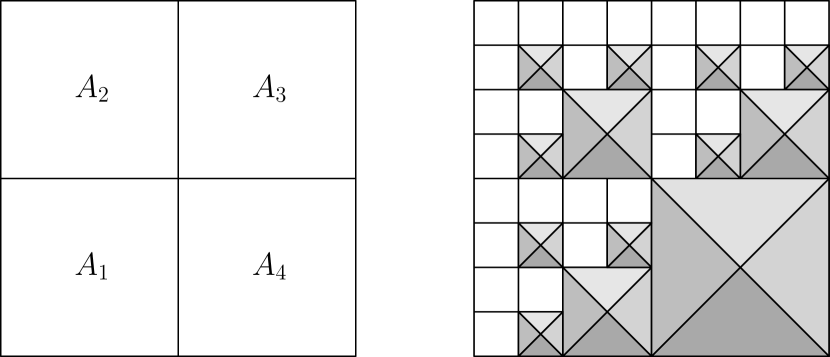
Figure 1: The plot on the left shows the square partition $\mathcal{P}$ which is repeated in a recursive manner. The right figure shows the function as a 2-dimensional projection for $k=3$. Each such pyramidal structure has a height of half the length of its base square.

This counterexample applies to any $d\geqslant 2$ simply by constructing a function that equals the above constructed function $f$ applied to two of its input variables. Such a function has infinite Hardy-Krause variation arising from the Vitali variation in those two variables. As a result, even if $f$ is in Lipschitz and $\tau$ is BVHK along with every component, we might still have $f\circ\tau\not\in{\mathrm{BVHK}}$.

3.2 Faa di Bruno formulas

We will study variation via a mixed partial derivative of the composition of the integrand on ${\mathcal{X}}$ with a transformation from the unit cube to ${\mathcal{X}}$. We need partial derivatives of order up to the dimension of the unit cube. High order derivatives of a composition become awkward even in the case with $d=m=1$, which was solved by Faa di Bruno, (1855). We will use a multivariable Faa di Bruno formula from Constantine and Savits, (1996).

To remain consistent with the notation in Constantine and Savits, (1996) we will consider functions $h=f(g(\cdot))$ here. After obtaining the formulas we need, we will revert to $f(\tau(\cdot))$ that is more suitable for the MC and QMC context.

To illustrate Faa di Bruno suppose first that $d=m=1$. Then let $g$ be defined on an open set containing $x_{0}$ and have derivatives up to order $n$ at $x_{0}$. Let $f$ be defined on an open set containing $y_{0}=g(x_{0})$ and have derivatives up to order $n$ at $y_{0}$. For $0\leqslant k\leqslant n$ define derivatives $f_{k}=\mathrm{d}^{k}f(y_{0})/\mathrm{d}y^{k}$, $g_{k}=\mathrm{d}^{k}g(x_{0})/\mathrm{d}x^{k}$ and $h_{k}=\mathrm{d}^{k}h(x_{0})/\mathrm{d}x^{k}$. From the chain rule we can easily find that

$$h_{4}=f_{4}g_{1}^{4}+6f_{3}g_{1}^{2}g_{2}+3f_{2}g_{2}^{2}+4f_{2}g_{1}g_{3}+f_{1}g_{4}.$$ (5)

The derivative $f_{k}$ appears in $h_{n}$ in as many terms as there are distinct ways of finding $k$ positive integers that sum to $n$. That number of terms is known as the Stirling number of the second kind (Graham et al.,, 1989). These Stirling numbers sum to the $n$’th Bell number which grows rapidly with $n$. We omit the $m=d=1$ Faa di Bruno formula for arbitrary $n$ and present instead the generalization due to Constantine and Savits, (1996).

In the multivariate setting, $h(\boldsymbol{x})=f({\boldsymbol{g}}(\boldsymbol{x}))$ where $\boldsymbol{x}\in{}^{m}$ and $\boldsymbol{y}={\boldsymbol{g}}(\boldsymbol{x})\in{}^{d}.$ In our applications $\boldsymbol{x}\in[0,1]^{m}$. We write ${\boldsymbol{g}}(\boldsymbol{x})=(g^{(1)}(\boldsymbol{x}),\dots,g^{(d)}(\boldsymbol{x}))$. The multivariate Faa di Bruno formula gives an arbitrary mixed partial derivative of $h$ with respect to components of $\boldsymbol{x}$ in terms of partial derivatives of $f$ and $g^{(i)}$. The formula requires that the needed derivatives exist.

The formula uses some multi-index notation. We use $\mathbb{N}_{0}$ for the set of non-negative integers. Let ${\boldsymbol{\nu}}=(\nu_{1},\dots,\nu_{m})\in\mathbb{N}_{0}^{m}$. Then $h_{\boldsymbol{\nu}}$ is the derivative of $h$ taken $\nu_{i}$ times with respect to $x_{i}$. Similarly $f$ and $g^{(i)}$ subscripted by tuples of $d$ and $m$ nonnegative integers respectively, are the corresponding partial derivatives. When the subscript is all zeros, the result is the function itself, undifferentiated.

For a multi-index ${\boldsymbol{\nu}}\in\mathbb{N}_{0}^{m}$ we write $|{\boldsymbol{\nu}}|=\sum_{i=1}^{m}\nu_{i}$ and ${\boldsymbol{\nu}}!=\prod_{i=1}^{m}(\nu_{i}!)$. For $\boldsymbol{z}\in{}^{m}$ and ${\boldsymbol{\nu}}\in\mathbb{N}_{0}^{m}$ we write $\boldsymbol{z}^{\boldsymbol{\nu}}$ for $\prod_{i=1}^{m}z_{i}^{\nu_{i}}$. We use an ordering $\prec$ on $\mathbb{N}_{0}^{m}$ where ${\boldsymbol{\mu}}\prec{\boldsymbol{\nu}}$ means that either $|{\boldsymbol{\mu}}|<|{\boldsymbol{\nu}}|$, or $|{\boldsymbol{\mu}}|=|{\boldsymbol{\nu}}|$ holds along with $\mu_{i}<\nu_{i}$ at the smallest $i$ where $\mu_{i}\neq\nu_{i}$. Multi-indices in $\mathbb{N}_{0}^{d}$ are treated the same way. The quantity ${\boldsymbol{g}}_{{\boldsymbol{\ell}}}$ is the vector $(g^{(1)}_{\boldsymbol{\ell}},\dots,g^{(d)}_{\boldsymbol{\ell}})$.

Theorem 1.

Let $g^{(i)}_{\boldsymbol{\mu}}$ be continuous in a neighborhood of $\boldsymbol{x}_{0}\in{}^{m}$ for all $|{\boldsymbol{\mu}}|\leqslant|{\boldsymbol{\nu}}|$ and all $i=1,\dots,d$, where ${\boldsymbol{\mu}},{\boldsymbol{\nu}}\in\mathbb{N}_{0}^{m}-\{{\boldsymbol{0}}\}$. Similarly, let $f_{\boldsymbol{\lambda}}$ be continuous in a neighborhood of $\boldsymbol{y}_{0}={\boldsymbol{g}}(\boldsymbol{x}_{0})$ for all $|{\boldsymbol{\lambda}}|\leqslant|{\boldsymbol{\nu}}|$. Then in a neighborhood of $\boldsymbol{x}_{0}$,

$$h_{\boldsymbol{\nu}} ={\boldsymbol{\nu}}!\sum_{1\leqslant|{\boldsymbol{\lambda}}|\leqslant|{\boldsymbol{\nu}}|}f_{\boldsymbol{\lambda}}\sum_{s=1}^{|{\boldsymbol{\nu}}|}\sum_{{\mathrm{KL}}(s,{\boldsymbol{\nu}},{\boldsymbol{\lambda}})}\prod_{r=1}^{s}\frac{[{\boldsymbol{g}}_{{\boldsymbol{\ell}}_{r}}]^{{\boldsymbol{k}}_{r}}}{({\boldsymbol{k}}_{r}!)[{\boldsymbol{\ell}}_{r}!]^{|{\boldsymbol{k}}_{r}|}},$$ (6)

where

$$\begin{split}{\mathrm{KL}}(s,{\boldsymbol{\nu}},{\boldsymbol{\lambda}})&=\Bigl{\{}({\boldsymbol{k}}_{1},\dots,{\boldsymbol{k}}_{s},{\boldsymbol{\ell}}_{1},\dots,{\boldsymbol{\ell}}_{s})\in\bigl{(}\mathbb{N}_{0}^{d}-\{{\boldsymbol{0}}\}\bigr{)}^{s}\times\bigl{(}\mathbb{N}_{0}^{m}-\{{\boldsymbol{0}}\}\bigr{)}^{s}\mid\\ &\qquad{\boldsymbol{\ell}}_{1}\prec{\boldsymbol{\ell}}_{2}\prec\dots\prec{\boldsymbol{\ell}}_{s},\ \sum_{r=1}^{s}{\boldsymbol{k}}_{r}={\boldsymbol{\lambda}},\ \text{and}\ \sum_{r=1}^{s}|{\boldsymbol{k}}_{r}|{\boldsymbol{\ell}}_{r}={\boldsymbol{\nu}}\Bigr{\}},\end{split}$$ (7)

Proof.

Constantine and Savits, (1996, Theorem 1). ∎

For our purposes of comparing geometric nets to (R)QMC, we only need $h_{\boldsymbol{\nu}}$ with ${\boldsymbol{\nu}}\in\{0,1\}^{m}-\{{\boldsymbol{0}}\}$. Equations (6) and (7) simplify.

Lemma 2.

For $m\geqslant 1$ let ${\boldsymbol{\nu}}\in\{0,1\}^{m}-\{{\boldsymbol{0}}\}$. If $1\leqslant|{\boldsymbol{\lambda}}|\leqslant|{\boldsymbol{\nu}}|$ and $1\leqslant s\leqslant|{\boldsymbol{\nu}}|$ and $({\boldsymbol{k}}_{1},\dots,{\boldsymbol{k}}_{s},{\boldsymbol{\ell}}_{1},\dots,{\boldsymbol{\ell}}_{s})\in{\mathrm{KL}}={\mathrm{KL}}(s,{\boldsymbol{\nu}},{\boldsymbol{\lambda}})$, then for $r=1,\dots,s$, ${\boldsymbol{k}}_{r}\in\{0,1\}^{d}-\{{\boldsymbol{0}}\}$, ${\boldsymbol{\ell}}_{r}\in\{0,1\}^{m}-\{{\boldsymbol{0}}\}$ and $|{\boldsymbol{k}}_{r}|=1$. Also ${\boldsymbol{\nu}}!={\boldsymbol{k}}_{r}!={\boldsymbol{\ell}}_{r}!=1$.

Proof.

Definition (7) of ${\mathrm{KL}}$ includes the condition $\sum_{r=1}^{s}|{\boldsymbol{k}}_{r}|{\boldsymbol{\ell}}_{r}={\boldsymbol{\nu}}$. Because ${\boldsymbol{\nu}}$ is a binary vector and $|{\boldsymbol{k}}_{r}|\geqslant 1$, no component of ${\boldsymbol{\ell}}_{r}$ can be larger than $1$. Therefore ${\boldsymbol{\ell}}_{r}\in\{0,1\}^{m}-\{{\boldsymbol{0}}\}$. Similarly ${\boldsymbol{\ell}}_{r}$ has at least one nonzero component and so $|{\boldsymbol{k}}_{r}|\leqslant 1$. Because ${\boldsymbol{k}}_{r}\neq{\boldsymbol{0}}$ we now have $|{\boldsymbol{k}}_{r}|=1$. Finally, the factorial of any binary vector is $1$. ∎

It follows from Lemma 2 that for ${\boldsymbol{\nu}}\in\{0,1\}^{m}-\{{\boldsymbol{0}}\}$,

$$h_{\boldsymbol{\nu}} =\sum_{1\leqslant|{\boldsymbol{\lambda}}|\leqslant|{\boldsymbol{\nu}}|}f_{\boldsymbol{\lambda}}\sum_{s=1}^{|{\boldsymbol{\nu}}|}\sum_{{\mathrm{KL}}(s,{\boldsymbol{\nu}},{\boldsymbol{\lambda}})}\prod_{r=1}^{s}[{\boldsymbol{g}}_{{\boldsymbol{\ell}}_{r}}]^{{\boldsymbol{k}}_{r}}.$$ (8)

Next, we use Lemma 2 to simplify the derivatives of $g$. Because ${\boldsymbol{\nu}}$ is a nonzero binary vector, we can identify it with a nonempty subset $v$ of $1{:}m$. Specifically, $j\in v$ if and only if $\nu_{j}=1$. Similarly we may identify the binary vector ${\boldsymbol{\ell}}_{r}\in\{0,1\}^{m}-\{{\boldsymbol{0}}\}$ with the set $\ell_{r}\subseteq 1{:}m$. The nonzero binary vector ${\boldsymbol{k}}_{r}\in\{0,1\}^{d}$ corresponds to a singleton set. We can therefore identify it with an integer in $1{:}d$. We identify ${\boldsymbol{k}}_{r}$ with the integer $k_{r}$ such that ${\boldsymbol{k}}_{ri}=1$ if and only if $i=k_{r}$.

With this identification,

$$[{\boldsymbol{g}}_{{\boldsymbol{\ell}}_{r}}]^{{\boldsymbol{k}}_{r}}=\prod_{i=1}^{d}\biggl{(}\frac{\partial^{|{\boldsymbol{\ell}}_{r}|}g^{(i)}}{\prod_{r=1}^{s}\partial x_{r}^{\ell_{jr}}}\biggr{)}^{k_{ri}}=\prod_{i=1}^{d}\bigl{(}\partial^{\ell_{r}}g^{(i)}\bigr{)}^{k_{ri}}=\partial^{\ell_{r}}g^{(k_{r})}.$$ (9)

Now switching from $g^{(k)}$ back to $\tau_{k}$ we get a Faa di Bruno formula for mixed partial derivatives taken at most once with respect to every index:

$$\partial^{v}(f\circ\tau) =\sum_{{\boldsymbol{\lambda}}\in\mathbb{N}_{0}^{m}\atop 1\leqslant|{\boldsymbol{\lambda}}|\leqslant|v|}f_{\boldsymbol{\lambda}}\sum_{s=1}^{|v|}\sum_{(\ell_{r},k_{r})\in{{\widetilde{\mathrm{KL}}}}(s,v,{\boldsymbol{\lambda}})}\prod_{r=1}^{s}\partial^{\ell_{r}}\tau_{k_{r}}$$ (10)

where ${\widetilde{\mathrm{KL}}}(s,v,{\boldsymbol{\lambda}})$ equals

$$\begin{split}&\Bigl{\{}(\ell_{r},k_{r}),\ r=1,\dots,s,\ \Bigm{|}\ell_{r}\subseteq 1{:}m,\ k_{r}\in 1{:}d,\ \cup_{r=1}^{s}\ell_{r}=v,\\ &\qquad\ell_{r}\cap\ell_{r^{\prime}}=\varnothing\ \text{for}\ r\neq r^{\prime}\ \text{and}\ |\{j\in 1{:}s\mid k_{j}=i\}|=\lambda_{i}\Bigr{\}}.\end{split}$$ (11)

4 Necessary and sufficient conditions

Equation (10) allows us to find sufficient conditions on $f$ and $\tau$ so that $f\circ\tau\in{\mathrm{BVHK}}$. Uniformity transformations $\tau$ satisfy (1). We don’t need that condition for $f\circ\tau\in{\mathrm{BVHK}}$ but we do need it to ensure that averages of $f\circ\tau$ over $[0,1]^{m}$ estimate ${\mathbf{vol}}({\mathcal{X}})^{-1}\int_{{\mathcal{X}}}f(\boldsymbol{x})\mathrm{\,d}\boldsymbol{x}$. We find conditions on $\tau$ so that $f\circ\tau\in{\mathrm{BVHK}}$ for all $f\in C^{m}({\mathcal{X}})$. Similarly we find conditions under which $f\circ\tau$ is smooth in the sense of equation (4) for all $f\in C^{m}({\mathcal{X}})$.

We will use a generalized Hölder inequality (Bogachev,, 2007, page 141). For a positive integer $s$ suppose that $f_{r}\in L^{p_{r}}(\mu)$ for $r=1,\dots,s$, for some nonnegative measure $\mu$, and that $\sum_{r=1}^{s}1/p_{r}=1/p$. Then $(\int|\prod_{r=1}^{s}f_{r}|^{p}\mathrm{\,d}\mu)^{1/p}\leqslant\prod_{r=1}^{s}(\int|f_{r}|^{p_{r}}\mathrm{\,d}\mu)^{1/p_{r}}$ and so $\prod_{r=1}^{s}f_{r}\in L^{p}(\mu)$.

Theorem 2.

Let $\tau(\boldsymbol{u})=(\tau_{1}(\boldsymbol{u}),\ldots,\tau_{d}(\boldsymbol{u}))$ be a map from $[0,1]^{m}$ to the closed and bounded set ${\mathcal{X}}\subset{}^{d}$ such that $\partial^{1:m}\tau_{j}$ exists for all $j=1,\dots,d$. Assume that $\partial^{v}\tau_{j}(\boldsymbol{u}_{v}{:}{\boldsymbol{1}}_{-v})\in L^{p_{j}}\bigl{(}[0,1]^{|v|}\bigr{)}$ for all $j=1,\ldots,d$ and for all nonempty $v\subseteq 1{:}m$, where $p_{j}\in[1,\infty]$. If $\sum_{j=1}^{d}1/p_{j}\leqslant 1$ then $f\circ\tau\in{\mathrm{BVHK}}$ for all $f\in C^{d}({\mathcal{X}})$.

Proof.

From (3) we need to show that $\partial^{v}(f\circ\tau)(\boldsymbol{u}_{v}{:}{\boldsymbol{1}}_{-v})\in L_{1}[0,1]^{|v|}$ for nonempty $v\subseteq 1{:}m$. From (10) it suffices to show that

$$\int_{[0,1]^{|v|}}\Bigl{|}f_{{\boldsymbol{\lambda}}}(\tau(\boldsymbol{u}_{v}{:}{\boldsymbol{1}}_{-v}))\prod_{r=1}^{s}\partial^{\ell_{r}}\tau_{k_{r}}(\boldsymbol{x}_{u}{:}{\boldsymbol{1}}_{-u})\Bigr{|}\mathrm{\,d}\boldsymbol{x}_{u}<\infty$$ (12)

for all ${\boldsymbol{\lambda}}\in\mathbb{N}_{0}^{d}$ with $1\leqslant|{\boldsymbol{\lambda}}|\leqslant|v|$, all $s\leqslant|v|$, all disjoint $\ell_{r}\subseteq v$ with union $v$, where $\lambda_{i}$ of the $k_{r}$ are equal to $i$ for $i\in 1{:}d$. Because $f_{\boldsymbol{\lambda}}$ is uniformly bounded the integral in (12) can be bounded by a product of univariable integrals. The result then follows from our assumptions and from the generalized Hölder inequality. ∎

As a special case, consider $p_{j}=d$ for $j=1,\dots,d$. Notice that the moment conditions on $\tau$ become more stringent as the dimension $d$ of ${\mathcal{X}}$ increases. Attaining the usual QMC rate becomes increasingly difficult in higher dimensions for QMC applied through a transformation $\tau$.

Next we consider the kind of smoothness that allows scrambled nets to improve upon the quasi-Monte Carlo rate. In this setting we require mixed partial derivatives in $L^{2}$ but we do not have to pay special attention to components of $\boldsymbol{u}$ that equal $1$.

Theorem 3.

Let $\tau(\boldsymbol{u})=(\tau_{1}(\boldsymbol{u}),\ldots,\tau_{d}(\boldsymbol{u}))$ be a map from $[0,1]^{m}$ to the closed and bounded set ${\mathcal{X}}\subset{}^{d}$ such that $\partial^{1:m}\tau_{j}$ exists for all $j=1,\dots,d$. Assume that $\partial^{v}\tau_{j}\in L^{p_{j}}([0,1]^{m})$ for all $j=1,\ldots,d$ and for all nonempty $v\subseteq 1{:}m$, where $p_{j}\in[1,\infty]$. If $\sum_{j=1}^{d}1/p_{j}\leqslant 1/2$, then $f\circ\tau$ is smooth in the sense of equation (4) for all $f\in C^{d}({\mathcal{X}})$.

Proof.

Essentially the same argument that proves Theorem 2 applies here. ∎

Necessary conditions are more subtle. To take an extreme case, $\tau$ could fail to be in ${\mathrm{BVHK}}$ or to be smooth, but $f$ could repair that problem by being constant everywhere, or just in a region outside of which $\tau$ is well behaved. Our working definition is that we consider a transformation $\tau$ to be unsuitable for QMC when one or more of the components $\tau_{j}$ has $\partial^{u}\tau_{j}(\cdot:1_{-v})\not\in L_{1}$ for some $v\subset 1{:}m$. In that case even the coordinate function $\tau_{j}\not\in{\mathrm{BVHK}}$. Similarly if $\partial^{v}\tau_{j}\not\in L^{2}$ for any $j$ and $v$ then the transformation $\tau$ is one that does not lead to the improved rate for scrambled nets even for integration of $\tau$, much less $f\circ\tau$ for all $f\in C^{d}({\mathcal{X}})$.

It is possible to weaken the condition on $f$ in Theorem 2, while strengthening the conditions on $\tau_{j}$. We could require only that $(f_{\boldsymbol{\lambda}}\circ\tau)(\cdot{:}{\boldsymbol{1}}_{-v})$ is in $L^{p_{0}}([0,1]^{|v|})$ whenever $|{\boldsymbol{\lambda}}|\leqslant m$ and then require $\sum_{j=0}^{d}1/p_{j}\leqslant 1$. Similarly for Theorem 3, we could require $f_{\boldsymbol{\lambda}}\circ\tau\in L^{p_{0}}$ whenever $|{\boldsymbol{\lambda}}|\leqslant m$ where $\sum_{j=0}^{d}1/p_{j}\leqslant 1/2$.

5 Counter-Examples

In this section we give two common transformations for which some $\tau_{j}\not\in{\mathrm{BVHK}}$, which means we do not satisfy the conditions of Theorem 2. Thus unless we are very lucky, we would have ${\mathrm{V}_{\mathrm{HK}}}(f\circ\tau)=\infty$.

5.1 Map from $[0,1]^{3}$ to an equilateral triangle

Let $T^{2}=\{\boldsymbol{x}\in[0,1]^{3}\mid\sum_{j=1}^{3}x_{j}=1\}$, an equilateral triangle. Consider the map $\tau:[0,1]^{3}\rightarrow T^{2}$ defined by

$$\tau_{j}(\boldsymbol{u})=\frac{\log u_{j}}{\sum_{i=1}^{3}\log u_{i}},\quad j=1,2,3.$$ (13)

It is well known that $\tau(\boldsymbol{u})\sim\mathbf{U}(T^{2})$ when $\boldsymbol{u}\sim\mathbf{U}([0,1]^{3})$. The mapping in (13) is well defined for $\boldsymbol{u}\in(0,1)^{3}$. There are various reasonable ways to extend it to problematic boundary points with either some $u_{j}=0$ or with all $u_{j}=1$. We will show that none of those extensions can yield $\tau_{j}\in{\mathrm{BVHK}}$.

First we find that

$$\begin{split}\iint_{(0,1)^{2}}\left|\frac{\partial^{2}\tau_{1}}{\partial u_{1}\partial u_{2}}\right|_{u_{3}=1}\mathrm{\,d}u_{1}\mathrm{\,d}u_{2}&=\iint_{(0,1)^{2}}\left|\frac{\log u_{1}-\log u_{2}}{u_{1}u_{2}(\sum_{i=1}^{2}\log u_{i})^{3}}\right|\mathrm{\,d}u_{1}\mathrm{\,d}u_{2}.\end{split}$$

After a change of variable to $x_{1}=\log u_{1}$ and $x_{2}=\log u_{2}$ the integral becomes

$$\begin{split}&\int_{-\infty}^{0}\int_{-\infty}^{0}\left|\frac{x_{1}-x_{2}}{(x_{1}+x_{2})^{3}}\right|\mathrm{\,d}x_{1}\mathrm{\,d}x_{2}\\ &=\int_{-\infty}^{0}\int_{-\infty}^{x_{1}}\frac{x_{1}-x_{2}}{(x_{1}+x_{2})^{3}}\mathrm{\,d}x_{2}\mathrm{\,d}x_{1}+\int_{-\infty}^{0}\int_{x_{1}}^{0}\frac{x_{2}-x_{1}}{(x_{1}+x_{2})^{3}}\mathrm{\,d}x_{2}\mathrm{\,d}x_{1}\\ &=\int_{-\infty}^{0}\frac{1}{2x_{1}}dx_{1}=\infty.\end{split}$$

Thus $\tau\not\in{\mathrm{BVHK}}$. There is no extension from $(0,1)^{3}$ to $[0,1]^{3}$ that would yield $\tau\in{\mathrm{BVHK}}$. The same argument applies if $\tau_{j}(\boldsymbol{u})=\log(u_{j})/\sum_{i=1}^{m}\log(u_{i})$ for any $m\geqslant 3$, mapping $[0,1]^{m}$ to a $d=m-1$ dimensional simplex. We can set $u_{i}=1$ for $i\geqslant 3$ and integrate as before.

5.2 Inverse Gaussian map to the hypersphere

A very convenient way to sample uniformly from the sphere $\mathbb{S}^{d-1}=\{\boldsymbol{x}\in{}^{d}\mid\|\boldsymbol{x}\|=1\}$ is to generate $d$ independent $\mathcal{N}(0,1)$ random variables and standardize them. We write $\varphi$ and $\Phi$ for the probability density function and cumulative distribution function, respectively, of $\mathcal{N}(0,1)$. The mapping from $[0,1]^{d}$ to ${\mathcal{X}}=\mathbb{S}^{d-1}$ is

$$\tau_{j}(\boldsymbol{u})=\frac{\Phi^{-1}(u_{j})}{\sqrt{\sum_{i=1}^{d}\Phi^{-1}(u_{i})^{2}}}.$$

We will use the double factorial function $n!!=n(n-2)(n-4)\cdots 1$ for odd $n$ and set $g(n)=(2n-1)!!$. For $j\in 1{:}d$ and $v\subset 1{:}d$ with $j\not\in v$ we find that

$$\partial^{v}\tau_{j}=\frac{(-1)^{|v|}g(|v|)\Phi^{-1}(u_{j})}{\bigl{(}\sum_{i=1}^{d}\Phi^{-1}(u_{i})^{2}\bigr{)}^{|v|+1/2}}\times\prod_{i\in v}\frac{\Phi^{-1}(u_{i})}{\varphi(\Phi^{-1}(u_{i}))}.$$

Now if $j\in v$, we can write after some algebra,

$$\partial^{v}\tau_{j} =\frac{\partial}{\partial u_{j}}\partial^{v-\{j\}}\tau_{j}$$

$$=\frac{(-1)^{|v|}g(|v|)\prod_{i\in v-\{j\}}\Phi^{-1}(u_{i})\bigl{[}2(|v|-1)\Phi^{-1}(u_{j})^{2}-\sum_{i\neq j}\Phi^{-1}(u_{i})^{2}\bigr{]}}{\bigl{(}\sum_{i=1}^{d}\Phi^{-1}(u_{i})^{2}\bigr{)}^{|v|+1/2}\prod_{i\in v}\phi(\Phi^{-1}(u_{i}))}.$$

We choose $v=1{:}d$ and integrate $|\partial^{1{:}d}\tau_{j}|$ over $[0,1]^{d}$. The integration is done with a change of variable $x_{i}=\Phi^{-1}(u_{i})$ so $\mathrm{\,d}u_{i}=\varphi(x_{i})\mathrm{\,d}x_{i}$. Because $g(d-1)\geqslant 1$,

$$\begin{split}\int_{[0,1]^{d}}\bigl{|}\partial^{1:d}\tau_{j}\bigr{|}\mathrm{\,d}u&\geqslant\int_{{}^{d}}\Biggl{|}\frac{\prod_{i\neq j}x_{i}\bigl{[}2(d-1)x_{j}^{2}-\sum_{i\neq j}x_{i}^{2}\bigr{]}}{\bigl{(}\sum_{i=1}^{d}x_{i}^{2}\bigr{)}^{d+1/2}}\Biggr{|}\mathrm{\,d}\boldsymbol{x}\\ &\geqslant\int_{[0,\infty)^{d-1}}\int_{0}^{\infty}\frac{\left|\prod_{i\neq j}x_{i}\bigl{[}2(d-1)x_{j}^{2}-\sum_{i\neq j}x_{i}^{2}\bigr{]}\right|}{\bigl{(}\sum_{i=1}^{d}x_{i}^{2}\bigr{)}^{d+1/2}}\mathrm{\,d}x_{j}\mathrm{\,d}\boldsymbol{x}_{-j}\\ &\geqslant\int_{[0,\infty)^{d-1}}\int_{0}^{\bigl{(}\frac{\sum_{i\neq j}x_{i}^{2}}{2(d-1)}\bigr{)}^{1/2}}\frac{\prod_{i\neq j}x_{i}\bigl{[}\sum_{i\neq j}x_{i}^{2}-2(d-1)x_{j}^{2}\bigr{]}}{\bigl{(}\sum_{i=1}^{d}x_{i}^{2}\bigr{)}^{d+1/2}}\mathrm{\,d}x_{j}\mathrm{\,d}\boldsymbol{x}_{-j}\\ &\geqslant\int_{[0,\infty)^{d-1}}\prod_{i\neq j}x_{i}\int_{0}^{\bigl{(}\frac{\sum_{i\neq j}x_{i}^{2}}{2(d-1)}\bigr{)}^{1/2}}\frac{\bigl{[}\sum_{i\neq j}x_{i}^{2}-2(d-1)x_{j}^{2}\bigr{]}}{\bigl{(}\frac{2d-1}{2d-2}\sum_{i\neq j}^{d}x_{i}^{2}\bigr{)}^{d+1/2}}\mathrm{\,d}x_{j}\mathrm{\,d}\boldsymbol{x}_{-j}\\ &=\tilde{K}\int_{[0,\infty)^{d-1}}\frac{\prod_{i\neq j}x_{i}}{\bigl{(}\sum_{i\neq j}x_{i}^{2}\bigr{)}^{d-1}}\mathrm{\,d}\boldsymbol{x}_{-j}\end{split}$$

where $\tilde{K}=((2d-2)/(2d-1))^{d+1/2}$.

Now we integrate this one at a time for each $i\neq j$. Note that for $k<d-1$,

$$\int_{0}^{\infty}\frac{x}{(x^{2}+z)^{d-k}}dx=c_{k}\frac{1}{z^{d-k-1}}$$ (14)

where $c_{k}=1/(2(d-k-1))$. Applying (14) repeatedly for $k=1$ to $k=d-2$, we get

$$\begin{split}\int_{[0,1]^{d}}\left|\partial^{1:d}\tau_{j}\right|\mathrm{\,d}\boldsymbol{u}&\geqslant\left(\tilde{K}\prod_{k=1}^{d-2}c_{k}\right)\int_{0}^{\infty}\frac{1}{x_{j}}\mathrm{\,d}x_{j}=\infty\end{split}$$

and so $\tau_{j}\not\in{\mathrm{BVHK}}$ for all $j\in 1{:}d$.

6 Mappings from Fang and Wang, (1993)

Fang and Wang, (1993) provide mappings from the unit cube to other important spaces for quadrature problems. Their mappings are more complicated than the elegant symmetric ones in Section 5. Instead of symmetry, their mappings are designed to use a unit cube of exactly the same dimension as the space they map too. The domains that they consider, and their nomenclature for them, are:

$$\begin{split}A_{d}&=\{(x_{1},\ldots,x_{d}):0\leqslant x_{1}\leqslant\ldots\leqslant x_{d}\leqslant 1\}\\ B_{d}&=\{(x_{1},\ldots,x_{d}):x_{1}^{2}+\ldots+x_{d}^{2}\leqslant 1\}\\ U_{d}&=\{(x_{1},\ldots,x_{d}):x_{1}^{2}+\ldots+x_{d}^{2}=1\}\\ V_{d}&=\{(x_{1},\ldots,x_{d})\in\mathbb{R}_{+}^{d}:x_{1}+\ldots+x_{d}\leqslant 1\},\quad\text{and}\\ T_{d}&=\{(x_{1},\ldots,x_{d})\in\mathbb{R}_{+}^{d}:x_{1}+\ldots+x_{d}=1\}.\end{split}$$ (15)

Spaces $A_{d}$, $V_{d}$ and $T_{d+1}$ are all simplices of dimension $d$, $B_{d}$ is a ball and $U_{d}$ is the $d-1$ dimensional hyper-sphere.

We show next that all of their mappings have components $\tau$ in BVHK and none of them have all mixed partial derivatives in $L^{2}$. They are thus better suited to QMC than the symmetric mappings are but they are not able to take advantage of the improved rate for RQMC versus QMC. The transformations have a separable character that lets us study them directly without recourse to the generalized Hölder inequality.

6.1 Mapping from $[0,1]^{d}$ to $A_{d}$

The map $\tau=(\tau_{1},\ldots,\tau_{d})$ is given by $\tau_{j}(\boldsymbol{u})=\prod_{i=j}^{d}u_{i}^{1/i}$ for $j=1,\ldots,d$. We find that

$$(\partial^{1:d}\tau_{1})^{2}=\prod_{i=1}^{d}\frac{1}{i^{2}}u_{i}^{2/i-2}$$

which diverges on integrating with respect to $u_{2}$. Thus $\partial^{1{:}d}\tau_{1}$ is not in $L^{2}$, outside the trivial case $d=1$.

Next, we show that $\tau_{j}$ is in BVHK. Pick any non-empty $v\subseteq 1{:}d$. If there exists $i\in v$ with $i<j$, then $\partial^{v}\tau_{j}=0$, so we may assume that $v\subseteq j{:}d$. For such a $v$, we have,

$$\int_{[0,1]^{|v|}}|\partial^{v}\tau_{j}(\boldsymbol{u}_{v}{:}{\boldsymbol{1}}_{-u})|\mathrm{\,d}\boldsymbol{u}_{v}=\int_{[0,1]^{|v|}}\biggl{|}\prod_{i\in v}\frac{1}{i}u_{i}^{1/i-1}\biggr{|}\mathrm{\,d}\boldsymbol{u}_{v}=1.$$

Thus, using (3) we find that $\tau_{j}$ are BVHK for all $j$.

6.2 Mapping from $[0,1]^{d}$ to $B_{d}$

The mapping involves the inverse transform of a distribution function on $B_{d}$. Define,

$$F_{j}(x)=\begin{cases}x^{d},&\mbox{if }j=1\\ \frac{\pi}{B\left(\frac{1}{2},\frac{d-j+1}{2}\right)}\int_{0}^{x}(\sin\pi t)^{d-j}\mathrm{\,d}t,&\mbox{if }j=2,\ldots,d\end{cases}$$

where $B(\cdot,\cdot)$ is the Beta function. Next define intermediate variables

$$b_{1} =u_{1}^{1/d}\quad\text{and}\quad b_{i}=F_{i}^{-1}(u_{i}),\qquad\text{for }i=2,\ldots,d.$$

Their mappings are then

$$\tau_{j} =b_{1}\prod_{i=2}^{j}\sin(\pi b_{i})\cos(\pi b_{j+1}),\quad\text{for }1\leqslant j\leqslant d-2,$$

$$\tau_{d-1} =b_{1}\prod_{i=2}^{d-1}\sin(\pi b_{i})\cos(2\pi b_{d}),\quad\text{and}$$

$$\tau_{d} =b_{1}\prod_{i=2}^{d-1}\sin(\pi b_{i})\sin(2\pi b_{d}).$$

For $d=2$ we get $F_{2}(x)=x$ and so $\tau_{2}=u_{1}^{1/2}\sin(2\pi u_{2})$. Therefore $\partial^{1:2}\tau_{2}={\pi\cos(2\pi u_{2})}/{\sqrt{u_{1}}}$ which is not in $L^{2}$. For general $d>2$, we have,

$$\partial^{1:d}\tau_{d}=\frac{1}{d}u_{1}^{1/d-1}\left(\prod_{i=2}^{d-1}\pi\cos(\pi b_{i})\frac{\partial b_{i}}{\partial u_{i}}\right)2\pi\cos(2\pi u_{d}),$$ (16)

which is also not in $L^{2}$ because of the factor $u_{1}^{1/d-1}$.

For later use with the transformation to $U_{d}$, we also consider the factor for $i=d-1$ in (16). The definition of $b_{d-1}$ simplifies to $b_{d-1}=\cos^{-1}(1-2u_{d-1})/\pi$ and so

$$\frac{\partial b_{d-1}}{\partial u_{d-1}}=\frac{2}{\pi\sin(\pi b_{d-1})}.$$

This simplifies the above mixed partial to

$$\partial^{1:d}\tau_{d}=\frac{1}{d}u_{1}^{1/d-1}\left(\prod_{i=2}^{d-2}\pi\cos(\pi b_{i})\frac{\partial b_{i}}{\partial u_{i}}\right)\left(2\frac{(1-2u_{d-1})}{\sqrt{1-(1-2u_{d-1})^{2}}}\right)2\pi\cos(2\pi u_{d})$$

Now

$$\int_{0}^{1}\frac{(1-2u_{d-1})^{2}}{1-(1-2u_{d-1})^{2}}du_{d-1}=\frac{1}{4}\left(\log x-\log(1-x)-4x\right)\Bigg{|}_{0}^{1}=\infty.$$ (17)

To show that this transformation is in BVHK we follow the proof of Theorem 2. Assuming $f\in C^{d}$, using (12) it is enough to show that

$$\int_{[0,1]^{|v|}}\Bigl{|}\prod_{r=1}^{s}\partial^{\ell_{r}}\tau_{k_{r}}(\boldsymbol{u}_{v}{:}{\boldsymbol{1}}_{-v})\Bigr{|}\mathrm{\,d}\boldsymbol{u}_{v}<\infty,$$

for $v\subseteq 1{:}m$, $s\leqslant|v|$ and $k_{r}\in 1{:}d$. Note that $\ell_{r}\cap\ell_{r^{\prime}}=\varnothing$ for all $r\neq r^{\prime}$ and $\cup_{r}\ell_{r}=v$. Thus, we differentiate at most once with respect to any original variable and we get,

$$\int_{[0,1]^{|v|}}\Bigl{|}\prod_{r=1}^{s}\partial^{\ell_{r}}\tau_{k_{r}}(\boldsymbol{u}_{v}{:}{\boldsymbol{1}}_{-v})\Bigr{|}\mathrm{\,d}\boldsymbol{u}_{v}\leqslant\int_{[0,1]^{|v|}}\Bigl{|}\prod_{i\in v}\frac{\partial b_{i}}{\partial u_{i}}\Bigr{|}\mathrm{\,d}\boldsymbol{u}_{v}\leqslant\prod_{i\in v}\int_{[0,1]}\Bigl{|}\frac{\partial b_{i}}{\partial u_{i}}\Bigr{|}\mathrm{\,d}u_{i}.$$

Now

$$\frac{\partial b_{i}}{\partial u_{i}}=\frac{B\left(\frac{1}{2},\frac{d-j+1}{2}\right)}{\pi\left[\sin\left(\pi F_{i}^{-1}(u_{i})\right)\right]^{d-i}}.$$

Note that $F_{i}^{-1}(u_{i})\in[0,1]$ for all $u_{i}\in[0,1]$. Thus we have,

$$\int_{[0,1]}\Bigl{|}\frac{\partial b_{i}}{\partial u_{i}}\Bigr{|}\mathrm{\,d}u_{i}=\int_{[0,1]}\frac{\partial b_{i}}{\partial u_{i}}\mathrm{\,d}u_{i}=1$$

which shows that $\tau$ is BVHK.

6.3 Mapping from $[0,1]^{d-1}$ to $U_{d}$

This mapping is similar to one in $B_{d}$, with the densities being different. Here we have,

$$f_{j}(u)=\frac{\pi}{B\left(\frac{1}{2},\frac{d-j}{2}\right)}(\sin(\pi u))^{d-j-1}$$

and $b_{i}=F_{i}^{-1}(u_{i})$ for $i=1,\ldots,d-1$. The explicit transformation can be written as

$$\tau_{j} =\prod_{i=1}^{j-1}\sin(\pi b_{i})\cos(\pi b_{j})\qquad\text{for }j=1,\ldots,d-2$$

$$\tau_{d-1} =\prod_{i=1}^{d-2}\sin(\pi b_{i})\cos(2\pi b_{d-1}),\quad\text{and}$$

$$\tau_{d} =\prod_{i=1}^{d-2}\sin(\pi b_{i})\sin(2\pi b_{d-1}).$$

We first consider the case $d=2$. It is easy to see that

$$\tau_{1}=\cos(2\pi u_{1})\quad\text{and}\quad\tau_{2}=\sin(2\pi u_{1}).$$

Note that in this case, $\partial^{v}\tau_{j}\in L^{2}$ for each $v\subseteq\{1,2\}$ and $j=1,2$. This is the only case with this property, but then the set $U_{d}$ is intrinsically one dimensional. For $d\geqslant 3$, consider the $(d-2)$-th term in the expansion of $\partial^{1:d-1}\tau_{d}$,

$$\partial^{1:d-1}\tau_{d}=\left(\prod_{i=1}^{d-3}\pi\cos(\pi bi)\frac{\partial b_{i}}{\partial u_{i}}\right)\left(2\frac{(1-2u_{d-2})}{\sqrt{1-(1-2u_{d-2})^{2}}}\right)2\pi\cos(2\pi u_{d-1}).$$

Using (16) as in the previous case, this proves that $\partial^{1:d-1}\tau_{d}\not\in L^{2}$. Furthermore, following the same argument in Section 6.2, we may show that this transformation is also in BVHK.

6.4 Mapping from $[0,1]^{d}$ to $V_{d}$

Here we have,

$$\tau_{i} =u_{1}^{1/d}\prod_{j=2}^{i}u_{j}^{\frac{1}{d-j+1}}\Bigl{(}1-u_{i+1}^{\frac{1}{d-i}}\Bigr{)}\qquad\text{for }i=1,\ldots,d-1,\quad\text{and}$$

$$\tau_{d} =u_{1}^{1/d}\prod_{j=2}^{d}u_{j}^{\frac{1}{d-j+1}}.$$

Considering the mixed partial, $\partial^{1:d}\tau_{d}$ we have

$$\partial^{1:d}\tau_{d} =\frac{1}{d}u_{1}^{\frac{1}{d}-1}\prod_{j=2}^{d}\frac{1}{d-j+1}u_{j}^{\frac{1}{d-j+1}-1}=\frac{1}{d!}\frac{1}{u_{1}^{\frac{d-1}{d}}u_{2}^{\frac{d-2}{d-1}}\ldots u_{d-1}^{1/2}}.$$

Observing the integral with respect to $u_{d-1}$ it is clear that $\partial^{1:d}\tau_{d}\not\in L^{2}$. Furthermore, following the same argument in Section 6.1, we may show that this transformation is also in BVHK.

6.5 Mapping from $[0,1]^{d-1}$ to $T_{d}$

Similar to $V_{d}$, here we have,

$$\tau_{i} =\prod_{j=1}^{i-1}u_{j}^{\frac{1}{d-j}}\Bigl{(}1-u_{i}^{\frac{1}{d-i}}\Bigr{)}\qquad\text{for }i=1,\ldots,d-1$$

$$\tau_{d} =\prod_{j=1}^{d-1}u_{j}^{\frac{1}{d-j}}.$$

It is thus clear from

$$\partial^{1:d-1}\tau_{d}=\frac{1}{(s-1)!}\frac{1}{u_{1}^{\frac{d-2}{d-1}}u_{2}^{\frac{d-3}{d-2}}\ldots u_{d-2}^{1/2}u_{d-1}}$$

that $\partial^{1:d-1}\tau_{d}\not\in L^{2}$. The argument from Section 6.1 shows that this transformation is in BVHK.

6.6 Efficient mapping from $[0,1]^{d-1}$ to $U_{d}$

Fang and Wang, (1993) gave another mapping to $U_{d}$ which avoids computing the incomplete beta function that was used in Section 6.3. Once again the transformation fails to have all partial derivatives in $L^{2}$. We deal with the case of $d$ being even and odd differently.

Even case: $d=2m$

Here we have $(u_{1},\ldots,u_{d-1})\in[0,1]^{d-1}$. Define $g_{m}=1$ and $g_{0}=0$. For $j$ from $m-1$ down to $1$, let $g_{j}=g_{j+1}u_{j}^{1/j}$. Put $d_{l}=\sqrt{g_{l}-g_{l-1}}$. Now for $l=1,\ldots,m$, define

$$\tau_{2l-1} =d_{l}\cos(2\pi u_{m+l-1})\quad\text{and}\quad\tau_{2l}=d_{l}\sin(2\pi u_{m+l-1}).$$

It is easy to see that

$$\tau_{1}=d_{1}\cos(2\pi u_{m})=\prod_{j=1}^{m-1}u_{j}^{1/2j}\cos(2\pi u_{m})$$

and so

$$|\partial^{1:m}\tau_{1}| =\Biggl{|}\prod_{j=1}^{m-1}\frac{1}{2j}u_{j}^{1/2j-1}2\pi\sin(2\pi u_{m})\Biggr{|}=\Biggl{|}\frac{1}{2^{m-1}(m-1)!}\frac{2\pi\sin(2\pi u_{m})}{u_{1}^{\frac{1}{2}}u_{2}^{\frac{3}{4}}\ldots u_{m-1}^{\frac{2m-3}{2m-2}}}\Biggr{|}.$$

Integrating with respect to $u_{1}$ shows that $\partial^{1:m}\tau_{1}\not\in L^{2}$.

Odd case: $d=2m+1$

Again we begin with $(u_{1},\ldots,u_{d-1})\in[0,1]^{d-1}$. Define $g_{m}=1$ and $g_{0}=0$. For $j=m-1$ down to $j=1$, let $g_{j}=g_{j+1}u_{j}^{{2}/(2j+1)}$. As for the even case, put $d_{l}=\sqrt{g_{l}-g_{l-1}}$. Now for $l=2,\ldots,m$, define

$$\tau_{1} =d_{1}(1-2u_{m}),$$

$$\tau_{2} =d_{1}\sqrt{u_{m}(1-u_{m})}\cos(2\pi u_{m+1}),$$

$$\tau_{3} =d_{1}\sqrt{u_{m}(1-u_{m})}\sin(2\pi u_{m+1}),\quad\text{and then}$$

$$\tau_{2l} =d_{l}\cos(2\pi u_{2l}),\quad\text{and}\quad\tau_{2l+1}=d_{l}\sin(2\pi u_{2l}).$$

Simplifying $d_{1}$ we see that

$$\tau_{2}=u_{1}^{\frac{1}{3}}u_{2}^{\frac{1}{5}}\ldots u_{m-1}^{\frac{1}{2m-1}}\sqrt{u_{m}(1-u_{m})}\cos(2\pi u_{m+1})$$

Thus

$$\left|\frac{\partial\tau_{2}}{\partial u_{m}}\right|_{u_{j}=1,j\neq m}=\frac{1-2u_{m}}{2\sqrt{u_{m}(1-u_{m})}}$$

Applying (17) we see that $\partial^{u_{m}}\tau_{2}\not\in L^{2}$.

All of the $\tau_{j}$ are in BVHK. This follows from the fact that each component of the transformation is a product of functions of only one of the original variables and hence it is completely separable.

7 Nonuniform transformations

Here we consider transformations that are not uniformity preserving. Section 7.1 considers importance sampling methods for integrals with respect to a non-uniform measure on ${\cal X}$. Section 7.2 gives conditions for sequential inversion to yield an integrand in BVHK. Section 7.3 shows that some importance sampling transformations lead to the $O(n^{-3/2+\epsilon})$ rate for RMSE on the simplex for a class of functions including polynomials.

Suppose that $\mu=\int_{{\cal X}}f(\boldsymbol{x})p(\boldsymbol{x})\mathrm{\,d}\boldsymbol{x}$ for a nonuniform density $p$. Instead of sampling drawing $\boldsymbol{x}_{i}$ from the uniform distribution on ${\cal X}$ and averaging $fp$, a Monte Carlo strategy can be to sample $\boldsymbol{x}_{i}\sim p$ and average $f$, or under conditions, sample $\boldsymbol{x}_{i}\sim q$ and average $fp/q$. This latter is importance sampling.

Aistleitner and Dick, (2015) show that if $f$ is a measurable function on $[0,1]^{d}$ which is BVHK and $P$ is a normalized Borel measure on $[0,1]^{d}$, then for $\boldsymbol{x}_{1},\ldots,\boldsymbol{x}_{n}$ in $[0,1]^{d}$,

$$\left|\frac{1}{n}\sum_{i=1}^{n}f(\boldsymbol{x}_{i})-\int_{[0,1]^{d}}f(\boldsymbol{x})\mathrm{\,d}P(\boldsymbol{x})\right|\leqslant{\mathrm{V}_{\mathrm{HK}}}(f)D_{n}^{*}(\boldsymbol{x}_{1},\ldots,\boldsymbol{x}_{n};P).$$ (18)

where

$$D_{n}^{*}(\boldsymbol{x}_{1},\ldots,\boldsymbol{x}_{n};P)=\sup_{A\in{\cal A}^{*}}\biggl{|}\frac{1}{n}\sum_{i=1}^{n}\mathds{1}_{A}(\boldsymbol{x}_{i})-P(A)\biggr{|}$$

and ${\cal A}^{*}$ is the class of all closed axis-parallel boxes contained in $[0,1]^{d}$. Aistleitner and Dick, (2013), prove that for any measure $P$ and any $n$ there exists of points $\boldsymbol{x}_{1},\ldots,\boldsymbol{x}_{n}$ such that in

$$D_{n}^{*}(\boldsymbol{x}_{1},\ldots,\boldsymbol{x}_{n};P)\leqslant c_{d}(\log n)^{(3d+1)/2}n^{-1}.$$

They do not however give an explicit construction. Instead of using (18) one might use the original Koksma-Hlawka inequality by using an appropriate non-measure preserving transformation $\tau$. Below we give a corollary to Theorem 2 stating the sufficient conditions for getting the optimal bound when using importance sampling.

7.1 Importance Sampling

We suppose that the measure $P$ has a probability density $p$. We then use a transformation $\tau$ on $[0,1]^{m}$ which yields $\boldsymbol{x}=\tau(\boldsymbol{u})$ with probability density function $q$ on ${\cal X}$ when $\boldsymbol{u}\sim\mathbf{U}[0,1]^{m}$. We estimate $\mu$ by

$$\hat{\mu}_{q}^{n}=\frac{1}{n}\sum_{i=1}^{n}\frac{f(\tau(\boldsymbol{u}_{i}))p(\tau(\boldsymbol{u}_{i}))}{q(\tau(\boldsymbol{u}_{i}))}=\frac{1}{n}\sum_{i=1}^{n}\left(\frac{fp}{q}\circ\tau\right)(\boldsymbol{u}_{i}).$$

If $q(\boldsymbol{x})>0$ whenever $p(\boldsymbol{x})>0$ (and if $\mu$ exists) then ${\mathbb{E}}(\hat{\mu}_{q}^{n})=\mu$. Thus, to apply the Koksma-Hlawka inequality we only need $(fp/q)\circ\tau\in{\mathrm{BVHK}}[0,1]^{m}$. Following Theorem 2 we can now state the sufficient conditions for the above to hold.

Corollary 1.

Let $p$ and $q$ denote densities on ${\cal X}$ with $q(\boldsymbol{x})>0$ whenever $p(\boldsymbol{x})>0$. Let $\tau$ be a map from $[0,1]^{m}$ to ${\cal X}$ for which $\boldsymbol{u}\sim\mathbf{U}[0,1]^{m}$ implies $\boldsymbol{x}=\tau(\boldsymbol{u})\sim q$. Moreover, assume that $\tau$ satisfies the conditions of Theorem 2 and that $fp/q\in C^{d}({\cal X})$. Then, for a low-discrepancy point set $\boldsymbol{u}_{1},\ldots,\boldsymbol{u}_{n}$ in $[0,1]^{m}$,

$$\biggl{|}\int_{\cal X}f(\boldsymbol{x})p(\boldsymbol{x})\mathrm{\,d}\boldsymbol{x}-\frac{1}{n}\sum_{i=1}^{n}\left(\frac{fp}{q}\circ\tau\right)(\boldsymbol{u}_{i})\biggr{|}=O\Bigl{(}\frac{(\log n)^{d-1}}{n}\Bigr{)}.$$

Proof.

The result follows from Theorem 2 and the Koksma-Hlawka inequality. ∎

There is a similar counterpart to Theorem 3. When $\tau$ satisfies the conditions there, $fp/q\in C^{d}$, and $\boldsymbol{u}_{1},\dots,\boldsymbol{u}_{n}$ are a digital net with a nested uniform or linear scramble, then the RMSE of $\hat{\mu}^{n}_{q}$ is $O(n^{-3/2+\epsilon})$. In both cases it is clearly advantageous to have $p/q$ bounded above, just as is often recommended for importance sampling in Monte Carlo. See for instance Geweke, (1989).

7.2 Rosenblatt-Hlawka-Mück Transformation

For $d=1$, a standard way to generate a non-uniform random variable is to invert the CDF at a uniformly distributed point. The multivariate version of this procedure can be used to sample from an arbitrary distribution provided we can invert all the conditional distributions necessary.

Let $F$ be the target distribution. Further let $F_{1}$ be the marginal distribution of $X_{1}$ and for $j=2,\ldots,d$, let $F_{j\mid 1{:}(j-1)}(\,\cdot\mid\boldsymbol{x}_{1:(j-1)})$ be the conditional CDF of $X_{j}$ given $X_{1},\ldots,X_{j-1}$. The transformation $\tau$ of $\boldsymbol{u}\in[0,1]^{d}$ is given by $\boldsymbol{x}=\tau(\boldsymbol{u})\in\mathbb{R}^{d}$ where

$$x_{1}=F_{1}^{-1}(u_{1})\quad\text{and}\quad x_{j}=F_{j\mid 1{:}(j-1)}^{-1}(u_{j}\mid\boldsymbol{x}_{1:(j-1)}),\quad\text{for $j\geqslant 2$}.$$ (19)

The inverse transformation, from $\boldsymbol{x}$ to $\boldsymbol{u}$, was studied by Rosenblatt, (1952). Hlawka and Mück, (1972) studied the use of this transformation for generating low discrepancy points. Under conditions on $F$ they show that the resulting points have a discrepancy with respect to $F$ of order $D_{n}^{1/d}$ where $D_{n}$ is the discrepancy of points $\boldsymbol{u}_{1},\dots,\boldsymbol{u}_{n}$ that it uses. Because discrepancy can at best be $O(n^{-1}\log(n)^{d-1})$, that rate has a severe deterioration with respect to dimension $d$. We suspect that this sequential inversion method was used before 1972 but have not found a reference.

We consider the case of $d=2$ dimensions. Then $\tau(\boldsymbol{u})=(\tau_{1}(\boldsymbol{u}),\tau_{2}(\boldsymbol{u}))$ where

$$\tau_{1}(u_{1},u_{2}) =F_{1}^{-1}(u_{1})\quad\text{and}\quad\tau_{2}(u_{1},u_{2})=F_{2|1}^{-1}(u_{2}\mid F_{1}^{-1}(u_{1})).$$ (20)

Let $f_{1,2}$ be the joint density, $f_{1}$ be the marginal density of $X_{1}$ corresponding to $F_{1}$ and $f_{2|1}(\cdot|x_{1})$ be the conditional density of $X_{2}$ given $X_{1}=x_{1}$. Then

$$\begin{split}\frac{\partial\tau_{1}}{\partial u_{1}}&=\frac{1}{f_{1}(F_{1}^{-1}(u_{1}))}=\frac{1}{f_{1}(\tau_{1}(\boldsymbol{u}))},\quad\text{and}\\ \frac{\partial\tau_{2}}{\partial u_{2}}&=\frac{1}{f_{2|1}(F_{2\mid 1}^{-1}(u_{2}\mid F_{1}^{-1}(u_{1}))|F_{1}^{-1}(u_{1}))}\\ &=\frac{f_{1}(F_{1}^{-1}(u_{1}))}{f_{1,2}(F_{1}^{-1}(u_{1}),F_{2\mid 1}^{-1}(u_{2}\mid F_{1}^{-1}(u_{1})))}=\frac{f_{1}(\tau_{1}(\boldsymbol{u}))}{f_{1,2}(\tau(\boldsymbol{u}))}.\end{split}$$

It is easy to see that $\tau_{1}\in{\mathrm{BVHK}}$ if the support of $X_{1}$ is finite, i.e., $F_{1}^{-1}(1)-F_{1}^{-1}(0)<\infty$. Thus, from here on, we assume that $X_{1}$ is defined on a compact set $[a,b]$, i.e., $a=F_{1}^{-1}(0)$ and $b=F_{1}^{-1}(1)$. We also use $a(x_{1})=a_{2}(x_{1})=F_{2\mid 1}^{-1}(0\mid x_{1})$ and $b(x_{1})=b_{2}(x_{1})=F_{2\mid 1}^{-1}(1\mid x_{1})$ which must both be finite if $\tau_{2}\in{\mathrm{BVHK}}$.

We now consider sufficient conditions for $\tau_{2}$ to be in BVHK. Assuming that $f_{1,2}$ is strictly positive, we have,

$$\int_{0}^{1}\left|\frac{\partial\tau_{2}}{\partial u_{2}}\right|_{u_{1}=1}\mathrm{\,d}u_{2} =\int_{0}^{1}\frac{1}{f_{2|1}(F_{2\mid 1}^{-1}(u_{2}|b)|b)}\mathrm{\,d}u_{2}$$

$$=F_{2\mid 1}^{-1}(1|b)-F_{2\mid 1}^{-1}(0|b)=b_{2}(b)-a_{2}(b).$$

Now define $F_{2|1}(x_{1},x_{2})=P(X_{2}\leqslant x_{2}|X_{1}=x_{1})$, that is the conditional distribution of $X_{2}$ given $X_{1}=x_{1}$. Further, let $f^{(k)}$ denote the partial derivative $\partial^{\{k\}}f$ for various functions $f$. Using this notation, and the implicit function theorem, we obtain

$$\frac{\partial\tau_{2}(u_{1},u_{2})}{\partial u_{1}} =\frac{\frac{-\partial F_{2|1}}{\partial x_{1}}\Big{|}_{(F_{1}^{-1}(u_{1}),\tau_{2}(u_{1},u_{2}))}\frac{1}{f_{1}(F_{1}^{-1}(u_{1}))}}{\frac{\partial F_{2|1}}{\partial x_{2}}\Big{|}_{(F_{1}^{-1}(u_{1}),\tau_{2}(u_{1},u_{2}))}}=\frac{\frac{-\partial F_{2|1}}{\partial x_{1}}\Big{|}_{\tau(\boldsymbol{u})}}{f_{1}(\tau_{1}(\boldsymbol{u}))\times\frac{\partial F_{2|1}}{\partial x_{2}}\Big{|}_{\tau(\boldsymbol{u})}},$$

where

$$\frac{\partial F_{2|1}(x_{1},x_{2})}{\partial x_{1}} =\int_{F_{2\mid 1}^{-1}(1\mid x_{1})}^{x_{2}}\frac{f_{1,2}^{(1)}(x_{1},t)f_{1}(x_{1})-f_{1,2}(x_{1},t)f_{1}^{(1)}(x_{1})}{f_{1}(x_{1})^{2}}\mathrm{\,d}t$$ (21)

and

$$\frac{\partial F_{2|1}(x_{1},x_{2})}{\partial x_{2}} =f_{2|1}(x_{2}|x_{1}).$$ (22)

Now we get, using a change of variable,

$$\int_{0}^{1}\left|\frac{\partial\tau_{2}}{\partial u_{1}}\right|_{u_{2}=1}\mathrm{\,d}u_{1}\leqslant\int_{a}^{b}\biggl{|}{\frac{\partial F_{2|1}}{\partial x_{1}}}\Bigm{/}{\frac{\partial F_{2|1}}{\partial x_{2}}}\biggr{|}_{(x_{1},b(x_{1})}\mathrm{\,d}x_{1}.$$

Finally to evaluate the complete mixed partial, differentiating $\tau_{2}$ with respect to $u_{1}$ and $u_{2}$ we have,

$$\frac{\partial^{2}\tau_{2}}{\partial u_{1}\partial u_{2}}=\frac{1}{f_{1,2}^{2}}\biggl{(}f_{1,2}\frac{f_{1}^{(1)}}{f_{1}}-f_{1,2}^{(1)}-f_{1,2}^{(2)}f_{1}\frac{\partial\tau_{2}}{\partial u_{1}}\biggr{)}.$$

This gives us,

$$\int_{0}^{1}\int_{0}^{1}\left|\frac{\partial^{2}\tau_{2}}{\partial u_{1}\partial u_{2}}\right|\mathrm{\,d}u_{1}\mathrm{\,d}u_{2}=\int_{0}^{1}\int_{0}^{1}\frac{1}{f_{1,2}^{2}}\left|f_{1,2}\frac{f_{1}^{(1)}}{f_{1}}-f_{1,2}^{(1)}-f_{1,2}^{(2)}f_{1}\frac{\partial\tau_{2}}{\partial u_{1}}\right|\mathrm{\,d}u_{1}\mathrm{\,d}u_{2}.$$

Again by a change of variables via $x=F_{1}^{-1}(u_{1})$ and $y=F_{2\mid 1}^{-1}(u_{2}\mid F_{1}^{-1}(u_{1}))$ we have,

$$\int_{0}^{1}\int_{0}^{1}\left|\frac{\partial^{2}\tau_{2}}{\partial u_{1}\partial u_{2}}\right|\mathrm{\,d}u_{1}\mathrm{\,d}u_{2}$$

$$=\int_{a}^{b}\int_{a(x)}^{b(x)}\left|\frac{f_{1}^{(1)}(x)}{f_{1}(x)}-\frac{1}{f_{1,2}(x,y)}\left(f_{1,2}^{(1)}(x,y)+f_{1,2}^{(2)}(x,y)\frac{\mathrm{\,d}y}{\mathrm{\,d}x}\right)\right|\mathrm{\,d}y\mathrm{\,d}x.$$

Let us write $\Delta$ for the total derivative operator:

$$\Delta f =\sum_{k=1}^{d}f^{(k)}(x_{1},\ldots,x_{d})\mathrm{\,d}x_{k},\quad\text{and}$$

$$\frac{\Delta f}{\mathrm{\,d}x_{j}} =\sum_{k=1}^{d}f^{(k)}(x_{1},\ldots,x_{d})\frac{\mathrm{\,d}x_{k}}{\mathrm{\,d}x_{j}}.$$

This allows us to write the integral above as

$$\int_{0}^{1}\int_{0}^{1}\left|\frac{\partial^{2}\tau_{2}}{\partial u_{1}\partial u_{2}}\right|\mathrm{\,d}u_{1}\mathrm{\,d}u_{2} =\int_{a}^{b}\int_{a(x)}^{b(x)}\left|\frac{\Delta\log(f_{1})}{\mathrm{\,d}x}-\frac{\Delta\log(f_{1,2})}{\mathrm{\,d}x}\right|\mathrm{\,d}y\mathrm{\,d}x.$$

Combining these, we now have a sufficient condition for the Rosenblatt transformation in two dimensions to be in ${\mathrm{BVHK}}$ which we summarize in Lemma 3.

Lemma 3.

Let $X_{1}$ be supported on the finite interval $[a,b]$ and, given $X_{1}=x_{1}$, let $X_{2}$ be supported on the finite interval $[a(x_{1}),b(x_{1})]$. Let $f_{1}$ and $f_{1,2}$ be the densities of $X_{1}$ and $(X_{1},X_{2})$ respectively. Then the Rosenblatt-Hlawka-Mück transformation (20) is of bounded variation in the sense of Hardy and Krause if for each $k=1,2$,

$$\int_{a}^{b}\int_{a(x_{1})}^{b(x_{1})}\left|\frac{\Delta\log(f_{1,\cdots,k})}{\mathrm{\,d}x_{1}}\right|\mathrm{\,d}x_{2}\mathrm{\,d}x_{1} <\infty,\quad{\text{and}}$$ (23)

$$\int_{a}^{b}\,\biggl{|}{\frac{\partial F_{2|1}}{\partial x_{1}}}\Bigm{/}{\frac{\partial F_{2|1}}{\partial x_{2}}}\biggr{|}_{(x_{1},b(x_{1})}\mathrm{\,d}x_{1} <\infty$$ (24)

where ${\partial F_{2|1}}/{\partial x_{1}}$ and ${\partial F_{2|1}}/{\partial x_{2}}$ are given by (21) and (22) respectively.

From condition (23) we see that the densities $f_{1}$ and $f_{1,2}$ can be problematic as they approach zero on ${\cal X}$, for then $\Delta\log f$ may become large. Thus we anticipate better results when these densities are uniformly bounded away from zero on ${\cal X}$. Condition (24) involves an integral over the upper boundary of ${\cal X}$. If that upper boundary is flat, that is $b(x_{1})$ is constant on $a\leqslant x_{1}\leqslant b$, then the partial derivative in the numerator there vanishes. It is possible to generalize Lemma 3 to $d>2$ but the resulting quantities become very difficult to interpret.

7.3 Importance sampling QMC for the simplex

We map $\boldsymbol{u}=(u_{1},u_{2},\dots,u_{d})\in[0,1]^{d}$ to $\boldsymbol{x}=\tau(\boldsymbol{u})$ in the simplex

$$A_{d}=\{(x_{1},\dots,x_{d})\in[0,1]^{d}\mid x_{1}\leqslant x_{2}\leqslant\cdots\leqslant x_{d}\}.$$

The mapping is given by

$$x_{j}=\tau_{j}(\boldsymbol{u})=\prod_{k\geqslant j}u_{k}^{a_{k}}$$

for constants $a_{k}>0$. The uniformity preserving mapping from Fang and Wang, (1993) has $a_{k}=1/k$.

The Jacobian matrix for this transformation is upper triangular and hence the Jacobian determinant is

$$J(\boldsymbol{u})=\prod_{j=1}^{d}\frac{\partial x_{j}}{\partial u_{j}}=\prod_{j=1}^{d}a_{j}u_{j}^{a_{j}-1}\prod_{k>j}u_{k}^{a_{k}}=A\prod_{j=1}^{d}u_{j}^{ja_{j}-1}$$

where $A=\prod_{j}a_{j}$. The average of $J(\boldsymbol{u})$ is $1/{\mathbf{vol}}(A_{d})=1/d!$ and $0\leqslant J(\boldsymbol{u})\leqslant A$. The choice of Fang and Wang, (1993) gives $J=1/d!$ for all $\boldsymbol{u}$. It is desirable to have $J$ be nearly constant. If $A\gg 1/d!$ then $J(\boldsymbol{u})$ is a very ‘spiky’ function and that will tend to defeat the purpose of low discrepancy sampling.

The RQMC estimate of

$$\mu =d!\int_{A_{d}}f(\boldsymbol{x})\mathrm{\,d}\boldsymbol{x}=d!\int_{[0,1]^{d}}f(\tau(\boldsymbol{u}))J(\boldsymbol{u})\mathrm{\,d}\boldsymbol{u}\quad\text{is}$$

$$\hat{\mu} =\frac{d!}{n}\sum_{i=1}^{n}f(\tau(\boldsymbol{u}_{i}))J(\boldsymbol{u}_{i}).$$

Suppose that $f\in C^{d}$. Ignoring the $d!$ factor, the integrand on $[0,1]^{d}$ is now $\widetilde{f}(\boldsymbol{u})=f(\tau(\boldsymbol{u}))J(\boldsymbol{u})$, and $\partial^{v}\widetilde{f}=\sum_{w\subseteq v}\partial^{w}(f\circ\tau)\times\partial^{v-w}J.$ The definition of $\tau_{j}$ in this case makes it convenient to work with a simple function class consisting of integrands of the form $\prod_{j=1}^{d}x_{j}^{q_{j}}$ for real values $q_{j}\geqslant 0$.

Theorem 4.

For $\boldsymbol{x}\in A_{d}$ let $f(\boldsymbol{x})=\prod_{j=1}^{d}x_{j}^{q_{j}}$ for $q_{j}\geqslant 0$. For $j=1,\dots,d$ and $\boldsymbol{u}\in[0,1]^{d}$, define $x_{j}=\tau_{j}(\boldsymbol{u})=\prod_{k\geqslant j}u_{k}^{a_{k}}$ and the Jacobian $J(\boldsymbol{u})=\prod_{j=1}^{d}a_{j}u_{j}^{ja_{j}-1}$ where $a_{j}>0$. Then $\partial^{v}f(\boldsymbol{x}(\boldsymbol{u}))J(\boldsymbol{u})\in L^{2}[0,1]^{d}$ for all $v\subseteq 1{:}d$ and all $q_{j}$ if and only if $a_{j}>3/(2j)$ holds for $j=1,\dots,d$.

Proof.

Let $Q_{k}=\sum_{j\leqslant k}q_{k}$ and $A=\prod_{j}a_{j}$. Then

$$\widetilde{f}(\boldsymbol{u})=f(\boldsymbol{\tau}(\boldsymbol{u}))J(\boldsymbol{u})=A\prod_{k=1}^{d}u_{k}^{ka_{k}-1+a_{k}Q_{k}}$$

For $v\subseteq 1{:}d$ we find that $(\partial^{v}\widetilde{f}(\boldsymbol{u}))^{2}$ equals

$$A^{2}\prod_{k\in v}({ka_{k}-1+a_{k}Q_{k}})^{2}u_{k}^{2(ka_{k}-2+a_{k}Q_{k})}\prod_{k\in-v}u_{k}^{2(ka_{k}-1+a_{k}Q_{k})}.$$ (25)

The coefficient ${ka_{k}-1+a_{k}Q_{k}}$ cannot vanish for all $q$. Therefore (25) has a finite integral for all $q_{j}$ if and only if $2(ja_{j}-2+a_{j}Q_{j})>-1$ for all $j$ and all $q_{1},\dots,q_{d}$. This easily holds if all $a_{j}>3/(2j)$. Conversely, suppose that $a_{j}\leqslant 3/(2j)$ for some $j$. We may choose $Q_{j}=0$ and $v=\{j\}$ and see that (25) is not integrable. ∎

From Theorem 4 we see that RQMC can attain the $O(n^{-3/2+\epsilon})$ rate for functions of the form $\prod_{j=1}^{d}x_{j}^{q_{j}}$ on the simplex $A_{d}$. That rate extends to linear combinations of finitely many such functions, including polynomials and more. If we choose $a_{j}=3/(2j)+\eta$ for some small $\eta>0$ then for fixed $d$ we have $d!J(\boldsymbol{u})=(3/2)^{d}+O(\eta)$. There is thus a dimension effect. The integrand becomes more spiky as $d$ increases. We can expect that the lead constant in the error bound will grow exponentially with $d$.

For $d=1$, Theorem 4 requires $a_{1}>3/2$ whereas ordinary RQMC attains the $O(n^{-3/2+\epsilon})$ RMSE with $a_{1}=1$ in that case. The reason for the difference is that the theorem covers more challenging integrands like $x_{1}^{1/2}$ whose derivative is not in $L^{2}$. If we work only with polynomials taking only $q_{j}\in\mathbb{N}$, then the choice $a_{k}=1/k$ zeros out (25) when $Q_{k}=0$. The smallest nonzero $Q_{k}$ is then $1$ and we would need to impose $2(ka_{k}-2+a_{k}Q_{k})>-1$. That simplifies to $Q_{k}>k/2$ which can only be ensured for $k=1$ and hence the Fang and Wang choice $a_{k}=1/k$ will not attain the RQMC rate for polynomials when $d\geqslant 2$.

We can extend Theorem 4 to all $f\in C^{d}$ via Theorem 3, but only for relatively large $a_{j}$. We require such large $a_{j}$ because the generalized Hölder inequality is conservative in this setting.

Theorem 5.

Let $f\in C^{d}(A_{d})$, and define $x_{j}=\tau_{j}(\boldsymbol{u})=\prod_{k=j}^{d}u_{j}^{a_{j}}$ for $a_{j}>0$. Let $\tilde{f}(\boldsymbol{u})=f(\tau(\boldsymbol{u}))J(\boldsymbol{u})$ for the Jacobian $\prod_{j=1}^{d}a_{j}u_{j}^{ja_{j}-1}$. If $a_{1}>3/2$ and $a_{j}\geqslant 1$ for $2\leqslant j\leqslant d$, then $\partial^{v}\tilde{f}\in L^{2}[0,1]^{d}$.

Proof.

Define ${\cal X}=A_{d}\times[0,A]\subset{}^{d+1}$ where $A=\prod_{j=1}^{d}a_{j}$ and $\tau_{d+1}(\boldsymbol{u})=J(\boldsymbol{u})$. Then $\tilde{f}(\tau_{1}(\boldsymbol{u}),\dots,\tau_{d+1}(\boldsymbol{u}))=f(\tau_{1}(\boldsymbol{u}),\dots,\tau_{d}(\boldsymbol{u}))\tau_{d+1}(\boldsymbol{u})\in C^{d+1}({\cal X})$.

For $j\leqslant d$, and $v\subseteq 1{:}d$ we have $\partial^{v}\tau_{j}=0$ unless $v\subseteq j{:}d$ and if $v\subseteq j{:}d$, then $\partial^{v}\tau_{j}=\prod_{\ell\in v}a_{\ell}u_{\ell}^{a_{\ell}-1}\times\prod_{\ell\in j{:}d-v}u_{\ell}^{a_{\ell}}$. Under the conditions of this theorem every $\tau_{j}\in L^{\infty}[0,1]^{d}$. Next we can directly find that under the given conditions $\tau_{d+1}=J\in L^{2}[0,1]^{d}$. Then we have $\partial^{v}\tilde{f}\in L^{2}$ by Theorem 3. ∎

In Monte Carlo sampling, the effect of nonuniform importance sampling is sometimes measured via an effective sample size. See Kong et al., (1994). For the Jacobian above the effective sample size is the nominal one multiplied by $(\int J(\boldsymbol{u})\mathrm{\,d}\boldsymbol{u})^{2}/\int J(\boldsymbol{u})^{2}\mathrm{\,d}\boldsymbol{u}$. If we take $a_{j}=3/(2j)$ this factor becomes $(8/9)^{d}$ which corresponds to a mild exponential decay in effectiveness for Monte Carlo sampling. There seems to be as yet no good measure of effective sample size for randomized QMC.