General monogamy relation of multi-qubit systems in terms of squared Rényi-$\alpha$ entanglement

Abstract

We prove that the squared Rényi-$\alpha$ entanglement (SR$\alpha$E), which is the generalization of entanglement of formation (EOF), obeys a general monogamy inequality in an arbitrary $N$-qubit mixed state. Furthermore, for a class of Rényi-$\alpha$ entanglement, we prove that the monogamy relations of the SR$\alpha$E have a hierarchical structure when the $N$-qubit system is divided into $k$ parties. As a byproduct, the analytical relation between the Rényi-$\alpha$ entanglement and the squared concurrence is derived for bipartite $2\otimes d$ systems. Based on the monogamy properties of SR$\alpha$E, we can construct the corresponding multipartite entanglement indicators which still work well even when the indicators based on the squared concurrence and EOF lose their efficacy. In addition, the monogamy property of the $\mu$-th power of Rényi-$\alpha$ entanglement is analyzed.

I Introduction

Monogamy of entanglement (MoE) hor09rmp is an essential feature in many-body quantum systems, which means that quantum entanglement cannot be shared freely in multipartite systems ben96pra . Coffman, Kundu, and Wootters established the first quantitative characterization of the MoE for the squared concurrence (SC) woo98prl in an arbitrary three-qubit quantum state ckw00pra . Furthermore, Osborne and Verstraete generalized this monogamy relation to the $N$-qubit case osb06prl ,

$$C^{2}(\rho_{A_{1}|A_{2}\dots A_{n}})-C^{2}(\rho_{A_{1}A_{2}})-\dots-C^{2}(\rho_{A_{1}A_{n}})\geq 0.$$ (1)

where $C^{2}(\rho_{A_{1}|A_{2}\dots A_{n}})$ quantifies bipartite entanglement in the partition $A_{1}|A_{2}\dots A_{n}$ and $C^{2}(\rho_{A_{1}A_{i}})$ characterizes two-qubit entanglement with $i=2,3,\dots,n$. The MoE of SC can be used to characterize the entanglement structure in multipartite quantum systems and detect the existence of multiqubit entanglement in dynamical procedures byw07pra ; baw08pra ; off08pra ; Jung09 ; eos09pra ; raj10pra ; Cornelio13 ; Regula14 ; kim14pra ; byw09pra ; agu14prl . Moreover, there are also many works devoted to the topic of entanglement monogamy csyu05pra ; Yang06 ; Chi08 ; Yu08 ; Kay09 ; Saez13 ; Osterloh15 ; Eltschka15 and similar monogamy relations were also established for Gaussian systems ade06njp ; hir07prl ; ade07prl , squashed entanglement koa04pra ; chr04jmp ; yang09ieee , entanglement negativity fan07pra ; kim09pra ; he15pra ; choi15pra ; yluo15ap and Rényi-$\alpha$ entanglement kim10jpa ; cor10pra .

A genuine three-qubit entanglement measure named “three-tangle” was obtained from the MoE of SC in three-qubit pure states ckw00pra . However, there exists a kind of three-qubit mixed states which is entangled but without two-qubit concurrence and three-tangle loh06prl , and the similar case also exists in $N$-qubit systems byw08pra . Recently, it was indicated that the squared entanglement of formation (SEF) woo98prl obeys the monogamy relation in multiqubit systems bai13pra ; oli14pra ; bxw14prl ; zhu14pra ; bxw14pra ; gao15sr . In particular, it was proved analytically that the SEF is monogamous in an arbitrary $N$-qubit mixed state bxw14prl ,

$$E_{f}^{2}(\rho_{A_{1}|A_{2}\dots A_{n}})-E_{f}^{2}(\rho_{A_{1}A_{2}})-\dots-E_{f}^{2}(\rho_{A_{1}A_{n}})\geq 0,$$ (2)

which overcomes the flaw of the MoE of SC and can be utilized to detect all multiqubit entanglement. Rényi-$\alpha$ entanglement (R$\alpha$E) hor96pla is also well-defined entanglement measure which is the generalization of entanglement of formation (EOF) and has the merits for characterizing quantum phases with differing computational power jcui12nc , ground state properties in many-body systems fran14prx , and topologically ordered states fla09prl ; hal13prl ; ham13prl ; jcui13pra . Therefore, it is natural to study the MoE of the R$\alpha$E and its applications in multipartite entanglement detection. Kim and Sanders proved that the R$\alpha$E with the order $\alpha\geq 2$ obeys a monogamy inequality in $N$-qubit systems kim10jpa , but this monogamy relation does not cover the case of EOF which corresponds to the R$\alpha$E with the order $\alpha=1$. Whether or not there exists a general monogamy relation via the R$\alpha$E is yet to be resolved.

In this paper, we analyze the properties of the squared Rényi-$\alpha$ entanglement (SR$\alpha$E) and prove that the SR$\alpha$E with the order $\alpha\geq(\sqrt{7}-1)/2\simeq 0.823$ obeys a general monogamy relation in an arbitrary $N$-qubit mixed state. This result provides a broad class of new monogamy inequalities including the monogamy relation of the SEF in Eq. (2) as a special case. Furthermore, it is proved that the monogamy relations of SR$\alpha$E have a hierarchical structure when the $N$ qubit systems is divided into $k$ parties. As a byproduct, we give an analytical expression of the R$\alpha$E as a function of SC in $2\otimes d$ systems. The monogamy relations of the SR$\alpha$E can be utilized to detect the multipartite entanglement and the SR$\alpha$E-based indicators we construct can work well even when the corresponding ones based on the SC and SEF lose their efficacy. Finally, we analyze the monogamy property of the $\mu$-th power of Rényi-$\alpha$ entanglement.

II Monogamy inequalities for SR$\alpha$E in $N$-qubit systems

For a bipartite pure state $\left|\psi\right\rangle_{AB}$, the R$\alpha$E is defined as hor96pla

$$E_{\alpha}(\left|\psi\right\rangle_{AB}):=S_{\alpha}(\rho_{A})=\frac{1}{1-\alpha}\log_{2}(\mbox{tr}\rho_{A}^{\alpha})$$ (3)

where the Rényi-$\alpha$ entropy is $S_{\alpha}(\rho_{A})=[\log_{2}(\sum_{i}\lambda_{i}^{\alpha})]/(1-\alpha)$ with $\alpha$ being a nonnegative real number and $\lambda_{i}$ being the eigenvalue of reduced density matrix $\rho_{A}$. The Rényi-$\alpha$ entropy $S_{\alpha}\left(\rho\right)$ converges to the von Neumann entropy when the order $\alpha$ tends to 1. For a bipartite mixed state $\rho_{AB}$, the R$\alpha$E is defined via the convex-roof extension

$$E_{\alpha}(\rho_{AB})=\mbox{min}\sum_{i}p_{i}E_{\alpha}(|\psi_{i}\rangle_{AB})$$ (4)

where the minimum is taken over all possible pure state decompositions of ${\rho_{AB}=\sum\limits_{i}{p_{i}\left|{\psi_{i}}\right\rangle_{AB}\left\langle{\psi_{i}}\right|}}$. In particular, for a two-qubit mixed state, the R$\alpha$E with $\alpha\geq 1$ has an analytical formula which is expressed as a function of the SC kim10jpa

$$E_{\alpha}\left({\rho_{AB}}\right)=f_{\alpha}\left[{C^{2}\left({\rho_{AB}}\right)}\right]$$ (5)

where the function $f_{\alpha}\left(x\right)$ has the form

$$f_{\alpha}\!\left(x\right)\!=\!\frac{1}{{1-\alpha}}\!\log_{2}\!\left[{\left({\frac{{1\!-\!\sqrt{1-x}}}{2}}\right)^{\alpha}\!\!\!\!+\!\left({\frac{{1\!+\!\sqrt{1-x}}}{2}}\right)^{\alpha}}\right].$$ (6)

Recently, Wang et al further proved that the formula in Eq. (5) holds for the order $\alpha\geq(\sqrt{7}-1)/2\simeq 0.823$ yxwang15arx .

Before presenting the main results of this paper, we first give three lemmas as follows.

Lemma 1. The squared Rényi-$\alpha$ entanglement $E_{\alpha}^{2}\left({C^{2}}\right)$ with $\alpha\geq(\sqrt{7}-1)/2$ in two-qubit mixed states varies monotonically as a function of the squared concurrence ${C^{2}}$.

Proof: This lemma holds if the first-order derivative $\partial E_{\alpha}^{2}/\partial x>0$ with $x=C^{2}$. After a direct calculation, we have

$$\frac{{\partial E_{\alpha}^{2}}}{{\partial x}}=\frac{{\alpha\left({B^{\alpha-1}-A^{\alpha-1}}\right)\ln\left[{2^{-\alpha}\left({A^{\alpha}+B^{\alpha}}\right)}\right]}}{{\left({1-\alpha}\right)^{2}\left({A^{\alpha}+B^{\alpha}}\right)\sqrt{1-x}\left({\ln 2}\right)^{2}}}$$ (7)

which is always nonnegative for $0\leq x\leq 1$ and $\alpha\geq 0$ with the parameters $A=1+\sqrt{1-x}$ and $B=1-\sqrt{1-x}$, and the equality holds only at the boundary of $x$. Thus we obtain that ${E_{\alpha}^{2}}$ is monotonically increasing as a function of the squared concurrence, which completes the proof.

Lemma 2. The squared Rényi-$\alpha$ entanglement $E_{\alpha}^{2}\left({C^{2}}\right)$ with $\alpha\geq(\sqrt{7}-1)/2$ is convex as a function of the squared concurrence ${C^{2}}$.

Lemma 3. The Rényi-$\alpha$ entanglement $E_{\alpha}\left({C^{2}}\right)$ with $\alpha\in[(\sqrt{7}-1)/2,(\sqrt{13}-1)/2]$ is monotonic and concave as a function of the squared concurrence ${C^{2}}$.

The proofs for lemma 2 and lemma 3 can be seen from Appendices A and B.

Now, we give the main results of this paper.

Theorem 1. For an arbitrary $N$-qubit mixed state $\rho_{A_{1}A_{2}\dots A_{n}}$, the squared Rényi-$\alpha$ entanglement satisfies the monogamy relation

$$E_{\alpha}^{2}(\rho_{A_{1}|A_{2}\dots A_{n}})-E_{\alpha}^{2}(\rho_{A_{1}A_{2}})-\cdots-E_{\alpha}^{2}(\rho_{A_{1}A_{n}})\geq 0,$$ (8)

where $E^{2}_{\alpha}(\rho_{A_{1}|A_{2}\dots A_{n}})$ quantifies the entanglement in the partition $A_{1}|A_{2}\dots A_{n}$ and $E_{\alpha}^{2}(\rho_{A_{1}A_{i}})$ quantifies the one in two-qubit subsystem $A_{1}A_{i}$ with the order $\alpha\geq(\sqrt{7}-1)/2$.

Proof. We first consider the monogamy relation in an $N$-qubit pure state $|\psi\rangle_{A_{1}A_{2}\dots A_{n}}$. The entanglement $E_{\alpha}(|\psi\rangle_{A_{1}|A_{2}\dots A_{n}})$ can be evaluated using Eq.(5) since the subsystem $A_{2}\dots A_{n}$ can be regarded as a logic qubit. Thus, we can obtain

$$E_{\alpha}^{2}(|\psi\rangle_{A_{1}|A_{2}\dots A_{n}}) = E_{\alpha}^{2}[C^{2}_{A_{1}|A_{2}\dots A_{n}}(|\psi\rangle)]$$ (9)

$$\geq E_{\alpha}^{2}\left(\sum_{i=2}^{n}C^{2}_{A_{1}A_{i}}\right)$$

$$\geq \sum_{i=2}^{n}E_{\alpha}^{2}(\rho_{A_{1}A_{i}}),$$

where in the first inequality we have used the monogamy relation of squared concurrence $C^{2}_{A_{1}|A_{2}\dots A_{n}}\geq\sum_{i=2}^{n}C^{2}_{A_{1}A_{i}}$ ckw00pra ; osb06prl and the monotonically increasing property of $E_{\alpha}^{2}(C^{2})$ (lemma 1), and in the second inequality we have further used the convex property of $E_{\alpha}^{2}(C^{2})$ (lemma 2).

Next, we analyze the monogamy relation in an $N$-qubit mixed state $\rho_{A_{1}A_{2}\dots A_{n}}$. In this case, the formula of Rényi-$\alpha$ entanglement in Eq.(5) cannot be applied to $E_{\alpha}(\rho_{A_{1}|A_{2}\dots A_{n}})$ since the subsystem $A_{2}\dots A_{n}$ is not a logic qubit in general. But we can still use the formula in Eq.(4) which comes from the convex roof extension of the pure state entanglement. Therefore, we have

$$E_{\alpha}(\rho_{A_{1}|A_{2}\dots A_{n}})=\mbox{min}\sum p_{i}E_{\alpha}(|\psi_{i}\rangle_{A_{1}|A_{2}\dots A_{n}}),$$ (10)

where the minimum is taken over all possible pure state decompositions $\{p_{i},|\psi_{i}\rangle\}$ of the mixed state $\rho_{A_{1}A_{2}\dots A_{n}}$. Assuming that the optimal decomposition for Eq.(10) is $\rho_{A_{1}A_{2}\dots A_{n}}=\sum_{j=1}^{m}p_{j}|\psi_{j}\rangle_{A_{1}A_{2}\dots A_{n}}\langle\psi_{j}|$, we have

$$E_{\alpha}^{2}(\rho_{A_{1}|A_{2}\dots A_{n}}) = [\sum_{j}p_{j}E_{\alpha}(|\psi_{j}\rangle_{A_{1}|A_{2}\dots A_{n}})]^{2}$$ (11)

$$= \{\sum_{j}p_{j}E_{\alpha}[C_{A_{1}|A_{2}\dots A_{n}}(|\psi_{j}\rangle)]\}^{2}$$

$$\geq \{E_{\alpha}[\sum_{j}p_{j}C_{A_{1}|A_{2}\dots A_{n}}(|\psi_{j}\rangle)]\}^{2}$$

$$\geq \{E_{\alpha}[C_{A_{1}|A_{2}\dots A_{n}}(\rho)]\}^{2}$$

$$= E_{\alpha}^{2}[C^{2}_{A_{1}|A_{2}\dots A_{n}}(\rho)]$$

$$\geq E^{2}_{\alpha}[\sum_{i=2}^{n}C^{2}(\rho_{A_{1}A_{i}})]$$

$$\geq \sum_{i=2}^{n}E_{\alpha}^{2}[C^{2}(\rho_{A_{1}A_{i}})]$$

$$= \sum_{i=2}^{n}E_{\alpha}^{2}(\rho_{A_{1}A_{i}}),$$

where we have used in the second equality the pure state formula of the R$\alpha$E and taken the $E_{\alpha}(C)$ as a function of the concurrence $C$ for $\alpha\geq(\sqrt{7}-1)/2$; in the third inequality we have used the monotonically increasing and convex properties of $E_{\alpha}(C)$ as a function of the concurrence kim10jpa ; in the forth inequality we have used the convex property of concurrence for mixed states; and in the sixth and seventh inequalities we use the monotonically increasing and convex properties of $E^{2}_{\alpha}(C^{2})$ as a function of the squared concurrence (lemmas 1 and 2). Thus we have completed the proof of theorem 1.

Theorem 2. For a bipartite $2\otimes d$ mixed state $\rho_{AC}$, the Rényi-$\alpha$ entanglement has an analytical expression

$$E_{\alpha}\left({\rho_{AC}}\right)=f_{\alpha}\left[{C^{2}\left({\rho_{AC}}\right)}\right]$$ (12)

where the order $\alpha$ ranges in the region $[(\sqrt{7}-1)/2,(\sqrt{13}-1)/2]$.

Proof. Suppose that the optimal decomposition for $E_{\alpha}({\rho_{AC}})$ is $\{p_{i},|\psi_{i}\rangle_{AC}\}$, we have

$$E_{\alpha}\left({\rho_{AC}}\right) = \sum\limits_{i}{p_{i}}E_{\alpha}\left({\left|{\psi^{i}}\right\rangle_{AC}}\right)$$ (13)

$$= \sum\limits_{i}{p_{i}}E_{\alpha}\left[{C^{2}\left({\left|{\psi^{i}}\right\rangle_{AC}}\right)}\right]$$

$$\leq \sum\limits_{i}{q_{i}}E_{\alpha}\left[{C^{2}\left({\left|{\varphi^{i}}\right\rangle_{AC}}\right)}\right]$$

$$\leq E_{\alpha}\left[{\sum\limits_{i}{q_{i}}C^{2}\left({\left|{\varphi^{i}}\right\rangle_{AC}}\right)}\right]$$

$$= E_{\alpha}\left[{C^{2}\left({\rho_{AC}}\right)}\right]$$

where in the third inequality we have assumed that $\left\{{q_{i},\left|{\varphi^{i}}\right\rangle_{AC}}\right\}$ is the optimal decomposition for the squared concurrence $C^{2}\left({\rho_{AC}}\right)$, and in the fourth inequality we have used the property that $E_{\alpha}$ is a concave function of the squared concurrence ${C^{2}}$ for the order $\alpha\in[(\sqrt{7}-1)/2,(\sqrt{13}-1)/2]$ (lemma 3).

On the other hand, we can derive

$$E_{\alpha}\left({\rho_{AC}}\right) = \sum\limits_{i}{p_{i}}E_{\alpha}\left({\left|{\psi^{i}}\right\rangle_{AC}}\right)$$ (14)

$$= \sum\limits_{i}{p_{i}}E_{\alpha}\left[{C\left({\left|{\psi^{i}}\right\rangle_{AC}}\right)}\right]$$

$$\geq E_{\alpha}\left[{\sum\limits_{i}{p_{i}}C\left({\left|{\psi^{i}}\right\rangle_{AC}}\right)}\right]$$

$$\geq E_{\alpha}\left[{\sum\limits_{k}{r_{k}}C\left({\left|{\phi^{k}}\right\rangle_{AC}}\right)}\right]$$

$$= E_{\alpha}\left[{C\left({\rho_{AC}}\right)}\right]$$

where the third inequality holds due to the convex property of $E_{\alpha}\left(C\right)$ as a function of concurrence $C$ for $\alpha\geq(\sqrt{7}-1)/2$ kim10jpa ; yxwang15arx , and the fourth inequality is satisfied due to $\{r_{k},|\phi^{k}\rangle_{AC}\}$ being the optimal pure-state decomposition for ${C({\rho_{AC}})}$.

Combining Eq. (13) with Eq. (14), we have $E_{\alpha}\left[{C\left({\rho_{AC}}\right)}\right]\leq E_{\alpha}\left[{\rho_{AC}}\right]\leq E_{\alpha}\left[{C^{2}\left({\rho_{AC}}\right)}\right]$. Due to $E_{\alpha}\left[{C\left({\rho_{AC}}\right)}\right]$ and $E_{\alpha}\left[{C^{2}\left({\rho_{AC}}\right)}\right]$ being the same expression, we obtain the equality shown in Eq. (12) and the proof is completed.

Corollary 1. For the order $\alpha>(\sqrt{13}-1)/2\simeq 1.303$, the Rényi-$\alpha$ entanglement in bipartite $2\otimes d$ systems obeys the following relation

$$E_{\alpha}(\rho_{AC})\geq f_{\alpha}[{C^{2}({\rho_{AC}})}],$$ (15)

which provides a nontrivial lower bound for the entanglement.

The proof of this corollary is straightforward according to Eq. (14).

Theorem 3. For an arbitrary $N$-qubit mixed state $\rho_{A_{1}A_{2\ldots}A_{N}}$, there exist a set of $k$-partite hierarchical monogamy relations

$$E_{\alpha}^{2}\left({\rho_{A_{1}|A_{2\ldots}A_{N}}}\right)\!\geq\!\sum\limits_{i=2}^{k-1}{E_{\alpha}^{2}\left({\rho_{A_{1}A_{i}}}\right)}\!+\!E_{\alpha}^{2}\left({\rho_{A_{1}|A_{k\ldots}A_{N}}}\right)$$ (16)

where the number of parties is $k=\left\{{3,4,\ldots,N}\right\}$ and the order $\alpha$ in the region [$(\sqrt{7}-1)/2,(\sqrt{13}-1)/2]$.

Proof. We first consider a tripartite $2\otimes 2\otimes 2^{N-2}$ mixed state $\rho_{ABC}$, for which we can derive

$$E_{\alpha}^{2}\left({\rho_{A|BC}}\right)-E_{\alpha}^{2}\left({\rho_{AB}}\right)-E_{\alpha}^{2}\left({\rho_{AC}}\right)$$

$$=f_{\alpha}^{2}\left[{C^{2}\left({\rho_{A|BC}}\right)}\right]-f_{\alpha}^{2}\left[{C^{2}\left({\rho_{AB}}\right)}\right]-f_{\alpha}^{2}\left[{C^{2}\left({\rho_{AC}}\right)}\right]$$

$$\geq f_{\alpha}^{2}\left[{C^{2}\left({\rho_{AB}}\right)+C^{2}\left({\rho_{AC}}\right)}\right]$$

$$-f_{\alpha}^{2}\left[{C^{2}\left({\rho_{AB}}\right)}\right]-f_{\alpha}^{2}\left[{C^{2}\left({\rho_{AC}}\right)}\right]$$

$$\geq 0$$ (17)

where in the first equality we have used formula (12) in theorem 2, in the second inequality we have utilized the monotonic property of $f_{\alpha}^{2}\left({C^{2}}\right)$ and the monogamy relation of the SC ${C^{2}\left({\rho_{A|BC}}\right)\geq C^{2}\left({\rho_{AB}}\right)+C^{2}\left({\rho_{AC}}\right)}$ osb06prl , and in the third inequality we used the convex property of $f_{\alpha}^{2}({C^{2}})$ in lemma 2.

After further cutting the subsystem $C$ into a qubit $C_{1}$ and a qudit $C_{2}$ with $d=2^{N-3}$ and applying Eq. (II) to the tripartite quantum state $\rho_{AC_{1}C_{2}}$, we can obtain

$$E_{\alpha}^{2}(\rho_{A|BC})-E_{\alpha}^{2}(\rho_{AB})-E_{\alpha}^{2}(\rho_{AC_{1}})-E_{\alpha}^{2}(\rho_{AC_{2}})\geq 0.$$ (18)

By the successive cut for the last party and application of the tripartite monogamy inequality, we can derive a set of hierarchical $k$-partite monogamy relations with $k=\left\{{3,4,\ldots,N}\right\}$ as shown in Eq. (16), and such that we prove theorem 3.

III Multipartite entanglement indicators based on the SR$\alpha$E and its applications

According to the established monogamy relations based on the R$\alpha$E in Eqs. (8) and (16), we can construct two kinds of multipartite entanglement indicators

$$\tau_{\alpha(N)}^{\left(1\right)}(\rho) = \min\sum\limits_{i}{p_{i}}\tau_{\alpha(N)}\left({\left|{\psi_{A_{1}|A_{2}\ldots A_{n}}^{i}}\right\rangle}\right)$$ (19)

$$\tau_{\alpha(K)}^{\left(2\right)}(\rho) = E_{\alpha}^{2}\left({\rho_{A_{1}|A_{2}\ldots A_{n}}}\right)-\sum\limits_{i=2}^{k-1}{E_{\alpha}^{2}\left({\rho_{A_{1}|A_{i}}}\right)}$$ (20)

$$- E_{\alpha}^{2}\left({\rho_{A_{1}|A_{k}\ldots A_{n}}}\right),$$

which can be utilized to detect the multipartite entanglement in an $N$-qubit state $\rho_{A_{1}A_{2}\dots A_{n}}$. The first indicator $\tau_{\alpha(N)}^{\left(1\right)}$ can detect the existence of multipartite entanglement in an $N$-partite system, which comes from the convex roof of pure state indicator $\tau_{\alpha(N)}\left({|\psi\rangle_{A_{1}|A_{2\cdots}A_{n}}}\right)=E_{\alpha}^{2}\left({\left|\psi\right\rangle_{A_{1}|A_{2\cdots}A_{n}}}\right)\!-\!\sum\limits_{i=2}^{n}{E_{\alpha}^{2}\left({\rho_{A_{1}A_{i}}}\right)}$ with the minimum being taken over all possible pure state decompositions. The second indicator $\tau_{\alpha(K)}^{\left(2\right)}$ can detect the multipartite entanglement in a $K$-partite system with $K\in\{3,4,\dots,N\}$, which is the residual entanglement in the hierarchical monogamy inequality shown in Eq. (20). In the following, we give three examples as applications of the above entanglement indicators.

Example 1. We consider a three-qubit pure state $\left|{\psi\left(p\right)}\right\rangle=\sqrt{p}\left|{GHZ_{3}}\right\rangle-\sqrt{1-p}\left|W_{3}\right\rangle$ which is the superposition of a $GHZ$ state and a $W$ state with $|GHZ_{3}\rangle=({\left|{000}\right\rangle+\left|{111}\right\rangle})/\sqrt{2}$ and $|W_{3}\rangle=(|001\rangle+|010\rangle+|100\rangle)/\sqrt{3}$. The three-tangle $\tau$ is a tripartite entanglement measure based on the monogamy relation of the SC and defined as $\tau(|\psi\rangle_{ABC})=C_{A|BC}^{2}-C_{AB}^{2}-C_{AC}^{2}$ ckw00pra . For the quantum state $|\psi(p)\rangle$, its three-tangle is $\tau(|\psi(p)\rangle)=p^{2}-8\sqrt{6}\sqrt{p(1-p)^{3}}/9$ which has two zero points at $p_{1}=0$ and $p_{2}\simeq 0.627$ resulting in some flaw for the entanglement detection loh06prl ; bxw14prl . In this case, we use the newly introduced multipartite entanglement indicator $\tau_{\alpha}^{(1)}$ shown in Eq. (19). It is direct to calculate the value of $\tau_{\alpha}^{(1)}[|\psi(p)\rangle]$ since the R$\alpha$E has an analytical formula for two-qubit quantum states and the convex roof extension is not needed for the pure state case. In Fig.1, we plot the three-tangle and the indicator $\tau_{\alpha}^{(1)}$ for the order $\alpha=0.83,1,1.1$. As shown in the figure, the indicator $\tau_{\alpha}^{(1)}$ is always positive for the different order $\alpha$ in contrast to the three-tangle $\tau_{3}$ having two zero points, which detects all the genuine tripartite entanglement in all the region $p\in[0,1]$.

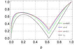
Figure 1: (color online). The indicator $\tau_{\alpha(3)}^{\left(1\right)}$ for the superposition state $\left|{\psi\left(p\right)}\right\rangle$ with $\alpha=0.83$ (green line), $\alpha=1$ (blue line), and $\alpha=1.1$ (red line). As an comparison, we also plot the three-tangle of $\left|{\psi\left(p\right)}\right\rangle$ with black line.

Example 2. Lohmayer et al found that there exists a kind of three-qubit mixed states loh06prl ,

$$\rho_{ABC}=p\left|{GHZ_{3}}\right\rangle\left\langle{GHZ_{3}}\right|+\left({1-p}\right)\left|{W_{3}}\right\rangle\left\langle{W_{3}}\right|$$ (21)

which is entangled but without two-qubit concurrence and three-tangle for the parameter $p\in[0.292,0.627]$. Now we use the indicator $\tau_{\alpha}^{1}$ to detect the genuine three-qubit entanglement in the mixed state. After some analysis, we obtain that the optimal pure state decomposition for $p\leq 0.627$ is $\rho_{ABC}=(F/3)\sum\limits_{j=0}^{2}{\left|{\psi^{j}\left({p_{0}}\right)}\right\rangle\left\langle{\psi^{j}\left({p_{0}}\right)}\right|}+\left({1-F}\right)\left|{W_{3}}\right\rangle\left\langle{W_{3}}\right|$ in which $F=p/p_{0}$ with $p_{0}=0.627$ and the component $\left|{\psi^{j}\left({p_{0}}\right)}\right\rangle=\sqrt{p_{0}}\left|{GHZ_{3}}\right\rangle-e^{(2\pi i/3)j}\sqrt{1-p_{0}}\left|{W_{3}}\right\rangle$. Then we can derive $\tau_{\alpha}^{\left(1\right)}\left({\rho_{A|BC}}\right)=F\tau_{\alpha}^{\left(1\right)}\left({\left|{\psi^{0}\left({p_{0}}\right)}\right\rangle}\right)+\left({1-F}\right)\tau_{\alpha}^{\left(1\right)}\left({\left|{W_{3}}\right\rangle}\right)$. In Fig.2, we plot the the indicator $\tau_{\alpha}^{\left(1\right)}\left({\rho_{ABC}}\right)$ as a function of parameters $p$ and $\alpha$. As shown in the figure, the values of this set of indicators are always positive, which detect the existence of the genuine three-qubit entanglement in the mixed state. It is noted that the case with the order $\alpha=1$ coincides with the result of the SEF-based indicator bxw14prl since the R$\alpha$E converge to the EOF in this case.

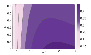
Figure 2: (color online). The indicator $\tau_{\alpha(3)}^{\left(1\right)}$ with the order $\alpha\in(0.83,3)$ detects the existence of the genuine three-qubit entanglement in the mixed state $\rho_{ABC}$ when the parameter $p\leq p_{0}$.

Example 3. The three-tangle based on the monogamy relation of the SC cannot detect the tripartite entanglement in the $W$ state. However, the SR$\alpha$E-based indication $\tau_{\alpha}^{(2)}$ can still work in this case. We consider the $N$-qubit $W$ state in the form $\left|{W_{N}}\right\rangle=1/\sqrt{N}\left({\left|{10\cdots 0}\right\rangle+\left|{01\cdots 0}\right\rangle+\cdots+\left|{00\cdots 1}\right\rangle}\right)$. When the quantum system is divided into $K$ parties with $K\in[3,4,\dots N]$, there are a set of hierarchical monogamy relations. The corresponding indicator can be written as $\tau_{\alpha\left(K\right)}({\left|{W_{N}}\right\rangle})=E_{\alpha}^{2}({C_{A_{1}|A_{2\cdots}A_{N}}^{2}})-({k-2})E_{\alpha}^{2}({C_{A_{1}A_{2}}^{2}})-E_{\alpha}^{2}({C_{A_{1}|A_{k\cdots}A_{N}}^{2}})$, where $C_{A_{1}|A_{2\cdots}A_{N}}^{2}=4(N-1)/N^{2},C_{A_{1}A_{2}}^{2}=4/N^{2}$, and $C_{A_{1}|A_{k\cdots}A_{N}}^{2}=4(N-k+1)/N^{2}$. In Table I, we calculate the indicator $\tau_{\alpha(K)}^{(2)}$ for a $7$-qubit $W$ state, where the party number $k$ ranges in $[3,7]$ and the order $\alpha$ is chosen as 0.95, 1, 1.05, 1.1, and 1.15. The nonzero values of this indicator reveal the multipartite entanglement in the $W$ state.

	$\alpha=0.95$	$\alpha=1$	$\alpha=1.05$	$\alpha=1.10$	$\alpha=1.15$
$k=3$	$0.0600$	$0.0626$	$0.0644$	$0.0656$	$0.0662$
$k=4$	$0.1136$	$0.1178$	$0.1205$	$0.1219$	$0.1225$
$k=5$	$0.1594$	$0.1642$	$0.1669$	$0.1680$	$0.1678$
$k=6$	$0.1954$	$0.2000$	$0.2021$	$0.2023$	$0.2010$
$k=7$	$0.2181$	$0.2219$	$0.2231$	$0.2222$	$0.2199$

Table 1: The values of the indicator $\tau_{\alpha\left(K\right)}\left({\left|{W_{7}}\right\rangle}\right)$ for the different party number $k$ and entanglement order $\alpha$.

IV Discussion and conclusion

We have considered the monogamy relations for the SR$\alpha$E in multiqubit systems. However, it is still an open problem that whether this result can be extended to the multi-level systems. Ou pointed out that the SC is not monogamous in a three-qutrit quantum state $\left|\psi\right\rangle_{ABC}=\left({\left|{123}\right\rangle}\right.-\left|{132}\right\rangle+\left|{231}\right\rangle-\left|{213}\right\rangle\left.{+\left|{312}\right\rangle-\left|{321}\right\rangle}\right)/\sqrt{6}$ ou07pra . When we use the monogamy relation of the SR$\alpha$E, it is found that

$$E_{\alpha}^{2}({\left|\psi\right\rangle_{A|BC}})-E_{\alpha}^{2}\left({\rho_{AB}}\right)-E_{\alpha}^{2}\left({\rho_{AC}}\right)\simeq 0.51211,$$ (22)

which is monogamous for an arbitrary value of the order $\alpha$. Next, we consider a four-partite mixed state $\rho_{A_{1}A_{2}A_{3}A_{4}}$ in $2\otimes d_{2}\otimes d_{3}\otimes d_{4}$ systems. Suppose that $C_{A_{1}|A_{2}A_{3}A_{4}}^{2}=0.7$, and $C_{A_{1}A_{2}}^{2}=C_{A_{1}A_{3}}^{2}=C_{A_{1}A_{4}}^{2}=0.35$. In this case, neither the SC or the SEF is monogamous and we have

$$C^{2}(\rho_{A_{1}|A_{2}A_{3}A_{4}})-\sum_{i=2}^{4}C^{2}(\rho_{A_{1}A_{i}})=-0.35$$

$$E_{f}^{2}(\rho_{A_{1}|A_{2}A_{3}A_{4}})-\sum_{i=2}^{4}E_{f}^{2}(\rho_{A_{1}A_{i}})=-0.037.$$ (23)

But the monogamy relation of the SR$\alpha$E still works for this mixed state and we can get

$$E_{\alpha}^{2}({\rho_{A_{1}|A_{2}A_{3}A_{4}}})-\sum_{i=2}^{4}{E_{\alpha}^{2}({\rho_{A_{1}A_{i}}})}=0.052,$$ (24)

where the order $\alpha=1.2$ has been chosen.

Beside the monogamy relations we have established in terms of the SR$\alpha$E, the similar relations can also be generalized to the $\mu$-th power of the R$\alpha$E. After some derivation, we can obtain the following theorem and its proof can be seen from Appendix C.

Theorem 4. For an arbitrary three-qubit mixed state ${\rho_{A_{1}A_{2}A_{3}}}$, the $\mu$-th power Rényi-$\alpha$ entanglement obeys the monogamy relation

$$E_{\alpha}^{\mu}\left({\rho_{A_{1}|A_{2}A_{3}}}\right)\geq E_{\alpha}^{\mu}\left({\rho_{A_{1}A_{2}}}\right)+E_{\alpha}^{\mu}\left({\rho_{A_{1}A_{3}}}\right)$$ (25)

where the order $\alpha\geq(\sqrt{7}-1)/2\simeq 0.823$ and the power $\mu\geq 2$. Moreover, in $N$-qubit systems, the following monogamy relation is also satisfied

$$E_{\alpha}^{\mu}({\rho_{A_{1}|A_{2\ldots}A_{n}}})\geq\sum\limits_{i=2}^{k-1}{E_{\alpha}^{\mu}({\rho_{A_{1}A_{i}}})}+E_{\alpha}^{\mu}(\rho_{A_{1}|A_{k}\dots A_{n}})$$ (26)

where the power $\mu\geq 2$ and the order $\alpha\in[\sqrt{7}-1)/2,(\sqrt{13}-1)/2]$.

We have thus proved the monogamy relation of the SR$\alpha$E in an arbitrary multi-qubit systems. Our results provide a broad class of new monogamy inequalities which include the previous result in terms of the SEF as a special case. Moreover, we have proved that the monogamy relations of the SR$\alpha$E possess a hierarchical structure when the $N$-qubit system is divided into $k$ parties. These new derived monogamy relations can be used to construct multipartite entanglement indicators in $N$-qubit systems, which still work well even when the corresponding ones based on the SC and SEF lose their efficacy. We also derived an analytical expression for the R$\alpha$E as a function of the SC in bipartite $2\otimes d$ systems. Finally, we analyze the monogamy property of the $\mu$-th power of Rényi-$\alpha$ entanglement. It is still an open problem yet to be answered that whether there exists a monogamy relation for the SR$\alpha$E in higher-dimensional systems .

Appendix A Proof of lemma 2

This lemma holds if the second-order derivative $\partial^{2}E_{\alpha}^{2}/\partial x^{2}>0$ for $\alpha\geq(\sqrt{7}-1)/2$. We first consider the squared Rényi-$\alpha$ entanglement for $\alpha\geq 1$. In this case, we define a function

$$h_{\alpha}=\frac{{\partial^{2}\left[{\left({1-\alpha}\right)^{2}E_{\alpha}^{2}}\right]}}{{\partial^{2}x^{2}}}$$ (27)

on the domain $\mathcal{D}=\left\{{\left({x,\alpha}\right)|0\leq x\leq 1,\alpha\geq 1}\right\}$ with $x$ being the squared concurrence. The nonnegativity of $h_{\alpha}$ can guarantee the nonnegative $\partial^{2}{E_{\alpha}^{2}}/\partial x^{2}$ since they are equivalent up to a positive constant. After some derivation, we have

$$h_{\alpha}\!=\!\Lambda\left\{{\alpha\left({A^{\alpha-1}\!-\!B^{\alpha-1}}\right)}\right.^{2}\!+\!\left[{\frac{{\left({B^{\alpha-1}\!-\!A^{\alpha-1}}\right)\left({A^{\alpha}\!+\!B^{\alpha}}\right)}}{{\sqrt{1-x}}}}\right.$$

$$\left.{\!+\!\left({\alpha-1}\right)\left({A^{\alpha-2}\!+\!B^{\alpha-2}}\right)\left({A^{\alpha}\!+\!B^{\alpha}}\right)-\alpha\left({A^{\alpha-1}\!-\!B^{\alpha-1}}\right)^{2}}\right]$$

$$\left.{\times\ln\left[{2^{-\alpha}\left({A^{\alpha}+B^{\alpha}}\right)}\right]}\right\}$$ (28)

where the parameter is $\Lambda=\alpha/2(A^{\alpha}+B^{\alpha})^{2}(1-x)(\ln 2)^{2}$ with $A=1+\sqrt{1-x}$ and $B=1-\sqrt{1-x}$. For the proof of the nonnegativity of $h_{\alpha}$, it is sufficient to analyze its maximal or minimal value on the domain $\mathcal{D}$. The critical points of $h_{\alpha}$ satisfy the condition

$$\nabla h_{\alpha}=\left({\frac{{\partial h_{\alpha}}}{{\partial x}},\frac{{\partial h_{\alpha}}}{{\partial\alpha}}}\right)=0.$$ (29)

In Fig.3 (a) and (b), we plot the solutions to equations $\partial h_{\alpha}/\partial x=0$ and $\partial h_{\alpha}/\partial\alpha=0$, respectively. As shown in the figure, the common solution is $\alpha=1$ which is on the boundary of the domain $\mathcal{D}$. Therefore, the maximal or minimal value of $h_{\alpha}$ can arise only on the boundary of domain $\mathcal{D}$. Next, we consider the other two boundaries $x=0$ and $x=1$ on the domain $\mathcal{D}$ of $h_{\alpha}$. When $x=0$, we have

$$\mathop{\lim}\limits_{x\to 0}h_{\alpha}=\frac{{{\alpha}^{2}}}{{8{\left({\ln 2}\right)^{2}}}}$$ (30)

which is always positive in the region $\alpha\in(1,+\infty)$. Similarly, when $x=1$, we can derive

$$\mathop{\lim}\limits_{x\to 1}h_{\alpha}=\frac{{(1-\alpha)^{2}\alpha\left[{3\alpha+2\left({\alpha^{2}+\alpha-3}\right)\ln 2}\right]}}{{6{\left({\ln 2}\right)^{2}}}}$$ (31)

which is monotonically increasing and positive in the region $\alpha\in(1,+\infty)$. Notice that the critical points arise only on the boundary of domain $\mathcal{D}$, we obtain that the function $h_{\alpha}$ is nonnegative in the whole range ${0\leq x\leq 1,\alpha\geq 1}$ (the equality holds only at the boundary $\alpha=1$). In Fig. 4, we plot $h_{\alpha}$ as a function of $x$ and $\alpha$, which illustrates our result. According to the equivalent relation in Eq. (27), we have $\partial^{2}E_{\alpha}^{2}/\partial x^{2}>0$ for $\alpha>1$. When $\alpha=1$, $E^{2}_{\alpha}$ converges to SEF and its second-order derivative is positive bxw14prl . Therefore, the second-order derivative of $E^{2}_{\alpha}$ is positive for $\alpha\geq 1$.

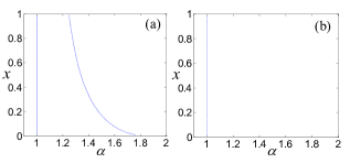
Figure 3: (color online). The plot of the dependence of $x$ with $\alpha$ which satisfies the equation (a)$\frac{{\partial h_{\alpha}}}{{\partial x}}=0$ and (b)$\frac{{\partial h_{\alpha}}}{{\partial\alpha}}=0$ respectively.

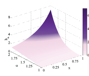
Figure 4: (color online). The function ${h_{\alpha}}$ is plotted as a function of $x$ and $\alpha$ for $0\leq x\leq 1,\alpha\geq 1$, which is positive, and as a result, the SR$\alpha$E is a convex function of SC.

We further analyze the nonnegative region for the second-order derivative $\partial^{2}E_{\alpha}^{2}/\partial x^{2}$ when $\alpha$ ranges in $(0,1)$. It is found that, under the condition $\partial^{2}E_{\alpha}^{2}/\partial x^{2}=0$, the critical value of $x$ increases monotonically along with the parameter $\alpha$. In Fig.5(a), we plot the solution $(x,\alpha)$ to this critical condition, where for each fixed $x$ there exists a value of $\alpha$ such that the second-order derivative of $E_{\alpha}^{2}$ is zero. Due to $x$ varying monotonically with $\alpha$, we only need consider the condition $\partial^{2}E_{\alpha}^{2}/\partial x^{2}=0$ in the limit $x\to 1$. In this case, we have the derivative

$$\mathop{\lim}\limits_{x\to 1}\frac{{\partial^{2}E_{\alpha}^{2}}}{{\partial x^{2}}}=\frac{{\alpha\left[{3\alpha+2\left({\alpha^{2}+\alpha-3}\right)\ln 2}\right]}}{{6{\left({\ln 2}\right)^{2}}}}=0,$$ (32)

which gives the critical point $\alpha_{c_{1}}=[-(2\ln 2+3)+\sqrt{(2\ln 2+3)^{2}+48(\ln 2)^{2}}]/4\ln 2\simeq 0.764$. When $\alpha\geq\alpha_{c_{1}}$, the second-order $\partial^{2}E_{\alpha}^{2}/\partial x^{2}$ is always positive. Notice that the analytical formula $E_{\alpha}(C^{2})$ in Eq.(5) is established only for $\alpha\geq(\sqrt{7}-1)/2=\alpha_{c}$, we have $\partial^{2}E_{\alpha}^{2}/\partial x^{2}>0$ for $\alpha\in[\alpha_{c},1)$.

Combining the two positive regions $[\alpha_{c},1)$ and $[1,+\infty)$, we obtain the derivative $\partial^{2}E_{\alpha}^{2}/\partial x^{2}>0$ for $\alpha\geq(\sqrt{7}-1)/2$, which completes the proof of lemma 2.

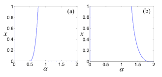
Figure 5: (color online). The plot of the dependence of $x$ with $\alpha$ using the equation (a)$\frac{{\partial^{2}E_{\alpha}^{2}}}{{\partial x^{2}}}=0$, (b)$\frac{{\partial^{2}E_{\alpha}}}{{\partial x^{2}}}=0$.

Appendix B Proof of lemma 3

The R$\alpha$E $E_{\alpha}$ is monotonically increasing if the first-order derivative $\partial E_{\alpha}/\partial x>0$ with $x$ being the squared concurrence. After some calculation, we have

$$\frac{{\partial E_{\alpha}}}{{\partial x}}=\frac{{\alpha\left({B^{\alpha-1}-A^{\alpha-1}}\right)}}{{2\left({1-\alpha}\right)\left({A^{\alpha}+B^{\alpha}}\right)\sqrt{1-x}\ln 2}}$$ (33)

where the parameters are $A=1+\sqrt{1-x}$ and $B=1-\sqrt{1-x}$. It is easy to verify the derivative is nonnegative in the regions $\alpha\in\left[{0,1}\right)$ and $\alpha\in\left({1,+\infty}\right)$. Combining the two regions with the case $\alpha=1$ which was proved in Ref. bxw14pra , we obtain that the first-order derivative of ${E_{\alpha}}$ is always nonnegative for $\alpha\geq 0$ and the equality holds only at the boundary of $x$. Therefore, the R$\alpha$E is monotonically increasing.

Furthermore, the concave property of ${E_{\alpha}}$ as a function of ${C^{2}}$ holds if the second-order derivative $\partial^{2}E_{\alpha}/\partial x^{2}<0$ with $x$ being the squared concurrence. In order to determinate the region of $\alpha$, we analyze the condition $\partial^{2}E_{\alpha}/\partial x^{2}=0$. It is found that the value of $x$ decreases monotonically along with the increase of $\alpha$. In Fig. 5(b), we plot the relation between $x$ and $\alpha$ under this condition. As shown in the figure, the critical point corresponds to the limit

$$\mathop{\lim}\limits_{x\to 1}\frac{{\partial^{2}E_{\alpha}}}{{\partial x^{2}}}=\frac{{\alpha\left({\alpha^{2}+\alpha-3}\right)}}{{6\ln 2}}=0.$$ (34)

After some calculation, we can obtain that the critical point is $\alpha_{c_{2}}=(\sqrt{13}-1)/2\simeq 1.303$. Therefore, the second-order derivative is negative when $\alpha<\alpha_{c_{2}}$. It is noted that the analytical formula $E_{\alpha}(C^{2})$ hold for $\alpha\geq(\sqrt{7}-1)/2$. Thus we can get $\partial^{2}E_{\alpha}/\partial x^{2}\leq 0$ for $\alpha\in[(\sqrt{7}-1)/2,(\sqrt{13}-1)/2]$ (the equality holds only at the right boundary), which results in the concave property of $E_{\alpha}(C^{2})$. The proof of lemma 3 is completed.

Appendix C Proof of theorem 4

According to theorem 1, we have

$$E_{\alpha}^{2}({\rho_{A_{1}|A_{2}A_{3}}})\geq E_{\alpha}^{2}({\rho_{A_{1}A_{2}}})+E_{\alpha}^{2}({\rho_{A_{1}A_{3}}})$$ (35)

for $\alpha\geq(\sqrt{7}-1)/2$. Without loss of generality, we assume the two-qubit entanglement $E_{\alpha}({\rho_{A_{1}A_{2}}})\geq E_{\alpha}({\rho_{A_{1}A_{3}}})$. Then we can get

$$E_{\alpha}^{\mu}\left({\rho_{A_{1}|A_{2}A_{3}}}\right) \geq \left({E_{\alpha}^{2}\left({\rho_{A_{1}A_{2}}}\right)+E_{\alpha}^{2}\left({\rho_{A_{1}A_{3}}}\right)}\right)^{\frac{\mu}{2}}$$ (36)

$$= E_{\alpha}^{\mu}\left({\rho_{A_{1}A_{2}}}\right)\left({1+\frac{{E_{\alpha}^{2}\left({\rho_{A_{1}A_{3}}}\right)}}{{E_{\alpha}^{2}\left({\rho_{A_{1}A_{2}}}\right)}}}\right)^{\frac{\mu}{2}}$$

$$\geq E_{\alpha}^{\mu}\left({\rho_{A_{1}A_{2}}}\right)\left({1+\left({\frac{{E_{\alpha}^{2}\left({\rho_{A_{1}A_{3}}}\right)}}{{E_{\alpha}^{2}\left({\rho_{A_{1}A_{2}}}\right)}}}\right)^{\frac{\mu}{2}}}\right)$$

$$= E_{\alpha}^{\mu}\left({\rho_{A_{1}A_{2}}}\right)+E_{\alpha}^{\mu}\left({\rho_{A_{1}A_{3}}}\right)$$

where in the third inequality we have used the property $\left({1+x}\right)^{t}\geq 1+x^{t}$, for $x\leq 1,t\geq 1$.

For the monogamy relation of $\mu$-th power in $N$-qubit systems, we first consider a tripartite mixed state in $2\otimes 2\otimes 2^{N-2}$ systems. According to theorem 3, the tripartite monogamy relation for the squared R$\alpha$E is satisfied. Then, using the same technique in Eq. (35), we can obtain the $\mu$-th power monogamy inequality. Furthermore, by the successive cut for the last party and application of the tripartite monogamy relation, we can derive the $k$-partite inequality as shown in Eq. (26) of the main text.

References

(1) R. Horodecki, P. Horodecki, M. Horodecki, and K. Horodecki, Rev. Mod. Phys.
81, 865 (2009).
(2) C. H. Bennett, H. J. Bernstein, S. Popescu, and B. Schumacher, Phys. Rev. A
53, 2046 (1996).
(3) W. K. Wootters, Phys. Rev. Lett. 80, 2245 (1998).
(4) V. Coffman, J. Kundu, and W. K. Wootters, Phys. Rev. A 61, 052306
(2000).
(5) T. J. Osborne, and F. Verstraete, Phys. Rev. Lett. 96, 220503 (2006).
(6) Y.-K. Bai, D. Yang, and Z. D. Wang, Phys. Rev. A 76, 022336 (2007).
(7) Y.-K. Bai, and Z. D. Wang, Phys. Rev. A 77, 032313 (2008).
(8) Y.-C. Ou, H. Fan, and S.-M. Fei, Phys. Rev. A 78, 012311 (2008).
(9) E. Jung, D. Park, and J.-W. Son, Phys. Rev. A 80, 010301(2009).
(10) C. Eltschka, A. Osterloh, and J. Siewert, Phys. Rev. A 80,
032313 (2009).
(11) X.-J. Ren, and W. Jiang, Phys. Rev. A 81, 024305 (2010).
(12) M. F. Cornelio, Phys. Rev. A 87, 032330 (2013).
(13) B. Regula, S. D. Martino, S. Lee, and G. Adesso, Phys. Rev. Lett. 113,
110501 (2014).
(14) J. S. Kim, Phys.Rev.A 90, 062306 (2014).
(15) Y.-K. Bai, M.-Y. Ye, and Z. D. Wang, Phys. Rev. A 80, 044301 (2009)
(16) G. H. Aguilar, A. Valdés-Hernández, L. Davidovich, S. P. Walborn, and
P. H. Souto Ribeiro, Phys. Rev. Lett. 113, 240501 (2014).
(17) C.-S. Yu and H.-S. Song, Phys. Rev. A 71, 042331 (2005).
(18) D. Yang, Phys. Lett. A 360, 249 (2006).
(19) D. P. Chi, J. W. Choi, K. Jeong, J. S. Kim, T. Kim, and S. Lee, J. Math. Phys.
(N.Y.) 49, 112102 (2008).
(20) C.-S. Yu, and H.-S. Song, Phys. Rev. A 77, 032329 (2008).
(21) A. Kay, D. Kaszlikowski, and R. Ramanathan, Phys. Rev. Lett. 103,
050501 (2009).
(22) A. García-Sáez and J. I. Latorre, Phys. Rev. B 87, 085130
(2013).
(23) A. Osterloh and R. Schutzhold, Phys. Rev. B 91, 125114 (2015).
(24) C. Eltschka, and J. Siewert, Phys. Rev. Lett. 114, 140402 (2015).
(25) G. Adesso, and F. Illuminati, New J. Phys. 8, 15 (2006).
(26) T. Hiroshima, G. Adesso, and F. Illuminati, Phys. Rev. Lett. 98,
050503 (2007).
(27) G. Adesso and F. Illuminati, Phys. Rev. Lett. 99, 150501 (2007).
(28) M. Koashi, and A. Winter, Phys. Rev. A 69, 022309 (2004).
(29) M. Christandl, and A. Winter, J. Math. Phys. (N.Y.) 45, 829 (2004).
(30) Dong Yang, K. Horodecki, M. Horodecki, P. Horodecki, J. Oppenheim, and Wei Song,
IEEE. Tran. Info. Theory, 55, 3375 (2009).
(31) Y.-C. Ou and H. Fan, Phys. Rev. A 75, 062308 (2007).
(32) J. S. Kim, A. Das, and B. C. Sanders, Phys. Rev. A 79, 012329 (2009).
(33) H. He, and G. Vidal, Phys. Rev. A 91, 012339 (2015).
(34) J. H. Choi and J. S. Kim, Phys. Rev. A 92, 042307 (2015).
(35) Y. Luo and Y. Li, Ann. Phys. 362, 511 (2015).
(36) J. S. Kim, and B. C. Sanders, J. Phys. A: Math. Theor. 43, 445305
(2010).
(37) M. F. Cornelio and M. C. de Oliveira, Phys.Rev.A 81, 032332 (2010).
(38) R. Lohmayer, A. Osterloh, J. Siewert, and A. Uhlmann, Phys. Rev. Lett.
97, 260502 (2006).
(39) Y.-K. Bai, M.-Y. Ye, and Z. D. Wang, Phys. Rev. A 78 062325 (2008).
(40) Y.-K. Bai, N. Zhang, M.-Y. Ye, and Z. D. Wang, Phys. Rev. A 88,
012123 (2013).
(41) T. R. de Oliveira, M. F. Cornelio, and F. F. Fanchini, Phys. Rev. A
89, 034303 (2014).
(42) Y.-K. Bai, Y.-F. Xu, and Z. D. Wang, Phys. Rev. Lett. 113,
100503 (2014).
(43) X.-N. Zhu and S.-M. Fei, Phys. Rev. A 90, 024304 (2014).
(44) Y.-K. Bai, Y.-F. Xu, and Z. D. Wang, Phys. Rev. A 90, 062343 (2014).
(45) F. Liu, F. Gao, and Q.-Y. Wen, Sci. Rep. 5, 16745 (2015).
(46) R. Horodecki, P. Horodecki, and M. Horodecki, Phys. Lett. A 210,
377 (1996).
(47) J. Cui, M. Gu, L. C. Kwek, M. F. Santos, H. Fan, and V. Vedral, Nature Commun.
3, 812 (2012).
(48) F. Franchini, J. Cui, L. Amico, H. Fan, M. Gu, L. C. Kwek, V. Korepin, and V.
Vedral, Phys. Rev. X 4, 041028 (2014).
(49) S. T. Flammia, A. Hamma, T. L. Hughes, and X. G. Wen, Phys. Rev. Lett.
103, 261601 (2009).
(50) G. B. Halasz, and A. Hamma, Phys. Rev. Lett. 110, 170605 (2013).
(51) A. Hamma, L. Cincio, S. Santra, P. Zanardi, and A. Luigi, Phys. Rev. Lett.
110, 210602 (2013).
(52) J. Cui, L Amico, H. Fan, M. Gu, A. Hamma, and V. Vedral, Phys. Rev. B
88 125117 (2013).
(53) Yu-Xin Wang, Liang-Zhu Mu, and V. Vedral, and Heng Fan, arXiv:1504.03909.