Abstract

Using posterior distribution of Bayesian LASSO we construct a semi-norm on the parameter space. We show that the partition function depends on the ratio of the $l^{1}$ and $l^{2}$ norms and present three regimes. We derive the concentration of Bayesian LASSO, and present MCMC convergence diagnosis.

keyword: LASSO, Bayes, MCMC, log-concave, geometry, incomplete Gamma function

1 Introduction

Let $p\geq n$ be two positive integers, $\boldsymbol{y}\in\mathbb{R}^{n}$ and $\mathbf{A}$ be an $n\times p$ matrix with real numbers entries. Bayesian LASSO

$$c(\boldsymbol{x})=\frac{1}{Z}\exp\Big{(}-\frac{\|\mathbf{A}\boldsymbol{x}-\boldsymbol{y}\|_{2}^{2}}{2}-\|\boldsymbol{x}\|_{1}\Big{)}$$ (1)

is a typically posterior distribution used in the linear regression

$$\boldsymbol{y}=\mathbf{A}\boldsymbol{x}+\boldsymbol{w}.$$

Here

$$Z=\int_{\mathbb{R}^{p}}\exp\Big{(}-\frac{\|\mathbf{A}\boldsymbol{x}-\boldsymbol{y}\|_{2}^{2}}{2}-\|\boldsymbol{x}\|_{1}\Big{)}d\boldsymbol{x}$$ (2)

is the partition function, $\|\cdot\|_{2}$ and $\|\cdot\|_{1}$ are respectively the Euclidean and the $l_{1}$ norms. The vector $\boldsymbol{y}\in\mathbb{R}^{n}$ are the observations, $\boldsymbol{x}\in\mathbb{R}^{p}$ is the unknown signal to recover, $\boldsymbol{w}\in\mathbb{R}^{n}$ is the standard Gaussian noise, and $\mathbf{A}$ is a known matrix which maps the signal domain $\mathbb{R}^{p}$ into the observation domain $\mathbb{R}^{n}$. If we suppose that $\boldsymbol{x}$ is drawn from Laplace distribution i.e. the distribution proportional to

$$\exp(-\|\boldsymbol{x}\|_{1}),$$ (3)

then the posterior of $\boldsymbol{x}$ known $y$ is drawn from the distribution $c$ (1). The mode

$$\arg\min\Big{\{}\frac{\|\mathbf{A}\boldsymbol{x}-\boldsymbol{y}\|_{2}^{2}}{2}+\|\boldsymbol{x}\|_{1}:\quad\boldsymbol{x}\in\mathbb{R}^{p}\Big{\}}$$ (4)

of $c$ was first introduced in [14] and called LASSO. It is also called Basis Pursuit De-Noising method [4]. In our work we select the term LASSO and keep it for the rest of the article.

In general LASSO is not a singleton, i.e. the mode of the distribution $c$ is not unique. In this case LASSO is a set and we will denote by lasso any element of this set. A large number of theoretical results has been provided for LASSO. See [5], [6], [8], [12] and the references herein. The most popular algorithms to find LASSO are LARS algorithm [7], ISTA and FISTA algorithms see e.g. [2] and the review article [10].

The aim of this work is to study geometry of bayesian LASSO and to derive MCMC convergence diagnosis.

2 Polar integration

Using polar coordinates, the partition function (2)

$$Z=\int_{S}J_{p}(\theta)d\theta,$$ (5)

where $d\theta$ denotes the surface measure on the unit sphere $S$, and

$$J_{p}(\theta)=\int_{0}^{+\infty}\exp(-g(r,\theta))r^{p-1}dr.$$ (6)

Here

$$g(r,\theta)=\frac{1}{2}(r^{2}\|\mathbf{A}\theta\|_{2}^{2}+2r\|\mathbf{A}\theta\|_{2}\beta+\|\boldsymbol{y}\|_{2}^{2}),$$ (7)

where

$$\beta:=\frac{\|\theta\|_{1}}{\|\mathbf{A}\theta\|_{2}}-\|\boldsymbol{y}\|_{2}s,$$ (8)

and $s$ denotes the cosine of the angle $(\mathbf{A}\theta,\boldsymbol{y})$ i.e. $\cos((\mathbf{A}\theta,\boldsymbol{y}))$ . Using known estimate $\|\theta\|_{2}\leq\|\theta\|_{1}$, we observe that $\beta$ is bounded below by

$$\frac{1}{\|\mathbf{A}\|}-\|\boldsymbol{y}\|_{2},$$ (9)

and $\beta\to+\infty$ as $\mathbf{A}\theta\to 0$. Here $\|\mathbf{A}\|$ is the square root of the largest eigenvalue of $\mathbf{A}^{*}\mathbf{A}$. Observe that

$$c(\boldsymbol{x})d\boldsymbol{x}=\frac{1}{Z}\exp(-g(r,\theta))r^{p-1}drd\theta.$$

Hence, we can sample from Bayesian LASSO $c$ (1) as following. We draw uniformly $\theta:=\frac{\boldsymbol{x}}{\|\boldsymbol{x}\|_{2}}$ from the unit sphere, and then draw the norm $\|\boldsymbol{x}\|_{2}$ following the distribution

$$\mu_{\theta}(r):=\frac{1}{J_{p}(\theta)}\exp(-\varphi(r,\theta)),$$ (10)

where

$$\varphi(r,\theta):=g(r,\theta)-(p-1)\ln(r),\quad r>0.$$ (11)

Moreover, observe that the modes $\{\boldsymbol{x}_{lasso}=r_{lasso}\theta_{lasso}:\quad g(r_{lasso},\theta_{lasso})=\min_{r\geq 0,\theta\in S}g(r,\theta)\}$ and $\{(r^{*},\theta^{*}):\quad\varphi(r,\theta)=\min_{r\geq 0,\theta\in S}\varphi(r,\theta)\}$ respectively of the distributions $c(\boldsymbol{x})d\boldsymbol{x}$ and $\frac{1}{Z}\exp(-g(r,\theta))r^{p-1}drd\theta$ are different. We will show that $(r^{*},\theta^{*})$ contains more information than $\boldsymbol{x}_{lasso}$.

3 Geometric interpretation of the partition function

The volume (Lebesgue measure) of the set $K(\mathbf{A},\boldsymbol{y}):=\{\boldsymbol{x}\in\mathbb{R}^{p}:J_{p}(\boldsymbol{x})\geq 1\}$ is $vol(K(\mathbf{A},\boldsymbol{y}))=\frac{1}{p}Z$. Observe that $J_{p}^{-\frac{1}{p}}$ is a norm on the null-space $N(\mathbf{A})$ of $\mathbf{A}$. A general result [1] tells us that if $f$ is even, log-concave and integrable on an Euclidean space $E$, then

$$\boldsymbol{x}\in E\to(\int_{0}^{+\infty}f(r\boldsymbol{x})r^{p-1}dr)^{-\frac{1}{p}}$$

is a norm on $E$. It follows that in the case $E=N(\mathbf{A})$ or $E=\{\boldsymbol{x}\in\mathbb{R}^{p}:\langle\mathbf{A}\boldsymbol{x},\boldsymbol{y}\rangle=0\}$, the map

$$\boldsymbol{x}\in E\to J_{p}^{-\frac{1}{p}}(\boldsymbol{x})$$

is a norm on $E$. The map

$$\boldsymbol{x}\in\mathbb{R}^{p}\to J_{p}^{-\frac{1}{p}}(\boldsymbol{x}):=\|\boldsymbol{x}\|_{LASSO}$$

has nearly all the properties of a norm. Only the evenness is missing. The set $K(\mathbf{A},\boldsymbol{y})=\{\boldsymbol{x}\in\mathbb{R}^{p}:\quad\|\boldsymbol{x}\|_{LASSO}\leq 1\}$ is convex, compact and contains the origin. See [9] for more details.

3.1 Necessary and sufficient condition to have $LASS0=\{0\}$

If $\beta\geq 0$, then $r\in[0,+\infty)\to g(r,\theta)$ is increasing, its minimizer is equal to $r=0$, and its smallest value is $\frac{\|\boldsymbol{y}\|_{2}^{2}}{2}$. If $\beta<0$, then its minimizer is equal to $r=-\frac{\beta}{\|\mathbf{A}\theta\|_{2}}$, and its smallest value is less than $\frac{\|\boldsymbol{y}\|_{2}^{2}}{2}$. If the set $\{\beta<0\}$ is empty, then $LASSO=\{0\}$, if not

$$LASSO=\{\boldsymbol{l}=-\frac{\beta_{l}}{\|\mathbf{A}\theta_{l}\|_{2}}\theta_{l}:\quad\beta_{l}\leq 0,\,\mbox{s.t.}\,\beta_{l}^{2}=\sup_{\beta\leq 0}\beta^{2}\}.$$ (12)

As an illustration we consider the case $n=4$, $p=7$ and the entries of the matrix $\mathbf{A}\sim\mathcal{B}(\pm\frac{1}{\sqrt{n}})$ are a realization of i.i.d. Bernoulli random variables with the values $\pm\frac{1}{\sqrt{n}}$. We draw uniformly $N=10^{5}$ vectors from the sphere $S$ and estimate LASSO using Formula (12). Table 1 gives the value of LASSO using respectively FISTA algorithm and Formula (12).

	$x_{1}$	$x_{2}$	$x_{3}$	$x_{4}$	$x_{5}$	$x_{6}$	$x_{7}$
$LASSO_{FISTA}$	1.7744	0.6019	-0.3283	0	0	-1.0050	0
$LASSO_{POLAR}$	0.9992	0.3890	-1.3980	0.0769	-0.0070	-0.8699	-0.0379

Table 1: $N=10^{5}$, $p=7$, $n=4$.

Observe that necessary and sufficient condition for $\beta\geq 0$ for all $\theta$ is

$$\|\boldsymbol{y}\|_{2}\leq\inf\{\frac{\|\theta\|_{1}}{\|\mathbf{A}\theta\|_{2}|s|}:\quad\theta\in S\}.$$

Using known estimate $\|\theta\|_{2}\leq\|\theta\|_{1}$, we obtain

$$\|\boldsymbol{y}\|_{2}\leq\frac{1}{\|\mathbf{A}\|}$$

as a sufficient condition for $\beta\geq 0$ for all $\theta$.

4 Closed form of the partition function

We introduce for $a\in\mathbb{R}$ and for a couple $p,r\geq 1$ of integers, the notations

$$(a)_{r} = (a-1)\ldots(a-r),$$ (13)

$$c(p,r) = \sum_{k=0}^{p-1}\binom{p-1}{k}(-1)^{p-1-k}(\frac{k+1}{2})_{r}.$$ (14)

Now, we can announce the following result.

Proposition 4.1.

1) If $\beta=+\infty$, then

$$\|\theta\|_{1}^{p}J_{p}(\theta)=(p-1)!\exp(-\frac{\|\boldsymbol{y}\|_{2}^{2}}{2}).$$

2) If $\beta\geq 0$, then

$$\|\theta\|_{1}^{p}J_{p}(\theta):=\Phi(\beta),$$

where

$$\Phi(\beta)= \exp(-\frac{\|\boldsymbol{y}\|_{2}^{2}}{2})(\beta+s\|\boldsymbol{y}\|_{2})^{p}\sum_{k=0}^{p-1}\binom{p-1}{k}(-\beta)^{p-1-k}$$ (15)

$$2^{\frac{k-1}{2}}\exp(\frac{\beta^{2}}{2})\Gamma(\frac{k+1}{2},\frac{\beta^{2}}{2}),$$

Here $\Gamma(a,x)=\int_{x}^{+\infty}\exp(-t)t^{a-1}dt,\quad a>0,x\geq 0$, is the upper incomplete Gamma function.

3) If $\beta<0$, then

$$\|\theta\|_{1}^{p}J_{p}(\theta)= \exp(-\frac{\|\boldsymbol{y}\|_{2}^{2}}{2})(\beta+s\|\boldsymbol{y}\|_{2})^{p}\sum_{k=0}^{p-1}\binom{p-1}{k}(-\beta)^{p-1-k}$$ (16)

$$2^{\frac{k-1}{2}}\exp(\frac{\beta^{2}}{2})2^{\frac{k-1}{2}}(\Gamma(\frac{k+1}{2})+(-1)^{k}\gamma(\frac{k+1}{2},\frac{\beta^{2}}{2})).$$

Here $\gamma(a,x)=\int_{0}^{x}\exp(-t)t^{a-1}dt$ is the lower incomplete Gamma function.

4) If $\beta=0$, then

$$\|\theta\|_{1}^{p}J_{p}(\theta)=\exp(-\frac{\|\boldsymbol{y}\|_{2}^{2}}{2})2^{\frac{p-2}{2}}\|\boldsymbol{y}\|_{2}^{p}s^{p}\Gamma(\frac{p}{2},0).$$

5) If $\beta>0$ then for $M\geq p+1$,

$$\|\theta\|_{1}^{p}J_{p}(\theta):=\Phi(\beta,M)+R(\beta,M),$$

where

$$\Phi(\beta,M)=(p-1)!\exp(-\frac{\|\boldsymbol{y}\|_{2}^{2}}{2})+\sum_{r=p}^{M-1}2^{p-1}\exp(-\frac{\|\boldsymbol{y}\|_{2}^{2}}{2})\Big{(}1+\frac{\|\boldsymbol{y}\|_{2}s}{\beta}\Big{)}^{p}c(p,r)\Big{(}\frac{\beta^{2}}{2}\Big{)}^{p-1-r}$$ (17)

and the remainder term

$$|R(\beta,M)|\leq\Big{(}1+\frac{\|\boldsymbol{y}\|_{2}s}{\beta}\Big{)}^{p}\exp(-\frac{\|\boldsymbol{y}\|_{2}^{2}}{2})2^{p-1}\frac{|c(p,M)|}{\Big{(}\frac{\beta^{2}}{2}\Big{)}^{M-(p-1)}}$$ (18)

Proof 4.2.

Only the first part of assertions 2) and 5) needs the proof. Let us prove the first part of 2). From the equality

$$J_{p}(\theta)=\exp(-\frac{\|\boldsymbol{y}\|_{2}^{2}}{2}+\frac{\beta^{2}}{2})\int_{0}^{+\infty}\exp(-\frac{(\|\mathbf{A}\theta\|_{2}r+\beta)^{2}}{2})r^{p-1}dr,$$

and the change of the variable

$$\tau=\|\mathbf{A}\theta\|_{2}r+\beta,$$

we obtain

$$\int_{0}^{+\infty}\exp\Big{(}-\frac{(\|\mathbf{A}\theta\|_{2}r+\beta)^{2}}{2}\Big{)}r^{p-1}dr = \frac{1}{\|\mathbf{A}\theta\|_{2}^{p}}\int_{\beta}^{+\infty}\exp(-\frac{\tau^{2}}{2})(\tau-\beta)^{p-1}d\tau$$

$$= \frac{1}{\|\mathbf{A}\theta\|_{2}^{p}}\sum_{k=0}^{p-1}\binom{p-1}{k}(-\beta)^{p-1-k}\int_{\beta}^{+\infty}\exp(-\frac{\tau^{2}}{2})\tau^{k}d\tau.$$

As $\beta>0$, then the change of variable

$$\omega=\frac{\tau^{2}}{2},$$

implies

$$\int_{\beta}^{+\infty}\exp(-\frac{\tau^{2}}{2})\tau^{k}d\tau=2^{\frac{k-1}{2}}\Gamma(\frac{k+1}{2},\frac{\beta^{2}}{2}).$$

The equality $\beta=\frac{\|\theta\|_{1}}{\|\mathbf{A}\theta\|_{2}}-\|\boldsymbol{y}\|_{2}s$ achieves the proof of 2).

Now we prove Assertion 5). We extend the incomplete Gamma function as following

$$\Gamma(a,x)=\int_{x}^{+\infty}\exp(-t)t^{a-1}dt,\quad x>0,a\in\mathbb{R},$$

and we use known estimate see [3] page 14

$$\Gamma(a,x)=\exp(-x)x^{a-1}+\sum_{r=1}^{M-1}(a)_{r}\exp(-x)x^{a-1-r}+R(a,x,M),$$ (19)

where $M>a-1$, $x>0$, $a\in\mathbb{R}$, and the remainder term

$$|R(a,x,M)|\leq(a)_{M-1}\exp(-x)x^{a-1-M}.$$

If $\beta>0$, then from $\beta=\frac{\|\theta\|_{1}}{\|\mathbf{A}\theta\|_{2}}-\|\boldsymbol{y}\|_{2}s$, we have

$$J_{p}(\theta)= \frac{2^{p-1}}{\|\theta\|_{1}^{p}}\exp(-\frac{\|\boldsymbol{y}\|_{2}^{2}}{2})\Big{(}1+\frac{\|\boldsymbol{y}\|_{2}s}{\beta}\Big{)}^{p}\Big{(}\frac{\beta^{2}}{2}\Big{)}^{p-1}\sum_{k=0}^{p-1}\binom{p-1}{k}(-1)^{p-1-k}$$

$$\exp(\frac{\beta^{2}}{2})\Big{(}\frac{\beta^{2}}{2}\Big{)}^{-\frac{k-1}{2}}\Gamma(\frac{k+1}{2},\frac{\beta^{2}}{2}).$$

Using the expansion (19), and the fact that $J_{p}(\theta)\to\frac{(p-1)!}{\|\theta\|_{1}^{p}}\exp(-\frac{\|\boldsymbol{y}\|_{2}^{2}}{2})$ as $\beta\to+\infty$, we obtain for $r<p-1$

$$c(p,r)=0,\quad 1\leq r<p-1,\quad c(p,p-1)=\frac{(p-1)!}{2^{p-1}}.$$

It follows the following expansion:

$$\Big{(}1+\frac{\|\boldsymbol{y}\|_{2}s}{\beta}\Big{)}^{-p}\|\theta\|_{1}^{p}\exp(\frac{\|\boldsymbol{y}\|_{2}^{2}}{2})J_{p}(\theta)=(p-1)!+2^{p-1}\sum_{r=p}^{M-1}\frac{c(p,r)}{\Big{(}\frac{\beta^{2}}{2}\Big{)}^{r-(p-1)}}+\tilde{R}(\beta,M),$$

where the remainder term

$$|\tilde{R}(\beta,M)|\leq 2^{p-1}\frac{|c(p,M)|}{\Big{(}\frac{\beta^{2}}{2}\Big{)}^{M-(p-1)}},$$

which achieves the proof.

4.1 Numerical calculations

As an illustration we consider $n=4$, $p=7$, $\mathbf{A}\sim\mathcal{B}(\pm\frac{1}{\sqrt{n}})$, and $\boldsymbol{y}=0$. The choice $M=17$ corresponds to the relative error $\frac{|R(\beta,M)|}{|\Phi(\beta,M)|}\leq 10^{-4}$ for $\beta\geq 7.5$.

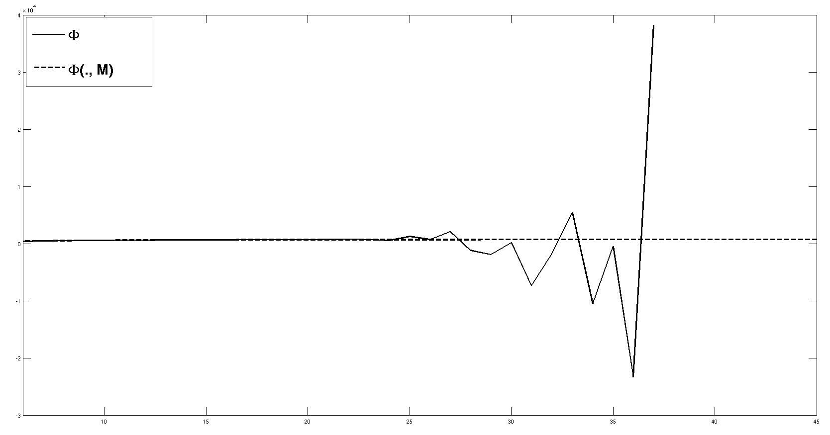
Figure 1: Curves of $\Phi(\beta)$ and $\Phi(\beta,17)$, $\beta=[6,45]$, $p=7$, $n=4$.

Numerical calculations show that the function $\Phi(\beta)$ (15) explodes for $\beta>13.8$. To compass these explosions we use the expansion (19), and then we use the function $\Phi(\cdot,M)$ (17). In Fig.(1) and Fig.(2) dashed and black curves represent respectively the function $\Phi(\cdot,M)$ and $\Phi$. In Fig. (1) we plot $\Phi(\cdot,M)$ and $\Phi$ for $\beta\in(6,45)$. By zooming on $\beta\in(1.09,7.5)$, $\beta\in(7.5,13.8)$, and $\beta\in(13.8,15)$ we show that the behavior of $\Phi$ becomes abnormal from $\beta\approx\beta_{\Phi}=13.8$ and obtain Fig.(2).

4.2 The case LASS0={ 0 }: Partition function estimate and concentration inequality

The following is a consequence of [9] Lemma 2.1.

Proposition 4.3.

1) The function $r\in(0,+\infty)\to\varphi(r,\theta)$ is convex and its unique critical point

$$r(\theta)=\frac{-\beta+\sqrt{\beta^{2}+4(p-1)}}{2\|\mathbf{A}\theta\|_{2}}$$ (20)

is the mode of (10).

2) By denoting $M(\theta)=\exp\Big{(}-\varphi(r(\theta),\theta)\Big{)}$, we obtain

$$\frac{M(\theta)r(\theta)}{p}\leq J_{p}(\theta)\leq\frac{M(\theta)r(\theta)(p-1)!\exp(p-1)}{(p-1)^{p}}.$$

3) We have for $q>0$,

$$\int_{qr(\theta)}\exp(-\varphi(r,\theta))dr\leq\frac{p\Gamma(p,(p-1)q)\exp(p-1)}{(p-1)^{p}}\int_{0}^{+\infty}\exp(-\varphi(r,\theta))dr,$$

and

$$Z_{min}:=\frac{|S|\inf_{\theta\in S}M(\theta)r(\theta)}{p} \leq Z\leq\frac{|S|(p-1)!\exp(p-1)}{(p-1)^{p}}\sup_{\theta\in S}M(\theta)r(\theta):=Z_{max},$$

where $|S|$ denotes the surface of the unit sphere $S$.

4) If $\boldsymbol{x}$ is drawn from Bayesian LASSO distribution $c$ (1), then for $q>0$, $\|\boldsymbol{x}\|_{2}\leq qr(\theta)$ with the probability at least equal to $P(q,p):=1-\frac{p\Gamma(p,(p-1)q)\exp(p-1)}{(p-1)^{p}}$. In particular for $q=5$ we have $\frac{p\Gamma(p,(p-1)q)\exp(p-1)}{(p-1)^{p}}\leq\exp(-2(p-1))$.

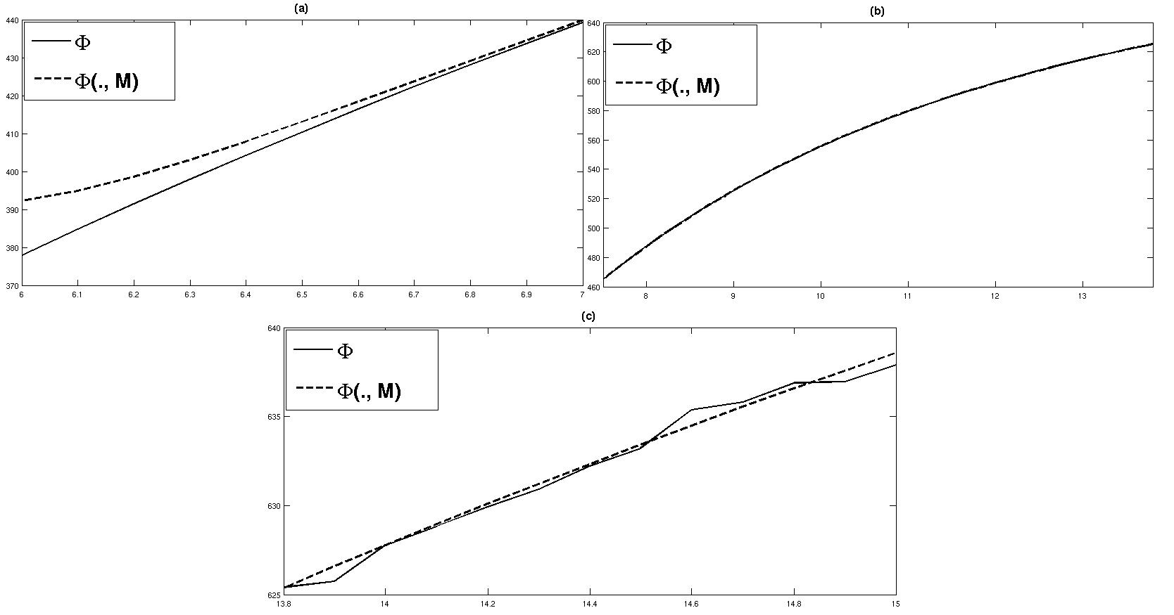
Figure 2: Curves of $\Phi(\beta)$ and $\Phi(\beta,17)$, $p=7$ and $n=4$.

Remark 4.4.

If $\boldsymbol{y}=0$, then LASS0=0 and the mode (20) becomes

$$r(\theta)\|\theta\|_{1}=\frac{\beta(-\beta+\sqrt{\beta^{2}+4(p-1)}}{2}.$$

In Fig.(3) we plot $\beta\in[0.4987,44.5]\to\frac{\beta(-\beta+\sqrt{\beta^{2}+4(p-1)}}{2}$.

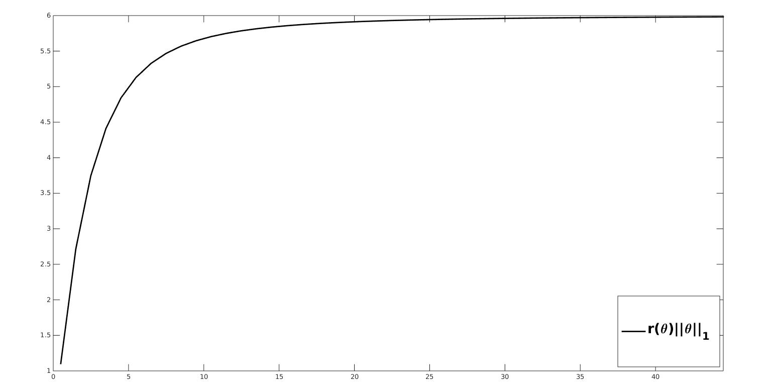
Figure 3: Curve of $r(\theta)\|\theta\|_{1}$, $\beta_{min}:=\frac{1}{\|A\|}=0.4987$, $\beta_{max}=44.5$, $\min(r(\theta)\|\theta\|_{1})=1.1035$, $p=7$ and $n=4$.

The mode of the distribution of $\frac{1}{Z}\exp(-\varphi(r,\theta))drd\theta$ is equal to

$$\arg\min_{r>0,\theta\in S}\varphi(r(\theta),\theta)=(r(\theta^{*}),\theta^{*}).$$

As an illustration we consider $p=7$, $n=4$, $\mathbf{A}\sim\mathcal{B}(\pm\frac{1}{\sqrt{n}})$. We draw uniformly $N=10^{5}$ sample $\theta_{i}\in S$ from the unit sphere $S$. For each $i$, we calculate $\varphi(r(\theta_{i}),\theta_{i})$, and we derive $\theta^{*}$. Notice that $\beta^{*}=\frac{\|\theta^{*}\|_{1}}{\|\mathbf{A}\theta^{*}\|_{2}}=14.0122\approx\beta_{\Phi}$ is nearly equal to the beginning of abnormality of $\Phi$.

Using Formula (5) and Monte Carlo method, we obtain $Z\approx 2.2142$, $Z_{min}\approx 0.0058$ and $Z_{max}\approx 120.3654$. If we draw $N=10^{5}$ vectors using Laplace distribution (3) and calculate the value of $Z$ using Formula (2) and Monte Carlo method, then we obtain $Z\approx 0.0036<Z_{min}$. Hence Monte Carlo method using Formula (5) wins against Monte Carlo method using Formula (2).

5 The case $0\notin LASSO$

If $0\notin LASSO$, then the assertions of Proposition (4.3) are no longer valid. But we are going to show that these assertions becomes valid if we work around LASSO. We consider for $\boldsymbol{l}\in LASSO$,

$$h(\boldsymbol{x}) = -\frac{\|\mathbf{A}(\boldsymbol{x}+\boldsymbol{l})-\boldsymbol{y}\|_{2}^{2}}{2}-\|\boldsymbol{x}+\boldsymbol{l}\|_{1},$$

$$\bar{h}(\boldsymbol{x}) := h(\boldsymbol{x})-h(0),$$

$$f(\boldsymbol{x}) = \exp\Big{(}\bar{h}(\boldsymbol{x})\Big{)}.$$ (21)

Contrary to the map $\boldsymbol{x}\to c(\boldsymbol{x})$, the map $\boldsymbol{x}\to f(\boldsymbol{x})$ attains its supremum at the origin. Observe that

$$c(\boldsymbol{x}) = \frac{f(\boldsymbol{x}-\boldsymbol{l})}{\int_{\mathbb{R}^{p}}f(\boldsymbol{x})d\boldsymbol{x}},$$

$$Z = \exp(h(0))Z_{f}:=\exp(h(0))\int_{\mathbb{R}^{p}}f(\boldsymbol{x})d\boldsymbol{x}.$$

If $\boldsymbol{x}$ is drawn from $c$, then $\boldsymbol{x}-\boldsymbol{l}$ is drawn from $\frac{f}{Z_{f}}$. Moreover

$$Z_{f}=\int_{\mathbb{R}^{p}}f(\boldsymbol{x})d\boldsymbol{x}=\int_{S}J_{p}(\theta,\boldsymbol{l})d\theta,$$ (22)

where

$$J_{p}(\theta,\boldsymbol{l}):=\int_{0}^{+\infty}f(r\theta)r^{p-1}dr.$$ (23)

The map $\boldsymbol{x}\in\mathbb{R}^{p}\to J_{p}^{-\frac{1}{p}}(\boldsymbol{x},\boldsymbol{l}):=\|\boldsymbol{x}\|_{\mathbf{A},\boldsymbol{y},\boldsymbol{l}}$ is nearly a norm (only the eveness is missing). The set

$$K(\mathbf{A},\boldsymbol{y},\boldsymbol{l})=\{\boldsymbol{x}\in\mathbb{R}^{p}:\|\boldsymbol{x}\|_{\mathbf{A},\boldsymbol{y},\boldsymbol{l}}\leq 1\}$$ (24)

is convex, compact and contains the origin. The volume

$$Vol(K(\mathbf{A},\boldsymbol{y},\boldsymbol{l}))=\frac{Z_{f}}{p}.$$

If $\boldsymbol{x}$ is drawn from $c$, then $\boldsymbol{x}-\boldsymbol{l}$ is drawn from $\frac{f}{Z_{f}}$, or equivalently if $\boldsymbol{x}$ is drawn from $\frac{f}{Z_{f}}$, then $\boldsymbol{x}+\boldsymbol{l}$ is drawn from $c$. To draw $\boldsymbol{x}$ from $\frac{f}{Z_{f}}$, we draw $\theta=\frac{\boldsymbol{x}}{\|\boldsymbol{x}\|_{2}}$ uniformely on $S$, and then we draw $\|\boldsymbol{x}\|_{2}$ from

$$\mu_{\theta,\boldsymbol{l}}(r):=\frac{f(r\theta)}{J_{p}(\theta,\boldsymbol{l})}.$$ (25)

We have from [9] Lemma 2.1 and Remarks page 14 the following result.

Proposition 5.1.

1) The function

$$r\in(0,+\infty)\to\varphi(r,\theta,\boldsymbol{l}):=\frac{\|\mathbf{A}(r\theta+\boldsymbol{l})-\boldsymbol{y}\|_{2}^{2}}{2}+\|r\theta+\boldsymbol{l}\|_{1}-(p-1)\ln(r)+h(0)$$

is convex and its unique critical point $r(\theta,\boldsymbol{l})$ is the mode of (25).

2) By denoting $M(\theta,\boldsymbol{l})=\exp\Big{(}-\varphi(r(\theta,\boldsymbol{l}),\theta,\boldsymbol{l})\Big{)}$, we obtain

$$\frac{M(\theta,\boldsymbol{l})r(\theta,\boldsymbol{l})}{p}\leq J_{p}(\theta,\boldsymbol{l})\leq\frac{M(\theta,\boldsymbol{l})r(\theta,\boldsymbol{l})(p-1)!\exp(p-1)}{(p-1)^{p}},$$

and for $q>0$,

$$\int_{qr(\theta,\boldsymbol{l})}\exp(-\varphi(r,\theta,\boldsymbol{l}))dr\leq\frac{p\Gamma(p,(p-1)q)\exp(p-1)}{(p-1)^{p}}\int_{0}^{+\infty}\exp(-\varphi(r,\theta,\boldsymbol{l}))dr.$$

3) We have

$$\frac{|S|\inf_{\theta\in S}M(\theta,\boldsymbol{l})r(\theta,\boldsymbol{l})}{p}\leq Z_{f}\leq\frac{|S|(p-1)!\exp(p-1)}{(p-1)^{p}}\sup_{\theta\in S}M(\theta,\boldsymbol{l})r(\theta,\boldsymbol{l}).$$

4) if $\boldsymbol{x}$ is drawn from the distribution $c$ (1), then $\|\boldsymbol{x}-\boldsymbol{l}\|_{2}\leq qr(\theta,\boldsymbol{l})$ with the probability at least equal to $1-\frac{p\Gamma(p,(p-1)q)\exp(p-1)}{(p-1)^{p}}$.

5.1 Calculation of the mode of (25) and the partition function (23)

Now, we are going to calculate the mode $r(\theta,\boldsymbol{l})$, and the partition function $J_{p}(\theta,\boldsymbol{l})$. The calculations are similar to the case LASSO={0}, but we need new notations. The vector $\boldsymbol{y}_{\boldsymbol{l}}=\boldsymbol{y}-\mathbf{A}\boldsymbol{l}$, $\boldsymbol{s}_{\boldsymbol{l}}=\cos(\theta_{\boldsymbol{l}})$ where $\theta_{\boldsymbol{l}}$ denotes the angle $(\mathbf{A}\theta,\boldsymbol{y}_{\boldsymbol{l}})$, $b_{\boldsymbol{l}}=\|\boldsymbol{y}_{\boldsymbol{l}}\|_{2}s_{\boldsymbol{l}}$. The components of the vector $\boldsymbol{l}\in LASSO$ are denoted by $l_{1}$, …, $l_{p}$. For $\theta\in\mathbb{R}^{p}$, we set

$$S_{0} = \{i\in\{1,\ldots,p\}:\quad\theta_{i}=0\},$$

$$S_{+} = \{i\in\{1,\ldots,p\}:\quad\theta_{i}\neq 0,\quad\theta_{i}l_{i}\geq 0\},$$

$$S_{-} = \{i\in\{1,\ldots,p\}:\quad\theta_{i}\neq 0,\quad\theta_{i}l_{i}<0\}.$$

The cardinality of $S_{-}$ is denoted by $|S_{-}|$, and the order statistic of the sequence $\frac{|l_{i}|}{|\theta_{i}|}$, for $i\in S_{-}$ is denoted by

$$l\theta(0):=0\leq l\theta(1):=\frac{|l|}{|\theta|}(1)\leq\ldots\leq l\theta(|S_{-}|):=\frac{|l|}{|\theta|}(|S_{-}|)\leq l\theta(|S_{-}|+1):=+\infty.$$

Using these new notations, we obtain

$$\|r\theta+\boldsymbol{l}\|_{1}=\sum_{i\in S_{0}}|l_{i}|+\sum_{i\in S_{+}}|\theta_{i}|(r+\frac{l_{i}}{\theta_{i}})+\sum_{i\in S_{-}}|\theta_{i}||r-\frac{|l_{i}|}{|\theta_{i}|}|.$$

If $l\theta(k)\leq r<l\theta(k+1)$, then

$$\|r\theta+\boldsymbol{l}\|_{1}=\|\theta\|_{1,k}r+c_{k},$$

where

$$c_{k}:=\sum_{i\in S_{0}}|l_{i}|+\sum_{i\in S_{+}}|l_{i}|-\sum_{i=0,i\in S_{-}}^{k}|l(i)|+\sum_{i=k+1}^{|S_{-}|}|l(i)|,$$

$$\|\theta\|_{1,k}:=\sum_{i\in S_{+}}|\theta_{i}|+\sum_{i=0,i\in S_{-}}^{k}|\theta(i)|-\sum_{i=k+1,i\in S_{-}}^{|S_{-}|}|\theta(i)|.$$

Observe that $\|\theta\|_{1,|S_{-}|}=\|\theta\|_{1}$, and if $\mathbf{A}\theta=0$ then

$$J_{p}(\theta,\boldsymbol{l})=\exp(-\frac{\|\boldsymbol{y}_{\boldsymbol{l}}\|_{2}^{2}}{2})\sum_{k=0}^{|S_{-}|}\int_{l\theta(k)}^{l\theta(k+1)}\exp(-\|\theta\|_{1,k}r)r^{p-1}dr.$$

Now, we have the following.

Proposition 5.2.

If $\mathbf{A}\theta=0$, then

$$\exp(\frac{\|\boldsymbol{y}_{l}\|_{2}^{2}}{2})J_{p}(\theta,\boldsymbol{l})=\sum_{k\in I_{1}(\theta)}\frac{\exp(-c_{k})\Big{(}(l\theta(k+1))^{p}-(l\theta(k))^{p}\Big{)}}{p}+$$

$$\sum_{k\in I_{2}(\theta)}\frac{\exp(-c_{k})\Big{(}\Gamma(p,l\theta(k))-\Gamma(p,l\theta(k+1))\Big{)}}{\|\theta\|_{1,k}^{p}},$$ (26)

where

$$I_{1}(\theta)=\{k\in\{0,\ldots,|S_{-}|\},\,\,\mbox{such that}\,\,\|\theta\|_{1,k}=0\},$$

$$I_{2}(\theta)=\{k\in\{0,\ldots,|S_{-}|\},\,\,\mbox{such that}\,\,\|\theta\|_{1,k}>0\}.$$

Now, we are going to give the closed form of $J_{p}(\theta,\boldsymbol{l})$ when $\mathbf{A}\theta\neq 0$.

We observe for $l\theta(k)\leq r<l\theta(k+1)$ that

$$\frac{\|r\mathbf{A}\theta+\mathbf{A}\boldsymbol{l}-\boldsymbol{y}\|_{2}^{2}}{2}+\|r\theta+\boldsymbol{l}\|_{1}=\alpha_{k}+\frac{(\|\mathbf{A}\theta\|_{2}r+\beta_{k})^{2}}{2},$$

where

$$\beta_{k}=\frac{\|\theta\|_{1,k}}{\|\mathbf{A}\theta\|_{2}}-b_{\boldsymbol{l}},$$

$$\alpha_{k}=\frac{\|\mathbf{A}\boldsymbol{l}-\boldsymbol{y}\|_{2}^{2}-\beta_{k}^{2}}{2}+c_{k}.$$

Moreover if $k\in I_{1}(\theta)$, then $\beta_{k}=-b_{\boldsymbol{l}}$. Observe also that $\beta_{|S_{-}|}$ is bounded below by $-\|\boldsymbol{y}_{\boldsymbol{l}}\|_{2}\sup(s_{\boldsymbol{l}}:\,\theta\in S)$. It follows that

$$J_{p}(\theta,\boldsymbol{l})=\sum_{k\in I_{1}(\theta)}\exp(-\alpha_{k})J_{p,k}(\theta,\boldsymbol{l})+\sum_{k\in I_{2}(\theta)}\exp(-\alpha_{k})J_{p,k}(\theta,\boldsymbol{l}),$$

where

$$J_{p,k}(\theta,\boldsymbol{l})=\int_{l\theta(k)}^{l\theta(k+1)}\exp(-\frac{(\|\mathbf{A}\theta\|_{2}r+\beta_{k})^{2}}{2})r^{p-1}dr.$$

The calculation of

$$\int_{l\theta(k)}^{l\theta(k+1)}\exp(-\frac{(\|\mathbf{A}\theta\|_{2}r+\beta_{k})^{2}}{2})r^{p-1}dr$$

is similar to Proposition (4.1), and depends on the sign of

$$x_{k}=\|\mathbf{A}\theta\|_{2}l\theta(k)+\beta_{k},$$

$$y_{k}=\|\mathbf{A}\theta\|_{2}l\theta(k+1)+\beta_{k}.$$

Let $k_{0}=\max(k:x_{k}<0)$ and $k_{1}=\min(k:y_{k}>0)$. Observe that $k_{0}+1\geq k_{1}$, and then $y_{k}\leq 0$ for $k<k_{1}\leq k_{0}+1$. It follows for $k<k_{1}$ that

$$J_{p,k}(\theta,\boldsymbol{l})=\frac{1}{\|\mathbf{A}\theta\|_{2}^{p}}\sum_{j=0}^{p-1}2^{\frac{j-1}{2}}\binom{p-1}{j}(-\beta_{k})^{p-1}\Big{(}\gamma(\frac{j+1}{2},\frac{x_{k}^{2}}{2})-\gamma(\frac{j+1}{2},\frac{y_{k}^{2}}{2})\Big{)}.$$

If $k_{1}<k_{0}+1$, then $x_{k_{1}}<0<y_{k_{1}}$ and

$$J_{p,k_{1}}(\theta,\boldsymbol{l})= \frac{1}{\|\mathbf{A}\theta\|_{2}^{p}}\sum_{j=0}^{p-1}2^{\frac{j-1}{2}}\binom{p-1}{j}(-\beta_{k})^{p-1-j}\gamma(\frac{j+1}{2},\frac{y_{k}^{2}}{2})+\frac{1}{\|\mathbf{A}\theta\|_{2}^{p}}$$

$$\sum_{j=0}^{p-1}2^{\frac{j-1}{2}}\binom{p-1}{j}(-\beta_{k})^{p-1}\gamma(\frac{j+1}{2},\frac{x_{k}^{2}}{2}),$$

and for $k>k_{1}$,

$$J_{p,k}(\theta,\boldsymbol{l})= \frac{1}{\|\mathbf{A}\theta\|_{2}^{p}}\sum_{j=0}^{p-1}2^{\frac{j-1}{2}}\binom{p-1}{j}(-\beta_{k})^{p-1}\Big{(}\gamma(\frac{j+1}{2},\frac{y_{k}^{2}}{2})-\gamma(\frac{j+1}{2},\frac{x_{k}^{2}}{2})\Big{)}.$$

If $k_{1}=k_{0}+1$, then $0\leq x_{k_{1}}<y_{k_{1}}$, and for $k\geq k_{1}$,

$$J_{p,k}(\theta,\boldsymbol{l})=\frac{1}{\|\mathbf{A}\theta\|_{2}^{p}}\sum_{j=0}^{p-1}2^{\frac{j-1}{2}}\binom{p-1}{j}(-\beta_{k})^{p-1}\Big{(}\gamma(\frac{j+1}{2},\frac{y_{k}^{2}}{2})-\gamma(\frac{j+1}{2},\frac{x_{k}^{2}}{2})\Big{)}.$$

Now we can show that $J_{p}(\theta,\boldsymbol{l})$ converges to (26) as $\mathbf{A}\theta\to 0$, and we obtain an approximation similar to (19) for $J_{p,k}(\theta,\boldsymbol{l})$ as $\mathbf{A}\theta\to 0$ for each $k\in I_{1}(\theta)$.

6 MCMC diagnosis

Here we take $p=7$, $n=4$, $\mathbf{A}\sim\mathcal{B}(\pm\frac{1}{\sqrt{n}})$ and for simplicity we consider $\boldsymbol{y}=0$. We sample from the distribution $c$ (1) using Hastings-Metropolis algorithm $(\boldsymbol{x}^{(t)})$ and propose the test $\|\boldsymbol{x}^{(t)}\|_{2}\leq qr(\theta^{(t)})$ as a criterion for the convergence. Here $\theta^{(t)}:=\frac{\boldsymbol{x}^{(t)}}{\|\boldsymbol{x}^{(t)}\|_{2}}$. We recall that if $\boldsymbol{x}$ is drawn from the target distribution $c$, then $\|\boldsymbol{x}\|_{2}\leq qr(\theta)$ with the probability at least equal to $P(q,p)$. Table 2 gives the values of the probability $P(q,p)$. Note that for $q\geq 2.5$ the criterion $\|\boldsymbol{x}^{(t)}\|_{2}\leq qr(\theta^{(t)})$ is satisfied with a large probability.

$q$	2	2.5	3	3.5	4	4.5	5
$P(q,p)$	0.6672	0.9446	0.9924	0.9991	0.9999	1.0000	1.0000

Table 2: Values of the probability $P(q,p)$ for $p=7$.

6.1 Independent sampler (IS)

The proposal distribution

$$Q(\boldsymbol{x}_{2},\boldsymbol{x}_{1})=p(\boldsymbol{x}_{2})=\frac{1}{2^{p}}\exp(-\|\boldsymbol{x}_{2}\|_{1}),\quad\forall\,\boldsymbol{x}_{1},\boldsymbol{x}_{2}.$$

The ratio

$$\frac{c(\boldsymbol{x})}{p(\boldsymbol{x})}\leq\frac{2^{p}}{Z},\quad\forall\,\boldsymbol{x}.$$

It’s known that MCMC $(x^{(t)})$ with the target distribution $c$ and the proposal distribution $p$ is uniformly ergodic [11]:

$$\sup_{A\subset\mathcal{B}(\mathbb{R}^{p})}|\mathbb{P}(\boldsymbol{x}^{(t)}\in A\,|\,\boldsymbol{x}^{(0)})-\int_{A}c(\boldsymbol{x})d\boldsymbol{x}|\leq(1-\frac{Z}{2^{p}})^{t}.$$

Here $Z\approx 2.2142$ and then $(1-\frac{Z}{2^{p}})=0.9827$. Figure 4(a) shows respectively the plot of $t\to 5r(\theta^{(t)})$ and $t\to\|\boldsymbol{x}^{(t)}\|_{2}$.

6.2 Random-walk (RW) Metropolis algorithm

We do not know if the target distribution $c$ satisfies the curvature condition in [13] Section 6. Here we propose to analyse the convergence of the Random walk Metropolis algorithm $(\boldsymbol{x}^{(t)})$ using the criterion $\|\boldsymbol{x}^{(t)}\|_{2}\leq qr(\theta^{(t)})$. Figure 4(b) shows respectively the plot of $t\to 5r(\theta^{(t)})$ and $t\to\|\boldsymbol{x}^{(t)}\|_{2}$.

Figures 4 show that contrary to independent sampler algorithm, the random walk (RW) algorithm satisfies early the criterion $\|\boldsymbol{x}^{(t)}\|_{2}\leq 5r(\theta)$. More precisely

• the independent sampler (IS) algorithm begins to satisfy the criterion $\|\boldsymbol{x}^{(t)}\|_{2}\leq 5r(\theta^{(t)})$ at $t=8\times 10^{5}$ iteration.

• The RW algorithm begins to satisfy the criterion $\|\boldsymbol{x}^{(t)}\|_{2}\leq 3.5r(\theta^{(t)})$ at $t=939065$ iteration, but the IS algorithm never satisfies the criterion $\|\boldsymbol{x}^{(t)}\|_{2}\leq 3.5r(\theta^{(t)})$.

We finally compare IS and RW algorithms using the fact that $\int_{\mathbf{R}^{p}}\boldsymbol{x}c(\boldsymbol{x})d\boldsymbol{x}=0$. The best algorithm will furnish the best approximation of the integral $\int_{\mathbf{R}^{p}}\boldsymbol{x}c(\boldsymbol{x})d\boldsymbol{x}$. Table 3 gives the estimators $\frac{1}{N}\sum_{t=1}^{N}x_{IS}^{(t)}\approx\int_{\mathbf{R}^{p}}\boldsymbol{x}c(\boldsymbol{x})d\boldsymbol{x}$ and $\frac{1}{N}\sum_{t=1}^{N}x_{RW}^{(t)}\approx\int_{\mathbf{R}^{p}}\boldsymbol{x}c(\boldsymbol{x})d\boldsymbol{x}$. It follows that $\|\frac{1}{N}\sum_{t=1}^{N}x_{IS}^{(t)}\|_{2}=0.0187$ and $\|\frac{1}{N}\sum_{t=1}^{N}x_{RW}^{(t)}\|_{2}=0.0041$. We conclude that the random walk algorithm wins for both criteria against independent sampler algorithm.

	$x_{1}$	$x_{2}$	$x_{3}$	$x_{4}$	$x_{5}$	$x_{6}$	$x_{7}$
$\hat{x}_{IS}$	-0.0005	-0.0037	0.0016	0.0164	0.0050	0.0021	-0.0058
$\hat{x}_{RW}$	0.0005	-0.0019	-0.0002	0.0012	-0.0005	0.0031	-0.0011

Table 3: $N=10^{6}$, $p=7$, $n=4$ and $q=5$.

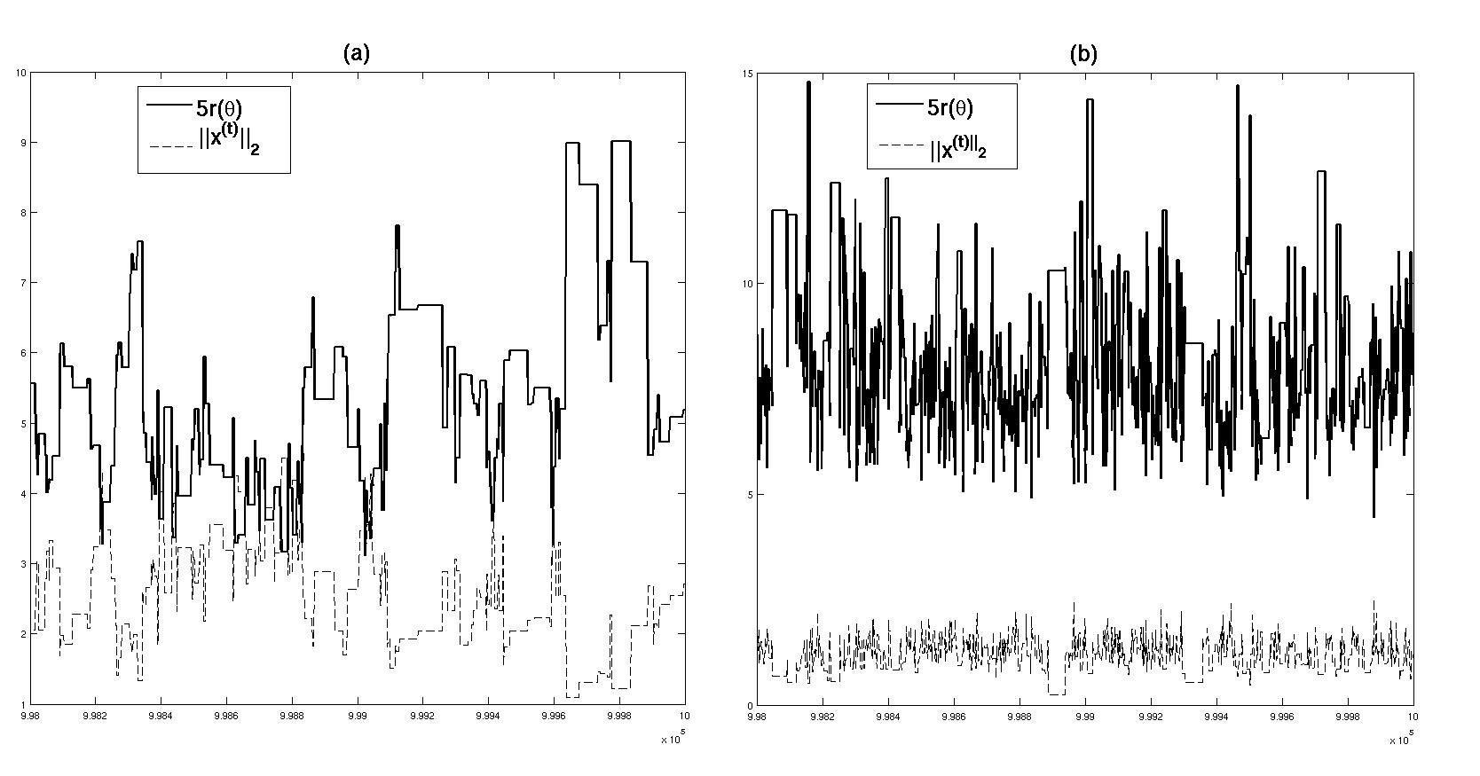
Figure 4: (a): Test of convergence of MCMC algorithm with proposal distribution $p(\boldsymbol{x}_{2})$. (b): Test of convergence of MCMC algorithm with $\mathcal{N}(0,0.5\mathbf{I}_{p})$ proposal distribution. $N=10^{6}$ iterations, $p=7$, $n=4$, $q=5$, $\mathbf{A}\sim\mathcal{B}(\pm\frac{1}{\sqrt{n}})$, $\boldsymbol{y}=0$ and $\boldsymbol{l}=0$.

7 Conclusion

We studied the geometry of bayesian LASSO using polar coordinates and calculated the partition function. We obtained a concentration inequality and derived MCMC convergence diagnosis for the convergence of hasting metropolis algorithm. We showed that the random walk MCMC with the variance 0.5 wins again the independent sampler with the Laplace proposal distribution.

8 References

References

- [1] K. Ball, Logarithmically concave functions and sections of convex sets in , Studia Mathematica, T. LXXXVIII (1988) 70–84.
- [2] A. Beck, M. Teboulle, A Fast Iterative Shrinkage-thresholding Algorithm for linear Inverse Problem, SIAM J. Imaging Sci. (2009) 183–202.
- [3] E.T. Copson, Asymptotic Expansions, Cambridge at the university press (1965).
- [4] S. Chen, D. L. Donoho, M. Saunders. Atomic decomposition by basis pursuit, SIAM J. Sci. Computing, Vol. 20 No. 1 (1998) 33–61.
- [5] I. Daubechies, M. Defrise, C. De Mol, An iterative thresholding algorithm for linear inverse problems with a sparsity constraint, Communications on Pure and Applied Mathematics Vol. LVII (2004), 1413–1457.
- [6] A. Dermoune, D. Ounaissi, N. Rahmania, Oscillation of Metropolis-Hasting and simulated annealing algorithms around penalized least squares estimator, Math. Comput.Simulation (2015).
- [7] B. Efron, T. Hastie, I. Johnstone, R. Tibshirani, Least angle regression, Ann. Statist. 37 (2004) 407–499.
- [8] G. Fort, S. Le Corff, E. Moulines, A. Schreck, A shrinkage-Thresholding Metropolis adjusted Langevin algorithm for Bayesian variable selection, arXiv:1312.5658 (2015).
- [9] B. Klartag, V.D. Milman, Geometry of log-concave functions and measures, Geometriae Dedicata, Volume 112 Issue 1 (2005) 169–182.
- [10] N. Parikh, S. Boyed, Proximal algorithms, Foundation and Trends in Optimization, 1 (3) (2003) 123–231.
- [11] K. Mengersen, R.L Tweedie, Rates of convergence of the Hastings and Metropolis algorithms, The Annals of Statistics (1994) 24:101–121.
- [12] M. Pereyra, Proximal Markov chain Monte Carlo algorithms, Stat. Comput. (2015) 1–16.
- [13] G.0. Roberts, A.L. Tweedie, Geometric convergence and central limit theorems for multidimensional Hastings and Metropolis algorithms, Biometrika 83 1 (1996) 95–110.
- [14] R. Tibshirani, Regression shrinkage and selection via Lasso, Journal of the Royal Statistical Society. Series B. Methodological 58 1 (1996) 267–288.
- [15] R. Tibshirani, The Lasso problem and uniqueness, Electron. J. Stat. 7 (2013) 1456–1490.