The Impact of Molecular Gas on Mass Models of Nearby Galaxies

Abstract

We present CO velocity fields and rotation curves for a sample of nearby galaxies, based on data from the HERACLES survey. We combine our data with literature THINGS, SINGS and KINGFISH results to provide a comprehensive sample of mass models of disk galaxies inclusive of molecular gas. We compare the kinematics of the molecular (CO from HERACLES) and atomic (H i from THINGS) gas distributions to determine the extent to which CO may be used to probe the dynamics in the inner part of galaxies. In general, we find good agreement between the CO and H i kinematics with small differences in the inner part of some galaxies. We add the contribution of the molecular gas to the mass models in our galaxies by using two different conversion factors $\mathrm{\alpha_{CO}}$ to convert CO luminosity to molecular gas mass surface density - the constant Milky Way value and the radially varying profiles determined in recent work based on THINGS, HERACLES and KINGFISH data. We study the relative effect that the addition of the molecular gas has upon the halo rotation curves for Navarro-Frenk-White (NFW) and the observationally motivated pseudo-isothermal halos. The contribution of the molecular gas varies for galaxies in our sample — for those galaxies where there is a substantial molecular gas content, using different values of $\mathrm{\alpha_{CO}}$ can result in significant differences to the relative contribution of the molecular gas and, hence, the shape of the dark matter halo rotation curves in the central regions of galaxies.

1. Introduction

Rotation curves of nearby galaxies provide strong evidence for the existence of dark matter (see Sofue & Rubin 2001). They were first obtained using optical spectroscopy (Rubin & Ford 1970) and soon thereafter radio observations in the 21-cm line of neutral hydrogen (H i) revealed that rotation curves remain flat over many multiples of the optical radius (Warner et al. 1973; van der Kruit & Bosma 1978; Bosma 1978; Bosma et al. 1981; Bosma 1981a, b).

Studies of the rotation curves of the inner parts of galaxies are important in discerning competing models of dark matter. The cuspy dark matter density profiles predicted from $\Lambda$CDM simulations require steeply rising rotation curves (Navarro et al. 1997), while pseudo-isothermal halos representing a cored potential are seen observationally (de Blok 2010). These halo models show the largest differences in the centres of galaxies. It is hence essential that we form a better understanding of the kinematics in the inner regions of galaxies. The central parts of spiral galaxies, especially early-types, tend to have little or no H i, making it difficult to determine the central dynamics from observations of the H i alone. However, molecular gas is typically concentrated in the centres of galaxies, and CO is an abundant tracer of the molecular gas ($\mathrm{H_{2}}$) content of galaxies.

Compared to H i, CO is more easily observable at higher redshifts (Carilli & Walter 2013), which makes CO an alternative tracer of the dynamics in studies of the Tully-Fisher relation (TFR).

The Five Colleges Radio Astronomy Observatory (FCRAO) survey (Young et al. 1995), the Berkeley Illinois Maryland Association Survey of Nearby Galaxies (BIMA-SONG, Helfer et al. 2003) and the recent survey by Kuno et al. (2007) are some of the most comprehensive surveys of the CO content of spiral galaxies. More recently, the ATLAS-3D (Young et al. 2011) survey carried out observations of early type galaxies, and the NUclei of GAlaxies collaboration (NUGA, Garcia-Burillo et al. 2003; Combes et al. 2004; Krips et al. 2005, for example) studied the molecular chemistry and dynamics of the inner parts of nearby active galaxies.

Pioneering studies of the kinematics of spiral galaxies with CO observations were presented in Sofue (1996, 1997) and Sofue et al. (1999). More recently, concerted efforts have been made to map a representative sample of nearby galaxies in H i and CO with The H i Nearby Galaxy Survey (THINGS, Walter et al. 2008) and The HERA CO Line Extragalactic Survey (HERACLES, Leroy et al. 2009), respectively. These surveys, in combination with ancillary data at other wavelengths, provide a comprehensive view of the gaseous ISM of nearby galaxies.

In this paper, we study the kinematics of the CO in a sample of the THINGS galaxies using the HERACLES data, and we extend the analysis of the dynamics performed in de Blok et al. (2008) (hereafter dB08), by including the contribution of the molecular gas. We compare our results to the analysis of the H i kinematics, aiming to address the following questions: How similar are the kinematics of the CO and the H i? How does the CO-TFR compare with the H i-TFR for the same sample of galaxies? What is the effect of adding molecular gas on the derived mass model parameters?

This paper is organized as follows: in Section 2 we describe the CO and H i data; in Section 3 we describe how we compute the velocity fields. The rotation curve derivations are described in Section 4. In Section 5 we present rotation curves. In Section 6 we present the TFR. In Section 7 we outline the motivation and the method used in constructing mass models, and we present the results of the mass modelling in Section 8. Finally, we summarize our study of the dynamics of the galaxies in our sample in Section 9.

2. The Data

Table 1The THINGS-Model geometrical parameters.

Name	Morphology	$\alpha(2000)$	$\delta(2000)$	$D$	$\mathrm{log}(\frac{D_{25}}{0\farcm 1}$)	$V_{\mathrm{sys}}$	$\langle i\rangle$	$\langle pa\rangle$
		$(\mathrm{{}^{h}\,{}^{m}\,{}^{s}})$	$(\mathrm{{}^{{}^{\circ}}\,{}^{{}^{\prime}}\,{}^{{}^{\prime\prime}}})$	($\mathrm{Mpc}$)		($\,\mathrm{km\,s^{-1}}$)	(∘)	(∘)
(1)	(2)	(3)	(4)	(5)	(6)	(7)	(8)	(9)
NGC 0925	SABd	$02\,27\,16.5$	$+33\,34\,43.5$	$9.2$	$2.0$	$546.3$	$66.0$	$286.6$
NGC 2403	SABcd	$07\,36\,51.1$	$+65\,36\,02.9$	$3.2$	$2.2$	$132.8$	$62.9$	$123.7$
NGC 2841	SAb	$09\,22\,02.6$	$+50\,58\,35.4$	$14.1$	$1.8$	$633.7$	$73.7$	$152.6$
NGC 2903	SABbc	$09\,32\,10.1$	$+21\,30\,04.3$	$8.9$	$2.0$	$555.6$	$65.2$	$204.3$
NGC 2976	SAc pec	$09\,47\,15.3$	$+67\,55\,00.0$	$3.6$	$1.8$	$1.1$	$64.5$	$334.5$
NGC 3198	SBc	$10\,19\,55.0$	$+45\,32\,58.9$	$13.8$	$1.8$	$660.7$	$71.5$	$215.0$
NGC 3521	SABbc	$11\,05\,48.6$	$-00\,02\,09.2$	$10.7$	$1.9$	$803.5$	$72.7$	$339.8$
NGC 3627	SABb	$11\,20\,14.9$	$+12\,59\,29.5$	$9.3$	$2.0$	$708.2$	$61.8$	$173.0$
NGC 4736	SAab	$12\,50\,53.0$	$+41\,07\,13.2$	$4.7$	$1.8$	$306.7$	$41.4$	$296.1$
NGC 5055	SAbc	$13\,15\,49.2$	$+42\,01\,45.3$	$10.1$	$2.0$	$496.8$	$59.0$	$101.8$
NGC 6946	SABcd	$20\,34\,52.2$	$+60\,09\,14.4$	$5.9$	$2.0$	$43.7$	$32.6$	$242.7$
NGC 7331	SAb	$23\,57\,49.7$	$-32\,35\,27.9$	$3.9$	$1.9$	$818.3$	$75.8$	$167.7$

In this work we use data from the THINGS and HERACLES surveys. Both surveys have similar spatial and velocity resolution (HERACLES: $13^{\prime\prime}$ and $2.6\,\mathrm{km\,s^{-1}}$, THINGS: $\sim 10^{\prime\prime}$ and a velocity resolution $\leq\,5.2\,\mathrm{km\,s^{-1}}$).

The observational details of the HERACLES survey are described in Leroy et al. (2009). The survey used the IRAM 30-m telescope to map the CO $J=2\rightarrow 1$ transition (rest frequency $\sim 230.538$ GHz) in a sample of nearby galaxies.

We focus on a subset of the HERACLES galaxies for our analysis. These galaxies were selected as follows: 34 galaxies were observed as part of the THINGS survey. dB08 performed an analysis of the dynamics on 19 of the galaxies with intermediate inclinations (i.e., neither face- nor edge-on). Of the 19 dB08 galaxies, the 12 that have molecular gas detected in them form our sample. The general properties of these galaxies are summarized in Table 1. These properties are taken from the THINGS papers: general properties follow from Walter et al. (2008), centre positions follow from Trachternach et al. (2008) and kinematical data (e.g., inclination) follow from dB08.

We use the THINGS date cubes derived using natural weighting and the associated data products.

The velocity resolution of HERACLES was $2.6\,\mathrm{km\,s^{-1}}$ and Hanning smoothing was used to increase the signal-to-noise for various galaxies. This resulted in effective velocity resolutions of $5.2\,\mathrm{km\,s^{-1}}$ for NGC 925, NGC 2403, NGC 2903, NGC 2976, NGC 3198, NGC 3627, NGC 4736, NGC 5055, NGC 6946 and $10.4\,\mathrm{km\,s^{-1}}$ for NGC 2841, NGC 3521 and NGC 7331. In all cases the velocity smoothing makes a negligible difference to the emission line profile and the data products derived from the cubes. The spatial resolution in these cubes is $13^{\prime\prime}$. We only consider channels within the velocity range bound by the H i emission as estimated using the H i position-velocity pV diagram. We then masked the cubes using the masks determined in Leroy et al. (2009) and recalculated the average noise-per-channel in regions which did not contain any CO emission. These values are slightly different from those derived in Leroy et al. (2009), since the noise is a function of frequency and therefore the value depends slightly on the channels chosen. In Table 2 we present the noise values used in this work, compared with those from Leroy et al. (2009). The masking left a few anomalous pixels corresponding to noise-peaks, which we carefully removed with a round of manual masking. We used these cubes to derive the CO global profiles which we compare with the H i profiles as published in Walter et al. (2008). In Figure 1 we plot the H i and CO global profiles for all the THINGS galaxies detected by HERACLES, i.e., also including the galaxies not in our sample. In Figure 2 we plot a comparison of the CO and H i linewidths at the $20\%$ and $50\%$ levels respectively. Some profile shapes lead to ambiguous definitions of $W_{50}$, e.g., NGC 2903 and NGC 2976. For these galaxies we choose the largest value. Figure 2 shows that the CO linewidths are lower than the H i linewidths, on average. This is because the distribution of the CO does not extend as far as the H i and does not trace the full intrinsic velocity-width of a galaxy, (see, e.g., de Blok & Walter 2014).

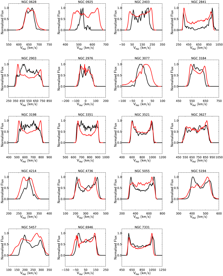
Figure 1.— CO (black) and H i (red) emission line global profiles from the HERACLES and THINGS surveys respectively. The profiles are normalized by their peak fluxes.

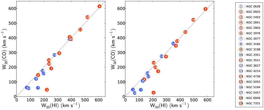
Figure 2.— A comparison of the CO and H i linewidths at $20\%$ and $50\%$ of maximum intensity, respectively. The left subplot shows the $W_{20}$ comparison and the right subplot shows the $W_{50}$ comparison. The line indicates a unity ratio. The number in each circle corresponds to a galaxy in our sample, as shown in the legend on the right. The colour of each circle corresponds to whether or not the galaxy is part of the sub-sample for which we will perform a kinematical analysis in this paper — galaxies in our sample are coloured in red symbols; the others are plotted blue. The typical uncertainties in the linewidths are approximately half the channel width of $2.6\,\mathrm{km\,s^{-1}}$. The corresponding error bars, if plotted on this scale, will be smaller than the markers.

Table 2Noise in H i and CO data cubes.

Galaxy	$\sigma_{\mathrm{CO}}$	$\sigma_{{\mathrm{CO^{\prime}}}}$	$\sigma_{{\rm{H\sc{I}}}}$
	(${\rm{mK}}$)	(${\rm{mK}}$)	${\mathrm{(mJy\,beam^{-1}})}$
(1)	(2)	(3)	(4)
NGC 0925	22	20	0.57
NGC 2403	$\ldots$	24	0.38
NGC 2841	44	26	0.65
NGC 2903	23	24	0.41
NGC 2976	21	24	0.36
NGC 3198	17	20	0.33
NGC 3521	22	25	0.40
NGC 3627	$\ldots$	27	0.43
NGC 4763	23	23	0.33
NGC 5055	24	34	0.36
NGC 6946	25	29	0.55
NGC 7331	20	21	0.44

3. Velocity Fields

Returning to the rotation curve sample listed in Table 1 — we use the Hanning-smoothed HERACLES cubes to derive velocity fields for the CO emission. There are two commonly used methods to compute velocity fields from image cubes - calculating the Intensity Weighted Mean (IWM) of profile values and fitting functions (e.g., Gaussians) to the profiles in an image cube. For asymmetric profiles the IWM of a profile can be affected by the presence of tails to higher and lower velocities, and hence does not always provide an accurate representation of the gas velocity. We therefore fit Gauss-Hermite polynomials of order 3 to the profiles along each pixel in the image cubes, using the prescription described in van der Marel & Franx (1993), and as in dB08. This allows us to account for asymmetry in the profiles, hence determining a more accurate estimate of the gas bulk velocity. We denote these Gauss-Hermite velocity fields as “$\mathrm{Her_{3}}$ velocity fields”. We use the GIPSY (Groningen Image Processing SYstem, van der Hulst et al. 1992) task XGAUFIT to compute the $\mathrm{Her_{3}}$ velocity fields from the masked data as described above.

We also compute the IWM velocity fields from the masked HERACLES cubes using the GIPSY task MOMENTS. In the derivation of both the IWM and $\mathrm{Her_{3}}$ velocity fields we reject values less than $3\,\sigma_{\mathrm{CO^{\prime}}}$ where $\sigma_{\mathrm{CO^{\prime}}}$ is the average noise-per-channel indicated in Table 2.

In the appendix we plot the IWM and $\mathrm{Her_{3}}$ velocity fields for each galaxy in our sample, as well as the H i velocity fields calculated in dB08.

4. Rotation Curve Derivation

We use the $\mathrm{Her_{3}}$ velocity fields to calculate the rotation curves using a tilted-ring model (Begeman 1989). In the tilted-ring analysis, a two-dimensional velocity field of a galaxy is decomposed into a set of rings, each with an associated set of parameters: the systemic velocity $V_{\mathrm{sys}}$, the centre position $(x_{0},y_{0})$ on the sky, the inclination angle $i$ defined as the angle between the normal to the plane of the galaxy and the line-of-sight, the position angle $pa$ of the major-axis on the sky, and the circular velocity $V_{c}$. A tilted-ring model is thus characterized by a set of parameters $(x_{o},y_{o},V_{\mathrm{sys}},i,pa,V_{\mathrm{c}})$ for each ring and can therefore vary with radius.

Assuming the gas moves in purely circular orbits, the observed line-of-sight velocity $V$ at an arbitrary position $(x,y)$ on a ring of radius $r$ can be expressed as:

$$V(x,y)=V_{\mathrm{sys}}+V_{\mathrm{c}}(r)\sin(i)\cos(\theta)$$ (1)

where $\theta$ is the azimuthal or position angle with respect to the receding major-axis, measured in the plane of the galaxy. It is related to the position angle of the major-axis in the plane of the sky by the following relations:

$$\cos(\theta)=\frac{-(x-x_{0})\sin(pa)+(y-y_{0})\cos(pa)}{r}$$ (2)

$$\sin(\theta)=\frac{-(x-x_{0})\cos(pa)-(y-y_{0})\sin(pa)}{r\cos(i)}$$ (3)

For each ring, the parameters are solved using a least squares algorithm to obtain an optimal fit.

We use the GIPSY task ROTCUR to calculate rotation curves from the $\mathrm{Her_{3}}$ velocity fields, solving for kinematic parameters along rings which are spaced by half-a-beamwidth, i.e., Nyquist sampled. We use the filling-factor for each ring to determine whether to include it in the tilted-ring fit. We define the filling factor as the ratio of the area with significant signal and the total area of each ring. A filling-factor of $5\%$ is used as a cutoff, since solving for parameters on rings with lower filling-factors does not lead to useful results.

We calculate two different types of rotation curves. Firstly, we use the tilted-ring model parameters as determined in dB08: we fix them and simply apply them to the CO velocity field solving for $V_{\mathrm{c}}$ only. We refer to these models as the THINGS models (TM). For galaxies where there is a central depression in the H i distribution and therefore no corresponding values (e.g., NGC 7331), we extrapolate the tilted-ring parameters from the innermost point by assuming that these parameters remain constant.

Secondly, we determine the tilted-ring model for a subset of the galaxies in our sample for which the CO coverage is sufficiently good to constrain a separate tilted-ring model. We refer to these models as the HERACLES models (HM). For the HM we use an iterative method, where we use TM as a starting point. We then alternate between solving for $(V_{\mathrm{sys}},x,y)$ and $(pa,i)$, each time holding the other set of parameters fixed. We repeat this until the model parameters converge. We assume that the centre and the systemic velocity of the galaxy do not vary from ring to ring. We smooth radially varying position-angle and inclination values using a five-point boxcar smoothing algorithm to suppress small scale variations. After the parameters have converged, we fix them and solve for $V_{\mathrm{c}}$ alone.

To estimate the uncertainties along each ring we use the same prescription as dB08. The errors are defined as the quadratic sum of the dispersion in velocity values along each tilted-ring and the uncertainty due to the approaching and receding side of the galaxy, which is defined as a quarter of the difference. The rotation curves from the approaching and receding sides are calculated by running ROTCUR on the corresponding half of the galaxy only. In general, we find the dispersion in velocities to be the larger contributor to the total error.

For the galaxies in the dB08 sample HMs could be derived for NGC 2403, NGC 2976, NGC 3198, NGC 3521, NGC 5055 and NGC 7331. For the other galaxies there is either too little detected CO emission to constrain the models (for NGC 925 and NGC 2841), or the low inclinations prohibits the independent constraint of the kinematic parameters (for NGC 4736 and NGC 6946). For NGC 2903 the effect of the strong bar makes it difficult to solve for a tilted-ring model since the CO velocities are heavily influenced by bar streaming motions. NGC 3627 is part of the Leo Triplet and the observations show signs of tidal interaction with the neighbouring galaxies. For these six galaxies we therefore only calculate a TM.

4.1. Beam Smearing

The high resolution of HERACLES allows us to study the distribution of the CO in great detail. However, despite the relatively high spatial resolution, the finite beam size can still lead to beam smearing effects near the central parts of the galaxies. This would affect the derived rotation curve and becomes more significant for galaxies at a high inclination. To quantify the possible effect that beam smearing may have on the derived rotation curves, we did a simple study using model galaxies. We used the GIPSY task GALMOD to construct model galaxies with a constant inclination of $70^{\circ}$, a Gaussian scale height of $100\,\mathrm{pc}$, a constant column density across the disk of $2\times 10^{21}\,\mathrm{cm}^{-2}$ and a velocity dispersion of $8\,\mathrm{km\,s^{-1}}$. This model is very similar to that presented in dB08.

The rotation curve used as input to GALMOD rises linearly to a maximum of $250\,\mathrm{km\,s^{-1}}$, and stays constant at this maximum for the rest of the disk. We used four different rotation curves to quantify the effect of beam smearing. We varied the radius at which the rotation curve reached the maximum velocity, using radii of $6.5^{\prime\prime}$, $13^{\prime\prime}$, $26^{\prime\prime}$ and $60^{\prime\prime}$ respectively. With these input rotation curves we can study how the effect of beam smearing changes when the rotation curve reaches a maximum within a resolution element, to when the rotation curve reaches its maximum at larger radii.

GALMOD produces model data cubes given these galaxy parameters. We smoothed these data cubes to the $13^{\prime\prime}$ resolution of HERACLES, and computed the $\mathrm{Her_{3}}$ velocity fields and rotation curves from the “observed” galaxy cubes. The results are presented in Figure 3.

This shows that while beam smearing has a large effect on the observed rotation curve when the input rotation curve rises to a maximum within a resolution element, it becomes negligible when the input rotation curve rises to a maximum at radii larger than two resolution elements, as shown in Figure 3. This is the case for all the galaxies in our sample. Furthermore, the inclination of the galaxies in our sample are less than $70^{\circ}$, except for NGC 7331. Beam smearing is thus expected to play only a negligible here.

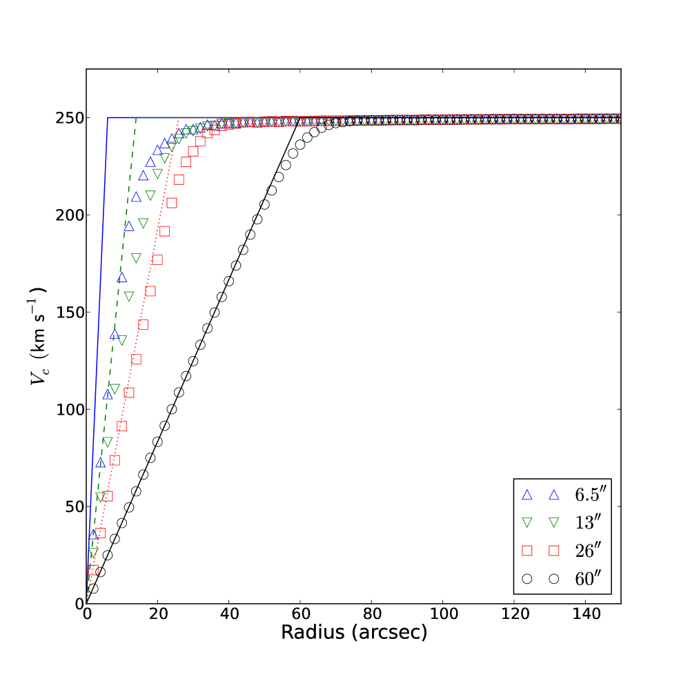
Figure 3.— Comparison of model rotation curves with resultant observed rotation curves. The blue-solid, green-dashed, red-dotted and black-solid lines represent input rotation curves with a linear rise to a maximum velocity of $250\,\mathrm{km\,s^{-1}}$ within $6.5^{\prime\prime}$, $13^{\prime\prime}$, $26^{\prime\prime}$ and $60^{\prime\prime}$ respectively. The blue upward-triangles, green downward-facing triangles, red squares and black circles represent the observed output rotation curves derived from each of the associated input rotation curves.

5. Results and Discussion - Kinematics

The rotation curves are plotted in Figures 4 (TM) and 5 (HM) respectively. The corresponding HM tilted-ring parameters for NGC 2403, NGC 2976, NGC 3198, NGC 3521, NGC 5055 and NGC 7331 are presented in Table 4. In the appendix we present our full results: H i and CO velocity fields (IWM and $\mathrm{Her_{3}}$); CO integrated surface brightness contours overlaid on the Spitzer Infrared Nearby Galaxy Survey (Kennicutt et al. 2003, SINGS) 3.6$\mu$m images, pV major- and minor-axis diagrams and H i and CO TM/HM rotation curves. For each of the tilted-ring models considered in this work we compute an associated model velocity field and we calculate the residuals by taking the difference between the model and observed velocity fields. As the residuals generally have a Gaussian distribution (except where there are major non-axisymmetric features, such as bars), we fit a Gaussian function to the normalised histogram of the residuals to estimate the mean $\mu$ and the standard deviation $\sigma$. These values are presented in Table 3. In the appendix we also provide a brief description of the rotation curves for each galaxy. We also fit a functional form to the CO rotation curves presented in this work, which is also presented in the appendix. Using such a functional form allows for the computation of the derivative of the rotation curve which is important in determining the star formation threshold, for example (see, e.g., Leroy et al. 2008).

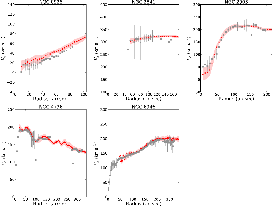
Figure 4.— CO and H i rotation curves for NGC 925, NGC 2841, NGC 2903, NGC 3627, NGC 4736 and NGC 6946. The H i rotation curves from dB08 are plotted as filled red circles; the associated errors are plotted as a filled red region. The CO rotation curves are computed using the TM, i.e., using the tilted-ring model parameters based on the H i data, and are plotted as filled grey squares with errorbars.

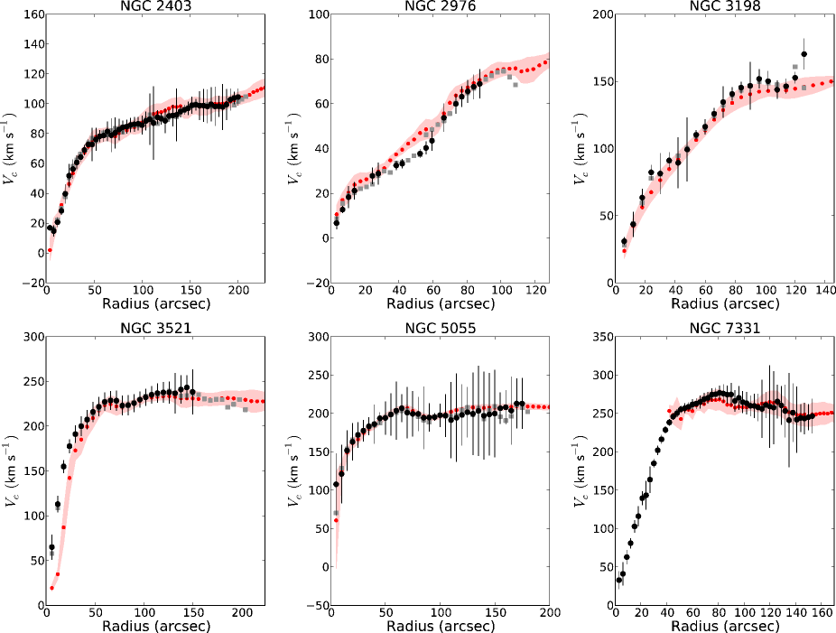
Figure 5.— CO and H i rotation curves for NGC 2403, NGC 2976, NGC 3198, NGC 3521, NGC 5055 and NGC 7331. The H i rotation curves from dB08 are plotted as filled red circles; the associated errors are plotted as a filled red region. The CO rotation curves are computed using the THINGS-Model (TM) and the independently determined HERACLES-Model (HM). The TM rotation curves are plotted as filled grey squares, HM rotation curves are plotted as filled black circles with errorbars.

Table 3Statistics from the tilted-ring model fits to the $\mathrm{Her_{3}}$ velocity fields derived from the HERACLES data.

Name	$\sigma_{\mathrm{TM}}$	$\mu_{\mathrm{TM}}$	$\sigma_{\mathrm{HM}}$	$\mu_{\mathrm{HM}}$
	$(\,\mathrm{km\,s^{-1}})$	$(\,\mathrm{km\,s^{-1}})$	$(\,\mathrm{km\,s^{-1}})$	$(\,\mathrm{km\,s^{-1}})$
NGC 0925	5.26	2.46	$\ldots$	$\ldots$
NGC 2403	5.51	0.03	5.72	-1.47
NGC 2841	7.02	1.61	$\ldots$	$\ldots$
NGC 2903	12.7	-2.06	$\ldots$	$\ldots$
NGC 2976	3.85	-3.44	2.84	0.66
NGC 3198	4.38	-3.04	4.93	-1.27
NGC 3521	7.92	0.57	5.45	-1.58
NGC 3627	13.3	-2.57	$\ldots$	$\ldots$
NGC 4736	5.19	1.42	$\ldots$	$\ldots$
NGC 5055	6.31	-2.40	6.09	-3.34
NGC 6946	5.83	-1.41	$\ldots$	$\ldots$
NGC 7331	14.7	-3.37	11.96	-1.17

Table 4The HERACLES-Model tilted-ring parameters

Name	$\alpha\,(2000)$	$\delta(\,2000)$	$V_{\mathrm{sys}}$	$\langle i\rangle$	$\langle pa\rangle$
	$(\mathrm{{}^{h}\,{}^{m}\,{}^{s}})$	$(\mathrm{{}^{{}^{\circ}}\,{}^{{}^{\prime}}\,{}^{{}^{\prime\prime}}})$	($\,\mathrm{km\,s^{-1}}$)	(∘)	$(^{\circ})$
NGC 2403	07 37 15.8	+65 30 17.1	132.9	59.2	120.2
NGC 2976	09 47 26.4	+67 51 04.2	1.1	65.7	338.8
NGC 3198	10 19 42.7	+45 36 40.3	659.9	68.3	211.1
NGC 3521	11 06 01.3	+00 02 25.7	802.3	67.4	120.0
NGC 5055	13 15 15.7	+42 04 16.8	497.0	63.6	98.5
NGC 7331	22 37 05.3	+34 30 07.7	822.8	72.0	167.1

For NGC 2403, NGC 2841, NGC 3627, NGC 4736, NGC 6946 and NGC 7331 there is excellent agreement between the H i and CO rotation curves. For NGC 925, NGC 2903, NGC 2976, NGC 3198, NGC 3521 and NGC 5055 there are some differences which can be explained by the presence of bars and the lopsided emission of the CO in comparison to the H i. For NGC 4736, NGC 6946 and NGC 7331 the CO rotation curves also covers the inner part of the galaxy not traced by the H i emission. We conclude that CO is a good tracer of the rotation curve in the inner part of galaxies. For NGC 2903 there is a clear indication of the effect of the bar on the velocity field. In the following sub-section we present a brief analysis of the non-circular motions in NGC 2903.

Detailed comments about the kinematics and rotation curves for each galaxy are presented the Appendix.

5.1. Non-circular Motions in NGC 2903

NGC 2903 hosts a strong bar, which is closely aligned to the major axis of the disk. The inner part of the H i distribution is strongly affected by the non-circular streaming motions due to the bar, as noted in Trachternach et al. (2008). They present an analysis of non-circular motions in the THINGS galaxies and estimate the amplitude of the higher order coefficients in a Fourier series description of the velocity field. These coefficients can be interpreted as perturbations due to physical effects, such as radial motions or streaming motions - as due to a bar, for example. While the amplitudes of the non-circular motions are estimated by Trachternach et al. (2008), they do not discuss how these might affect the circular rotation curve. Spekkens & Sellwood (2007) use a Fourier series expansion to describe the radial and tangential components of non-circular motions as higher order perturbations, and explicitly correct for these effects on the rotation curve. This formalism was coded into the software tool VELFIT. Sellwood & Sánchez (2010) used VELFIT to derive a model velocity field and corrected rotation curve using a bar-like ($m=2$ in the Fourier expansion) perturbation to the THINGS H i velocity field and the BH$\alpha$Bar $\mathrm{H\alpha}$ velocity field (Hernandez et al. 2005) for NGC 2903. We used an updated version of the VELFIT tool called DISKFIT (Kuzio de Naray et al. 2012; Sellwood & Spekkens 2015) to model the HERACLES velocity field of NGC 2903.

Using the CO total intensity image and velocity field we estimated the radial extent of the bar to be approximately $56^{\prime\prime}$. We solve for a bar-like perturbation corresponding to the $m=2$ mode within $56^{\prime\prime}$ (in addition to circular rotation) and we assume that the gas is regularly rotating at larger radii. We also solve for the systemic velocity, disk position angle $\phi^{\prime}_{\mathrm{d}}$, inclination angle and central position. The resultant velocity field is further characterized by the bar position angle in the disk-plane (denoted as $\phi_{\mathrm{d}}$) and the sky-plane (denoted as $\phi^{\prime}_{\mathrm{b}}$).

Because of its higher signal-to-noise, we used the IWM velocity field to solve for the non-circular motions. Tests show the output rotation curves when using either the IWM and $\mathrm{Her_{3}}$ velocity fields are identical.

The resulting best fit parameters and the associated uncertainties from our DISKFIT run are presented in Table 5, along with the values presented in Sellwood & Sánchez (2010). We plot the rotation curve, $V_{\mathrm{t}}$, and the tangential and radial components of the $m=2$ mode, denoted as $V_{\mathrm{2,t}}$ and $V_{\mathrm{2,r}}$ respectively, in Figure 6.

We note a relatively good agreement between our parameters and those presented in Sellwood & Sánchez (2010). The best fit inclination and disk position angle are consistent with the THINGS values, and the systemic velocity is slightly higher than the THINGS value and the Sellwood & Sánchez (2010) values. The best fit central position is identical to the coordinates presented in Table 1. The bar position angles are different from the values in Sellwood & Sánchez (2010), but agree within the uncertainties. Sellwood & Sánchez (2010) noted that the close alignment of the bar axis with the major axis of the disk made the modelling of the bar perturbation difficult and, therefore, the bar position angles solved for in this work still have a large uncertainty. We will not consider the bar in our further models.

Table 5DISKFIT results for NGC 2903.

Parameter	HERACLES	THINGS	BH$\alpha$Bar
$V_{\mathrm{sys}}\,(\,\mathrm{km\,s^{-1}})$	$558.8\pm 1.2$	$549.9\pm 0.3$	$554.1\pm 0.5$
$i\ (^{\circ})$	$64.5\pm 4.8$	$64.0\pm 1.0$	$66.0\pm 3$
$\phi^{\prime}_{\mathrm{d}}\ (^{\circ})$	$206.1\pm 1.9$	$201.5\pm 0.5$	$204.0\pm 1$
$\phi_{\mathrm{b}}\ (^{\circ})$	$17\pm 8$	$6\pm 14$	$-12\pm 8$
$\phi^{\prime}_{\mathrm{b}}\ (^{\circ})$	$214\pm 7$	$204\pm 6$	$199\pm 4$

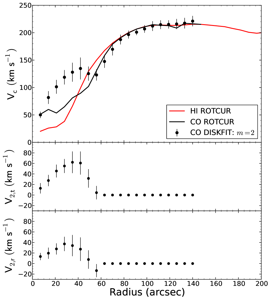
Figure 6.— DISKFIT model rotation curves for NGC 2903 for an $m=2$ perturbation. In the top panel we plot the observed rotation curves from the THINGS data (red-line) and the HERACLES data (black-line) using ROTCUR. In this model we solve and correct for the $m=2$ modes in the velocity field by assuming that the non-circular motions are dominant within $56^{\prime\prime}$. The black filled circles with errorbars correspond to the DISKFIT rotation curve. In the second panel we plot the tangential component for the $m=2$ mode, denoted as $V_{\mathrm{2,t}}$. In the third panel we plot the radial component for the $m=2$ mode, denoted as $V_{\mathrm{2,r}}$.

6. The Tully-Fisher Relation

As in Section 2, we again consider all galaxies overlapping in the THINGS/HERACLES sample detected CO. We present a comparison of the CO and H i TFRs for the galaxies. Since the galaxies studied here are comparatively massive, we restrict our study to the classical TFR and not the baryonic TFR (McGaugh et al. 2000). de Blok & Walter (2014) demonstrated how the distribution of the gas tracer leads to different global profiles and hence different TFRs even for identical rotation curves. In general, the CO has a compact distribution, while the more constant H i surface density extends to beyond the optical radius of the galaxy. This can also be seen in the radial mass surface densities of the molecular gas and the H i, as shown in Leroy et al. (2008) - the shape of the $\mathrm{H_{2}}$ distribution closely follows the exponential stellar distribution, while the H i distribution remains relatively constant over a large range of radii. Here we use the CO linewidths as plotted in Figure 1 to show the effect of these differences on the TFR.

Many profiles are double-horned with steep sides, which is indicative of massive spiral galaxies. We exclude two profiles for two galaxies where the linewidths cannot be used as a proxy for the maximum rotational velocity — NGC 925 and NGC 3077. For NGC 925 the emission is one-sided, and for NGC 3077 the gas is tidally disturbed.

We make an inclination correction to the CO and H i global profiles. For the H i profiles we simply use the THINGS inclinations presented in Walter et al. (2008), except for NGC 5194, for which we use the improved inclination from Colombo et al. (2014). For the CO profiles we also use these inclinations except for the galaxies for which we have HM models. For these galaxies we use the average inclinations given in Table 4. The inclination corrected rotation velocities are denoted by $V^{i}$, assuming that the linewidths can be used as a proxy for the rotational velocity through $V^{i}=\frac{W^{i}}{2}$.

Verheijen (2001) calculated the TFR for galaxies in the Ursa Major Cluster of galaxies, and found a reduced scatter in the $K^{\prime}$-band. We therefore calculate the infrared TFR with data from the Spitzer Survey of Stellar Structure in Galaxies (S⁴G, Sheth et al. 2010), and compare this with the TFR presented in Sorce et al. (2014).

Using the distances from Walter et al. (2008) we convert the $3.6\mu\mathrm{m}$ apparent magnitudes from S⁴G to absolute magnitudes. NGC 2403, NGC 6946 and NGC 7331 were not part of the S⁴G sample. We therefore exclude them from the TFR presented here. Our tests of the $B$-band TFR show that omitting these galaxies does not significantly affect the scatter.

In Figure 7 we plot the resultant TFR for the galaxies in our sample. The CO-TFR is in the left panel; the H i-TFR is in the right panel. We plot the H i-TFR from Verheijen (2001) and Sorce et al. (2014) for comparison in both plots. We derive the Tully-Fisher relation of the form $M_{\mathrm{3.6\mu m}}=a\log V^{i}_{20}+b$ by fitting a line to the data using a least squares algorithm. The resultant CO-TFR derived is:

$$M_{\mathrm{3.6\mu m}}=-5.98\log V^{i}_{20}-7.14$$ (4)

This is shallower than the H i-TFR that we have derived from our data:

$$M_{\mathrm{3.6\mu m}}=-6.57\log V^{i}_{20}-5.55$$ (5)

This shows that even using double-horned CO profiles, the resulting TFR is shallower as compared with the H i-TFR. This shows that using CO a tracer of the velocity width leads to a shallower TFR as compared to the H i-TFR as described in de Blok & Walter (2014).

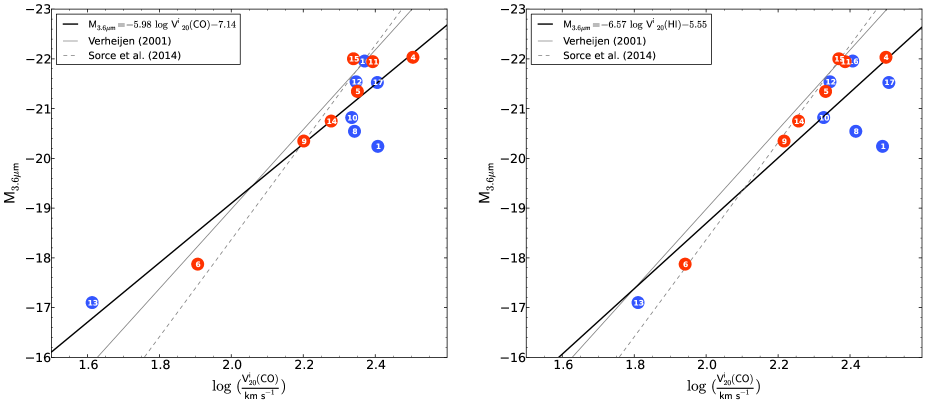
Figure 7.— A comparison of the CO (left-subplot) and H i (right-subplot) TFR for the HERACLES/THINGS sample. The red filled circles denote galaxies whose rotation curves are analysed in this work; the blue filled circles denote the other galaxies in the THINGS/HERACLES sample. The number on each point corresponds to galaxies as numbered in Figure 2. In both subplots we plot the H i TFRs from Verheijen (2001) and Sorce et al. (2014) as a thin grey solid and a dashed line, respectively, for comparison. The best fitting lines from the CO and H i data are plotted in black (thick solid), and the best fit parameters are indicated in the individual subplot legend.

7. Mass Modeling

Mass models of galaxies are used to quantify the contribution of the different constituents to the dynamics, thereby allowing us to model how much dark matter may be present. Mass models are simply the decomposition of the observed rotation curve into the predicted contributions of the visible components combined with a particular dark matter potential.

Consequently, components in mass models traditionally comprise four ingredients - the observed rotation curve, the predicted rotation curves from the stellar and neutral gas components, and a dark matter component usually described by a corresponding halo parameterization. The dark matter halo parameters are adjusted as free parameters to reach the best fit, usually under specific assumptions of the masses of the stellar component (through the stellar mass-to-light ratio, hereafter denoted as $\Upsilon_{*}$) and the gas disk.

Sometimes it is possible to solve for all these parameters simultaneously, i.e., the halo and the disk parameters. In practice this means including $\Upsilon_{*}$ as a free parameter in the fit. However, the uncertainties are large and generally values of $\Upsilon_{*}$ are fixed to reduce the degeneracies in the fit. Since our goal in this section is to quantify the relative impact of the inclusion of molecular gas in mass models, so we do not focus on the pros and cons of particular choices for $\Upsilon_{*}$ or halo models. We refer to dB08 for a full description of the $\Upsilon_{*}$ profiles. We fix $\Upsilon_{*}$ for the disk parameters and solve only for the halo parameters corresponding to the dark matter profiles described below.

We use the CO observations as a proxy for the $\mathrm{H_{2}}$ by converting the CO luminosity to a molecular gas mass surface density through the use of the conversion factor $\mathrm{\alpha_{CO}}$. Radial profiles for $\mathrm{\alpha_{CO}}$ based on a dust-to-gas analysis have been calculated in Sandstrom et al. (2013). We therefore consider two different conversion factors - the commonly used conversion factor based on the Milky Way ($\mathrm{\alpha_{MW}}$), and the values presented in Sandstrom et al. (2013) where available, which we denote as $\mathrm{\alpha_{D2G}}$. The values of $\mathrm{\alpha_{D2G}}$ were derived using observations of CO, dust mass surface density and H i. For some the galaxies the average value $\mathrm{\overline{\alpha}_{D2G}}$ is significantly different than the Milky Way value, as discussed in Section 7.3.

We extend the analysis of the dynamics performed in dB08 by including the contribution of the molecular gas into the mass models of the rotation curve sample indicated in Table 1. As was done in dB08, we exclude NGC 3627 since it hosts a bar and shows signs of tidal interactions with the neighbouring galaxies.

7.1. Method

We use the analysis done in dB08 as a template for this work. However, we only use the photometrically determined $\Upsilon_{*}$ from dB08 and we do not solve for it as a free parameter.

The atomic gas surface density is determined from the integrated H i column density map from the THINGS data, as described in dB08. We use the predicted rotation curves calculated in dB08 as inputs to the mass models in this work. This calculation includes a factor of 1.36 to correct for the presence of Helium. We denote these rotation curves as $V_{\mathrm{g,A}}$.

The predicted stellar rotation curve is calculated using the stellar mass surface density. In some cases this is the sum in quadrature of the disk and bulge components. This is converted from the stellar luminosity profile using the corresponding mass-to-light ratio $\Upsilon_{*}$. We provide a brief discussion of this conversion in Section 7.2. The corresponding predicted rotation curve is denoted as $V_{*}$.

The $\mathrm{H_{2}}$ mass surface density is converted from the observed CO luminosity, and we discuss this procedure in Section 7.3. The resulting predicted rotation curve is denoted as $V_{\mathrm{g,M}}$.

The rotation curve due to the dark matter halo is usually parameterised by a halo model. We discuss the details related to the halo parameters in Section 7.5, and we denote the halo rotation curves as $V_{\mathrm{Halo}}$.

We use the mass surface density of the stars and the respective gas components to calculate predicted rotation curves. These predicted rotation curves show the rotational velocity (as a function of radius) that a test particle would experience due to that particular component alone. We subtract the predicted curves from the observed rotation curve, and fit a halo rotation curve to the residual curve, with the halo parameters as free parameters. We can therefore construct a mass-model relating the contribution of each component to the predicted and observed rotation curves by using the following equation:

$$V_{\mathrm{Obs}}^{2}=V_{\mathrm{g,A}}^{2}+V_{\mathrm{g,M}}^{2}+V_{*}^{2}+V_{\mathrm{Halo}}^{2}$$ (6)

where $V_{\mathrm{obs}}$ denotes the observed rotation curve.

In practice, all the terms on the right hand side of Equation 6 produce a total rotation curve, and this total rotation curve is fitted to the observed rotation curve using a least squares algorithm in the GIPSY task ROTMAS. By varying the characteristic parameters of the dark matter halo parameter a best fitting curve is then derived.

7.2. Stellar Mass Distribution

The stellar mass surface densities are derived using the prescription in dB08. We provide a brief summary here. The $3.6\mu\mathrm{m}$-derived luminosity profiles from the Spitzer Infrared Nearby Galaxy Survey (Kennicutt et al. 2003, SINGS) are used to determine the stellar mass surface density using the $3.6\mu\mathrm{m}$ mass-to-light ratio $\Upsilon_{*}^{3.6}$. The $K$-band mass-to-light ratio $\Upsilon_{*}^{K}$ using the method from Oh et al. (2008). $\Upsilon_{*}^{K}$ is determined from the $J-K$ colors from the 2MASS Large Galaxy Atlas (Jarrett et al. 2003) assuming the models from Bell & de Jong (2001). The derived stellar mass surface density profiles depend on the choice of the initial mass function (IMF). In general, $\Upsilon_{*}^{3.6}$ shows slight radial gradients.

Here we only consider the stellar mass surface densities calculated using the Kroupa IMF (Kroupa 2001). We do not derive fits with $\Upsilon_{*}$ as a free parameter, nor do we adjust the fixed values given in dB08. Changes in $\Upsilon_{*}$ tend to have a large impact on the halo parameters, and these would detract from the more subtle changes due to the inclusion of $\mathrm{H_{2}}$ in the mass models. In that sense we are not trying to improve on the dB08 models by deriving an updated “best” model. Our main goal is to quantify how the (quality of the) fit changes for each galaxy when $\mathrm{H_{2}}$ is included.

7.3. Molecular Gas Distribution

In this section we describe the calculation of the molecular gas mass surface density from the CO observations, using two different conversion factors - the constant Milky Way value and the radially varying values presented in Sandstrom et al. (2013).

The observed CO luminosity $I_{\mathrm{CO}}\,(\mathrm{K\,\,\mathrm{km\,s^{-1}}})$ is converted to $\mathrm{H_{2}}\,(M\mathrm{{}_{\odot}\,pc^{-2}})$ mass surface density using the following relation:

$$\Sigma_{\mathrm{H_{2}}}=\alpha_{\mathrm{CO}}I_{\mathrm{CO}}$$ (7)

This is analogous to the more familiar expression $N_{\mathrm{H_{2}}}(\mathrm{cm^{-2}})=X_{\mathrm{CO}}I_{\mathrm{CO}}$ used to convert CO luminosity to molecular gas column density. The typical value for $X_{\mathrm{CO}}$ for the CO $J=1\rightarrow 0$ transition in the Milky Way is $2\times 10^{20}\,\mathrm{cm^{-2}\,(K\,\,\mathrm{km\,s^{-1}})^{-1}}$ (Dame et al. 2001). The corresponding value for $\alpha_{\mathrm{CO}}$, for the CO $J=2\rightarrow 1$ transition is $6.3\,M\mathrm{{}_{\odot}\,pc^{-2}}\,(\mathrm{K}\,\,\mathrm{km\,s^{-1}})^{-1}$, which we denote as $\mathrm{\alpha_{MW}}$. This assumes a constant CO $J=2\rightarrow 1$ to $J=1\rightarrow 0$ conversion ratio of $0.7$ (Leroy et al. 2013; Sandstrom et al. 2013). The $\alpha_{\mathrm{CO}}$ value quoted here corresponds to the CO $J=2\rightarrow 1$ transition.

Sandstrom et al. (2013) used the HERACLES, THINGS and KINGFISH (Kennicutt et al. 2011, Key Insights into Nearby Galaxies: A Far-Infrared Survey with Herschel) surveys to simultaneously solve for $\alpha_{\mathrm{CO}}$ and the dust-to-gas (D2G) ratio in nearby galaxies, including many that are in our sample. All derived values of $\alpha_{\mathrm{CO}}$ contain a correction of $1.36$ in order to account for the presence of Helium. This correction is also present in the computation of the atomic mass surface density.

We denote the Sandstrom et al. (2013) radially varying conversion factors as $\mathrm{\alpha_{D2G}}$; the corresponding mean value will be denoted as $\mathrm{\overline{\alpha}_{D2G}}$. The values for $\mathrm{\alpha_{CO}}$ vary substantially in the sample and can be very different from the Milky Way value $\mathrm{\alpha_{MW}}=6.3\,M\mathrm{{{}_{\odot}}\,pc^{-2}\,(K\,km\,s^{-1})^{-1}}$. The average values vary from $\mathrm{\overline{\alpha}_{D2G}}=1.4\,M\mathrm{{{}_{\odot}}\,pc^{-2}\,(K\,km\,s^{-1})^{-1}}$ to $\mathrm{\overline{\alpha}_{D2G}}=15.7\,M\mathrm{{{}_{\odot}}\,pc^{-2}\,(K\,km\,s^{-1})^{-1}}$. In addition, the radial profiles of $\mathrm{\alpha_{D2G}}$ presented in Sandstrom et al. (2013) are not flat but usually show a gradual radial increase in the $\mathrm{\alpha_{D2G}}$ value.

In Figure 8 we plot the radial profiles for $\mathrm{\alpha_{D2G}}$ used in this work, based on the data presented in Sandstrom et al. (2013). These radial profiles will be used to calculate the molecular gas mass surface density. In Table 6 we list the average weighted mean $\mathrm{\overline{\alpha}_{D2G}}$ values for the galaxies in our sample.

Binned radial profiles for NGC 2976, NGC 4736, NGC 5055 and NGC 6946 were presented in Sandstrom et al. (2013). For NGC 0925, NGC 2841, NGC 3198, NGC 6946, NGC 7331 we derive radial profiles for $\mathrm{\alpha_{D2G}}$ by binning the individual measurements presented in Sandstrom et al. (2013) in increments of $0.1\,R_{25}$ where $R_{25}$ is the $B$-band isophotal radius at $25\,\mathrm{mag\,arcsec^{-2}}$ presented in that work.

We calculate molecular gas mass surface densities using both the radially dependent $\mathrm{\alpha_{D2G}}$ and the constant Milky Way value for the galaxies in our sample. For NGC 2403 and NGC 2903 we only consider the constant Milky Way value, since these galaxies were not studied in Sandstrom et al. (2013). There is a comparatively higher uncertainty in the $\mathrm{\alpha_{D2G}}$ value for galaxies at higher inclinations, which could be due to opacity effects and the ambiguity in associating specific dust and gas features along the line of sight.

To calculate the molecular gas mass surface density, we use the HERACLES integrated intensity map to calculate the radial surface brightness distribution. For this we use the THINGS tilted-ring geometry from dB08, and we apply an inclination correction. This is used as the input in Equation 7 when calculating the molecular gas mass surface density.

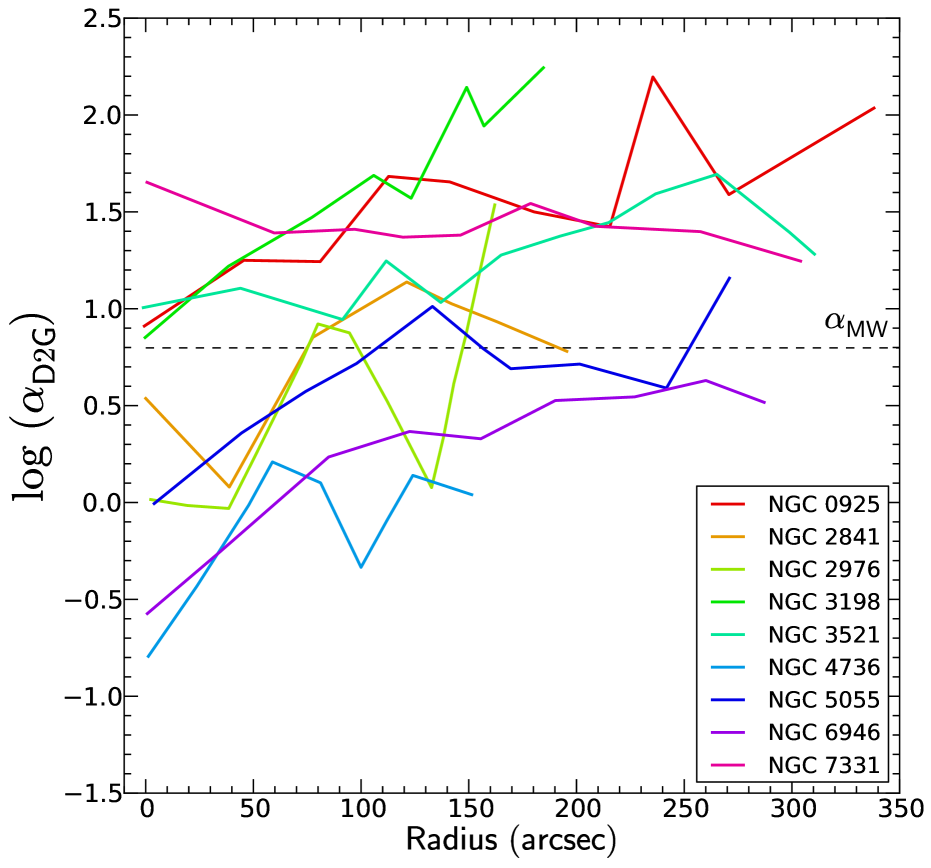
Figure 8.— Radial profiles for $\log\,(\mathrm{\alpha_{D2G}})$ used to convert $I_{\mathrm{CO}}$ to $\Sigma_{\mathrm{H_{2}}}$ for galaxies in this work. The CO $J=2\rightarrow 1$ values for $\mathrm{\alpha_{D2G}}$ are plotted here. The Milky Way value of $\mathrm{\alpha_{MW}}=6.3\,M\mathrm{{{}_{\odot}}\,pc^{-2}\,(K\,km\,s^{-1})^{-1}}$ is indicated as a dashed horizontal line. For NGC 2976, NGC 4736, NGC 5055 and NGC 6946 we use the profiles corresponding to those presented in Figure 7 of Sandstrom et al. (2013). For NGC 0925, NGC 2841, NGC 3198, NGC 3521 and NGC 5055 we derive profiles by binning the individual data points in Figure 22 in Sandstrom et al. (2013) in increments of $R_{25}$, where $R_{25}$ is the $B$-band isophotal radius at $25\,\mathrm{mag\,arcsec^{-2}}$ presented in that paper.

Table 6The average value of the CO-to-$\mathrm{H_{2}}$ conversion factors $\mathrm{\overline{\alpha}_{D2G}}$.

Galaxy	$\mathrm{\mathrm{\overline{\alpha}_{D2G}}}$
	$M\mathrm{{{}_{\odot}}\,pc^{-2}\,(K\,km\,s^{-1})^{-1}}$
NGC 0925	14.3
NGC 2841	7.1
NGC 2976	4.7
NGC 3198	15.7
NGC 3521	10.9
NGC 4736	1.4
NGC 5055	5.3
NGC 6946	2.9
NGC 7331	14.0

7.4. Putting it all together

The mass surface densities computed using the methods described above are then used to calculate the predicted rotation curves (i.e., $V_{\mathrm{g,A}}$, $V_{\mathrm{g,M}}$ and $V_{*}$) by using the GIPSY task ROTMOD. de Blok et al. (2008) assume an infinitely thin disk for the H i and a $\mathrm{sech^{2}}$ distribution for the stellar component, and we do the same here. The stellar predicted rotation curves were derived using mass surface densities calculated from photometrically determined $\Upsilon_{*}$. We assume that the CO is also distributed in an infinitely thin disk. The predicted rotation curves are inserted into the mass-model in Equation 6. The parameterised halo rotation curve is then fitted to the observed rotation curve. Therefore, the only free parameters in our fits are the dark-matter halo parameters, discussed below.

7.5. Dark Matter mass models

We compute mass-models using both the Navarro-Frenk-White (NFW) halo (Navarro et al. 1996, 1997) and the observationally motivated pseudo-isothermal (ISO) halo.

Following Navarro et al. (1996, 1997) the NFW mass-density distribution has the form

$$\rho_{\mathrm{NFW}}(R)=\frac{\rho_{\mathrm{i}}}{(R/R_{\mathrm{s}})(1+R/R_{\mathrm{s}})^{2}}$$ (8)

where $R_{\mathrm{s}}$ is the scale radius of the halo (and $\rho_{\mathrm{i}}$ is proportional to the density of the universe at the time of collapse of the dark matter halo. This leads to a halo rotation curve (Navarro et al. 1996) given by:

$$V(R)=V_{200}\left[\frac{\ln(1+cx)-cx/(1+cx)}{x[\ln(1+c)-c/(1+c)]}\right]^{1/2}$$ (9)

where $x=R/R_{200}$, $c=R_{200}/R_{\mathrm{s}}$ is the concentration parameter and $V_{200}$ is the characteristic velocity at radius $R_{200}$, the radius where the density contrast relative to the critical density of the universe exceeds $200$. Cosmologically motivated values for the halo parameters can be deduced using the simulations from Bullock et al. (2001) and the models from Spergel et al. (2007). We solve for $c$ and $V_{200}$ by fitting $V(R)$ to Equation 6.

The ISO mass-density distribution has the form

$$\rho_{ISO}(R)=\rho_{0}\left[1+\left(\frac{R}{R_{c}}\right)^{2}\right]^{-1}$$ (10)

where $\rho_{0}$ denotes the central density of the halo and $R_{\mathrm{c}}$ is the so-called core radius. This leads to a halo rotation curve given by:

$$V(R)=\left[4\pi G\rho_{0}R_{c}^{2}\left(1-\frac{R_{c}}{R}\arctan\left(\frac{R}{R_{c}}\right)\right)\right]^{1/2}$$ (11)

where the asymptotic velocity of the halo, $V_{\infty}$ is given by:

$$V_{\infty}=\sqrt{4\pi G\rho_{0}R_{c}^{2}}$$ (12)

For the ISO case we can directly solve for $\rho_{0}$ and $R_{\mathrm{c}}$ by fitting $V(R)$ to the parent Equation 6.

We use the GIPSY task ROTMAS to fit the respective halo rotation curves to the mass model in 6. We use the observed rotation curve error-bars to weight the fits. This is done to keep our results consistent with dB08. Adopting a different weighting scheme, such as uniform errorbars for all points has little impact on the outcomes of this study.

8. Results - Mass Models

In this section we present the mass models for each galaxy in our sample, assuming either an NFW or ISO halo form. The corresponding halo parameters are presented in Tables 7 and 8.

For a few galaxies the HERACLES rotation curve is either steeper in the inner parts than the THINGS curve (e.g., NGC 5055) or fills in the inner part of the rotation curve where no H i has been detected (e.g., NGC 4736 — see Appendix for full description). In these cases we also explore fits to a hybrid rotation curve, where we use the HERACLES rotation curve in the inner few kpc and the THINGS rotation curve at larger radii. In the text we refer to the hybrid rotation curves as the HERACLES/THINGS or COH i rotation curves. We refer to the observed H i rotation curves as the THINGS rotation curves, and to the observed CO rotation curves as the HERACLES rotation curves.

In each case we compare our results with those from dB08. It is important to note that dB08 considered mass models comprising stellar rotation curves predicted using both “diet” Salpeter (Salpeter 1955; Bell & de Jong 2001) and Kroupa IMFs. For a given mass-to-light ratio $\mathrm{M/L_{*}}$ the difference between the Kroupa and diet Salpeter is $\sim 0.15$ dex. While dB08 list derived halo parameters for both these IMFs, their figures only show the diet Salpeter mass models. Here we only consider Kroupa IMF based models, so this difference should be kept in mind when comparing the mass models presented in this work with those in dB08.

When dealing with the rotation curves $V_{\mathrm{g,A}}$ and $V_{\mathrm{g,M}}$, we adopt the convention of plotting negative values of $V^{2}$ as negative values of $V$. Such values can occur since, in the presence of central under-densities, test particles in or near such an under-density will experience an outward force.

8.1. NGC 925

In Figure 9 we plot the best fitting models using the THINGS rotation curve. The stellar mass distribution comprises only a single component, and is the dominant component within $5\mathrm{\,kpc}$. At greater radii the dark matter distribution becomes more important.

The value $\mathrm{\overline{\alpha}_{D2G}}=14.3\,M\mathrm{{{}_{\odot}}\,pc^{-2}\,(K\,km\,s^{-1})^{-1}}$ is much larger than the Milky Way value. The predicted molecular gas rotation curves using $\mathrm{\alpha_{MW}}$ and $\mathrm{\alpha_{D2G}}$ do not exceed a maximum of $\sim 10\,\mathrm{km\,s^{-1}}$ at $\sim 3\mathrm{\,kpc}$. The $\mathrm{\alpha_{D2G}}$ curve is slightly higher than the $\mathrm{\alpha_{MW}}$ curve, but not sufficiently to change the predicted molecular gas rotation curve due to the small amount of molecular gas detected. Although fitting the NFW rotation curve produces a halo model which appears reasonable, the fit yields unrealistic halo parameters: $c<1$ and correspondingly high values for $V_{200}>200\,\mathrm{km\,s^{-1}}$, which is substantially different from the expected range (Bullock et al. 2001). The NFW fit is therefore shown for illustrative purposes and will not be considered in further analysis.

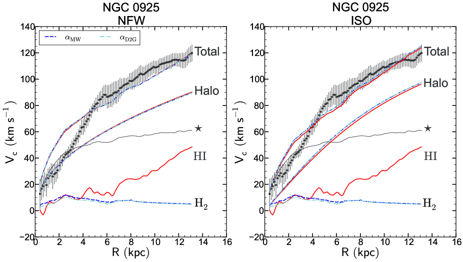
Figure 9.— NGC 0925 mass models using the THINGS rotation curve. Results using the NFW model are in the left panel, results using the ISO model are in the right panel. The observed rotation curve is plotted as grey filled circles with errorbars. The predicted stellar rotation curve $V_{*}$ is plotted as a thin grey line, and is labelled by the $\star$ in the figure. The predicted atomic gas rotation curve $V_{\mathrm{g,A}}$ is plotted as a thicker red line, and is labelled as $\mathrm{HI}$ in the figure. The predicted molecular gas rotation curves $V_{\mathrm{g,M}}$ are plotted as dashed-dotted cyan ($\alpha_{D2G}$) and dashed blue lines ($\alpha_{MW}$), and are labelled as $\mathrm{H_{2}}$ in the figure. The dark matter halo rotation curves $V_{\mathrm{Halo}}$ and the resultant rotation curves fits to $V_{\mathrm{Obs}}$ for either choice of $\mathrm{\alpha_{CO}}$ are plotted using this convention, labelled as Halo and Total in the figure, respectively. The $V_{\mathrm{Halo}}$ rotation curve and the consequent fit to $V_{\mathrm{Obs}}$ from dB08 (i.e., no molecular gas) are both plotted as red solid lines.

8.2. NGC 2403

In Figures 10 and 11 we plot the results of the mass modelling for NGC 2403. NFW and ISO halo models were fitted to the THINGS H i observed rotation curve.

The stellar mass distribution can be described by either a 1- or 2-component decomposition. We fit halo rotation curves using both stellar distributions, treating the 1- and 2-component models separately.

Sandstrom et al. (2013) did not solve for a $\mathrm{\alpha_{D2G}}$ value for NGC 2403. We therefore only consider a predicted molecular gas rotation curve using $\mathrm{\alpha_{MW}}$. This rotation curve reaches a maximum of $\sim 10\,\mathrm{km\,s^{-1}}$ at $\sim 4\mathrm{\,kpc}$ and declines thereafter. The molecular gas predicted rotation curve is only slightly higher than the H i rotation curve within $\sim 3\mathrm{\,kpc}$, but is overall the smallest contributor to the dynamics of NGC 2403.

For fits using the NFW model the addition of the molecular gas makes no difference to the model and total rotation curves. The NFW total rotation curve is slightly lower than the observed rotation curve at $1\mathrm{\,kpc}$, but shows an overall good fit to the observed rotation curve. For fits using the ISO model the addition of the molecular gas makes no difference to the best fitting model and consequent total rotation curves. The ISO models do not fit the inner part (within $2\mathrm{\,kpc}$) of the observed rotation curve as well as the NFW models. The quality of the fits for both the NFW and ISO fits including molecular gas are no different from the H i-only case.

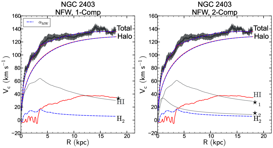
Figure 10.— NGC 2403 mass models using the HERACLES/THINGS data with an NFW halo. Results using 1- and 2-component stellar distributions are plotted in the left and right panels respectively. Line styles and colours are as in Figure 9.

Figure 11.— NGC 2403 mass models using the HERACLES/THINGS data with an ISO halo. Results using 1- and 2-component stellar distributions are plotted in the left and right panels respectively. Line styles and colours are as in Figure 9.

8.3. NGC 2841

In Figure 12 we plot the results of the mass modelling for NGC 2841. ISO and NFW halo models were fitted using the THINGS H i observed rotation curve.

We fit models to the THINGS rotation curve, which starts at $\sim 4\mathrm{\,kpc}$ and extends to $\sim 50\mathrm{\,kpc}$. The stellar mass distribution is decomposed into 2-components, which we use to fit the observed rotation curve.

The value $\mathrm{\overline{\alpha}_{D2G}}=7.1\,M\mathrm{{{}_{\odot}}\,pc^{-2}\,(K\,km\,s^{-1})^{-1}}$ is very close the Milky Way value. The predicted rotation curves for both $\mathrm{\alpha_{D2G}}$ and $\mathrm{\alpha_{MW}}$ are almost identical, as are the resultant best fitting halo model rotation curves for both the NFW and ISO cases. The molecular gas mass surface density produces a maximum velocity of $\sim 20\,\mathrm{km\,s^{-1}}$. Although the predicted molecular gas rotation velocities are small in comparison to the other components, the resultant halo model rotation curves which include molecular gas are different from the H i-only rotation curves. The effect of adding molecular gas is to increase the amplitude of the halo rotation curves. The total rotation curve with added molecular gas is almost identical to the H i-only total rotation curve, showing small differences at the innermost radii.

As anticipated, the $c$, $V_{200}$ and $\mathrm{\chi^{2}_{r}}$ values for $\mathrm{\alpha_{D2G}}$ and $\mathrm{\alpha_{MW}}$ predicted rotation curves are nearly identical. The values of $c$ are higher than the H i-only case, while the $V_{200}$ values are slightly smaller.

The addition of $\mathrm{H_{2}}$ slightly increases the $\mathrm{\chi^{2}_{r}}$ values when fitting the ISO models.

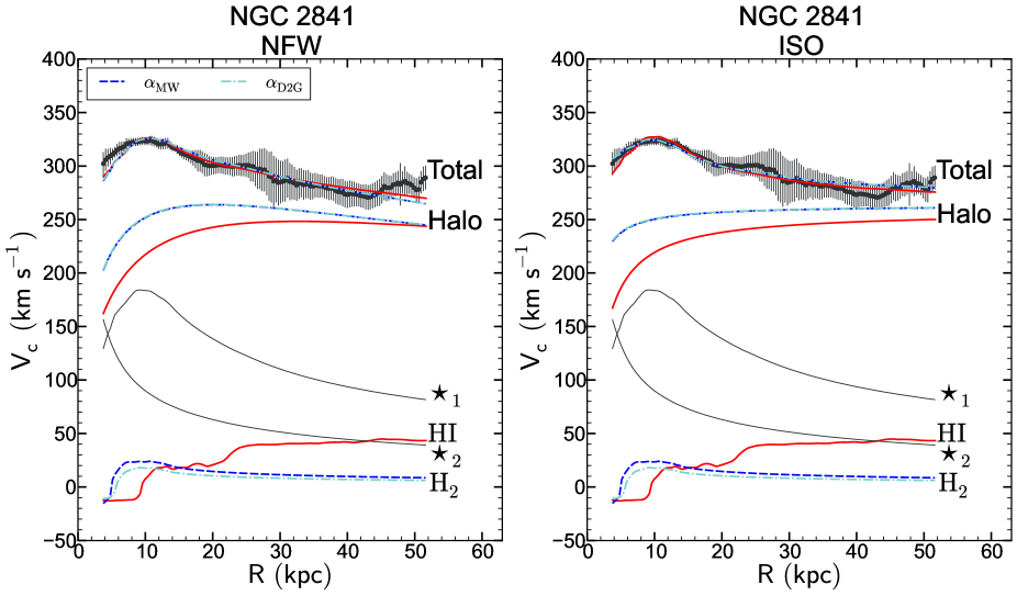
Figure 12.— NGC 2841 mass models using the HERACLES/THINGS data. Results with the NFW halo are in the left panel, results with the ISO halo are in the right panel. Line styles and colours are as in Figure 9.

8.4. NGC 2903

The results of the mass modelling for NGC 2903 are plotted in Figure 13. An NFW halo model was fitted to the outer regions using the THINGS H i observed rotation curve, as described in the Appendix.

NGC 2903 hosts a strong bar and the rotation curve in the inner $3\mathrm{\,kpc}$ for the H i and CO are strongly affected by streaming motions. The stellar mass surface density is described using a 2-component decomposition.

We do not use the rotation curve corrected for the bar-streaming motions derived in Section 5.1. In order to do this we would need to do an associated correction of the surface brightness distribution, which is beyond the scope of this work. We therefore adopt the same strategy as in dB08, fitting mass models to the observed rotation curves for radii larger than $3\mathrm{\,kpc}$.

We plot the results of fitting the NFW halo. Attempting to fit the ISO halo model rotation curve converges to unrealistic values for the halo parameters - $R_{\mathrm{c}}\ll 1$ and a correspondingly large value for $\rho_{0}\gg 1000$. This is because there are no constraints from the inner parts of the rotation curve.

Sandstrom et al. (2013) did not solve for a $\mathrm{\alpha_{D2G}}$ value for NGC 2903. We therefore only consider a predicted molecular gas rotation curve using $\mathrm{\alpha_{MW}}$. The predicted molecular gas rotation curve reaches a maximum of $\sim 40\,\mathrm{km\,s^{-1}}$ at a radius $\sim 5\mathrm{\,kpc}$, and declines to approximately $10\,\mathrm{km\,s^{-1}}$ at larger radii.

The velocities of the halo rotation curve are slightly higher than for those of H i-only case. The total rotation curve is identical to the H i-only total rotation curve. The values for $c$ and $V_{200}$ are almost identical in both cases, as are the $\mathrm{\chi^{2}_{r}}$ values. The total rotation curves produce good fits to the observed THINGS rotation curve.

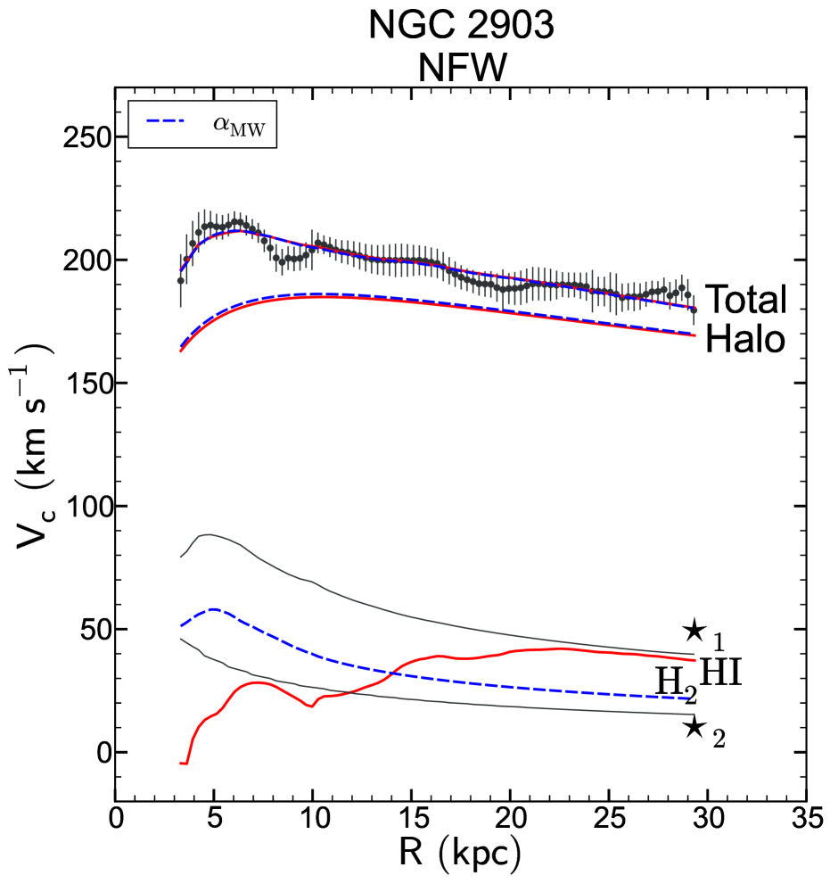
Figure 13.— NGC 2903 mass models using the HERACLES/THINGS data with the NFW halo. Line styles and colours are as in Figure 9.

8.5. NGC 2976

In Figure 14 we plot the results of the mass modelling for NGC 2976. The ISO halo model was fitted using the THINGS H i rotation curve. Fitting the NFW halo model converge to unrealistic values of halo parameters. This was also the case for the H i-only fits in dB08.

The stellar mass surface density comprises a single component, and we use this to fit our rotation curves.

While the average value of $\mathrm{\overline{\alpha}_{D2G}}=4.7\,M\mathrm{{{}_{\odot}}\,pc^{-2}\,(K\,km\,s^{-1})^{-1}}$ value is very similar to the $\mathrm{\alpha_{MW}}$, the radial profile of $\mathrm{\alpha_{D2G}}$ is steep in the inner part and leads to a much lower molecular gas mass surface density. As such, the predicted molecular gas rotation curve with $\mathrm{\alpha_{D2G}}$ is very different in comparison to that calculated with $\mathrm{\alpha_{MW}}$. The molecular gas contribution to the dynamics is very small and the stellar component makes the largest contribution to the model. Therefore, the addition of the molecular gas does not make an appreciable difference to the halo rotation curves and the fitted total rotation curves.

The fitted ISO parameters are similar to the H i-only case for either choice of $\mathrm{\alpha_{CO}}$, suggesting that the molecular gas makes a negligible contribution to the dynamics of NGC 2976.

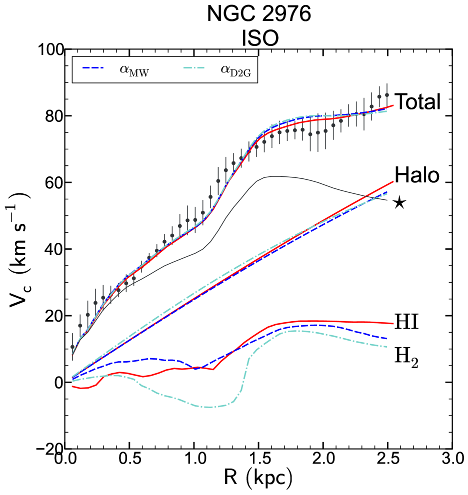
Figure 14.— from NGC 2976 mass models using the THINGS data with the ISO halo. Line styles and colours for each plot are as in Figure 9.

8.6. NGC 3198

In Figures 15 and 16 we plot the results of the mass modelling for NGC 3198. For NGC 3198 we use 1- and 2-component decompositions of the stellar surface brightness distribution to derive the predicted stellar rotation curves, and we treat the 1- and 2-component cases separately.

In the analysis of the observed rotation curves for NGC 3198 presented in the Appendix we note a considerable difference in the shapes between the H i and CO observed rotation curves within $4\mathrm{\,kpc}$. We therefore consider two observed rotation curves for NGC 3198 - the THINGS rotation curve and a hybrid HERACLES/THINGS rotation curve, where we use the HERACLES rotation curve inside $4\mathrm{\,kpc}$ and the THINGS rotation curve outside this radius. Therefore, for both the NFW and ISO models we have four scenarios, corresponding to the two possible stellar decompositions and the two observed rotation curves.

For NGC 3198 the conversion factor $\mathrm{\overline{\alpha}_{D2G}}=15.7\,M\mathrm{{{}_{\odot}}\,pc^{-2}\,(K\,km\,s^{-1})^{-1}}$ is considerably higher than the Milky Way value. The predicted molecular gas rotation curves are identical within $\sim 5\mathrm{\,kpc}$, but the $\mathrm{\alpha_{D2G}}$ molecular gas rotation curve is much higher than the $\mathrm{\alpha_{MW}}$ rotation curve between $5\sim 10\mathrm{\,kpc}$. For the NFW case the halo rotation curves with added molecular gas are identical to the H i-only case. The NFW halo parameters presented in Table 7 are similar for models with and without molecular gas (within the uncertainties).

Fitting the ISO halo to the 1-component stellar distribution results in halo rotation curves which have a slightly different shape than the H i-only case, and which are steeper than the H i-only halo rotation curve within $5\mathrm{\,kpc}$, and flatter at larger radii. The $\mathrm{\alpha_{MW}}$ and $\mathrm{\alpha_{D2G}}$ predicted molecular gas rotation are identical. For the fits to the ISO halo with the 2-component stellar distribution the halo rotation curves with added molecular gas are identical to the H i-only halo rotation curve.

In general, better fits were achieved for the 1-component stellar distribution as compared to the 2-component distribution. Fitting the ISO halo produces better fits compared to the NFW halo.

For all ISO fits the $R_{C}$ and $\rho_{0}$ values are fairly similar, while the 1- and 2-component fits with H i-only show completely different parameters. For the NFW fits the values for $c$ and $V_{200}$ are tightly constrained and do not vary much for either of 1- or 2-component stellar models. The quality of the fits are similar to the H i-only case.

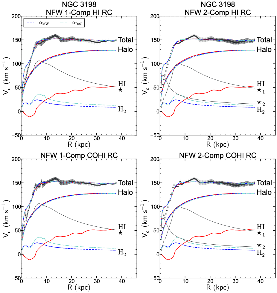
Figure 15.— NGC 3198 mass models with the NFW halo. Fits using 1- and 2-component stellar distributions are plotted in the left and right panels respectively, for each row. Fits to the THINGS rotation curve are plotted in the top row, fits to the HERACLES/THINGS rotation curve are plotted in the bottom row. Line styles and colours for each plot are as in Figure 9.

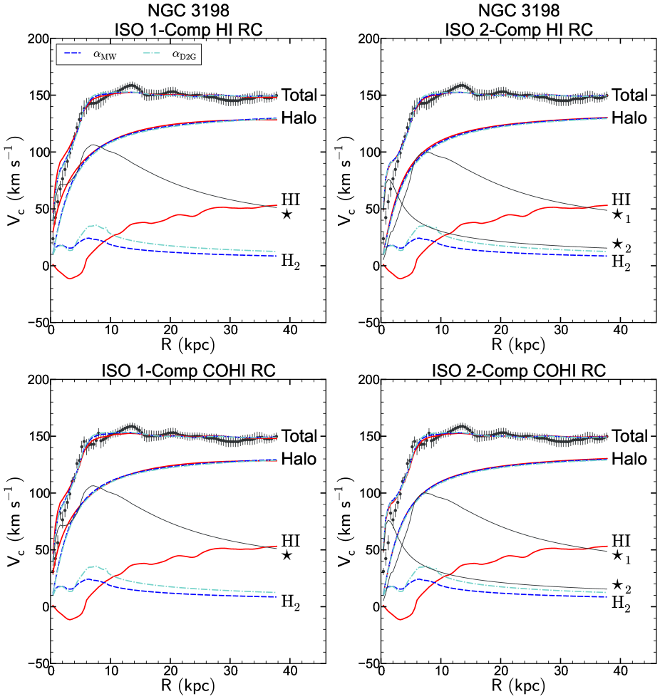
Figure 16.— NGC 3198 mass models using the ISO halo. Fits using 1- and 2-component stellar distributions are plotted in the left and right panels respectively, for each row. Fits to the THINGS rotation curve are plotted in the top row, fits to the HERACLES/THINGS rotation curve are plotted in the bottom row. Line styles and colours for each plot are as in Figure 9.

8.7. NGC 3521

In Figures 17 and 18 we plot the predicted, model and best fitting rotation curves for NGC 3521. For NGC 3521 we use a single component stellar decomposition.

The HERACLES rotation curve is steeper within $4\mathrm{\,kpc}$. We therefore consider two observed rotation curves when fitting ISO and NFW models - a THINGS rotation curve and a HERACLES/THINGS rotation where we use the HERACLES rotation curve within $4\mathrm{\,kpc}$ and the THINGS rotation curves for larger radii.

NGC 3521 contains a considerable amount of molecular gas in comparison to the other galaxies in this sample. In Leroy et al. (2008) the mass surface densities are plotted, showing that the molecular gas surface density reaches $\sim 50\,M\mathrm{{}_{\odot}\,pc^{-2}}$. The resultant predicted molecular gas rotation curve using $\mathrm{\alpha_{D2G}}$ rises steeply within $5\mathrm{\,kpc}$ and reaches a maximum of $\sim 70\,\mathrm{km\,s^{-1}}$.

For both the NFW and ISO fits, the addition of molecular gas leads to better fits as compared to the H i-only case (cf. Tables 7 and 8). In Figures 17 and 18, we see that fitting halo models to the HERACLES/THINGS rotation curves yield better results than when using the THINGS rotation curve.

We obtain the best fits when fitting to the ISO halo. The fits using either $\mathrm{\alpha_{D2G}}$ and the Milky Way value are similar in this case, and produce halo rotation curves which are considerably different from the H i-only case.

Figure 17.— NGC 3521 mass models with an NFW halo. Fits to the THINGS rotation curve are plotted in the left panel, fits to the HERACLES/THINGS rotation curve are plotted in the right panel. Line styles and colours for each plot are as in Figure 9.

Figure 18.— NGC 3521 mass models with an ISO halo. Fits to the THINGS rotation curve are plotted in the left panel, fits to the HERACLES/THINGS rotation curve are plotted in the right panel. Line styles and colours for each plot are as in Figure 9.

8.8. NGC 4736

In Figure 19 we plot the results from the mass modelling for NGC 4736.

Fits using the ISO halos did not converge and resulted in unrealistic fits with $R_{c}\ll 1$ and $\rho_{0}\gg 1000$, which is most likely due to a sharp decline in the outer part of the rotation curve. We therefore only include results for the NFW halo. For NGC 4736 we use a 2-component stellar decomposition to calculate the stellar predicted rotation curves.

There is a deficiency of H i in the centre of NGC 4736. Correspondingly, the molecular gas distribution peaks in the centre of NGC 4736, with the maximum molecular gas mass surface density reaching $\sim 100\,M\mathrm{{}_{\odot}\,pc^{-2}}$ (Leroy et al. 2008) using the Milky Way conversion factor. We therefore consider two observed rotation curves in this work - the THINGS rotation curve which extends from $\sim 0.5\mathrm{\,kpc}$ outwards and does not track the inner slope of the rotation curve, and a hybrid HERACLES/THINGS rotation curve where we use the HERACLES rotation curve within $\sim 1\mathrm{\,kpc}$ and the THINGS rotation curve outside this radius. The average value $\mathrm{\overline{\alpha}_{D2G}}=1.4\,M\mathrm{{{}_{\odot}}\,pc^{-2}\,(K\,km\,s^{-1})^{-1}}$ is significantly smaller than the Milky Way value. This is reflected in Figure 19 - the predicted molecular gas rotation curve using the Milky Way conversion factor reaches a maximum of $\sim 40\,\mathrm{km\,s^{-1}}$ while the predicted rotation curve using $\mathrm{\alpha_{D2G}}$ does not exceed $\sim 20\,\mathrm{km\,s^{-1}}$.

The predicted molecular gas rotation curves are significantly different for the assumed values of $\mathrm{\alpha_{CO}}$. In addition, mass models using the THINGS rotation curve are significantly better than those using the HERACLES/THINGS rotation curve.

There are several factors which make interpretation of the results for this galaxy difficult, as already identified in dB08. Firstly, there is a large uncertainty in the $\Upsilon_{*}$ values for the central bulge-like component. Secondly, Trachternach et al. (2008) find evidence for large non-circular motions in this galaxy, which are also evident as the large spread in velocities along the minor-axis pV diagram in Figure 34.

Another important factor is the declining rotation curve, which presents difficulties when fitting either the ISO or the NFW haloes, neither of which were “designed” to do so. Fitting the ISO halo leads to an extremely compact core, and fitting the NFW halo implies a highly concentrated profile.

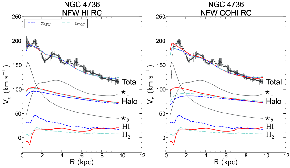
Figure 19.— NGC 4736 mass models with an NFW halo. Fits to the THINGS rotation curve are plotted in the left panel, fits to the HERACLES/THINGS rotation curve are plotted in the right pane. Line styles and colours for each plot are as in Figure 9.

8.9. NGC 5055

In Figure 20 we plot the results of the mass modelling for NGC 5055. For NGC 5055 we use a 2-component stellar decomposition to determine the predicted stellar rotation curves.

For NGC 5055 $\mathrm{\overline{\alpha}_{D2G}}=5.3\,M\mathrm{{{}_{\odot}}\,pc^{-2}\,(K\,km\,s^{-1})^{-1}}$, which is very close to the Milky Way value. However, the radial profiles for $\mathrm{\alpha_{D2G}}$ shows a depression in the central region, which leads to a substantially different $\mathrm{\alpha_{D2G}}$ rotation curve in the inner $5\mathrm{\,kpc}$, as compared to using a single $\mathrm{\alpha_{MW}}$ value for the conversion.

The HERACLES rotation curve is steeper in the inner $5\mathrm{\,kpc}$. We therefore consider two observed rotation curves in our fits — the THINGS rotation curve and a HERACLES/THINGS rotation curve assembled by using the HERACLES rotation curve within $5\mathrm{\,kpc}$ and switching over to the THINGS rotation curve for larger radii.

Fits to the NFW halo did not converge to reasonable values. We therefore only plot the fits to the ISO halo.

Using the ISO profile produces reasonable values of $\rho_{0}$ and $R_{C}$. Fitting to either the THINGS or HERACLES/THINGS curves yields comparable values of $\mathrm{\chi^{2}_{r}}$. The values for $\rho_{0}$ and $R_{C}$ are different from the H i-only case, which is evident in the different shapes of the halo rotation curves.

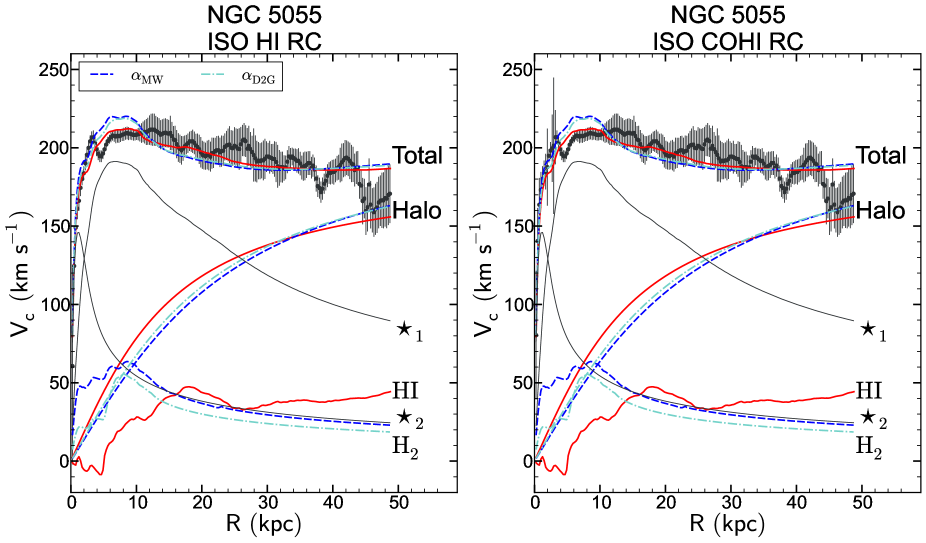
Figure 20.— NGC 5055 mass models with an ISO halo. Fits to the THINGS rotation curve are plotted in the left panel, fits to the HERACLES/THINGS rotation curve are plotted in the right pane. Line styles and colours for each plot are as in Figure 9.

8.10. NGC 6946

In Figures 21 and 22 we plot the results of the mass modelling for NGC 6946 for the NFW and ISO halos respectively. For NGC 6946 we use a 2-component stellar decomposition to determine the stellar predicted rotation curves.

NGC 6946 has a large amount of CO detected. Using the Milky Way conversion factor, Leroy et al. (2008) showed that the molecular gas mass surface density is as high as $\sim 400\,M\mathrm{{}_{\odot}\,pc^{-2}}$. This corresponds to a molecular gas predicted rotation curve which reaches a maximum of $\sim 60\,\mathrm{km\,s^{-1}}$ at approximately $1\mathrm{\,kpc}$. The CO emission shows a compact, bulge like distribution (Leroy et al. 2008), similar to the stellar component.

The H i observations show a deficiency in the centre of NGC 6946, where we find an abundance of CO. This allows us to fill in the inner part of the rotation curve using the HERACLES rotation curve. We therefore consider two rotation curves: the THINGS rotation curve, which starts from approximately $1\mathrm{\,kpc}$ and the HERACLES/THINGS rotation curve where we use the HERACLES curve in the inner $1\mathrm{\,kpc}$.

In both the NFW and ISO cases the fitted total rotation curve significantly overshoots the inner part of the HERACLES/THINGS rotation curve. As with NGC 4736, the $\Upsilon_{*}$ value has a large uncertainty.

For fits using the NFW halo the addition of the molecular gas leads to a large difference in the derived parameters. Using the predicted molecular gas rotation curve with $\mathrm{\alpha_{MW}}$ leads to a poor fit, so we do not plot the results here, neither do we include them in Table 7.

For fits using the ISO halo to the THINGS rotation curve the $\mathrm{\chi^{2}_{r}}$ is slightly better upon the addition of $\mathrm{H_{2}}$.

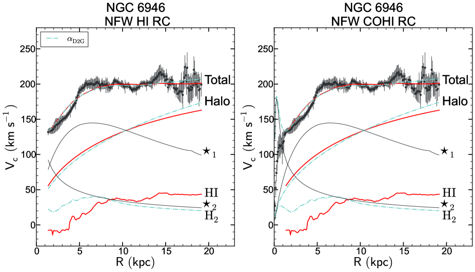
Figure 21.— from NGC 6946 mass models with an NFW halo. Fits to the THINGS rotation curve are plotted in the left panel, fits to the HERACLES/THINGS rotation curve are plotted in the right pane. Line styles and colours for each plot are as in Figure 9.

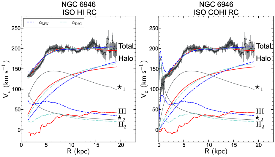
Figure 22.— NGC 6946 mass models with an ISO halo. Fits to the THINGS rotation curve are plotted in the left panel, fits to the HERACLES/THINGS rotation curve are plotted in the right pane. Line styles and colours for each plot are as in Figure 9.

8.11. NGC 7331

In Figure 23 we plot the results of the mass modelling for NGC 7331 using the NFW halo. For NGC 7331 we use a 2-component stellar decomposition to determine the stellar predicted rotation curves.

Our general method has been to use a photometrically determined $\Upsilon_{*}$ with a Kroupa IMF to calculate the stellar mass surface density. However, for NGC 7331 this combination of $\Upsilon_{*}$ and IMF predicts disks which are too massive which leads to predicted stellar rotation curves which are much higher than the observed rotation curve (see dB08).

dB08 addressed this by using a radially constant value of $\Upsilon_{*}$ for each stellar component when determining the stellar mass surface density. This leads to reasonable fits to the observed rotation curve. We use these stellar mass surface densities to calculate the predicted stellar rotation curves.

For NGC 7331 $\mathrm{\overline{\alpha}_{D2G}}=14.0\,M\mathrm{{{}_{\odot}}\,pc^{-2}\,(K\,km\,s^{-1})^{-1}}$ is much larger than the Milky Way value. Leroy et al. (2008) showed that the $\mathrm{H_{2}}$ mass surface density peaks at slightly more than $20\,M\mathrm{{}_{\odot}\,pc^{-2}}$ assuming $\mathrm{\alpha_{MW}}$, and is concentrated on a ring at approximately $3\mathrm{\,kpc}$ away from the centre of the galaxy. The predicted molecular gas rotation curve shows a maximum of $\sim 70\,\mathrm{km\,s^{-1}}$ using $\mathrm{\alpha_{D2G}}$, and a maximum of $\sim 40\,\mathrm{km\,s^{-1}}$ using $\mathrm{\alpha_{MW}}$.

The H i shows a deficiency in the centre, and although the CO shows a similar depression, there is sufficient emission detected for a CO rotation curve to be derived. We therefore consider both an H i-only THINGS rotation curve and a hybrid HERACLES/THINGS rotation curve.

In Figure 23 we show the fit using the NFW model rotation curves using the predicted molecular gas rotation curve derived using $\mathrm{\alpha_{MW}}$. This shows that the H i-only fits overshoot the observed rotation curve within $\sim 20\mathrm{\,kpc}$.

Attempting to fit a mass model using an ISO halo model does not lead to convergence and results in severely unrealistic values of the halo parameters, and are not plotted here.

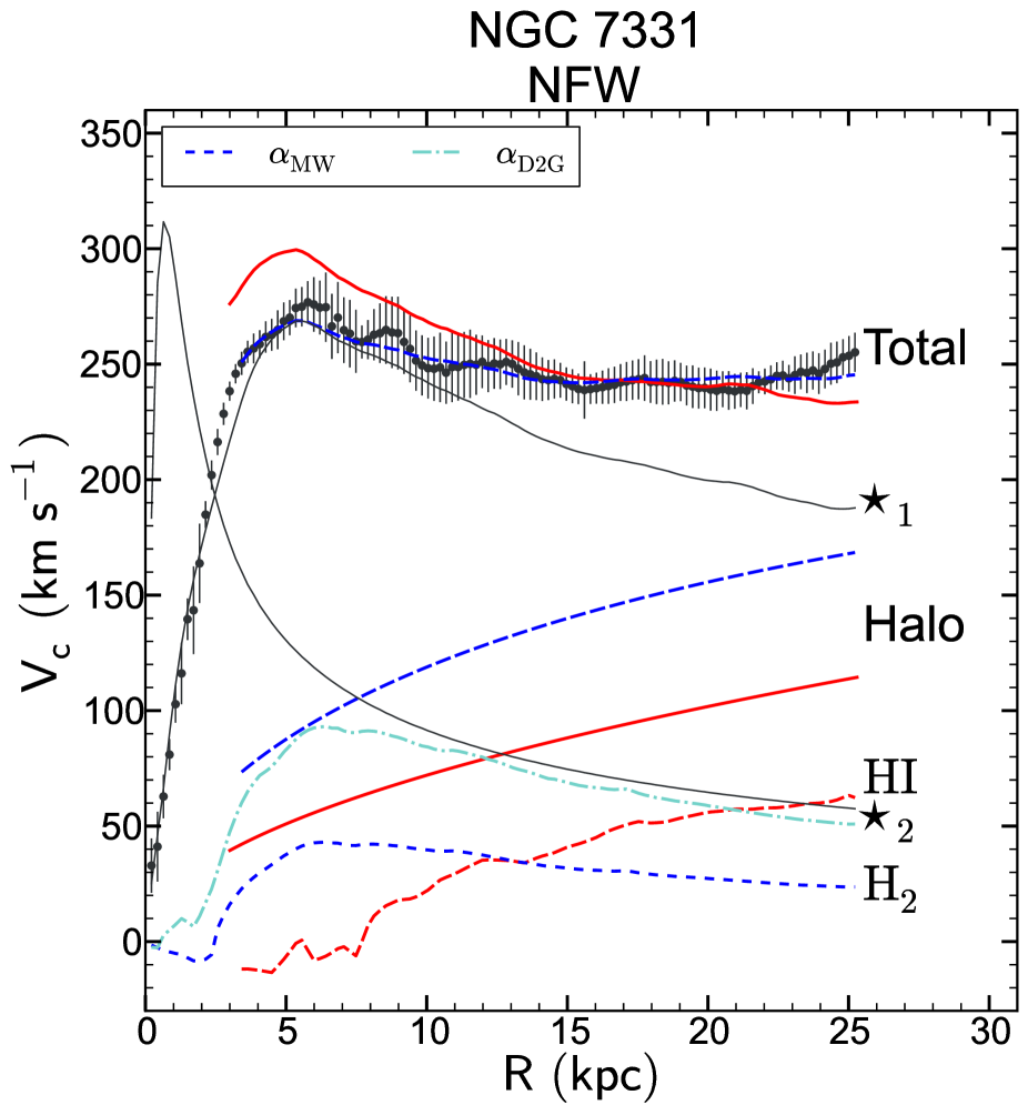
Figure 23.— NGC 7331 mass models with an NFW halo to the hybrid HERACLES/THINGS rotation curve. Line styles and colours are as in Figure 9.

9. Summary

We summarize the mass model parameters for the NFW and ISO fits in Tables 7 and 8 respectively.

We plot the NFW parameters from Table 7 in Figure 24 for both the models with and without molecular gas. We also plot the expected values using $\mathrm{\Lambda CDM}$ parameters (de Blok et al. 2003) and the $1\,\sigma$ and $2\,\sigma$ scatter from Bullock et al. (2001). This plot shows that the NFW halo parameters for NGC 2403, NGC 3198, NGC 3521 and NGC 6946 lie within the $1\,\sigma$ region for the H i-only case. The addition of the molecular gas pushes these values away from the region of expected values.

We plot the ISO parameters from Table 8 in Figure 25 for both the models with and without molecular gas. We plot the expected values suggested by Kormendy & Freeman (2004) and the region corresponding to a $1\,\sigma$ and $2\,\sigma$ scatter. Here there is no systematic trend in the parameters upon the addition of molecular gas.

In Figures 24 and 25 we plot parameters corresponding to the model which produces the lowest $\mathrm{\chi^{2}_{r}}$ for each galaxy, for each value of $\alpha_{\mathrm{CO}}$.

It is important to note the difference in the predicted velocities for the molecular gas rotation curves that arises from a different choice of $\mathrm{\alpha_{CO}}$. For some galaxies the $\mathrm{\alpha_{MW}}$ and $\mathrm{\alpha_{D2G}}$ predicted molecular gas rotation curves are very similar, e.g., NGC 925 and NGC 2841. For others, the predicted molecular gas rotation curves can be quite different for different choices of $\mathrm{\alpha_{CO}}$ - especially in the inner $10\mathrm{\,kpc}$. In this region, the addition of the molecular gas makes the largest difference.

The results for the galaxies in our sample fall into two groups. Firstly, for NGC 925, NGC 2403, NGC 2903, NGC 2976 and NGC 3198 the addition of the molecular gas does not make a substantial difference to the halo model parameters and the shape of the halo rotation curves. This is largely because the contribution of the molecular gas, in comparison with the halo and the stellar components, is insignificant. This result is independent of the value of conversion factor $\mathrm{\alpha_{CO}}$ used to calculate the molecular gas mass surface density.

Secondly, for NGC 2841, NGC 3521, NGC 4736, NGC 5055, NGC 6496 and NGC 7331 the halo parameters and halo rotation curves change noticeably upon the addition of molecular gas. The value of $\mathrm{\alpha_{CO}}$ used in converting CO luminosity to molecular gas mass surface density slightly affects the halo parameters and rotation curve derived in the mass model.

We have also shown that the CO-TFR is shallower than the H i-TFR for our sample of galaxies — which is due to the molecular gas distribution being more compact than the more extended, flat atomic gas distribution. For NGC 2903 we have done a brief analysis of the non-circular motions due to the bar. Our results for this galaxy are in reasonable agreement with previous work, but we discuss reasons why the corrected rotation curve cannot be used for the mass model analysis presented here.

This study has only investigated a limited number of galaxies and galaxy types. In addition we have also considered a limited range in $\Upsilon_{*}$. Future studies with larger samples can investigate the effect of using different $\mathrm{\alpha_{CO}}$ conversion factors, as well as the interplay with the stellar mass-to-light ratio $\Upsilon_{*}$.

To conclude, in this work we have, for the first time, included the molecular gas component into the mass models for a comprehensive sample of nearby galaxies, using high resolution rotation curves and different values of the $\mathrm{\alpha_{CO}}$ conversion factor. The impact of this addition changes from galaxy to galaxy depending on the molecular gas content. For the galaxies in our sample where the molecular gas content is the highest, the impact on the mass models can be significant.

10. Acknowledgements

B.S.F. and C.C. acknowledges support provided by the South African Research Chairs Initiative of the Department of Science and Technology and National Research Foundation. B.S.F. further acknowledges support from the UCT Science Faculty Research Committee’s Postgraduate Publication Incentive (PPI) funding, and the funding from the European Research Council under the European Union’s Seventh Framework Programme (FP/2007-2013) / ERC Advanced Grant RADIOLIFE-320745. W.J.G.dB. was supported by the European Commission (grant FP7-PEOPLE- 2012-CIG 333939).

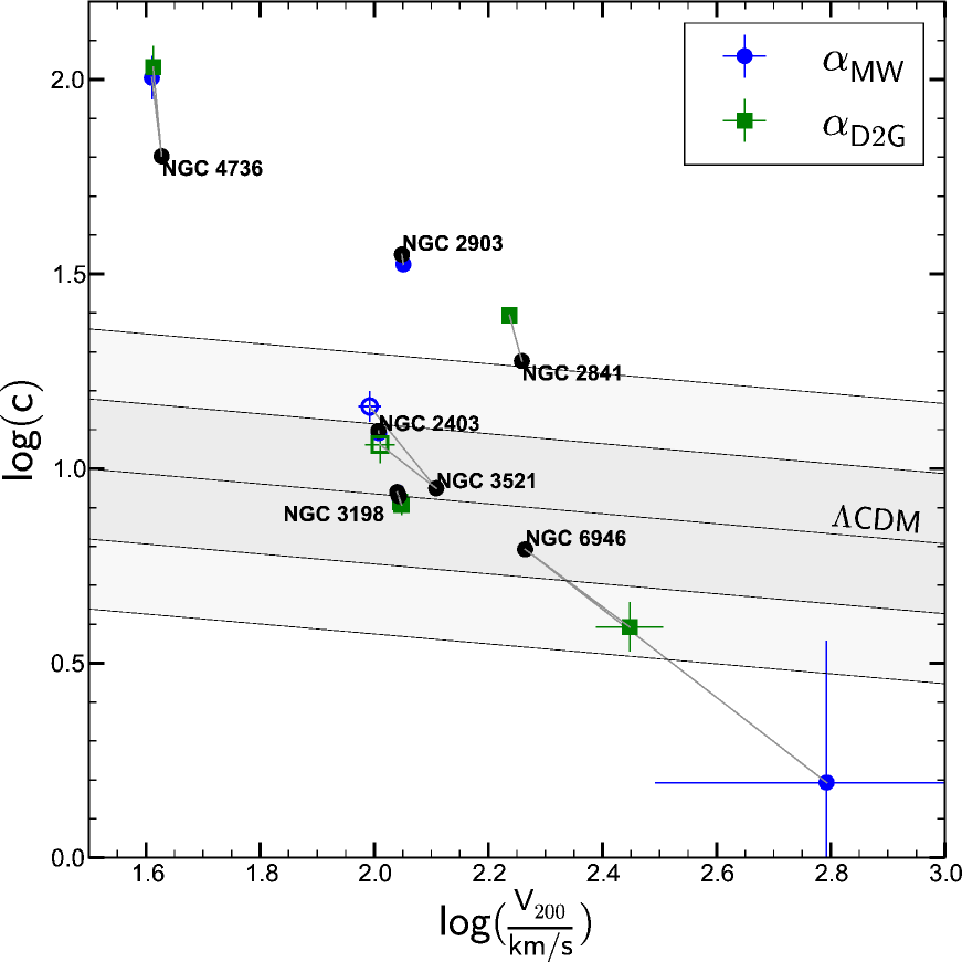
Figure 24.— Plot of fitted halo parameters for the NFW mass models, $\log\,(c)$ vs. $\log\,(V_{200}/\,\mathrm{km\,s^{-1}})$. Each point corresponds to the NFW model parameters that produces the lowest $\mathrm{\chi^{2}_{r}}$ value for each galaxy, for each value of $\alpha_{\mathrm{CO}}$. Green squares correspond to models where we use $\mathrm{\alpha_{D2G}}$; blue circles correspond to models where we use the Milky Way value. Filled symbols correspond to cases where the best fit was obtained with the THINGS rotation curve; unfilled symbols correspond to those with the HERACLES rotation curve. The H i-only values are plotted in black circles, and a line joins the H i-only value to the corresponding values calculated with added molecular gas, for each galaxy. The 1- and 2- component models are indicated for NGC 3198. We plot a line of expected values from $\mathrm{\Lambda CDM}$, bounded by $1\,\sigma$ and $2\,\sigma$ regions.

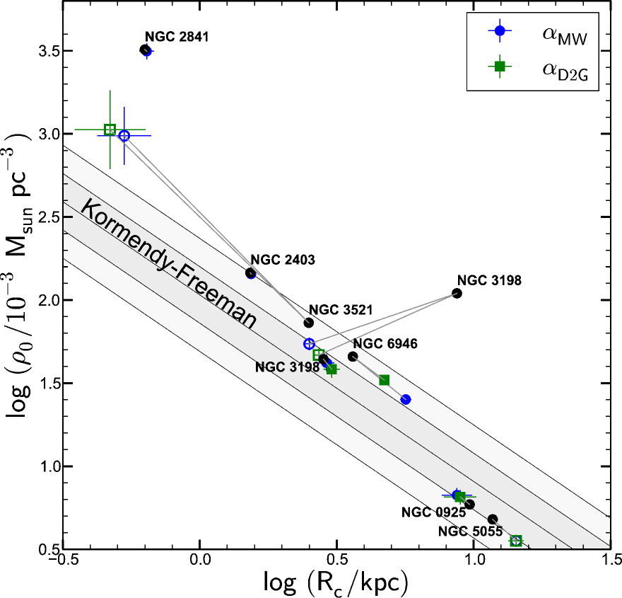
Figure 25.— Plot of fitted halo parameters for the ISO mass models, $\mathrm{\log(\rho_{0}/10^{-3}M_{\odot}\,pc^{-3})}$ vs. $\mathrm{\log{(R_{c}/\mathrm{\,kpc})}}$. Each point corresponds to the ISO model parameters that produces the lowest $\mathrm{\chi^{2}_{r}}$ value for each galaxy, for each value of $\alpha_{\mathrm{CO}}$. Symbols are as in Figure 24. The 1- and 2- component models are indicated for NGC 3198. We plot a line of expected values from Kormendy & Freeman (2004), bounded by $1\,\sigma$ and $2\,\sigma$ regions from Bullock et al. (2001)

Table 7 Fitted halo parameters for the NFW Model.

Galaxy	Rotcur	$\mathrm{\overline{\alpha}_{CO}}$	$c$	$V_{200}$	$\chi^{2}_{r}$	$c$	$V_{200}$	$\chi^{2}_{r}$
		($\frac{M_{\odot}\mathrm{\,pc^{-2}}}{\mathrm{K\,km\,s^{-1}}}$)		($\,\mathrm{km\,s^{-1}}$)			($\,\mathrm{km\,s^{-1}}$)
						H i only	H i only	H i only
NGC 2403 (1 comp)	H i	6.3	$12.2\pm 0.2$	$102.3\pm 0.7$	0.6	$12.4\pm 0.2$	$101.7\pm 0.7$	0.6
NGC 2403 (2 comp)	H i	6.3	$12.1\pm 0.2$	$102.3\pm 0.8$	0.6	$12.3\pm 0.2$	$102.2\pm 0.7$	0.6
NGC 2841	H i	6.3	$24.7\pm 0.4$	$172.7\pm 1.0$	0.6	$18.9\pm 0.4$	$181.4\pm 1.0$	0.2
NGC 2841	H i	7.1	$24.8\pm 0.4$	$172.6\pm 1.0$	0.6
NGC 3198 (1 comp)	COH i	6.3	$8.6\pm 0.4$	$109.7\pm 1.8$	1.5	$8.7\pm 0.4$	$109.7\pm 1.7$	1.3
NGC 3198 (1 comp)	H i	6.3	$8.3\pm 0.4$	$110.7\pm 1.8$	1.4
NGC 3198 (1 comp)	COH i	15.7	$8.3\pm 0.4$	$110.3\pm 1.8$	1.4
NGC 3198 (1 comp)	H i	15.7	$8.0\pm 0.4$	$111.3\pm 1.9$	1.4
NGC 3198 (2 comp)	COH i	6.3	$8.4\pm 0.5$	$110.5\pm 2.4$	2.5	$8.5\pm 0.5$	$110.4\pm 2.2$	2.1
NGC 3198 (2 comp)	H i	6.3	$8.2\pm 0.5$	$111.3\pm 2.4$	2.2
NGC 3198 (2 comp)	COH i	15.7	$8.1\pm 0.5$	$111.2\pm 2.5$	2.4
NGC 3198 (2 comp)	H i	15.7	$7.9\pm 0.5$	$112.0\pm 2.4$	2.1
NGC 3521	COH i	6.3	$14.5\pm 1.3$	$98.1\pm 4.5$	1.2	$8.9\pm 2.0$	$128.4\pm 16.4$	5.6
NGC 3521	H i	6.3	$6.4\pm 1.8$	$139.6\pm 24.2$	5.2
NGC 3521	COH i	10.9	$13.6\pm 1.3$	$98.5\pm 4.9$	1.3
NGC 3521	H i	10.9	$5.8\pm 1.8$	$143\pm 27$	5.1
NGC 4736	COH i	6.3	$54.8\pm 10.5$	$43.9\pm 2.0$	3.4	$63.5\pm 24.2$	$42.4\pm 1.7$	1.4
NGC 4736	H i	6.3	$91.9\pm 12.3$	$40.5\pm 1.0$	1.5
NGC 4736	COH i	1.4	$64.8\pm 11.6$	$44.0\pm 1.8$	3.5
NGC 4736	H i	1.4	$108.3\pm 13.7$	$40.9\pm 1.0$	1.5
NGC 6946	COH i	2.9	$3.4\pm 1.0$	$313.0\pm 84.3$	3.2	$6.2\pm 0.5$	$183.8\pm 11.1$	1.03
NGC 6946 (outer)	H i	2.9	$3.6\pm 0.6$	$296.2\pm 239.6$	1.2
NGC 7331 (outer)	H i	6.3	$4.0\pm 0.4$	$223.0\pm 14.1$	0.2	$4.9\pm 0.4$	$200.0\pm 10.7$	0.24

Table 8Fitted halo parameters for the ISO Model.

Galaxy	Rotcur	$\mathrm{\overline{\alpha}_{CO}}$	$R_{\mathrm{c}}$	$\rho_{0}$	$\chi^{2}_{r}$	$R_{\mathrm{c}}$	$\rho_{0}$	$\chi^{2}_{r}$
		($\frac{M_{\odot}\mathrm{\,pc^{-2}}}{\mathrm{K\,km\,s^{-1}}}$)	($\mathrm{\,kpc}$)	$\mathrm{(10^{-3}\,\,M_{\odot}\,pc^{-3})}$		($\mathrm{\,kpc}$)	$\mathrm{(10^{-3}\,\,M_{\odot}\,pc^{-3})}$
						H i only	H i only	H i only
NGC 0925	H i	6.3	$9.0\pm 1.3$	$6.4\pm 0.7$	1.5	$9.7\pm 1.3$	$5.9\pm 0.5$	1.1
NGC 0925	H i	14.3	$8.9\pm 1.2$	$6.5\pm 0.7$	1.5
NGC 2403 (1 comp)	H i	6.3	$1.5\pm 0.1$	$144.4\pm 7.1$	1.0	$1.49\pm 0.05$	$152.8\pm 7.5$	1.0
NGC 2403 (2 comp)	H i	6.3	$1.6\pm 0.1$	$138.0\pm 6.6$	1.0	$1.52\pm 0.04$	$145.8\pm 6.9$	1.0
NGC 2841	H i	6.3	$0.7\pm 0.1$	$3035\pm 335$	0.2	$0.63\pm 0.04$	$3215.3\pm 371.8$	0.2
NGC 2841	H i	7.1	$0.6\pm 0.1$	$3163\pm 358$	0.2
NGC 2976	H i	6.3	$4.1\pm 1.9$	$35.3\pm 4.0$	0.7	$5.1\pm 2.5$	$35.5\pm 3.1$	$0.5$
NGC 2976	H i	4.7	$2.6\pm 0.7$	$42.8\pm 4.9$	0.8
NGC 3198 (1 comp)	COH i	6.3	$2.7\pm 0.1$	$48.5\pm 4.3$	0.9	$2.7\pm 0.1$	$46.9\pm 4.0$	0.8
NGC 3198 (1 comp)	H i	6.3	$2.9\pm 0.2$	$42.2\pm 3.8$	0.9
NGC 3198 (1 comp)	COH i	15.7	$2.8\pm 0.1$	$45.2\pm 4.0$	0.9
NGC 3198 (1 comp)	H i	15.7	$3.0\pm 0.2$	$39.1\pm 3.5$	0.9
NGC 3198 (2 comp)	COH i	6.3	$2.8\pm 0.2$	$45.1\pm 5.5$	1.7	$2.8\pm 0.1$	$44.0\pm 5.1$	1.4
NGC 3198 (2 comp)	H i	6.3	$3.0\pm 0.2$	$39.7\pm 4.7$	1.5
NGC 3198 (2 comp)	COH i	15.7	$2.9\pm 0.3$	$41.9\pm 5.1$	1.7
NGC 3198 (2 comp)	H i	15.7	$3.1\pm 0.2$	$36.8\pm 4.3$	1.5
NGC 3521	COH i	6.3	$0.5\pm 0.1$	$973\pm 388$	1.0	$2.5\pm 0.7$	$73.0\pm 30.6$	4.8
NGC 3521	H i	6.3	$3.4\pm 0.9$	$39.0\pm 15.3$	4.7
NGC 3521	COH i	10.9	$0.5\pm 0.1$	$1024\pm 451$	1.1
NGC 3521	H i	10.9	$3.6\pm 1.0$	$33.4\pm 13.1$	4.6
NGC 5055	COH i	6.3	$18.6\pm 2.0$	$2.6\pm 0.3$	2.5	$11.7\pm 0.7$	$4.8\pm 0.4$	1.0
NGC 5055	H i	6.3	$18.6\pm 2.0$	$2.6\pm 0.3$	2.7
NGC 5055	COH i	5.3	$16.7\pm 1.4$	$3.0\pm 0.3$	1.8
NGC 5055	H i	5.3	$16.6\pm 1.5$	$3.1\pm 0.3$	1.9
NGC 6946	COH i	6.3	$7.8\pm 0.8$	$16.3\pm 1.7$	3.8	$3.6\pm 0.2$	$45.7\pm 3.0$	1.0
NGC 6946 (outer)	H i	6.3	$7.8\pm 0.5$	$16.4\pm 1.0$	1.3
NGC 6946	COH i	2.9	$4.8\pm 0.4$	$31.4\pm 3.0$	2.9
NGC 6946 (outer)	H i	2.9	$4.8\pm 0.2$	$31.4\pm 1.7$	0.9

Appendix A Velocity Fields and Tilted-ring Models

For each galaxy we present the IWM and $\mathrm{Her_{3}}$ velocity fields derived in dB08 and in this work. We plot the CO distribution overlaid on the SINGS $3.6\mu$m image. We plot major- and minor-axis pV diagrams, where we have used the position angle from the THINGS data to make the pV slices. We also plot the H i and CO TM and HM rotation curves. These are all plotted in Figures 26-37. Each plot is organized as follows:

Top Row. Left: H i IWM velocity field. The THINGS systemic velocity $V_{\mathrm{sys}}$ is plotted with a thick black contour, the approaching contours are plotted in white, receding contours are plotted in black. The velocity increments $\Delta V$ between contours are indicated in the figure caption. Centre: The H i $\mathrm{Her_{3}}$ velocity field contours are the same as for velocity field in the left panel. The colour bar on the right of this panel denotes the velocity spread for all the velocity fields in these plots in units of $\,\mathrm{km\,s^{-1}}$. Right: CO integrated surface brightness contours are plotted in red on top of the SINGS $3.6\mu$m image (greyscale); the contour levels are generally given by $I_{\mathrm{CO}}=I_{0},I_{0}+\Delta I,...\,\mathrm{K}\,\,\mathrm{km\,s^{-1}}$ where $I_{0}$ and $\Delta I$ are denoted in the caption. For some galaxies (e.g., NGC 2903) levels are given by $I_{\mathrm{CO}}=2^{N}\,\mathrm{K}\,\,\mathrm{km\,s^{-1}}$ where the values of $N$ are denoted in the figure caption. The CO and $3.6\mu$m levels are denoted in each caption.

Middle Row. Left: CO IWM velocity field. The systemic velocity $V_{\mathrm{sys}}$ is plotted with a thick black contour, the approaching contours are plotted in white, receding contours are plotted in black. The velocity increments $\Delta V$ are indicated in the figure caption. Middle: CO $\mathrm{Her_{3}}$ velocity field which was used to calculate the tilted-ring models, contours are the same as for velocity field in the left panel. Right: Difference velocity field, showing the difference between the H i and CO $\mathrm{Her_{3}}$ velocity field. The velocity colour scale corresponds to the colour bar to the left of this panel in units of $\,\mathrm{km\,s^{-1}}$. Black contours correspond to $\pm 5\,\mathrm{km\,s^{-1}}$, thicker dark grey contours correspond to $\pm 10\,\mathrm{km\,s^{-1}}$.

Bottom Row. Left: Position velocity (pV) major-axis diagram; the H i is plotted in filled contours from $\sigma_{\mathrm{HI}}$ upwards in multiples of $\sigma_{\mathrm{HI}}$ and the CO is plotted in red contours from $\sigma_{\mathrm{CO^{\prime}}}$ upwards in multiples of $\sigma_{\mathrm{CO^{\prime}}}$. These values are tabulated in Table 2. The major-axis position angle is indicated in the panel title. Middle: pV minor-axis diagram. Right: Rotation curves presented in this work. The H i rotation curves derived in dB08 are plotted in red unfilled circles. For galaxies where we only calculate TM rotation curves, we plot the CO rotation curve in filled dark-grey squares with error-bars. For galaxies where we calculate TM and HM rotation curves, we plot the TM rotation curves in unfilled light-grey squares, and we plot the HM rotation curves in filled black circles with errorbars.

A.1. NGC 925

NGC 925 is an SABd galaxy, and shows the least CO emission of the sample galaxies. In Figure 26 we plot the H i and CO velocity fields and the pV diagrams. We see that the CO is concentrated along the approaching side of the galaxy. The CO emission is insufficient to constrain an independent model. We therefore use the TM to compute the rotation curve, which is plotted in Figure 4. The CO rotation curve is lower than the H i rotation curve. This is due to the lopsided emission of the CO, which introduces a bias towards the approaching side when computing the rotation curve. This can be seen for the THINGS rotation curve in dB08, where it is shown that the rotation curve on the approaching side is lower than the total rotation curve within a radius of $\sim 80^{\prime\prime}$.

A.2. NGC 2403

NGC 2403 is a late-type SABcd galaxy, and its H i emission has been studied extensively, e.g., early observations by Shostak & Rogstad (1973), more recent observations include Fraternali et al. (2002). Sofue (1997) used the observations from Thornley & Wilson (1995) to derive the CO rotation curve using the envelope tracing method.

In Figure 27 we present the velocity fields and pV diagrams of the H i and CO distributions of NGC 2403. The CO emission is patchy and the pV diagrams show a good correspondence between the H i and CO emission. The CO emission is sufficient to calculate an independent HM rotation curve, which we plot in Figure 5. The H i and CO rotation curves are in good agreement, and only show slight differences for the very inner radius.

A.3. NGC 2841

NGC 2841 is an SAb galaxy. In Figure 28 we plot the velocity fields and pV diagrams for the H i and CO data. The H i shows a hole in the centre, which we also observe in the CO. We see a good correspondence between the H i and the CO in the pV diagrams. The CO emission is not sufficient to constrain an independent tilted-ring model, so we compute the rotation curve using the TM. The rotation curve is plotted in Figure 4.

A.4. NGC 2903

NGC 2903 is an SABbc type galaxy. The BIMA-SONG (Helfer et al. 2003) observations show that the CO $J=1\rightarrow 0$ emission is concentrated along a molecular bar. NGC 2903 has also been observed as part of the survey described in Kuno et al. (2007). There is an excellent correspondence between the major-axis pV diagram and the velocity field presented therein, with those presented in this work.

In Figure 29 we plot the velocity fields and pV diagrams of the H i and CO data. The CO/$3.6\mu$m overlay shows that the CO $J=2\rightarrow 1$ emission is concentrated along a bar. There is also low surface density CO across the disk of the galaxy. The kinks in the iso-velocity contours in the CO velocity fields are indicative of the non-circular streaming motions which dominate in the central regions. The difference velocity field shows a large difference, indicating that the H i is not sensitive to the small scale bar perturbations. This is also noted in Sellwood & Sánchez (2010), who found the H$\alpha$ to be a more reliable tracer of the bar than the H i data.

The presence of the bar makes it difficult to compute an independent HM model. We therefore use the TM with the understanding that the inner parts (within $\sim 100^{\prime\prime}$) of the CO rotation curve is dominated by non-circular motions, and therefore cannot be used to trace the rotational velocity of the galaxy. The final rotation curve is plotted in Figure 4.

A.5. NGC 2976

NGC 2976 is an SAc galaxy. Simon et al. (2003) obtained CO $J=1\rightarrow 0$ observations of NGC 2976 using the BIMA array. In Figure 30 we plot the CO and H i velocity fields, pV diagrams, rotation curves and the CO distribution overlaid on the associated SINGS map. The CO distribution is almost as extended as the H i. The pV diagrams show a good agreement between the H i and the CO. The distribution of the CO is sufficient to calculate an independent HM model. The HM and TM rotation curve is plotted in Figure 5.

Simon et al. (2003) show that the CO $J=1\rightarrow 0$ surface density falls off rapidly at about $40^{\prime\prime}$ away from the centre of the galaxy. They therefore use their $\mathrm{H}\alpha$ data to determine the rotation curve out to the edge of the disk. Our rotation curve is in good agreement with their hybrid rotation curve; their $\mathrm{H}\alpha$ rotation curve also tracks the deviation from a linear rise at approximately $60^{\prime\prime}$.

Spekkens & Sellwood (2007) perform an analysis of the non-circular motions in NGC 2976 using their package VELFIT, which includes the $m=1$ and $m=2$ modes in an explicit fit to the entire velocity field (as opposed to the radially independent tilted-ring model). They fit an $m=2$ (as due to a bar) Fourier mode to the CO $J=1\rightarrow 0$ velocity field from Simon et al. (2003). They show that the deviation in the CO rotation curve from a linear rise at approximately $60^{\prime\prime}$ is principally due to the bar-streaming motion. It additionally seems likely that the $m=2$ radial and tangential variations are responsible for the fact that the CO rotation curve is consistently lower than the THINGS rotation curve.

A.6. NGC 3198

NGC 3198 is an SBc type galaxy. In Figure 31 we plot the velocity fields derived in this work. The velocity fields show the paucity of the CO emission. The difference velocity field in Figure shows that the H i and CO velocity fields are in good agreement. The major-axis pV diagram shows a good correspondence between the CO and the H i, while the minor-axis pV diagram shows possible kinematic evidence for streaming motions, which can be associated with the weak bar (Bottema et al. 2002). The CO emission is sufficient for us to compute an HM model, which we plot in Figure 5.

While the CO and H i tilted-ring models are in generally good agreement, we note two large differences between the CO and H i rotation curves. The first difference is at approximately $30^{\prime\prime}$. The second is at approximately $90^{\prime\prime}$. The difference at $30^{\prime\prime}$ can be related to the presence of a weak bar. The effect of a bar was noted by Bottema et al. (2002), who speculate that the bar would be oriented parallel to the line of sight (aligned with the observed minor-axis) based on the $\mathrm{H}\alpha$ morphology. They use the results of Teuben & Sanders (1985) to provide a qualitative interpretation of the effect of the bar - which is to increase the apparent rotational velocity within $30^{\prime\prime}$. This is consistent with our results. The difference at $90^{\prime\prime}$ can be related to the low-filling factor of the CO at these radii. The filling factor drops to less than $5\%$ beyond $\sim 100^{\prime\prime}$.

A.7. NGC 3521

NGC 3521 is an SABbc galaxy, and has also been been observed as part of the Kuno et al. (2007) survey. Their results also show a depletion of CO in the centre of the galaxy. The comparison of the H i and CO velocity fields are shown in Figure 32. The H i-CO difference velocity field is large in the inner part of the galaxy, which corresponds to the difference in the pV diagrams for both components. This corresponds to the warp in the H i distribution, along the line of sight, which affects the derived velocity field.

We derive an HM rotation curve from the CO data. This is plotted in Figure 5. The CO rotation curve is higher than the H i within $\sim 60^{\prime\prime}$ - the CO rotation curve is almost 50$\,\mathrm{km\,s^{-1}}$ higher than the H i rotation curve for the innermost four points. It is likely that the H i velocities at these radii are affected by the presence of emission due to the warp in the line of sight.

A.8. NGC 3627

NGC 3627 is an SABb galaxy and is part of the Leo Triplet. Notable studies of the molecular gas content of NGC 3627 are Young et al. (1983) and Kuno et al. (2007). Studies of the kinematics of the ionized gas (Chemin et al. 2003) and the H i (Trachternach et al. 2008) show strong signs of non-circular motions, which are due to the bar streaming motions as well as tidal interactions within the group.

The comparison of the H i and CO data is shown in Figure 33. The HERACLES data shows that the CO distribution is lopsided and although the CO velocity fields shows a general velocity gradient, the iso-velocity contours and the pV diagram show signs of non-circular motions. The H i-CO difference velocity field shows large differences in the centre of the galaxy, where the H i distribution shows signs of a depression.

The presence of several different sources of perturbations which could lead to non-circular motions makes it difficult to determine a tilted-ring model for the CO data. We therefore use the THINGS parameters to calculate the rotation curve. For the inner part of NGC 3627 we assume the inclination and position angle of the inner most tilted-ring from the THINGS data. The rotation curve plotted in Figures 4 and 33 show a good agreement between the H i and the CO from a radius of approximately $50^{\prime\prime}$ outwards. Due to the complex kinematics of the H i and CO, we do not use the data for NGC 3627 to fit mass models.

A.9. NGC 4736

NGC 4736 is an SAab galaxy. NGC 4736 has a compact molecular component. This can be see as the excess emission near systemic velocity in the CO line profile (see Figure 1) and the minor axis pV diagram. The velocity fields and the pV diagram which are plotted in Figure 34. NGC 4736 has also been observed as part of the survey described in Kuno et al. (2007). We note a good agreement between the pV diagram and velocity field presented therein, and those presented in this work. There is no systematic difference between the H i and CO velocity fields in the region where they overlap. The tilted-ring parameters used to compute the CO rotation curve were extrapolated from the TM by assuming a constant value inwards from the innermost point, since there is a central depression of H i. It was not possible to compute an independent HM model because of the low inclination. We plot the rotation curve in Figure 4.

Wong & Blitz (2000) did a thorough investigation of the non-circular kinematics in NGC 4736, solving for inflow and outflow models. Their rotation curve shows the same features as ours, but the velocity that they find at the first maximum is higher than ours by approximately $20\,\mathrm{km\,s^{-1}}$. Haan et al. (2009) studied NGC 4736 as part of a search for gas radial flows, which was based on the NUGA survey. They used high-resolution observations of the $J=2\rightarrow 1$ and $J=1\rightarrow 0$ transitions of CO to map the central molecular component. Their rotation curve rises to $200\,\mathrm{km\,s^{-1}}$ within $0.3\mathrm{\,kpc}$, which corresponds to a single beam of the HERACLES survey. The rotation curve that we derive rises steeply (within $0.5\mathrm{\,kpc}$), but the rise is not as steep as the rotation curve derived by Haan et al. (2009), which could be due to differences in the beam sizes, since the synthesized beam of the Plateau du Bure is approximately $0.5^{\prime\prime}$.

A.10. NGC 5055

NGC 5055 is an SAbc galaxy with extended CO emission across the optical disk. The H i and CO profiles are in good agreement with each other (Figure 1).

Thornley & Mundy (1997) studied the morphology and kinematics of NGC 5055 in CO. NGC 5055 has also been observed as part of the Kuno et al. (2007) survey. We note a good agreement between the pV diagram and velocity field presented therein, and those presented in this work. In Figure 35 we plot the H i and CO velocity fields and pV diagrams for NGC 5055. The velocity fields appear to be in good agreement, and the difference velocity field shows small amplitudes. The large difference in the centre of the galaxy is due to a combination of differential beam smearing (the THINGS and HERACLES beamsizes are slightly different) and the difference in morphology between the H i and the CO.

The major-axis pV diagram shows that the H i and CO distributions are quite similar - we can thus expect that the H i and CO rotation curves show similar features.

The CO distribution is sufficient to compute an independent HM rotation curve. The rotation curves for NGC 5055 are plotted in Figure 5. We also note that Wong et al. (2004) studied CO and H i data for NGC 5055; the CO rotation curve derived in their work (computed from the BIMA-SONG data) goes out to approximately $100^{\prime\prime}$, and is sufficient to trace the rising part of the rotation curve.

The H i and CO rotation curves are in good agreement with each other, with the CO rotation velocities being slightly higher (the differences are within the error-bars and certainly less than about $5\,\mathrm{km\,s^{-1}}$) than that for the H i within $100^{\prime\prime}$.

A.11. NGC 6946

NGC 6946 is an SABcd galaxy and has historically been a popular target for CO observations (Young & Scoville 1982; Ball et al. 1985; Tosi & Diaz 1985; Sofue et al. 1988; Tacconi & Young 1989; Casoli et al. 1990; Israel & Baas 2001; Meier & Turner 2004; Schinnerer et al. 2006; Crosthwaite & Turner 2007). The CO morphology includes a bright nuclear structure and fainter spiral arms. The nuclear structure was the object of several detailed studies (Ball et al. 1985; Casoli et al. 1990; Schinnerer et al. 2006). There are various studies comparing the distribution and kinematics of different molecules, e.g., different transitions of CO, as in Israel & Baas (2001). NGC 6946 has also been observed as part of the Kuno et al. (2007) survey. We note a good agreement between the pV diagram and velocity field presented therein, and those presented in this work. In Figure 36 we plot the H i and CO velocity fields.

The low inclination of the CO emission is at the limit of what can be modelled using a tilted-ring model. We therefore use the TM as the estimate of the kinematics, and we compute the rotation curve, which is plotted in Figure 4.

Schinnerer et al. (2006) derived rotation curves from high resolution Plateau de Bure interferometer observations of CO $J=1\rightarrow 0$ and CO $J=2\rightarrow 1$ in a manner very similar to that used in this work, i.e., velocity field fitting using a tilted-ring model in ROTCUR. Their rotation curves show a rapid rise to approximately $150\,\mathrm{km\,s^{-1}}$ within $10^{\prime\prime}$, which is well within a single beam of our observations. Even at $13^{\prime\prime}$ (the resolution of HERACLES), our rotation curve predicts a rotational velocity $<100\,\mathrm{km\,s^{-1}}$, and only reaches $150\,\mathrm{km\,s^{-1}}$ at a radius of approximately $100^{\prime\prime}$. Schinnerer et al. (2006) attribute the steep rise in the rotation curve to the response of the gas to the inner nuclear bar, which is unresolved in the HERACLES observations.

A.12. NGC 7331

NGC 7331 is an SAb galaxy. In Figure 37 we plot the H i and CO velocity fields and pV diagrams. The H i is distributed in a disk with a central depression. The CO emission is distributed across the extent of the optical disk and overlaps with the H i emission. The CO emission is sufficient to compute an HM rotation curve, which is plotted in Figure 5.

von Linden et al. (1996) performed an in-depth analysis of NGC 7331, which included simulations of the evolution of the spiral structure of the galaxy. They derive CO $J=2\rightarrow 1$ and $J=1\rightarrow 0$ rotation curves, which are not inclination corrected. The shape of their rotation curve is consistent with the one derived in this work. They consider the velocities derived in their rotation curve as being lower than the real maximum velocity of the galaxy, due to the presence of molecular gas along the line of sight. The tilted-ring model explicitly accounts for the disk geometry, and our maximum velocity ($\sim 260\,\mathrm{km\,s^{-1}}$) is indeed higher than their associated inclination corrected maximum velocity $\sim 230\,\mathrm{km\,s^{-1}}$.

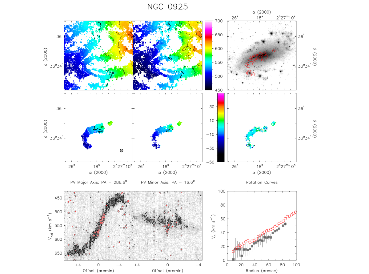
Figure 26.— Multi-panel plots for NGC 925. See the Appendix for a description of each panel. $V_{\mathrm{sys}}=546.3\,\mathrm{km\,s^{-1}}$, $\Delta V=25\,\mathrm{km\,s^{-1}}$. SINGS $3.6\mu$m grayscale image: $0.1\times 2^{N}$ MJy/sr, $N=0,0.2,...,4$; CO Moment-0 contours: 0 to 4 K$\,\,\mathrm{km\,s^{-1}}$ in stpdf of 1 K$\,\,\mathrm{km\,s^{-1}}$.

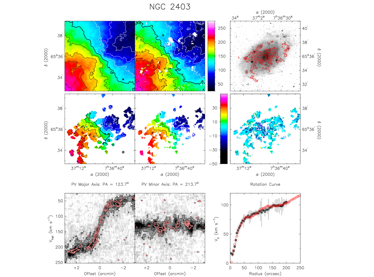
Figure 27.— Multi-panel plots for NGC 2403. See the Appendix for a description of each panel. $V_{\mathrm{sys}}=132.8\,\mathrm{km\,s^{-1}}$, $\Delta V=25\,\mathrm{km\,s^{-1}}$. SINGS $3.6\mu$m grayscale image: $0.1\times 2^{N}$ MJy/sr, $N=0,0.5,...,5.0$; CO Moment-0 contours: 0, 1.5 and 3 K$\,\,\mathrm{km\,s^{-1}}$.

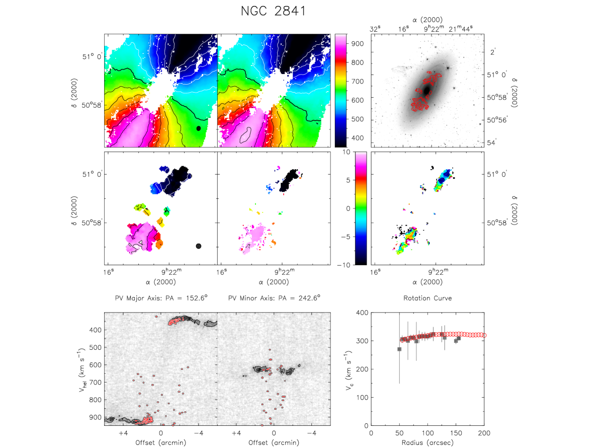
Figure 28.— Multi-panel plots for NGC 2841. See the Appendix for a description of each panel. $V_{\mathrm{sys}}=632.7\,\mathrm{km\,s^{-1}}$, $\Delta V=50\,\mathrm{km\,s^{-1}}$. SINGS $3.6\mu$m grayscale image: $0.1\times 2^{N}$ MJy/sr, $N=0,0.1,...,6.0$; CO Moment-0 contours: 0, 2 and 4 K$\,\,\mathrm{km\,s^{-1}}$.

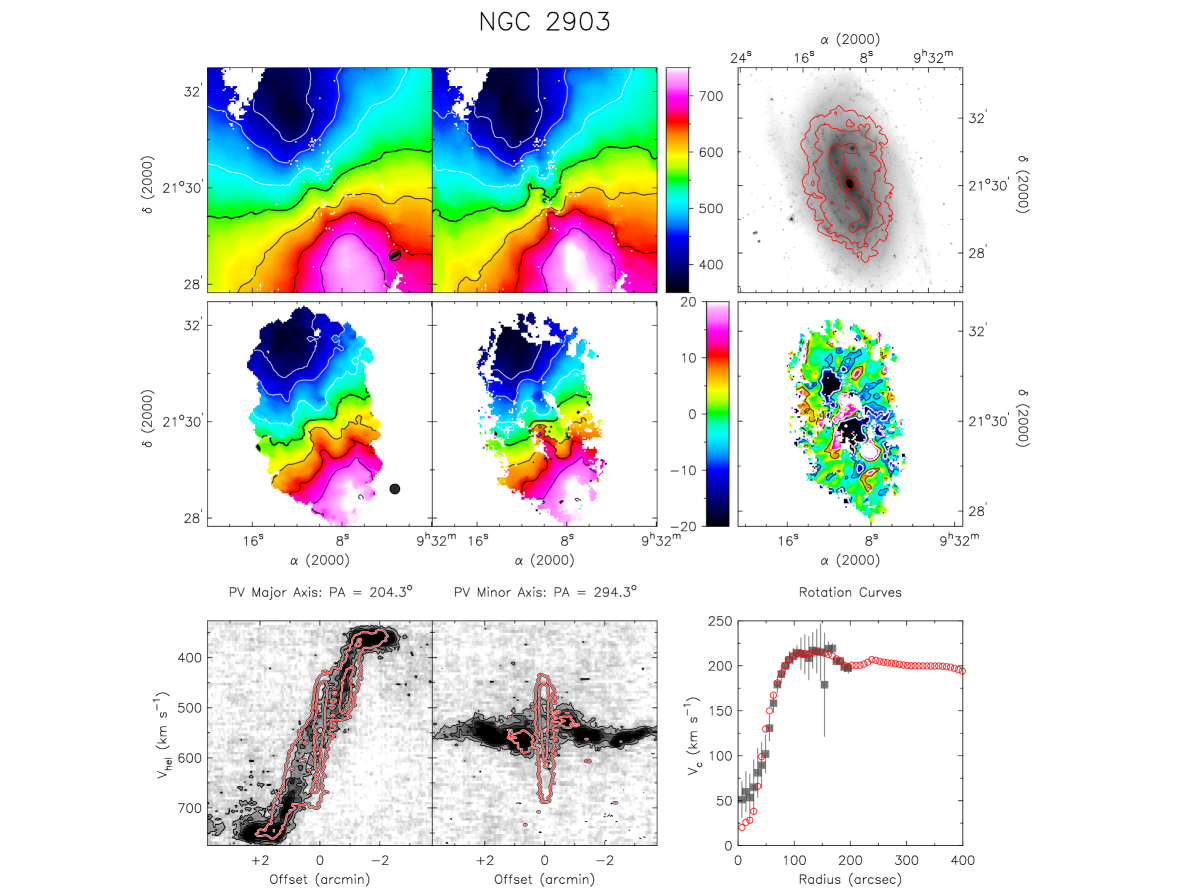
Figure 29.— Multi-panel plots for NGC 2903. See the Appendix for a description of each panel. $V_{\mathrm{sys}}=555.6\,\mathrm{km\,s^{-1}}$,, $\Delta V=40\,\mathrm{km\,s^{-1}}$. SINGS $3.6\mu$m grayscale image: $0.1\times 2^{N}$ MJy/sr, $N=0,0.1,...,8.0$; CO Moment-0 contours: $2^{N}$ K$\,\,\mathrm{km\,s^{-1}}$, $N=0,2,...20$. pV major- and minor-axis diagrams: H i contours are as designated in the appendix, the CO contours are $\sigma_{\mathrm{CO^{\prime}}}\times 2^{N}$ K$\,\,\mathrm{km\,s^{-1}}$, $N=0,2,...,10$.

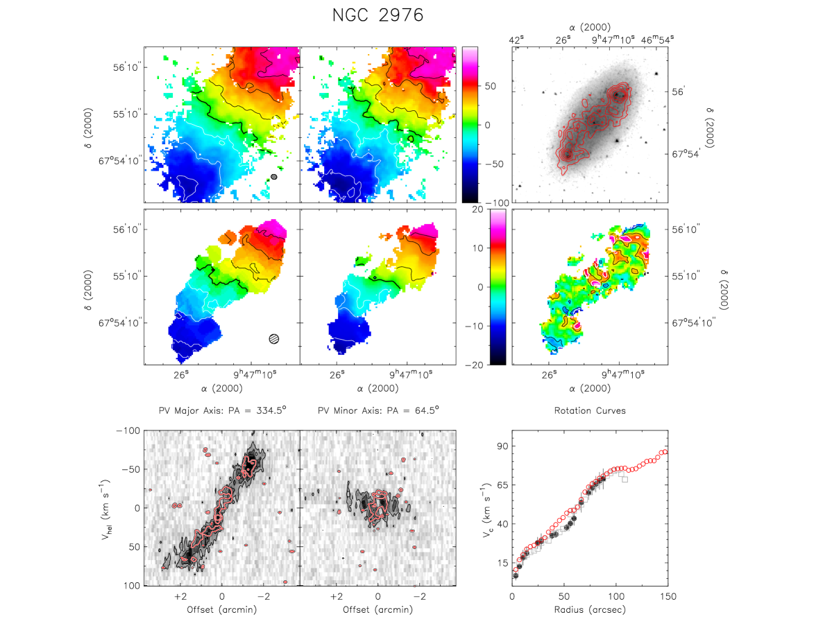
Figure 30.— Multi-panel plots for NGC 2976. See the Appendix for a description of each panel. $V_{\mathrm{sys}}=1.1\,\mathrm{km\,s^{-1}}$, $\Delta V=20\,\mathrm{km\,s^{-1}}$. SINGS $3.6\mu$m grayscale image: $0.1\times 2^{N}$ MJy/sr, $N=0,0.1,...,6.0$; CO Moment-0 contours: 1.6,3.2,…,8.0 K$\,\,\mathrm{km\,s^{-1}}$.

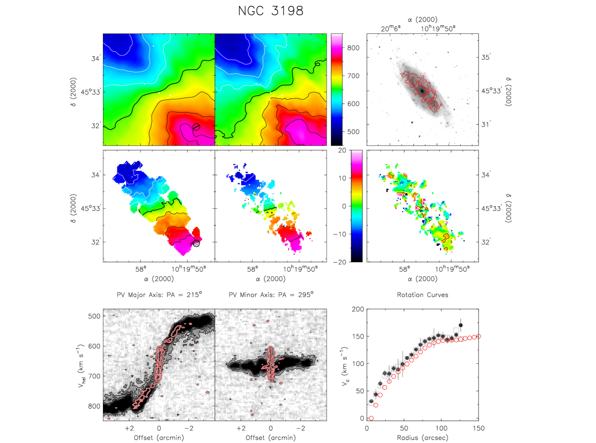
Figure 31.— Multi-panel plots for NGC 3198. See the Appendix for a description of each panel. $V_{\mathrm{sys}}=660.7\,\mathrm{km\,s^{-1}}$, $\Delta V=40\,\mathrm{km\,s^{-1}}$. SINGS $3.6\mu$m grayscale image: $0.1\times 2^{N}$ MJy/sr, $N=0,0.1,...,6.0$; CO Moment-0 contours: 1.5 and 3.0 K$\,\,\mathrm{km\,s^{-1}}$.

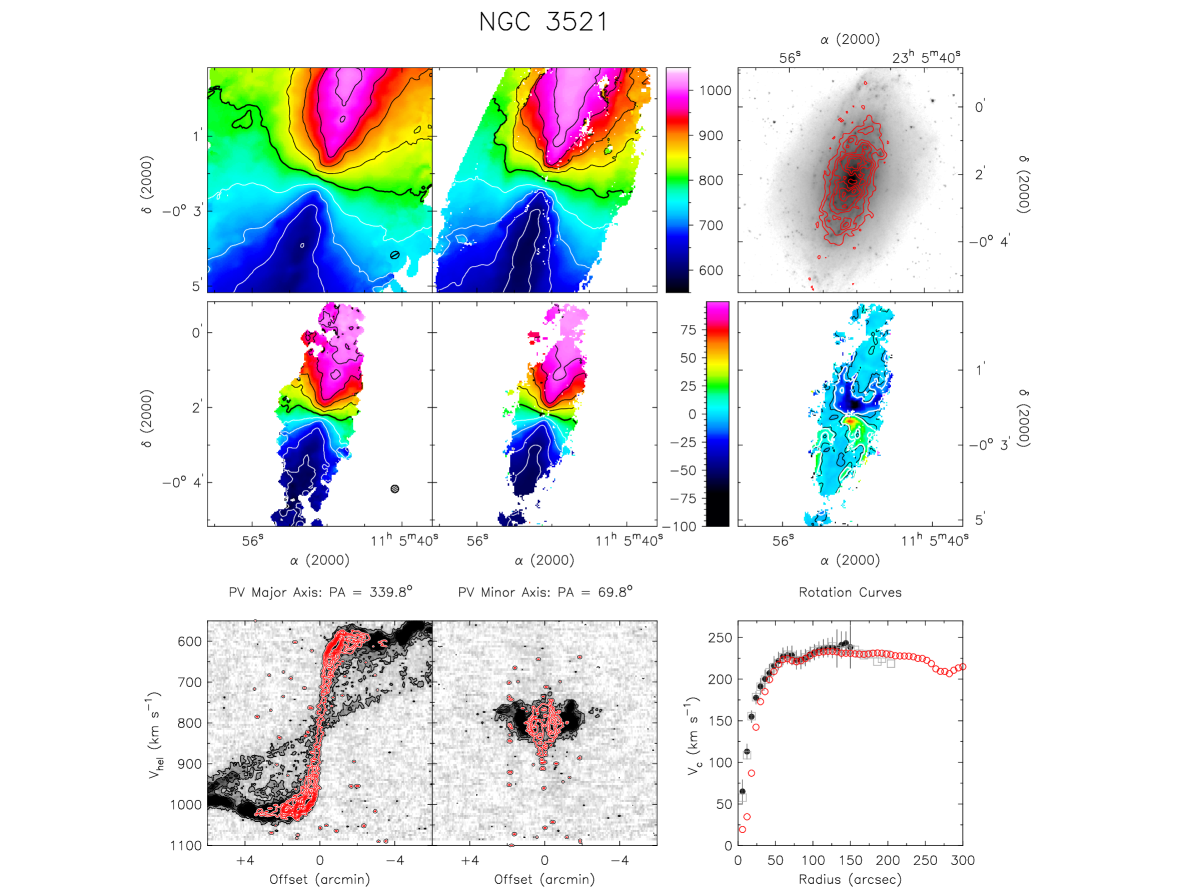
Figure 32.— Multi-panel plots for NGC 3521. See the Appendix for a description of each panel. $V_{\mathrm{sys}}=803.5\,\mathrm{km\,s^{-1}}$, $\Delta V=50\,\mathrm{km\,s^{-1}}$. SINGS $3.6\mu$m grayscale image: $0.1\times 2^{N}$ MJy/sr, $N=0,0.1,...,8.0$; CO Moment-0 contours: 5,10,…,35 K$\,\,\mathrm{km\,s^{-1}}$.

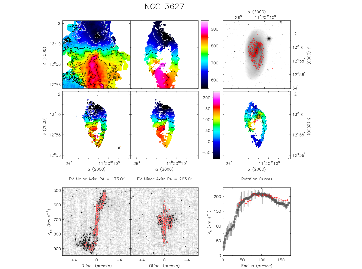
Figure 33.— Multi-panel plots for NGC 3627. See the Appendix for a description of each panel. $V_{\mathrm{sys}}=708.2\,\mathrm{km\,s^{-1}}$, $\Delta V=50\,\mathrm{km\,s^{-1}}$. SINGS $3.6\mu$m grayscale image: $0.1\times 2^{N}$ MJy/sr, $N=0,0.1,...,8.0$; CO Moment-0 contours: $1\,\mathrm{K}\,\,\mathrm{km\,s^{-1}}$ to $15\,\mathrm{K}\,\,\mathrm{km\,s^{-1}}$ in stpdf of $1.5\,\mathrm{K}\,\,\mathrm{km\,s^{-1}}$

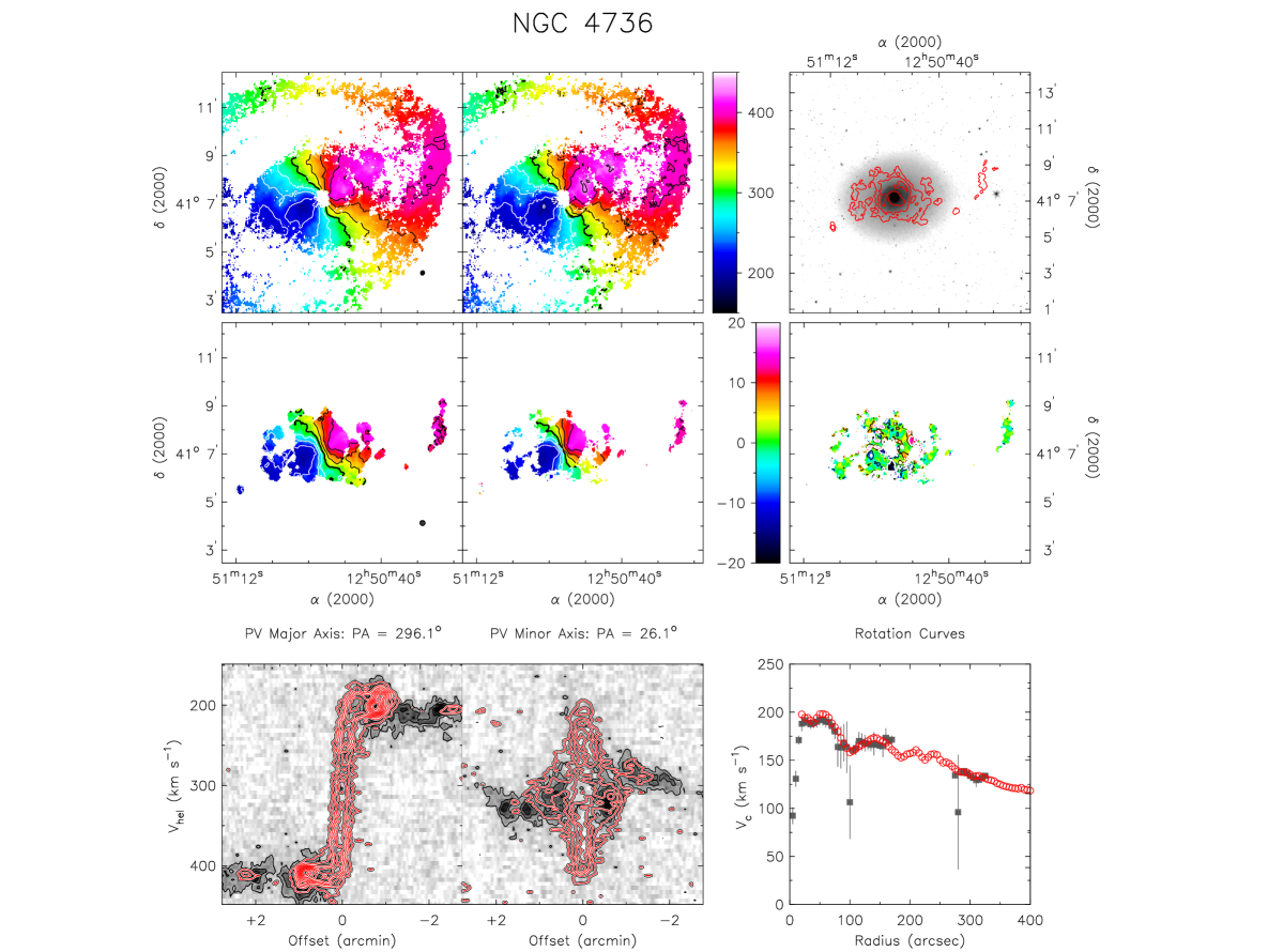
Figure 34.— Multi-panel plots for NGC 4736. See the Appendix for a description of each panel. $V_{\mathrm{sys}}=306.7\,\mathrm{km\,s^{-1}}$, $\Delta V=30\,\mathrm{km\,s^{-1}}$. SINGS $3.6\mu$m grayscale image: $0.1\times 2^{N}$ MJy/sr, $N=0,0.1,...,8.0$; CO Moment-0 contours: $2^{N}$ K$\,\,\mathrm{km\,s^{-1}}$, $N=0,2,...,10$.

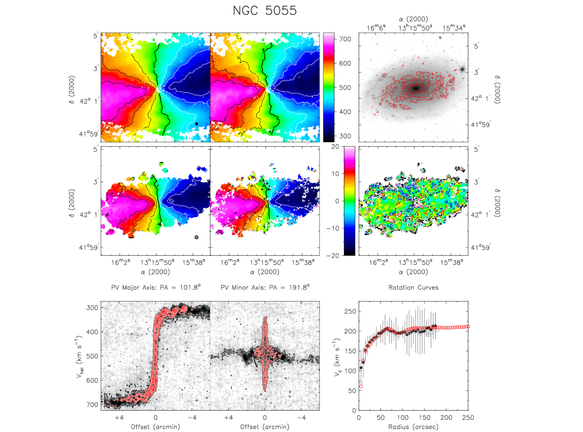
Figure 35.— Multi-panel plots for NGC 5055. See the Appendix for a description of each panel. $V_{\mathrm{sys}}=496.8\,\mathrm{km\,s^{-1}}$, $\Delta V=50\,\mathrm{km\,s^{-1}}$. SINGS $3.6\mu$m grayscale image: $0.1\times 2^{N}$ MJy/sr, $N=0,0.1,...,8.0$; CO Moment-0 contours: 5,10,…,35 K$\,\,\mathrm{km\,s^{-1}}$.

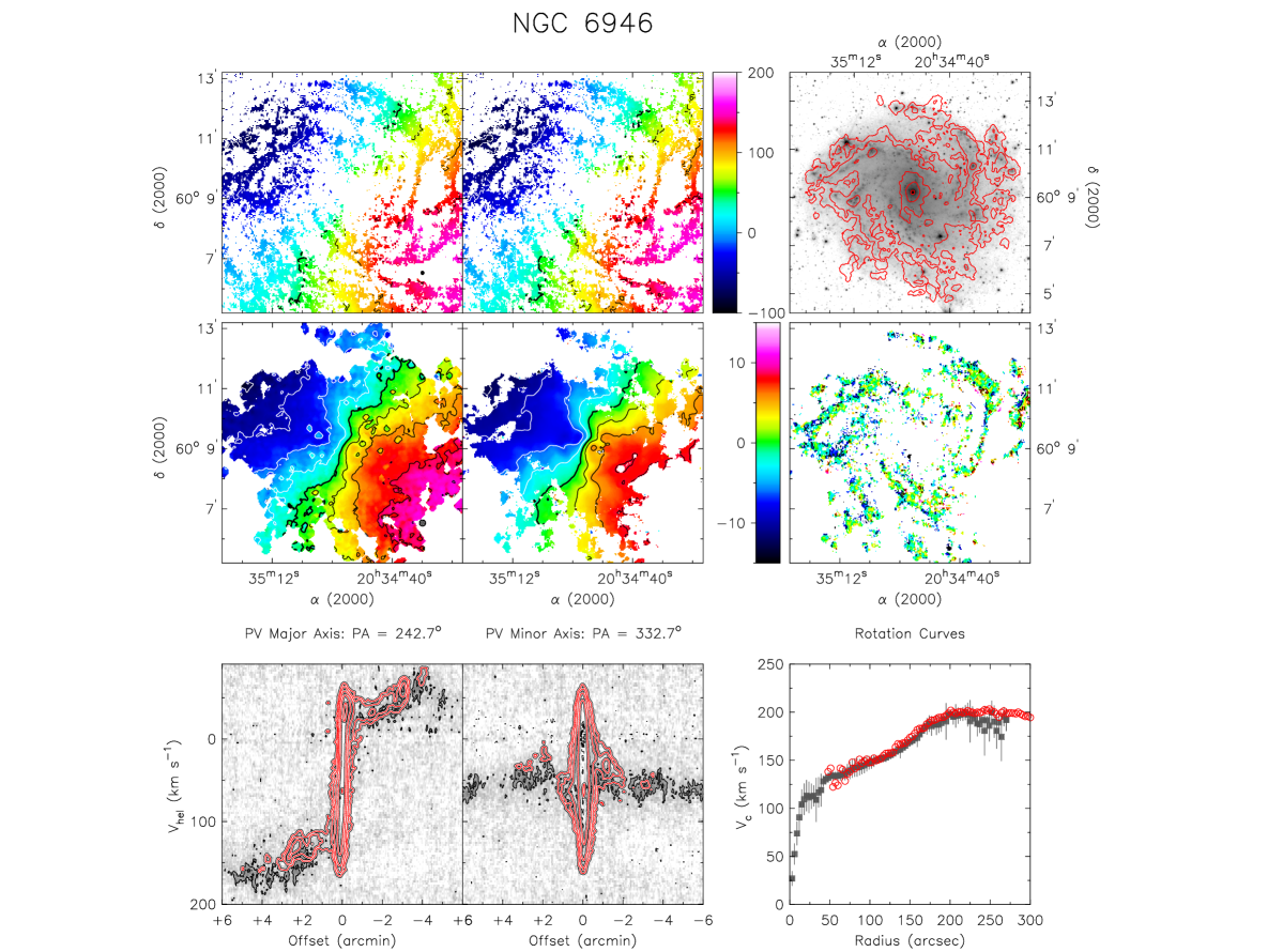
Figure 36.— Multi-panel plots for NGC 6946. See the Appendix for a description of each panel. $V_{\mathrm{sys}}=43.7\,\mathrm{km\,s^{-1}}$, $\Delta V=30\,\mathrm{km\,s^{-1}}$. SINGS $3.6\mu$m grayscale image: $0.1\times 2^{N}$ MJy/sr, $N=0,0.1,...,8.0$; CO Moment-0 contours: $2^{N}$ K$\,\,\mathrm{km\,s^{-1}}$, $N=0,2,...,10$.

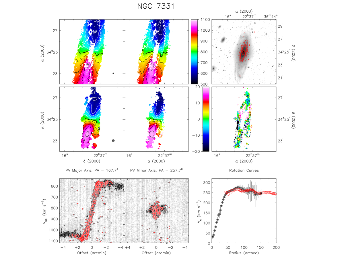
Figure 37.— Multi-panel plots for NGC 7331. See the Appendix for a description of each panel. $V_{\mathrm{sys}}=818.3\,\mathrm{km\,s^{-1}}$, $\Delta V=30\,\mathrm{km\,s^{-1}}$. SINGS $3.6\mu$m grayscale image: $0.1\times 2^{N}$ MJy/sr, $N=0,0.1,...,8.0$; CO Moment-0 contours: 5, 10, 15 and 20 K$\,\,\mathrm{km\,s^{-1}}$.

Appendix B Fitting Analytic Expressions to the Rotation Curves

Following Leroy et al. (2008) we fit the analytic expression described in Boissier et al. (2003):

$$v_{\mathrm{rot}}(r)=v_{\mathrm{flat}}\Bigg{[}1-\exp\big{(}\frac{-r}{l_{\mathrm{flat}}}\big{)}\Bigg{]}$$ (B1)

where $v_{\mathrm{rot}}$ is the circular velocity at radius $r$ (the rotation curve) and $v_{\mathrm{flat}}$ and $l_{\mathrm{flat}}$ are parameters corresponding to the velocity and the scale length at which the rotation curve approaches flatness, respectively. We use a non-linear least-square algorithm to fit the analytic rotation curves to the CO rotation curves presented in this work. The corresponding best fit values for $v_{\mathrm{flat}}$ and $l_{\mathrm{flat}}$ are presented in Table 9. In Figure 38 we plot the best fit model rotation curves and the observed CO rotation curves derived using the THINGS Model. We do not include the results for NGC 4736, since the analytic model cannot fit a declining rotation curve, by definition. We find that the $v_{\mathrm{flat}}$ are similar for fits to the CO and H i rotation curves, while the values of $l_{\mathrm{flat}}$ are slightly lower when fit to the CO rotation curves.

Table 9Fitted parameters of the Boissier et al. (2003) analytic rotation curve to the CO and H i rotation curves, $v_{\mathrm{flat}}$ and $l_{\mathrm{flat}}$. The parameters for the H i are as in Leroy et al. (2008).

Galaxy	$v_{\mathrm{flat}}$	$l_{\mathrm{flat}}$
	($\,\mathrm{km\,s^{-1}}$)	($\mathrm{\,kpc}$)
NGC 2403	97	0.5
NGC 2841	310	0.1
NGC 2903	210	1.6
NGC 2976	305	6.1
NGC 3198	152	2.5
NGC 3521	231	0.9
NGC 3627	88.8	0.9
NGC 5055	197	0.6
NGC 6946	182	1.4
NGC 7331	286	0.5
HERACLES Model
NGC 2403	98	0.6
NGC 2976	139	2.5
NGC 3198	159	2.7
NGC 3521	233	0.9
NGC 5055	197	0.6
NGC 7331	286	0.5

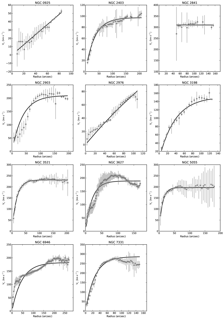
Figure 38.— CO rotation curves (using the THINGS-Model) with the fitted analytic rotation curves described in Boissier et al. (2003). The CO rotation curves are plotted as filled grey squares with error bars; The Boissier fits are plotted as solid black lines. The fits for NGC 4736 are not included here, since the Boissier et al. (2003) curves cannot fit a declining rotation curve.

References

- Ball et al. (1985) Ball, R., Sargent, A. I., Scoville, N. Z., Lo, K. Y., & Scott, S. L. 1985, ApJ, 298, L21
- Begeman (1989) Begeman, K. G. 1989, A&A, 47
- Bell & de Jong (2001) Bell, E. F. & de Jong, R. S. 2001, ApJ, 550, 212
- Boissier et al. (2003) Boissier, S., Prantzos, N., Boselli, A., & Gavazzi, G. 2003, MNRAS, 346, 1215
- Bolatto et al. (2013) Bolatto, A. D., Wolfire, M., & Leroy, A. K. 2013, ARA&A, 51, 207
- Bosma (1978) Bosma, A. 1978, PhD Thesis, Groningen University, (1978)
- Bosma (1981a) Bosma, A. 1981a, AJ, 86, 1791
- Bosma (1981b) Bosma, A. 1981b, AJ, 86, 1825
- Bosma et al. (1981) Bosma, A., Goss, W. M., & Allen, R. J. 1981, A&A, 93, 106
- Bottema et al. (2002) Bottema, R., Pestaña, J. L. G., Rothberg, B., & Sanders, R. H. 2002, A&A, 393, 453
- Bullock et al. (2001) Bullock, J. S., Kolatt, T. S., Sigad, Y., et al. 2001, MNRAS, 321, 559
- Carilli & Walter (2013) Carilli, C. L. & Walter, F. 2013, ARA&A, 51, 105
- Casoli et al. (1990) Casoli, F., Clausset, F., Combes, F., Viallefond, F., & Boulanger, F. 1990, A&A, 233, 357
- Chemin et al. (2003) Chemin, L., Cayatte, V., Balkowski, C., et al. 2003, A&A, 405, 89
- Colombo et al. (2014) Colombo, D., Meidt, S. E., Schinnerer, E., et al. 2014, AJ, 784, 4
- Combes et al. (2004) Combes, F., García-Burillo, S., Boone, F., et al. 2004, A&A, 414, 857
- Crosthwaite & Turner (2007) Crosthwaite, L. P. & Turner, J. L. 2007, AJ, 134, 1827
- Dame et al. (2001) Dame, T. M., Hartmann, D., & Thaddeus, P. 2001, AJ, 547, 792
- de Blok (2010) de Blok, W. J. G. 2010, Advances in Astronomy, 2010
- de Blok et al. (2003) de Blok, W. J. G., Bosma, A., & McGaugh, S. 2003, MNRAS, 340, 657
- de Blok & Walter (2014) de Blok, W. J. G. & Walter, F. 2014, AJ, 147
- de Blok et al. (2008) de Blok, W. J. G., Walter, F., Brinks, E., et al. 2008, AJ, 136, 2648
- Fraternali et al. (2002) Fraternali, F., van Moorsel, G., Sancisi, R., & Oosterloo, T. 2002, AJ, 123, 3124
- Garcia-Burillo et al. (2003) Garcia-Burillo, S., Combes, F., Hunt, L. K., et al. 2003, A&A, 407, 485
- Haan et al. (2009) Haan, S., Schinnerer, E., Emsellem, E., et al. 2009, AJ, 692, 1623
- Helfer et al. (2003) Helfer, T. T., Thornley, M. D., Regan, M. W., et al. 2003, ApJS, 145, 259
- Hernandez et al. (2005) Hernandez, O., Carignan, C., Amram, P., Chemin, L., & Daigle, O. 2005, MNRAS, 360, 1201
- Israel & Baas (2001) Israel, F. P. & Baas, F. 2001, A&A, 371, 433
- Jarrett et al. (2003) Jarrett, T. H., Chester, T., Cutri, R., Schneider, S. E., & Huchra, J. P. 2003, AJ, 125, 525
- Kennicutt et al. (2011) Kennicutt, R. C., Calzetti, D., Aniano, G., et al. 2011, Publications of the Astronomical Society of the Pacific, 123, 1347
- Kennicutt et al. (2003) Kennicutt, Jr., R. C., Armus, L., Bendo, G., et al. 2003, Publications of the Astronomical Society of the Pacific, 115, 928
- Kormendy & Freeman (2004) Kormendy, J. & Freeman, K. C. 2004, in IAU Symposium, Vol. 220, Dark Matter in Galaxies, ed. S. Ryder, D. Pisano, M. Walker, & K. Freeman, 377
- Krips et al. (2005) Krips, M., Eckart, A., Neri, R., et al. 2005, A&A, 442, 479
- Kroupa (2001) Kroupa, P. 2001, MNRAS, 322, 231
- Kuno et al. (2007) Kuno, N., Sato, N., Nakanishi, H., et al. 2007, Publications of the Astronomical Society of Japan, 59, 117
- Kuzio de Naray et al. (2012) Kuzio de Naray, R., Arsenault, C. A., Spekkens, K., et al. 2012, MNRAS, 427, 2523
- Leroy et al. (2009) Leroy, A. K., Walter, F., Bigiel, F., et al. 2009, AJ, 137, 4670
- Leroy et al. (2008) Leroy, A. K., Walter, F., Brinks, E., et al. 2008, AJ, 136, 2782
- Leroy et al. (2013) Leroy, A. K., Walter, F., Sandstrom, K., et al. 2013, AJ, 146, 19
- McGaugh et al. (2000) McGaugh, S. S., Schombert, J. M., Bothun, G. D., & de Blok, W. J. G. 2000, ApJ, 533, L99
- Meier & Turner (2004) Meier, D. S. & Turner, J. L. 2004, AJ, 127, 2069
- Navarro et al. (1996) Navarro, J. F., Frenk, C. S., & White, S. D. M. 1996, ApJ, 462, 563
- Navarro et al. (1997) Navarro, J. F., Frenk, C. S., & White, S. D. M. 1997, ApJ, 490, 493
- Oh et al. (2008) Oh, S.-H., de Blok, W. J. G., Walter, F., Brinks, E., & Kennicutt, Jr., R. C. 2008, AJ, 136, 2761
- Rubin & Ford (1970) Rubin, V. C. & Ford, Jr., W. K. 1970, ApJ, 159, 379
- Salpeter (1955) Salpeter E. E., ApJ, 121, 161
- Sandstrom et al. (2013) Sandstrom, K. M., Leroy, A. K., Walter, F., et al. 2013, AJ, 777, 5
- Schinnerer et al. (2006) Schinnerer, E., Bäker, T., Emsellem, E., & Lisenfeld, U. 2006, ApJ, 649, 181
- Sellwood & Sánchez (2010) Sellwood, J. A. & Sánchez, R. Z. 2010, MNRAS, 404, 1733
- Sellwood & Spekkens (2015) Sellwood, J. A., & Spekkens, K. 2015, arXiv:1509.07120
- Sheth et al. (2010) Sheth, K., Regan, M., Hinz, J. L., et al. 2010, Publications of the Astronomical Society of the Pacific, 122, 1397
- Shostak & Rogstad (1973) Shostak, G. S. & Rogstad, D. H. 1973, A&A, 24, 405
- Simon et al. (2003) Simon, J. D., Bolatto, A. D., Leroy, A., & Blitz, L. 2003, ApJ, 596, 957
- Sofue (1996) Sofue, Y. 1996, Astrophysical Journal, 458, 120
- Sofue (1997) Sofue, Y. 1997, Publications of the Astronomical Society of Japan, 49, 17
- Sofue et al. (1988) Sofue, Y., Doi, M., Ishizuki, S., Nakai, N., & Handa, T. 1988, Publications of the Astronomical Society of Japan, 40, 511
- Sofue & Rubin (2001) Sofue, Y. & Rubin, V. 2001, ARA&A, 39, 137
- Sofue et al. (1999) Sofue, Y., Tutui, Y., Honma, M., et al. 1999, ApJ, 523, 136
- Sorce et al. (2014) Sorce, J. G., Tully, R. B., Courtois, H. M., et al. 2014, MNRAS, 444, 527