Unphysical phases in staggered chiral perturbation theory

Abstract

We study the phase diagram for staggered quarks using chiral perturbation theory. In beyond-the-standard-model simulations using a large number ($>8$) of staggered fermions, unphysical phases appear for coarse enough lattice spacing. We argue chiral perturbation theory can be used to interpret one of these phases. In addition, we show only three broken phases for staggered quarks exist, at least for lattice spacings in the regime $a^{2}\ll\Lambda^{2}_{\rm QCD}$.

I Introduction

The fact that unphysical phases may arise in lattice simulations for coarse lattice spacings has been known for some time Aoki (1984); Sharpe and Singleton (1998); Lee and Sharpe (1999); Aubin and Bernard (2003); Aubin and Wang (2004). Such phases arise when the squared mass of a meson becomes negative in a region of the relevant parameter space. When this occurs we must find the true minimum of the potential so that we can expand about the true ground state of the theory. Doing so for lattice simulations is important as the continuum limit cannot be properly taken unless they are performed in the unbroken, physical, phase, where the vacuum state has the symmetries of the action.

For staggered quarks, the case of interest here, unphysical phases appear when $ca^{2}<-m$, where $m$ is the light quark mass, for some parameter $c$ (the specific form will be discussed in Sec. III) arising from the $\mathcal{O}(a^{2})$ taste-symmetry breaking potential. This implies that these unphysical phases can be studied using rooted staggered chiral perturbation theory (rS$\chi$PT) Lee and Sharpe (1999); Aubin and Bernard (2003), which requires $a^{2}$ to be fine enough such that the low-energy effective theory is valid. Thus, we are interested in a region such that

$$\frac{m}{\Lambda_{\rm QCD}}\,\raise 1.29167pt\hbox{$<$\kern-7.5pt\lower 4.30554pt\hbox{$\sim$}}\,a^{2}\Lambda^{2}_{\rm QCD}\ll 1\ .$$ (1)

The first condition assumes the parameter $c<0$ and that $ca^{2}$ is large enough that one of the squared meson masses have become negative, while the second condition is necessary for our low-energy effective theory to be valid.

If simulations are performed in the broken phase, one cannot use the numerical results to describe physical systems. As such, understanding where these unphysical phases occur and how to detect them is essential in understanding the system being simulated. In Ref. Aubin and Wang (2004), one unphysical phase for staggered quarks was studied and an analysis of the mass spectrum was performed, noting the possibility of additional broken phases in the system. However, it is clear that the phase in Ref. Aubin and Wang (2004) is not seen in 2+1-flavor simulations (see Refs. Aubin et al. (2004); Bazavov et al. (2010) for example).

In recent work looking into beyond-the-Standard-Model (BSM) theories by Ref. Cheng et al. (2012) using 8 or 12 flavors of degenerate staggered quarks, two broken phases were seen in additional to the standard physical phase. One of the phases examined in Ref. Cheng et al. (2012) shares several features as the phase studied in Ref. Aubin and Wang (2004), as we discuss in this work.

In Ref. Cheng et al. (2012), the authors found three distinct phases appearing in the staggered theory for 12 flavors of staggered quarks. The first phase, seen at weaker coupling, is the unbroken phase, as it retains the discrete shift symmetry of staggered fermiosn, and has the expected mass spectrum, at least approximately. The intermediate phase, at slightly stronger coupling, we argue falls within the window in Eq. (1) so that rS$\chi$PT is applicable, and is the broken phase seen in Ref. Aubin and Wang (2004). Finally, the phase that arises at the strongest coupling in Ref. Cheng et al. (2012) is outside the chiral regime, and thus cannot be studied using the methods of this paper.

One can use the replica method for rS$\chi$PT Bernard (2006) to generalize the results of Ref. Aubin and Wang (2004) for $n_{f}$ degenerate flavors and $n_{t}$ tastes-per-flavor. We define $n_{q}\equiv n_{f}n_{t}$ as the number of quarks in our resulting theory. The phase studied in Ref. Aubin and Wang (2004), which we will refer to as the “$A$-phase,” appears when

$$a^{2}\delta_{A-}^{\prime}<-\frac{4}{3}(2\mu m+a^{2}\Delta_{A})\ ,$$ (2)

where $m$ is the light quark mass, and we are denoting $\delta_{A}^{\prime}$, the hairpin term of Refs. Aubin and Bernard (2003); Aubin and Wang (2004), as $\delta_{A-}^{\prime}$. This is assuming three flavors of degenerate rooted-staggered quarks, but if we generalize this using the replica method to $n_{f}$ flavors and $n_{t}$ tastes, we can rewrite the condition for broken phase as

$$n_{f}n_{t}=n_{q}>4\left(\frac{2\mu m+a^{2}\Delta_{A}}{-a^{2}\delta_{A-}^{\prime}}\right)\ .$$ (3)

Given a sample set of parameters in MILC simulations for the $a=0.125$ fm and $a=0.09$ fm asqtad ensembles for these values on the right-hand side Bernard , we show the maximum number of allowed quarks, $n_{q,\rm max}$, for the simulation to remain in the unbroken phase as a function of $m_{\pi_{5}}$ (the Goldstone pion mass) in Figs. 1 and 2. The shaded region shows allowed values of $n_{q}$ as a function of the pion mass. The dashed lines in these figures indicate $n_{q}=3$, which is well below the limit for being in the unbroken phase (except for $m_{\pi}\,\raise 1.29167pt\hbox{$<$\kern-7.5pt\lower 4.30554pt\hbox{$\sim$}}\,128$ MeV on the coarse ensemble and $m_{\pi}\,\raise 1.29167pt\hbox{$<$\kern-7.5pt\lower 4.30554pt\hbox{$\sim$}}\,90$ MeV on the fine ensemble).

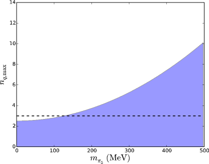
Figure 1: The maximum allowed number of quarks as a function of pion mass to ensure a simulation is in the unbroken phase for the coarse asqtad MILC ensembles ($a\approx 0.125$ fm). The dashed line is $n_{q}=3$ and the shaded region shows allowed values of $n_{q}$ as a function of the pion mass.

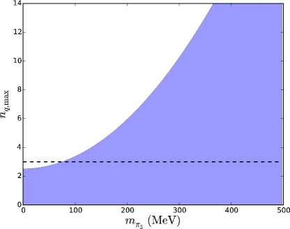
Figure 2: The maximum allowed number of quarks as a function of pion mass to ensure a simulation is in the unbroken phase for the fine asqtad MILC ensembles ($a\approx 0.09$ fm). The dashed line is $n_{q}=3$ and the shaded region shows allowed values of $n_{q}$ as a function of the pion mass.

A simulation is more likely to be in the $A$-phase when we simulate 8 or 12 quarks than when we simulate fewer quarks. More specifically, if the (Goldstone) pion mass is around 500 MeV, the simulation would most likely be in the unbroken phase for 8 quarks (2 flavors, 4 tastes per flavor), while in the $A$-phase for 12 quarks. Figures 1 and 2 were generated using parameters from asqtad MILC ensembles for various lattice spacings. The specific picture will change with different staggered quarks such as nHYP staggered quarks Hasenfratz and Knechtli (2001); Hasenfratz et al. (2007), as are used in Ref. Cheng et al. (2012), but qualitatively we would expect similar results.

In this paper we study the staggered phase diagram for all values of the rS$\chi$PT parameters that may arise during a simulation. In Ref. Aubin and Wang (2004), a third possible phase was discussed (which we will refer to as the $A^{\prime}$-phase) and we show that it cannot occur. Instead, in addition to the $A$-phase, there are two other broken phases that we label the $V$-phase and the $T$-phase. We also show that one of the two broken phases seen in Ref. Cheng et al. (2012) is most likely the $A$-phase discussed in Ref. Aubin and Wang (2004), and suggest other ways to check if indeed this is the case.

We organize this paper as follows. In Sec. II we define the staggered chiral Lagrangian for an arbitrary number of flavors, $n_{f}$, and summarize the results of previous work with the notation we will use in this paper. Then in Sec. III, we find all of the minima of the potential in the revelant region [see Eq. (1)]. We focus on the $A$-phase as that has the features seen in one of the broken phases in Ref. Cheng et al. (2012). Finally we conclude in Sec. IV. We include two appendices where we list the masses in the $A$-phase and the $T$-phase in Appendix A and Appendix B, respectively.

II The Staggered Chiral Lagrangian

The starting point of our analysis is the S$\chi$PT Lagrangian for $n_{f}$ flavors of quarks Aubin and Bernard (2003). The Lagrangian is written in terms of the field $\Sigma=\exp(i\Phi/f)$, a $4n_{f}\times 4n_{f}$ matrix, with

$$\Phi=\left(\begin{array}[]{cccc}U&\pi^{+}&K^{+}&\cdots\\ \pi^{-}&D&K^{0}&\cdots\\ K^{-}&\bar{K^{0}}&S&\cdots\\ \vdots&\vdots&\vdots&\ddots\end{array}\right)\ .$$ (8)

The elements shown are each $4\times 4$ matrices that are linear combinations of the hermitian generators,

$$T_{a}=\{\xi_{5},i\xi_{\mu 5},i\xi_{\mu\nu},\xi_{\mu},\xi_{I}\}.$$ (9)

In euclidean space, the gamma matrices $\xi_{\mu}$ are hermitian, and we use the notations $\xi_{\mu\nu}\equiv\xi_{\mu}\xi_{\nu}$ [$\mu<\nu$ in Eq. (9)], $\xi_{\mu 5}\equiv\xi_{\mu}\xi_{5}$ and $\xi_{I}\equiv I$ is the $4\times 4$ identity matrix. Under the chiral $SU(4n_{f})_{L}\times SU(4n_{f})_{R}$ symmetry, $\Sigma\to L\Sigma R^{\dagger}$. The components of the diagonal (flavor-neutral) elements ($U_{a}$, $D_{a}$, $S_{a}$, etc.) are real, while the off-diagonal (flavor-charged) fields are complex ($\pi^{+}_{a}$, $K^{0}_{a}$, etc.), such that $\Phi$ is hermitian.

From Ref. Aubin and Bernard (2003), the Lagrangian is given by

$$\mathcal{L} = \frac{f^{2}}{8}\operatorname{Tr}(\partial_{\mu}\Sigma\partial_{\mu}\Sigma^{\dagger})-\frac{1}{4}\mu f^{2}\operatorname{Tr}(\mathcal{M}\Sigma+\mathcal{M}\Sigma^{\dagger})$$ (10)

$${}+\frac{2m_{0}^{2}}{3}(U_{I}+D_{I}+S_{I}+\cdots)^{2}+a^{2}\mathcal{V},$$

where $\mu$ is a constant with dimensions of mass, $f$ is the tree-level pion decay constant (normalized here so that $f_{\pi}\approx 131$ MeV), and the $m_{0}^{2}$ term includes the $n_{f}$ flavor-neutral taste-singlet fields. Normally, in physical calculations, we would take $m_{0}\to\infty$ at the end to decouple the taste-singlet $\eta^{\prime}_{I}$, however in a broken phase there is no physical reason to assume a large value for $m_{0}$, so we will retain that parameter in our calculations. Finally, $\mathcal{V}=\mathcal{U}+\mathcal{U}\,^{\prime}$ is the taste-symmetry breaking potential given by

$$-\mathcal{U} = C_{1}\operatorname{Tr}(\xi^{(n_{f})}_{5}\Sigma\xi^{(n_{f})}_{5}\Sigma^{\dagger})$$ (11)

$$+C_{3}\frac{1}{2}\sum_{\nu}[\operatorname{Tr}(\xi^{(n_{f})}_{\nu}\Sigma\xi^{(n_{f})}_{\nu}\Sigma)+h.c.]$$

$$+C_{4}\frac{1}{2}\sum_{\nu}[\operatorname{Tr}(\xi^{(n_{f})}_{\nu 5}\Sigma\xi^{(n_{f})}_{5\nu}\Sigma)+h.c.]$$

$$+C_{6}\ \sum_{\mu<\nu}\operatorname{Tr}(\xi^{(n_{f})}_{\mu\nu}\Sigma\xi^{(n_{f})}_{\nu\mu}\Sigma^{\dagger})\,,$$

$$-\mathcal{U}\,^{\prime} = C_{2V}\frac{1}{4}\sum_{\nu}[\operatorname{Tr}(\xi^{(n_{f})}_{\nu}\Sigma)\operatorname{Tr}(\xi^{(n_{f})}_{\nu}\Sigma)+h.c.]$$ (12)

$$+C_{2A}\frac{1}{4}\sum_{\nu}[\operatorname{Tr}(\xi^{(n_{f})}_{\nu 5}\Sigma)\operatorname{Tr}(\xi^{(n_{f})}_{5\nu}\Sigma)+h.c.]$$

$$+C_{5V}\frac{1}{2}\sum_{\nu}[\operatorname{Tr}(\xi^{(n_{f})}_{\nu}\Sigma)\operatorname{Tr}(\xi^{(n_{f})}_{\nu}\Sigma^{\dagger})]$$

$$+C_{5A}\frac{1}{2}\sum_{\nu}[\operatorname{Tr}(\xi^{(n_{f})}_{\nu 5}\Sigma)\operatorname{Tr}(\xi^{(n_{f})}_{5\nu}\Sigma^{\dagger})]\ .$$

The $\xi^{(n_{f})}_{B}$ in $\mathcal{V}$ are the block-diagonal $4n_{f}\times 4n_{f}$ matrices

$$\xi_{B}^{(n_{f})}=\left(\begin{array}[]{cccc}\xi_{B}&0&0&\cdots\\ 0&\xi_{B}&0&\cdots\\ 0&0&\xi_{B}&\cdots\\ \vdots&\vdots&\vdots&\ddots\end{array}\right),$$ (13)

with $B\in\{5,\mu 5,\mu\nu(\mu<\nu),\mu,I\}$. The mass matrix, $\mathcal{M}$, is the $4n_{f}\times 4n_{f}$ diagonal matrix $\mathcal{M}=mI_{4n_{f}\times 4n_{f}}$, as we are only interested in the degenerate case that is relevant for these BSM studies.

As is well known Lee and Sharpe (1999); Aubin and Bernard (2003), while this potential breaks the taste symmetry at $\mathcal{O}(a^{2})$, an accidental $SO(4)$ symmetry remains. This implies a degeneracy in the masses among different tastes of a given flavor meson, which is seen in the tree-level masses of the pseudoscalar mesons. We can classify these mesons into irreducible representations of $SO(4)$. The mass for the meson $M$ (composed of quarks $a$ and $b$) with taste $B$, is given at tree-level by

$$m^{2}_{M_{B}}=\mu\left(m_{a}+m_{b}\right)+a^{2}\Delta_{B}\ ,$$ (14)

for mesons composed of different quarks, and

$$m^{2}_{M_{B}}=2\mu m_{a}+a^{2}\Delta_{B}+\frac{n_{f}n_{t}}{4}a^{2}\delta^{\prime}_{B-}\ ,\quad B=V,A\ ,$$ (15)

for the flavor-neutral mesons. The $\Delta_{B}$’s are given in Ref. Aubin and Bernard (2003) and are linear combinations of the coefficients in the potential $\mathcal{U}$ and we have the hairpin terms,

$$\delta^{\prime}_{V(A)\pm}\equiv\frac{16}{f^{2}}\left[C_{2V(A)}\pm C_{5V(A)}\right]\ .$$ (16)

The difference in Eq. (15) from previous works is that we have the factor $n_{f}n_{t}/4$ in front of the hairpin parameter. This arises using the replica method Bernard (2006) to write our expressions for general numbers of flavors and tastes. Of course, $n_{f}$ is the number of (degenerate) staggered flavors in our calculation, while $n_{t}$ is the number of tastes per flavor we wish to keep (hence the factor of 1/4). The factor $n_{f}n_{t}\equiv n_{q}$ will be the number of degenerate fermions we have in our theory.

Given that empirically the $\Delta_{B}$’s are all positive in simulations, $\delta^{\prime}_{V-}$ is consistent with zero, and $\delta^{\prime}_{A-}<0$ Aubin et al. (2004); Bazavov et al. (2010); Bernard , focus has been on the possibility of a negative mass-squared arising with the $\eta^{\prime}_{A}$ meson. It was shown in Ref. Aubin and Wang (2004) that in current $2+1$-flavor simulations, it is very unlikely the simulation will be performed in this phase. Instead, there has been evidence of this phase appearing in BSM simulations Cheng et al. (2012), and this can easily be understood from Eq. (14). As discussed in the Introduction, and shown in Figs. 1 and 2, assuming that the actual value of $\delta^{\prime}_{A-}$ is, to a first approximation, dependent only upon the specific fermion formulation and not the number of flavors (or tastes), then as $n_{q}$ increases, the simulations are more likely to be performed in the phase described in Ref. Aubin and Wang (2004).

As discussed in Ref. Aubin and Wang (2004), in the $A$-phase, all of the squared meson masses will be positive given the relationships between the different parameters, except possibly for the tensor taste flavor singlet, $\eta^{\prime}_{ij}$. Specifically, we have (rewriting this expression with our notation),

$$m^{2}_{\eta^{\prime}_{ij}} = -\frac{n_{f}n_{t}}{4}a^{2}\delta_{A-}^{\prime}-\frac{n_{f}n_{t}}{4}a^{2}\delta_{V+}^{\prime}$$ (17)

$${}+\frac{16m^{2}\mu^{2}\left(a^{2}\Delta_{T}-a^{2}\Delta_{A}+\frac{n_{f}n_{t}}{4}a^{2}\delta_{V+}^{\prime}\right)}{\left(a^{2}\Delta_{A}+\frac{n_{f}n_{t}}{4}a^{2}\delta_{A-}^{\prime}\right)^{2}}.$$

The parameter $\delta_{V+}^{\prime}$ in this expression has not yet been measured, and as such, $m^{2}_{\eta^{\prime}_{ij}}$ has the possibility of going negative. This new phase, which we denote the $A^{\prime}$-phase, could in principle arise in the staggered phase diagram. In the next section we study the phase diagram in general and find that this is not the case, while additional phases other than the $A^{\prime}$-phase do exist.

III General phase diagram

To find the vacuum state of the theory, we must minimize the potential,

$$\mathcal{W}=-\frac{1}{4}\mu mf^{2}\operatorname{Tr}(\Sigma+\Sigma^{\dagger})+a^{2}\mathcal{U}+a^{2}\mathcal{U}\,^{\prime}\ ,$$ (18)

where we have already substituted $\mathcal{M}=mI_{4n_{f}\times 4n_{f}}$. This calculation is most simply done in the physical basis, where everything is written in terms of (for three flavors) $\pi^{0}$, $\eta$, and $\eta^{\prime}$ instead of the flavor-basis mesons $U$, $D$, and $S$. For degenerate quarks, we define the singlet as

$$\eta^{\prime}_{B}=\frac{1}{\sqrt{n_{f}}}\left(U_{B}+D_{B}+S_{B}+\cdots\right)\,,$$ (19)

for any number of flavors/tastes. As these are the mesons most likely to acquire a negative mass-squared, we focus solely on these. From here on we remark that in the degenerate quark mass limit, the octet meson masses of a given taste have equal masses which we denote with $m_{\pi}$, while the $\eta^{\prime}$ masses are distinct from these. We note that the number of flavors $n_{f}$ (so long as it’s greater than 1) will not affect our results; $n_{f}$ will only indicate a greater likelihood of being in the broken phase at this point.

Generally, $\delta^{\prime}_{A-}$ and $\delta^{\prime}_{V-}$ are the parameters likely to be negative, and they only arise in the $\eta^{\prime}$ masses. We infer the symmetry breaking to only occur in the $\eta^{\prime}$ direction in flavor space. Therefore, we are going to keep only this meson in our expression for $\Phi$ when looking for the minima of the potential in Eq. (18). This will be valid right near the critical point, and since we are looking at this perturbatively, we are looking only at small fluctuations about the minimum. So long as no other squared mass goes negative in the phase, our results should give us the correct mass spectrum for the broken phase. If a squared mass does go negative, as in Eq. (17) for certain values of $\delta^{\prime}_{V+}$, we are not near a minimum of the potential, and thus such additional phases are not stable.

Keeping only the $\eta^{\prime}_{B}$, $\Phi$ and $\Sigma$ are block-diagonal in flavor space. We can write the condensate $\langle\Sigma\rangle$ in terms of the 16 real numbers $\sigma_{I},\sigma_{\mu 5},\sigma_{\mu\nu}(\mu<\nu),\sigma_{\mu},$ and $\sigma_{5}$,

$$\langle\Sigma\rangle=\sigma_{I}\left(I_{4n_{f}\times 4n_{f}}\right)+i\sigma_{\mu 5}\left(i\xi^{(n_{f})}_{\mu 5}\right)+i\sigma_{\mu\nu}\left(i\xi^{(n_{f})}_{\mu\nu}\right)+i\sigma_{\mu}\xi^{(n_{f})}_{\mu}+i\sigma_{5}\left(i\xi^{(n_{f})}_{5}\right)\ ,$$ (20)

with the condition that $\sum_{B}\sigma_{B}^{2}=1$. Upon substituting this into the potential, we find the potential (not surprisingly) is only dependent upon the magnitudes of these sets of coefficients, given by

$$\sigma_{A} = \left(\sum_{\mu}\sigma_{\mu 5}^{2}\right)^{1/2}\ ,$$ (21)

$$\sigma_{T} = \left(\sum_{\mu<\nu}\sigma_{\mu\nu}^{2}\right)^{1/2}\ ,$$ (22)

$$\sigma_{V} = \left(\sum_{\mu}\sigma_{\mu}^{2}\right)^{1/2}\ ,$$ (23)

so that we have, up to an unimportant constant and for arbitrary numbers of flavors/tastes,

$$\mathcal{W} = -\frac{3f^{2}}{2}\biggl{[}4\mu m\sigma_{I}-\sigma_{A}^{2}\left(a^{2}\Delta_{A}+\frac{n_{f}n_{t}}{4}a^{2}\delta^{\prime}_{A-}\right)$$ (24)

$${}-\sigma_{V}^{2}\left(a^{2}\Delta_{V}+\frac{n_{f}n_{t}}{4}a^{2}\delta^{\prime}_{V-}\right)-\sigma_{T}^{2}a^{2}\Delta_{T}\biggr{]}\ .$$

When minimizing this potential we find three distinct non-trivial phases:

$$A\textrm{-phase} : a^{2}\Delta_{A}+\frac{n_{f}n_{t}}{4}a^{2}\delta^{\prime}_{A-}<-2\mu m\ ,$$ (25)

$$V\textrm{-phase} : a^{2}\Delta_{V}+\frac{n_{f}n_{t}}{4}a^{2}\delta^{\prime}_{V-}<-2\mu m\ ,$$ (26)

$$T\textrm{-phase} : a^{2}\Delta_{T}<-2\mu m\ .$$ (27)

The $A$-phase was discussed in detail in Ref. Aubin and Wang (2004), and the results for the $V$-phase are identical to those for the $A$-phase with the replacement $A\leftrightarrow V$ in all of the relevant equations. The $T$-phase is distinct here, and it is unlikely that a simulation will be performed in this phase. This is because all of the parameters $\Delta_{B}$ are positive in simulations, so these conditions are only likely to hold for the $A$ and $V$ phases because the parameters $\delta^{\prime}_{A-}$ and $\delta^{\prime}_{V-}$ tend to be negative. Nevertheless, we discuss this phase briefly in the Appendix for completeness. We note that in principle, more than one of the conditions in Eqs. (25) through (27) may hold simultaneously, but in fact we only see these three phases. This implies that only one condition will point to the true minimum about which to expand. In the unlikely case that two of the left-hand sides are equal, for example,

$$a^{2}\Delta_{T}=a^{2}\Delta_{A}+\frac{n_{f}n_{t}}{4}a^{2}\delta^{\prime}_{A-}\ ,$$ (28)

this would introduce a symmetry between (in this case) the axial- and tensor-tastes, but this does not introduce a distinct phase.

We note that none of these three broken phases correspond to the $A^{\prime}$-phase discussed in the previous section. Approaching this phase from $A$-phase, we find a saddle point in the potential, and as such this is an unstable equilibrium point. Thus, we will not explore that case further.

We have for the $A$-phase,

$$\sigma_{T}=\sigma_{V}=0,\ \sigma_{I}\equiv\cos\theta_{A}=\frac{-2\mu m}{a^{2}\Delta_{A}+\frac{n_{f}n_{t}}{4}a^{2}\delta^{\prime}_{A-}},\ \sigma_{A}=\sqrt{1-\sigma_{I}^{2}}\ ,$$ (29)

the $V$-phase,

$$\sigma_{T}=\sigma_{A}=0,\ \sigma_{I}\equiv\cos\theta_{V}=\frac{-2\mu m}{a^{2}\Delta_{V}+\frac{n_{f}n_{t}}{4}a^{2}\delta^{\prime}_{V-}},\ \sigma_{V}=\sqrt{1-\sigma_{I}^{2}}\ ,$$ (30)

and for the $T$-phase,

$$\sigma_{A}=\sigma_{V}=0,\ \sigma_{I}\equiv\cos\theta_{T}=\frac{-2\mu m}{a^{2}\Delta_{T}},\ \sigma_{T}=\sqrt{1-\sigma_{I}^{2}}\ .$$ (31)

These break the remnant $SO(4)$ symmetry [to $SO(3)$ for the $A$ and $V$ phases, and to $SO(2)\times SO(2)$ for the $T$ phase]. The direction of each of the vectors $a_{\mu},$ $a_{\mu 5}$, and $a_{\mu\nu}$ is arbitrary, and we will choose a particular direction in Eqs. (32) and (33).

In each of these cases, we have the condensate of the form

$$\left\langle\Sigma\right\rangle = \left(\begin{matrix}\exp\left[i\theta_{B}T_{B}\right]&0&0&\cdots\\ 0&\exp\left[i\theta_{B}T_{B}\right]&0&\cdots\\ 0&0&\exp\left[i\theta_{B}T_{B}\right]&\cdots\\ \vdots&\vdots&\vdots&\ddots\end{matrix}\right)\,,$$ (32)

where $B=A,V,T$, and

$$T_{B}=\begin{cases}i\xi_{45}&A-{\rm phase}\\ \xi_{4}&V-{\rm phase}\\ i\xi_{12}&T-{\rm phase}\end{cases}\ .$$ (33)

In each of these cases, the shift-symmetry Lee and Sharpe (1999); Aubin and Bernard (2003); Aubin and Wang (2004) that exists which has the form in the chiral theory,

$$\Sigma\to\xi^{(n_{f})}_{\mu}\Sigma\xi^{(n_{f})}_{\mu}\ ,$$ (34)

is broken. Thus, as was seen in Ref. Cheng et al. (2012), one can use the difference between neighboring plaquettes and the difference between neighboring links to determine if we are in a broken phase. However, those parameters are sensitive only to the breaking of the single-site shift symmetry, so they cannot distinguish between the $A$, $V$, or $T$-phase. Thus, for a complete understanding of the phase seen in the simulation, the mass spectrum should also be studied.

The key difference between the unbroken phase and the various broken phases is that the squared-meson masses in the broken phases have the generic form

$$m^{2}_{M}=\mathcal{A}+\mathcal{B}m^{2}\ .$$ (35)

Here $\mathcal{A}$ and $\mathcal{B}$ are independent of the quark mass but are dependent upon $a$. Unlike the unbroken phase, the squared meson masses are linear in $m^{2}$ as opposed to $m$, and for some mesons $\mathcal{B}=0$ so that the mesons have a mass independent of the quark mass.

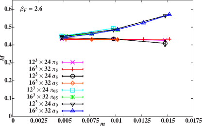
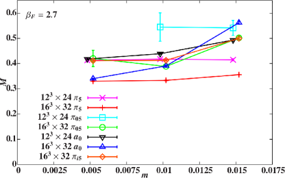
(a)                                                                    (b)

Figure 3: Figure 7 from Ref. Cheng et al. (2012), showing the masses of the $\pi_{5}$ and $\pi_{05}$ ($\pi_{45}$ in our notation) as a function of the quark mass. (a) shows the masses in the broken phase discussed here and (b0 shows the masses in the unbroken phase.

Figure 3 is a reprint of Fig. 7 from Ref. Cheng et al. (2012), which shows the masses for the pseudoscalar taste pion as well as the taste-45 pion for two lattice spacings. Fig. 3(a) shows one of the two broken phases seen as a function of the input quark mass for 12 quarks (in our notation we would set $n_{f}=3,n_{t}=4$). Of the two phase transitions discussed in that paper, the chiral effective theory seems useful for understanding the second here (that appears at smaller lattice spacing around $\beta\approx 2.7$ in Ref. Cheng et al. (2012)). The authors of Ref. Cheng et al. (2012) show that the single-site shift symmetry is broken in this phase, and we now argue that this is likely the $A$-phase.

The $\pi_{5}$ in Fig. 3(a) has an approximately constant mass as a function of the quark mass, which would be consistent with the calculation of Ref. Aubin and Wang (2004):

$$m^{2}_{\pi_{5}}=-\frac{n_{f}n_{t}}{4}a^{2}\delta^{\prime}_{A-}\ ,$$ (36)

(recall $\delta^{\prime}_{A-}<0$ in this phase), and the taste-45 mass has the form,

$$m^{2}_{\pi_{45}}=m^{2}_{\pi_{5}}+a^{2}\Delta_{A}\bar{\mu}^{2}m^{2}\ ,$$ (37)

where $\bar{\mu}$ is defined below in Eq. (38). Were this the $V$-phase, the $\pi_{5}$ would still have a constant mass, but the $\pi_{4}$ would have the behavior of Eq. (37) (with $\Delta_{A}\to\Delta_{V}$). Similarly, were this the $T$-phase, as can be seen in Appendix B, the $\pi_{5}$ mass is dependent upon the quark mass while the $\pi_{45}$ mass is constant.

We can see that as $m\to 0$, $m_{\pi_{45}}\to m_{\pi_{5}}$ as rS$\chi$PT predicts. This gives credence to the fact that the intermediate phase seen in Ref. Cheng et al. (2012) is in fact this $A$-phase, but a more detailed analysis would require several things. First, one should perform a fit to the forms above for the taste-45 and taste-5 pions. More importantly, one should measure of all of the different taste meson masses to see the pattern as predicted in Ref. Aubin and Wang (2004) (and shown in Appendix A). Figure 3(b) shows the other side of the transition (larger $\beta$, and thus a smaller lattice spacing), and immediately shows a different pattern: The four axial-taste pions are nearly degenerate and the difference $m_{\pi_{\mu 5}}^{2}-m_{\pi_{5}}^{2}\approx$ constant as a function of $m$. This is (roughly) the pattern seen in the physical regime of rS$\chi$PT Lee and Sharpe (1999); Aubin and Bernard (2003).

We show in Figs. 4 and 5 plots of $m_{\pi}$ vs. $m$ and $m_{\eta}$ vs. $m$ for the different tastes in the $A$-phase. The units in these plots are arbitrary, chosen so that the values $m>2$ correspond to the unbroken phase. The solid red lines in Fig. 4 correspond to the $\pi_{5}$ and $\pi_{45}$ masses, which are to be compared with the masses shown in the left-hand plot of Fig. 7 in Ref. Cheng et al. (2012).

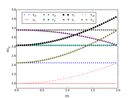
Figure 4: $m_{\pi}$ vs. the quark mass in the $A$-phase in arbitrary units. These units are such that when $m\geq 2$ the system is in the unbroken phase again. The solid line corresponds to $m_{\pi_{5}}$ and the dashed line to $m_{\pi_{45}}$.

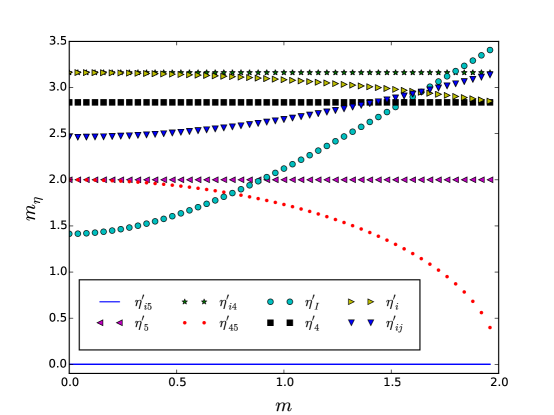
Figure 5: $m_{\eta}$ vs. the quark mass in the $A$-phase in arbitrary units. These units are such that when $m\geq 2$ the system is in the unbroken phase again. The solid line at $m_{\eta}=0$ corresponds to the three Goldstone bosons in this phase.

As for the phase at stronger coupling, it is unlikely that rS$\chi$PT could explain this region. As we have seen in this work, rS$\chi$PT shows that there should be at most four phases: the unbroken phase as well as the $A$, $T$, and $V$ phases. However, these all are within the regime governed by the constraint in Eq. (1), most importantly that $a^{2}\Lambda^{2}_{\rm QCD}\ll 1$. The stronger coupling phase likely violates this constraint, and thus the chiral theory is not valid in this regime. Nevertheless, it would be instructive to understand more about the intermediate phase to be sure that rS$\chi$PT is in fact describing the region as we expect it is.

IV Conclusion

We have studied the complete phase diagram for staggered quarks with an arbitrary number of degenerate flavors, at least within the window given in Eq. (1). In this regime, there are only four phases: one unbroken (physical) phase, as well as three phases where the (approximate) $\mathcal{O}(a^{2})$ accidental $SO(4)$ symmetry is broken. Of these three phases, as seen previously Aubin and Wang (2004), only one phase (the $A$-phase) is likely to be seen in simulations, but only if one looks at theories with 8 or 12 flavors of quarks Cheng et al. (2012). The additional possible phase that was suggested to exist in Ref. Aubin and Wang (2004) [when the squared mass of the $\eta^{\prime}_{ij}$, Eq. (17), goes negative] does not correspond to a stable region.

While rS$\chi$PT cannot fully explain both broken phases seen in Ref. Cheng et al. (2012), it can give a picture of broken phases that are located close to the unbroken phase (as a function of the lattice spacing). Studying the plaquette & link differences as well as as the staggered meson mass spectrum would allow one to determine specifically which region of the phase diagram the simulation is in. For BSM studies this is essential as it is more likely to enter these unphysical regimes for additional quark flavors.

Appendix A $A$-Phase

In this appendix we list the meson masses that appear in the $A$-phase Aubin and Wang (2004). Here we put them in terms of $n_{f}n_{t}$ as above, and we define

$$\overline{\mu}\equiv\frac{-2\mu}{a^{2}\Delta_{A}+\frac{n_{f}n_{t}}{4}a^{2}\delta^{\prime}_{A-}}\ .$$ (38)

The first masses we list are constant in the quark mass:

$$m^{2}_{\eta^{\prime}_{i5}} = 0\ ,$$ (39)

$$m^{2}_{\eta^{\prime}_{5}}=m^{2}_{\pi_{5}} = -a^{2}\Delta_{A}-\frac{n_{f}n_{t}}{4}a^{2}\delta^{\prime}_{A-}\ ,$$ (40)

$$m^{2}_{\pi_{i5}} = -\frac{n_{f}n_{t}}{4}a^{2}\delta^{\prime}_{A-}\ ,$$ (41)

$$m^{2}_{\pi_{i4}}=m^{2}_{\eta^{\prime}_{i4}} = m^{2}_{\pi_{5}}+a^{2}\Delta_{T}\ ,$$ (42)

$$m^{2}_{\eta^{\prime}_{4}} = m^{2}_{\pi_{5}}+a^{2}\Delta_{V}+\frac{n_{f}n_{t}}{4}a^{2}\delta^{\prime}_{V-}\ ,$$ (43)

$$m^{2}_{\pi_{4}} = m^{2}_{\pi_{5}}+a^{2}\Delta_{V}\ .$$ (44)

We note that Eq. (26) in Ref. Aubin and Wang (2004) [corresponding to our Eq. (43)] has a typo, as the final term in that expression should be $+\frac{3}{4}a^{2}\delta^{\prime}_{V}$ in that paper’s notation, not $-\frac{3}{4}a^{2}\delta^{\prime}_{V}$. With the above, we can determine the constants,

$$\Delta_{A},\quad\delta^{\prime}_{A-},\quad\Delta_{T},\quad\Delta_{V},\quad\delta^{\prime}_{V-}\ .$$

Then

$$m^{2}_{\pi_{45}} = m^{2}_{\pi_{5}}+a^{2}\Delta_{A}\bar{\mu}^{2}m^{2}$$ (45)

allows us to determine $\bar{\mu}$. With

$$m^{2}_{\pi_{I}} = m^{2}_{\pi_{5}}+\bar{\mu}^{2}m^{2}\left(a^{2}\Delta_{I}-a^{2}\Delta_{V}\right)+a^{2}\Delta_{V}$$ (46)

$$m^{2}_{\eta^{\prime}_{I}} = n_{t}m_{0}^{2}+m^{2}_{\pi_{5}}-\frac{n_{f}n_{t}}{4}a^{2}\delta^{\prime}_{A+}+a^{2}\Delta_{V}$$ (47)

$${}+\bar{\mu}^{2}m^{2}\biggl{(}\frac{n_{f}n_{t}}{4}a^{2}\delta^{\prime}_{A+}+a^{2}\Delta_{I}-a^{2}\Delta_{V}\biggr{)}$$

allows us to determine $\Delta_{I}$ and $\delta^{\prime}_{A+}$ respectively, and finally

$$m_{\eta^{\prime}_{ij}}^{2} = \bar{\mu}^{2}m^{2}m^{2}_{\pi_{i4}}-\frac{n_{f}n_{t}}{4}\left(1-\bar{\mu}^{2}m^{2}\right)(a^{2}\delta^{\prime}_{A-}+a^{2}\delta^{\prime}_{V+})$$ (48)

for $\delta^{\prime}_{V+}$.

The following four masses are then determined from those above results,

$$m^{2}_{\pi_{i}} = m^{2}_{\pi_{5}}+(m^{2}_{\pi_{4}}-m^{2}_{\pi_{5}})\bar{\mu}^{2}m^{2}+(m^{2}_{\eta^{\prime}_{i4}}-m^{2}_{\pi_{5}})(1-\bar{\mu}^{2}m^{2})\ ,$$ (49)

$$m^{2}_{\pi_{ij}} = m^{2}_{\pi_{i5}}+\bar{\mu}^{2}m^{2}\left(m^{2}_{\eta^{\prime}_{i4}}-m^{2}_{\pi_{i5}}\right)\ ,$$ (50)

$$m^{2}_{\eta^{\prime}_{45}} = m^{2}_{\pi_{5}}\left(1-\bar{\mu}^{2}m^{2}\right)\ ,$$ (51)

$$m^{2}_{\eta^{\prime}_{i}} = m^{2}_{\eta^{\prime}_{i4}}-(m^{2}_{\eta^{\prime}_{i4}}-m^{2}_{\eta^{\prime}_{4}})\bar{\mu}^{2}m^{2}\ .$$ (52)

This shows that we have non-trivial relationships between the various masses. Additionally, as seen in Figs. 4 and 5 we have several crossings of the meson masses for both the $\pi$ and the $\eta$. While those figures are for a specific set of parameters, they are indicative of the qualitative features of the $A$-phase.

Appendix B $T$-Phase

In this appendix we list the masses for the mesons in the $T$-phase, where just as before, the octet masses are equal. In this case we define

$$\bar{\mu}\equiv\frac{2\mu}{-a^{2}\Delta_{T}}\ .$$ (53)

Thus we have

$$m^{2}_{\pi_{5}}=m^{2}_{\eta^{\prime}_{5}} = -a^{2}\Delta_{T}\bar{\mu}^{2}m^{2}$$ (54)

$$m^{2}_{\pi_{I}} = \bar{\mu}^{2}m^{2}\left(a^{2}\Delta_{I}-a^{2}\Delta_{T}\right)$$ (55)

$$m^{2}_{\eta^{\prime}_{I}} = n_{t}m_{0}^{2}+\bar{\mu}^{2}m^{2}\left(a^{2}\Delta_{I}-a^{2}\Delta_{T}\right)$$ (56)

$$m^{2}_{\pi_{12}}=m^{2}_{\eta^{\prime}_{12}} = -a^{2}\Delta_{T}(1-\bar{\mu}^{2}m^{2})$$ (57)

$$m^{2}_{\pi_{34}}=m^{2}_{\eta^{\prime}_{34}} = \left(a^{2}\Delta_{I}-a^{2}\Delta_{T}\right)(1-\bar{\mu}^{2}m^{2})$$ (58)

$$m^{2}_{\eta^{\prime}_{1}}=m^{2}_{\eta^{\prime}_{2}} = a^{2}\Delta_{V}-a^{2}\Delta_{T}+\frac{n_{f}n_{t}}{4}a^{2}\delta^{\prime}_{V-}$$ (59)

$$m^{2}_{\eta^{\prime}_{3}}=m^{2}_{\eta^{\prime}_{4}} = a^{2}\Delta_{V}-a^{2}\Delta_{T}-\frac{n_{f}n_{t}}{4}(1-\bar{\mu}^{2}m^{2})a^{2}\delta^{\prime}_{A+}$$ (60)

$${}+\frac{n_{f}n_{t}}{4}\bar{\mu}^{2}m^{2}a^{2}\delta^{\prime}_{V-}$$

$$m^{2}_{\eta^{\prime}_{15}}=m^{2}_{\eta^{\prime}_{25}} = a^{2}\Delta_{A}-a^{2}\Delta_{T}+\frac{n_{f}n_{t}}{4}a^{2}\delta^{\prime}_{A-}$$ (61)

$$m^{2}_{\eta^{\prime}_{35}}=m^{2}_{\eta^{\prime}_{45}} = a^{2}\Delta_{A}-a^{2}\Delta_{T}-\frac{n_{f}n_{t}}{4}a^{2}\delta^{\prime}_{V+}$$ (62)

$${}+\frac{n_{f}n_{t}}{4}\bar{\mu}^{2}m^{2}\left(a^{2}\delta^{\prime}_{A-}+a^{2}\delta^{\prime}_{V+}\right)$$

$$m^{2}_{\pi_{\mu 5}} = a^{2}\Delta_{A}-a^{2}\Delta_{T}$$ (63)

$$m^{2}_{\pi_{\mu}} = a^{2}\Delta_{V}-a^{2}\Delta_{T}$$ (64)

$$m^{2}_{\eta^{\prime}_{24}}=m^{2}_{\eta^{\prime}_{23}}=m^{2}_{\eta^{\prime}_{14}}=m^{2}_{\eta^{\prime}_{13}} = 0$$ (65)

$$m^{2}_{\pi_{24}}=m^{2}_{\pi_{23}}=m^{2}_{\pi_{14}}=m^{2}_{\pi_{13}} = 0$$ (66)

With $\Delta_{T}$ “large and negative,” these are all positive or zero with the exception of those with the $\delta^{\prime}_{A+}$ or $\delta^{\prime}_{V+}$ terms. As in the $A$ or $V$ phase, if those parameters are such that $m^{2}_{\eta^{\prime}_{45}}<0$ (for example), this leads to a phase that would not give rise to a stable ground state.

The generic dependence $m_{\pi}^{2}=\mathcal{A}+\mathcal{B}m^{2}$ persists in this phase, but for one we see a different pattern than in the $A$ or $V$ phases. Additionally, there are no mixings between different taste mesons. Nevertheless, it is unlikely, given the empirical evidence, that one would be able to run a simulation in this phase, and as such we will not discuss this phase further.

ACKNOWLEDGMENTS

We would like to thank Claude Bernard, Anna Hasenfratz, and Steve Sharpe for useful discussions. Additionally we would like to thank Claude Bernard for helpful comments on the manuscript.

References

- Aoki (1984) S. Aoki, Phys. Rev. D30, 2653 (1984).
- Sharpe and Singleton (1998) S. R. Sharpe and R. L. Singleton, Jr, Phys. Rev. D58, 074501 (1998), eprint hep-lat/9804028.
- Lee and Sharpe (1999) W.-J. Lee and S. R. Sharpe, Phys. Rev. D60, 114503 (1999), eprint hep-lat/9905023.
- Aubin and Bernard (2003) C. Aubin and C. Bernard, Phys. Rev. D68, 034014 (2003), eprint hep-lat/0304014.
- Aubin and Wang (2004) C. Aubin and Q.-h. Wang, Phys. Rev. D70, 114504 (2004), eprint hep-lat/0410020.
- Aubin et al. (2004) C. Aubin, C. Bernard, C. E. DeTar, J. Osborn, S. Gottlieb, E. B. Gregory, D. Toussaint, U. M. Heller, J. E. Hetrick, and R. Sugar (MILC), Phys. Rev. D70, 114501 (2004), eprint hep-lat/0407028.
- Bazavov et al. (2010) A. Bazavov et al. (MILC), Rev. Mod. Phys. 82, 1349 (2010), eprint 0903.3598.
- Cheng et al. (2012) A. Cheng, A. Hasenfratz, and D. Schaich, Phys. Rev. D85, 094509 (2012), eprint 1111.2317.
- Bernard (2006) C. Bernard, Phys. Rev. D73, 114503 (2006), eprint hep-lat/0603011.
- (10) C. Bernard, private communication.
- Hasenfratz and Knechtli (2001) A. Hasenfratz and F. Knechtli, Phys. Rev. D64, 034504 (2001), eprint hep-lat/0103029.
- Hasenfratz et al. (2007) A. Hasenfratz, R. Hoffmann, and S. Schaefer, JHEP 05, 029 (2007), eprint hep-lat/0702028.