MERLiN: Mixture Effect Recovery in Linear Networks

Abstract

Causal inference concerns the identification of cause-effect relationships between variables, e. g. establishing whether a stimulus affects activity in a certain brain region. The observed variables themselves often do not constitute meaningful causal variables, however, and linear combinations need to be considered. In electroencephalographic studies, for example, one is not interested in establishing cause-effect relationships between electrode signals (the observed variables), but rather between cortical signals (the causal variables) which can be recovered as linear combinations of electrode signals.

We introduce MERLiN (Mixture Effect Recovery in Linear Networks), a family of causal inference algorithms that implement a novel means of constructing causal variables from non-causal variables. We demonstrate through application to EEG data how the basic MERLiN algorithm can be extended for application to different (neuroimaging) data modalities. Given an observed linear mixture, the algorithms can recover a causal variable that is a linear effect of another given variable. That is, MERLiN allows us to recover a cortical signal that is affected by activity in a certain brain region, while not being a direct effect of the stimulus. The Python/Matlab implementation for all presented algorithms is available on https://github.com/sweichwald/MERLiN.

I Introduction

Causal inference requires causal variables. Observed variables do not themselves always constitute the causal relata that admit meaningful causal statements, however, and transformations of the variables might be required to isolate causal signals. Images, for example, consist of microscopic variables (pixel colour values) while the identification of meaningful cause-effect relationships requires the construction of macroscopic causal variables (e. g. whether the image shows a magic wand) [1]. That is, it is implausible that a description of effects of changing the colour value of one single pixel, the microscopic variable, leads to characterisation of a meaningful cause-effect relationship; however, the existence of a magic wand, the macroscopic variable, may lead to meaningful statements of the form “manipulating the image such that it shows a magic wand affects the chances of little Maggie favouring this image”. A similar problem often occurs whenever only a linear mixture of causal variables can be observed. In electroencephalography (EEG) studies, for example, measurements at electrodes placed on the scalp are considered to be instantaneously and linearly superimposed electromagnetic activity of sources in the brain [2]. Again, statements about the microscopic variables are meaningless, e. g. “manipulating the electrode’s signal affects the subject’s attentional state”; however, macroscopic variables such as the activity in the parietal cortex, extracted as a linear combination of electrode signals, admit meaningful causal statements such as “manipulating the activity in the parietal cortex affects the subject’s attentional state”. Standard causal inference methods require that all underlying causal variables, i. e., the sources in the brain, are first constructed –or rather recovered– from the observed mixture, i. e., the electrode signals.

There exist a plethora of methods to construct macroscopic variables both from images and linear mixtures. However, prevailing methods to learn visual features [3, 4, 5] ignore the causal aspect, and are fundamentally different from the recent and (to our knowledge) only work that demonstrates how visual causal features can be learned by a sequence of interventional experiments [1]. Likewise, methods to (re-)construct variables from linear mixtures commonly ignore the causal aspect and often rest on implausible assumptions. For instance, independent component analysis (ICA), commonly employed in the analysis of EEG data, rests on the assumption of mutually independent sources [6, 7, 8]. One may argue that muscular or ocular artefacts are independent of the cortical sources and can be extracted via ICA [9, 10]. It seems implausible, though, that cortical sources are mutually independent. In fact, if they were mutually independent there would be no cause-effect relationships between them. Thus, methods ignoring the causal aspect are unsuited to construct meaningful causal variables.

Mixture Effect Recovery in Linear Networks (MERLiN) aims to construct a causal variable from a linear mixture without requiring multiple interventional experiments. The fundamental idea is to directly search for statistical in- and dependences that imply, under assumptions discussed below, a certain cause-effect relationship. In essence, given iid samples of a univariate randomised variable $S$, a univariate causal effect $C_{1}$ of $S$, and a multivariate variable $F$, MERLiN searches for a linear combination $\bm{w}$ such that $\bm{w}^{\top}F$ is a causal effect of $C_{1}$, i. e., $S\to C_{1}\to\bm{w}^{\top}F$. This implements the novel idea to construct causal variables such that the resulting statistical properties guarantee meaningful cause-effect relationships.

Figure 1: Problem illustration where $S\to C_{1}\to C_{2}\quad C_{3}$ is the underlying causal graph and $F_{1},F_{2},F_{3}$ are observed variables that are a linear mixture of $C_{1},C_{2},C_{3}$.

As an illustration, consider the directed acyclic graph (DAG) $S\to C_{1}\to C_{2}\quad C_{3}$ shown in Figure 1, where the gap indicates that $C_{3}$ is disconnected from all other variables. In this notation edges denote cause-effect relationships starting at the cause and pointing towards the effect. $S$ denotes a randomised variable. We assume that only a linear mixture $F=\bm{A}[C_{1},C_{2},C_{3}]^{\top}$ ($\bm{A}$ is an unknown mixing matrix) of the causal variables $C_{1},C_{2},C_{3}$ can be observed, and that $\bm{v}$ such that $C_{1}=\bm{v}^{\top}F$ is known. MERLiN’s goal is to recover from the observed linear mixture $F=[F_{1},F_{2},F_{3}]^{\top}$ a causal variable that is an effect of $C_{1}$, i. e., to find $\bm{w}$ such that $\bm{w}^{\top}F$ is an effect of $C_{1}$, where $\bm{w}^{\top}F=C_{2}$ is a valid solution.

We introduce the basic MERLiN${}_{\Sigma^{-1}}$ algorithm that can recover the sought-after causal variable when the cause-effect relationships are linear with additive Gaussian noise (cf. Section III). We also demonstrate how the algorithm can be extended for application to different (neuroimaging) data modalities by (a) including data specific preprocessing steps into the optimisation procedure, and (b) incorporating a priori domain knowledge (cf. Section V). Here, both concepts are demonstrated through application to EEG data when cause-effect relationships within individual frequency bands are of interest.

Thus, we present three related algorithms MERLiN${}_{\Sigma}^{-1}$, MERLiN${}_{\Sigma^{-1}}^{bp}$, and MERLiN${}_{\Sigma^{-1}}^{bp+}$ that are based on optimisation of precision matrix entries (indicated by the subscript $\Sigma^{-1}$). The MERLiN${}_{\Sigma^{-1}}^{bp}$ and MERLiN${}_{\Sigma^{-1}}^{bp+}$ algorithms include preprocessing steps that allow application to timeseries data, identifying a linear combination of timeseries signals such that the resulting log-bandpower (indicated by the superscript $bp$) reveals the sough-after cause-effect relationship. A further extension (indicated by the superscript $bp+$) takes domain knowledge about time-lags into account.

For stimulus-based neuroimaging studies [11], the MERLiN${}_{\Sigma^{-1}}^{bp}$ and MERLiN${}_{\Sigma^{-1}}^{bp+}$ algorithms can establish a cause-effect relationship between brain state features that are observed only as part of a linear mixture. As such, MERLiN is able to provide insights into brain networks beyond those readily obtained from encoding and decoding models trained on pre-defined variables [12]. Furthermore, it employs the framework of Causal Bayesian Networks (CBNs) that has recently been fruitful in the neuroimaging community [13, 14, 15, 16, 12, 17] — the important advantage over methods based on information flow being that it yields testable predictions on the impact of interventions [18, 19].

MERLiN shows good performance both on synthetic and EEG data recorded during neurofeedback experiments. The Python/Matlab implementation for all presented algorithms is available on https://github.com/sweichwald/MERLiN.

II Preliminaries

II-A Causal Bayesian Networks

In general causal inference requires three steps.

1. construction of (causal) variables

2. inference of cause-effect relationships among the variables defined in 1)

3. estimation of the functional form and strength of the causal links established in 2)

In this manuscript we focus on and merge the first two steps. More specifically, a causal variable is implicitly constructed by optimising for properties that at the same time establish a specific cause-effect relationship for this variable. Here we briefly introduce the main aspects of Causal Bayesian Networks (CBNs) that define causation in terms of effects of interventions and allow inference of cause-effect relationships (step 2) from conditional independences in the observed distribution. For an exhaustive treatment see [20, 21].

Definition 1 (Structural Equation Model).

We define a structural equation model (SEM) $\mathcal{{S}}$ as a set of structural equations $X_{i}=f_{i}(\mathbf{{PA}}_{i},N_{i}),\ i\in\mathbb{{N}}_{1:s}\triangleq\{n\in\mathbb{N}:1\leq n\leq s\}$ where the so-called noise variables are independently distributed according to $\mathbb{{P}}_{N_{1},...,N_{s}}=\mathbb{{P}}_{N_{1}}\cdots\mathbb{{P}}_{N_{s}}$. For $i\in\mathbb{{N}}_{1:s}$ the set $\mathbf{{PA}}_{i}\subseteq\{X_{1},...,X_{s}\}\setminus X_{i}$ contains the so-called parents of $X_{i}$ and $f_{i}$ describes how $X_{i}$ relates to the random variables in $\mathbf{{PA}}_{i}$ and $N_{i}$. This induces the unique joint distribution denoted by $\mathbb{{P}}_{\mathcal{{S}}}\triangleq\mathbb{{P}}_{X_{1},...,X_{s}}$.

Replacing at least one of the functions $f_{i},\ i\in\mathbb{{N}}_{1:s}$ by a constant $\spadesuit$ yields a new SEM. We say $X_{i}$ has been intervened on, which is denoted by $\operatorname{do}(X_{i}=\spadesuit)$, leads to the SEM $\mathcal{{S}}|\operatorname{do}(X_{i}=\spadesuit)$, and induces the interventional distribution $\mathbb{{P}}_{\mathcal{{S}}|\operatorname{do}(X_{i}=\spadesuit)}\triangleq\mathbb{{P}}_{X_{1},...,X_{s}|\operatorname{do}(X_{i}=\spadesuit)}$.

Definition 2 (Cause and Effect).

$X_{i}$ is a cause of $X_{j}$ ($i,j\in\mathbb{{N}}_{1:s},\ i\neq j$) wrt. a SEM $\mathcal{{S}}$ iff there exists $\heartsuit\in\mathbb{{R}}$ such that $\mathbb{{P}}_{X_{j}|\operatorname{do}(X_{i}=\heartsuit)}\neq\mathbb{{P}}_{X_{j}}$. $X_{j}$ is an effect of $X_{i}$ iff $X_{i}$ is a cause of $X_{j}$. Often the considered SEM $\mathcal{{S}}$ is omitted if it is clear from the context.

For each SEM $\mathcal{{S}}$ there is a corresponding graph $\mathcal{{G_{S}}}(V,E)$ with $V\triangleq\{X_{1},...,X_{s}\}$ and $E\triangleq\{(X_{i},X_{j}):\ X_{i}\in\mathbf{{PA}}_{j},\ X_{j}\in V\}$ that has the random variables as nodes and directed edges pointing from parents to children. We employ the common assumption that this graph is acyclic, i. e., $\mathcal{{G_{S}}}$ will always be a directed acyclic graph (DAG).

It is insightful to consider the following implication of Definition 2: If in $\mathcal{{G_{S}}}$ there is no directed path from $X_{i}$ to $X_{j}$, $X_{i}$ is not a cause of $X_{j}$ (wrt. $\mathcal{{S}}$). The following example shows that without further assumptions the converse is not true in general, i. e., existence of a path does not generally imply a cause-effect relationship. This nuisance will be accounted for by the faithfulness assumption (cf. Definition 6 below). We provide supportive graphical depictions in Figure 2.

Example 3.

Consider a SEM $S$ with structural equations and graph $\mathcal{{G_{S}}}$ shown in Figure 2a and noise variables $(N_{1},N_{2},N_{3})\sim\mathcal{{N}}(0,1)^{3}$. In $\mathcal{{G_{S}}}$ there is a directed path (in fact even a directed edge) from $X_{1}$ to $X_{3}$ while $\mathbb{{P}}_{X_{3}|\operatorname{do}(X_{1}=\heartsuit)}=\mathbb{{P}}_{X_{3}}=\mathbb{{P}}_{N_{2}+N_{3}}=\mathcal{{N}}(0,2)$ for all $\heartsuit\in\mathbb{{R}}$, i. e., intervening on $X_{2}$ does not alter the distribution of $X_{1}$. That is, $X_{1}$ is not a cause of $X_{3}$ wrt. $\mathcal{{S}}$ despite the existence of the edge $X_{1}\to X_{3}$ (cf. Figure 2b).

Observe that $\mathbb{{P}}_{X_{3}|\operatorname{do}(X_{2}=\heartsuit)}=\mathcal{{N}}(\heartsuit,2)\neq\mathcal{{N}}(0,2)=\mathbb{{P}}_{X_{3}}$ for $\heartsuit\neq 0$, i. e., $X_{2}$ is, as one may intuitively expect, a cause of $X_{3}$ wrt. $\mathcal{{S}}$ (cf. Figure 2c). Likewise, $X_{3}$ indeed turns out not to be a cause of $X_{1}$ or $X_{2}$ as can be seen from Figure 2d.

$$X_{1} =\quad\!N_{1}$$

$$X_{2} =-X_{1}+N_{2}$$

$$X_{3} =\quad\!X_{1}+X_{2}+N_{3}$$

(a) SEM $\mathcal{{S}}$ and graph $\mathcal{{G_{S}}}$.

$$X_{1} =\quad\heartsuit$$

$$X_{2} =-X_{1}+N_{2}$$

$$X_{3} =\quad\!X_{1}+X_{2}+N_{3}$$

(b) SEM $\mathcal{{S}}|\operatorname{do}(X_{1}=\heartsuit)$ and graph $\mathcal{{G}}_{\mathcal{{S}}|\operatorname{do}(X_{1}=\heartsuit)}$.

$$X_{1} =N_{1}$$

$$X_{2} =\,\heartsuit$$

$$X_{3} =X_{1}+X_{2}+N_{3}$$

(c) SEM $\mathcal{{S}}|\operatorname{do}(X_{2}=\heartsuit)$ and graph $\mathcal{{G}}_{\mathcal{{S}}|\operatorname{do}(X_{2}=\heartsuit)}$.

$$X_{1} =\quad\!N_{1}$$

$$X_{2} =-X_{1}+N_{2}$$

$$X_{3} =\quad\heartsuit$$

(d) SEM $\mathcal{{S}}|\operatorname{do}(X_{3}=\heartsuit)$ and graph $\mathcal{{G}}_{\mathcal{{S}}|\operatorname{do}(X_{3}=\heartsuit)}$.

Figure 2: SEMs and graphs accompanying example 3.

So far a DAG $\mathcal{{G_{S}}}$ simply depicts all parent-child relationships defined by the SEM $\mathcal{{S}}$. Missing directed paths indicate missing cause-effect relationships. In order to specify the link between statistical independence (denoted by $\mathchoice{\mathrel{\hbox to0.0pt{$\displaystyle\perp$\hss}\mkern 2.0mu{\displaystyle\perp}}}{\mathrel{\hbox to0.0pt{$\textstyle\perp$\hss}\mkern 2.0mu{\textstyle\perp}}}{\mathrel{\hbox to0.0pt{$\scriptstyle\perp$\hss}\mkern 2.0mu{\scriptstyle\perp}}}{\mathrel{\hbox to0.0pt{$\scriptscriptstyle\perp$\hss}\mkern 2.0mu{\scriptscriptstyle\perp}}}$) wrt. the joint distribution $\mathbb{{P}}_{\mathcal{{S}}}$ and properties of the DAG $\mathcal{G_{S}}$ (representing a SEM $\mathcal{S}$) we need the following definitions.

Definition 4 (d-separation).

For a fixed graph $\mathcal{{G}}$ disjoint sets of nodes $A$ and $B$ are d-separated by a third disjoint set $C$ (denoted by $A\perp_{\text{{d-sep}}}B|C$) iff all pairs of nodes $a\in A$ and $b\in B$ are d-separated by $C$. A pair of nodes $a\neq b$ is d-separated by $C$ iff every path between $a$ and $b$ is blocked by $C$. A path between nodes $a$ and $b$ is blocked by $C$ iff there is an intermediate node $z$ on the path such that (i) $z\in C$ and $z$ is tail-to-tail ($\leftarrow z\to$) or head-to-tail ($\to z\to$), or (ii) $z$ is head-to-head ($\to z\leftarrow$) and neither $z$ nor any of its descendants is in $C$.

Definition 5 (Markov property).

A distribution $\mathbb{{P}}_{X_{1},...,X_{s}}$ satisfies the global Markov property wrt a graph $\mathcal{{G}}$ if

$$A\perp_{\text{{d-sep}}}B|C\quad\implies\quad A\mathchoice{\mathrel{\hbox to0.0pt{$\displaystyle\perp$\hss}\mkern 2.0mu{\displaystyle\perp}}}{\mathrel{\hbox to0.0pt{$\textstyle\perp$\hss}\mkern 2.0mu{\textstyle\perp}}}{\mathrel{\hbox to0.0pt{$\scriptstyle\perp$\hss}\mkern 2.0mu{\scriptstyle\perp}}}{\mathrel{\hbox to0.0pt{$\scriptscriptstyle\perp$\hss}\mkern 2.0mu{\scriptscriptstyle\perp}}}B|C.$$

It satisfies the local Markov property wrt $\mathcal{{G}}$ if each node is conditionally independent of its non-descendants given its parents. Both properties are equivalent if $\mathbb{{P}}_{X_{1},...,X_{s}}$ has a density (cf. [22, Theorem 3.27]); in this case we say $\mathbb{{P}}_{X_{1},...,X_{s}}$ is Markov wrt $\mathcal{{G}}$.

Definition 6 (Faithfulness).

$\mathbb{{P}}_{\mathcal{{S}}}$ generated by a SEM $S$ is said to be faithful wrt. $\mathcal{{G_{S}}}$, if

$$A\perp_{\text{{d-sep}}}B|C\quad\impliedby\quad A\mathchoice{\mathrel{\hbox to0.0pt{$\displaystyle\perp$\hss}\mkern 2.0mu{\displaystyle\perp}}}{\mathrel{\hbox to0.0pt{$\textstyle\perp$\hss}\mkern 2.0mu{\textstyle\perp}}}{\mathrel{\hbox to0.0pt{$\scriptstyle\perp$\hss}\mkern 2.0mu{\scriptstyle\perp}}}{\mathrel{\hbox to0.0pt{$\scriptscriptstyle\perp$\hss}\mkern 2.0mu{\scriptscriptstyle\perp}}}B|C.$$

Conveniently the distribution $\mathbb{P}_{\mathcal{S}}$ generated by a SEM $\mathcal{S}$ is Markov wrt. $\mathcal{G_{\mathcal{S}}}$ (cf. [21, Theorem 1.4.1] for a proof). Hence, if we assume faithfulness conditional independences and d-separation properties become equivalent

$$A\perp_{\text{{d-sep}}}B|C\quad \iff\quad A\mathchoice{\mathrel{\hbox to0.0pt{$\displaystyle\perp$\hss}\mkern 2.0mu{\displaystyle\perp}}}{\mathrel{\hbox to0.0pt{$\textstyle\perp$\hss}\mkern 2.0mu{\textstyle\perp}}}{\mathrel{\hbox to0.0pt{$\scriptstyle\perp$\hss}\mkern 2.0mu{\scriptstyle\perp}}}{\mathrel{\hbox to0.0pt{$\scriptscriptstyle\perp$\hss}\mkern 2.0mu{\scriptscriptstyle\perp}}}B|C$$

Summing up, we have defined interventional causation in terms of SEMs and have seen how a SEM gives rise to a DAG. This DAG has two convenient features. Firstly, the DAG yields a visualisation that allows to easily grasp missing cause-effect relationships that correspond to missing directed paths. Secondly, assuming faithfulness d-separation properties of this DAG are equivalent to conditional independence properties of the joint distribution. Thus, conditional independences translate into causal statements, e. g. ‘a variable becomes independent of all its non-effects given its immediate causes’ or ‘cause and effect are marginally dependent’. Furthermore, the causal graph $\mathcal{G_{S}}$ can be identified from conditional independences observed in $\mathbb{P}_{\mathcal{S}}$ — at least up to a so-called Markov equivalence class, the set of graphs that entail the same conditional independences [23].

II-B Optimisation on the Stiefel manifold

The proposed algorithms require optimisation of objective functions over the unit-sphere $O^{d-1}\triangleq\{\bm{x}\in\mathbb{R}^{d}:||\bm{x}||=1\}$. For generality we view the sphere as a special case of the Stiefel manifold $V_{d\times p}\triangleq\{\bm{M}\in\mathbb{R}^{d\times p}:\bm{M}^{\top}\bm{M}=\bm{I}_{p\times p}\}$ ($p\leq d$) for $p=1$. Implementing the respective objective functions in Theano [24, 25], we use the Python toolbox Pymanopt [26] to perform optimisation directly on the respective Stiefel manifold using a steepest descent algorithm with standard back-tracking line-search. This approach is exact and efficient, relying on automated differentiation and respecting the manifold geometry.

III The basic MERLiN algorithm

We consider a situation in which only a linear combination of observed variables constitutes a meaningful causal variable. These scenarios naturally arise if only samples of a linear mixture $F_{1},...,F_{d^{\prime}}$ of the underlying causal variables $C_{1},...,C_{d}$ are accessible (cf. Figure 1). Standard causal inference methods cannot infer cause-effect relationships among the causal variables $C_{1},...,C_{d}$ without first undoing the unknown linear mixing (also known as blind source separation). MERLiN aims to establish a cause-effect relationship among causal variables in a linear network while reconstructing a causal variable at the same time. In other words, a causal variable is reconstructed by optimising for the statistical properties that imply a certain kind of cause-effect relationship.

In this section we first provide the formal problem description. We then derive sufficient conditions for the kind of cause-effect relationship MERLiN aims to establish, and discuss assumptions on the linear mixing. Finally, the basic precision matrix based MERLiN algorithm is introduced, which optimises for these sufficient statistical properties in order to recover a linear causal effect from an observed linear mixture.

III-A Formal problem description

The terminology introduced in Section II-A allows to precisely state the problem as follows.

III-A1 Assumptions

Let $S$ and $C_{1},...,C_{d}$ denote (finitely many) real-valued random variables. We assume existence of a SEM $\mathcal{{S}}$, potentially with unobserved variables $h_{1},...,h_{l}$, that induces $\mathbb{{P}}_{\mathcal{{S}}}=\mathbb{{P}}_{S,C_{1},...,C_{d},h_{1},...,h_{l}}$. We refer to the corresponding graph $\mathcal{G_{S}}$ as the true causal graph and call its nodes causal variables. We further assume that

• $S$ affects $C_{2}$ indirectly via $C_{1}$,

• $\mathbb{{P}}_{\mathcal{{S}}}$ is faithful wrt. $\mathcal{{G_{S}}}$,

• there are no edges in $\mathcal{{G_{S}}}$ pointing into $S$.

In an experimental setting the last condition is ensured by randomising $S$. Figure 3 depicts an example of how $\mathcal{{G_{S}}}$ might look.

Figure 3: Example of a causal graph underlying the described problem scenario (cf. Section III-A). $h_{1}$ is a hidden variable.

III-A2 Given data

• $m$ iid samples $\bm{S}=[s_{1},...,s_{m}]^{\top}$ of $S$ and $\bm{F}=[f_{i,j}]_{i=1:m,j=1:d^{\prime}}$ of $F$ where $F\triangleq[F_{1},...,F_{d^{\prime}}]^{\top}=\bm{A}C$ is the observed linear mixture of the causal variables $C\triangleq[C_{1},...,C_{d}]^{\top}$ and $\bm{A}\in\mathbb{{R}}^{d^{\prime}\times d}$ denotes the unknown mixing matrix

• the linear combination $\bm{v}\in\mathbb{{R}}^{d^{\prime}}$ that extracts the causal variable $C_{1}=\bm{v}^{\top}F$ is assumed known

That is, we have samples of $S$, $F$, and $C_{1}$ but not of $C_{2},...,C_{d}$ where $F$ is an unknown linear mixture of $C_{1},...,C_{d}$.

III-A3 Desired output

Find $\bm{w}\in\mathbb{{R}}^{d^{\prime}}$ such that $aC_{i}=\bm{w}^{\top}F$ where $C_{i}$ is an effect of $C_{1}$ ($i\in\mathbb{{N}}_{2:d},a\in\mathbb{R}\setminus\{0\}$). In other words, the aim is to recover a causal variable –up to scaling– that is an effect of $C_{1}$. For example, recovery of the causal variable $C_{2}$ is a valid solution. The factor $a$ reflects the scale indeterminacy that results from the linear mixing, i. e., since $\bm{A}$ is unknown the scale of the causal variables cannot be determined unless further assumptions are employed or a priori knowledge is available.

III-B MERLiN’s strategy

We are given that there exists at least one causal variable $C_{2}$ that is indirectly affected by $S$ via $C_{1}$. However, we only have access to samples of the linear mixture $F$ and samples of $S$. Note the following properties of $C_{2}$:

• Since $\mathbb{{P}}_{\mathcal{{S}}}$ is faithful wrt. $\mathcal{{G_{S}}}$ it follows that $C_{2}\centernot\mathchoice{\mathrel{\hbox to0.0pt{$\displaystyle\perp$\hss}\mkern 2.0mu{\displaystyle\perp}}}{\mathrel{\hbox to0.0pt{$\textstyle\perp$\hss}\mkern 2.0mu{\textstyle\perp}}}{\mathrel{\hbox to0.0pt{$\scriptstyle\perp$\hss}\mkern 2.0mu{\scriptstyle\perp}}}{\mathrel{\hbox to0.0pt{$\scriptscriptstyle\perp$\hss}\mkern 2.0mu{\scriptscriptstyle\perp}}}C_{1}$ (and $C_{2}\centernot\mathchoice{\mathrel{\hbox to0.0pt{$\displaystyle\perp$\hss}\mkern 2.0mu{\displaystyle\perp}}}{\mathrel{\hbox to0.0pt{$\textstyle\perp$\hss}\mkern 2.0mu{\textstyle\perp}}}{\mathrel{\hbox to0.0pt{$\scriptstyle\perp$\hss}\mkern 2.0mu{\scriptstyle\perp}}}{\mathrel{\hbox to0.0pt{$\scriptscriptstyle\perp$\hss}\mkern 2.0mu{\scriptscriptstyle\perp}}}S$).

• Since $\mathbb{{P}}_{\mathcal{{S}}}$ is Markov wrt. $\mathcal{{G_{S}}}$ it follows that $C_{2}\mathchoice{\mathrel{\hbox to0.0pt{$\displaystyle\perp$\hss}\mkern 2.0mu{\displaystyle\perp}}}{\mathrel{\hbox to0.0pt{$\textstyle\perp$\hss}\mkern 2.0mu{\textstyle\perp}}}{\mathrel{\hbox to0.0pt{$\scriptstyle\perp$\hss}\mkern 2.0mu{\scriptstyle\perp}}}{\mathrel{\hbox to0.0pt{$\scriptscriptstyle\perp$\hss}\mkern 2.0mu{\scriptscriptstyle\perp}}}S|C_{1}$.

We can derive the following sufficient conditions for a causal variable to be indirectly affected by $S$ via $C_{1}$.

Claim 7.

Given the assumptions in Section III-A1 and a causal variable $Y$. If $Y\centernot\mathchoice{\mathrel{\hbox to0.0pt{$\displaystyle\perp$\hss}\mkern 2.0mu{\displaystyle\perp}}}{\mathrel{\hbox to0.0pt{$\textstyle\perp$\hss}\mkern 2.0mu{\textstyle\perp}}}{\mathrel{\hbox to0.0pt{$\scriptstyle\perp$\hss}\mkern 2.0mu{\scriptstyle\perp}}}{\mathrel{\hbox to0.0pt{$\scriptscriptstyle\perp$\hss}\mkern 2.0mu{\scriptscriptstyle\perp}}}C_{1}$ and $Y\mathchoice{\mathrel{\hbox to0.0pt{$\displaystyle\perp$\hss}\mkern 2.0mu{\displaystyle\perp}}}{\mathrel{\hbox to0.0pt{$\textstyle\perp$\hss}\mkern 2.0mu{\textstyle\perp}}}{\mathrel{\hbox to0.0pt{$\scriptstyle\perp$\hss}\mkern 2.0mu{\scriptstyle\perp}}}{\mathrel{\hbox to0.0pt{$\scriptscriptstyle\perp$\hss}\mkern 2.0mu{\scriptscriptstyle\perp}}}S|C_{1}$, then $S$ indirectly affects $Y$ via $C_{1}$. In particular, a directed path from $C_{1}$ to $Y$, denoted by $C_{1}\dashrightarrow Y$, exists.

Proof:

From $Y\centernot\mathchoice{\mathrel{\hbox to0.0pt{$\displaystyle\perp$\hss}\mkern 2.0mu{\displaystyle\perp}}}{\mathrel{\hbox to0.0pt{$\textstyle\perp$\hss}\mkern 2.0mu{\textstyle\perp}}}{\mathrel{\hbox to0.0pt{$\scriptstyle\perp$\hss}\mkern 2.0mu{\scriptstyle\perp}}}{\mathrel{\hbox to0.0pt{$\scriptscriptstyle\perp$\hss}\mkern 2.0mu{\scriptscriptstyle\perp}}}C_{1}$ and $\mathbb{{P}}_{\mathcal{{S}}}$ being Markov wrt. $\mathcal{{G_{S}}}$ it follows that $Y$ and $C_{1}$ are not d-separated in $\mathcal{{G_{S}}}$ by the empty set. In $\mathcal{{G_{S}}}$ there must be at least one path $C_{1}\dashrightarrow Y$, $C_{1}\dashleftarrow Y$ or $C_{1}\dashleftarrow X\dashrightarrow Y$ for some node $X$. By assumption $C_{1}$ is affected by $S$, i. e., we have $S\dasharrow C_{1}$ in $\mathcal{G_{S}}$. Hence, in $\mathcal{G_{S}}$ there must be at least one path $S\dasharrow C_{1}\dasharrow Y$, $S\dasharrow C_{1}\dashleftarrow Y$ or $S\dasharrow C_{1}\dashleftarrow X\dashrightarrow Y$ for some node $X$. Under the assumption of faithfulness, the latter two cases contradict $Y\mathchoice{\mathrel{\hbox to0.0pt{$\displaystyle\perp$\hss}\mkern 2.0mu{\displaystyle\perp}}}{\mathrel{\hbox to0.0pt{$\textstyle\perp$\hss}\mkern 2.0mu{\textstyle\perp}}}{\mathrel{\hbox to0.0pt{$\scriptstyle\perp$\hss}\mkern 2.0mu{\scriptstyle\perp}}}{\mathrel{\hbox to0.0pt{$\scriptscriptstyle\perp$\hss}\mkern 2.0mu{\scriptscriptstyle\perp}}}S|C_{1}$. Hence, in $\mathcal{G_{S}}$ at least one path $S\dasharrow C_{1}\dasharrow Y$ exists.

From $Y\mathchoice{\mathrel{\hbox to0.0pt{$\displaystyle\perp$\hss}\mkern 2.0mu{\displaystyle\perp}}}{\mathrel{\hbox to0.0pt{$\textstyle\perp$\hss}\mkern 2.0mu{\textstyle\perp}}}{\mathrel{\hbox to0.0pt{$\scriptstyle\perp$\hss}\mkern 2.0mu{\scriptstyle\perp}}}{\mathrel{\hbox to0.0pt{$\scriptscriptstyle\perp$\hss}\mkern 2.0mu{\scriptscriptstyle\perp}}}S|C_{1}$ and $\mathbb{{P}}_{\mathcal{{S}}}$ being faithful wrt. $\mathcal{{G_{S}}}$ it follows that $Y$ and $S$ are d-separated in $\mathcal{{G_{S}}}$ by $C_{1}$. That is, given $C_{1}$ every path between $S$ and $Y$ is blocked. In particular, in $\mathcal{{G_{S}}}$ there is no edge $S\to Y$ and no path $S\dasharrow Y$ without $C_{1}$ on it. Hence, $Y$ is indeed indirectly affected by $S$ via $C_{1}$. ∎

This leads to our general idea on how to find a linear combination that recovers a causal effect of $C_{1}$. If MERLiN finds $\bm{w}\in\mathbb{{R}}^{d^{\prime}}$ such that the following two statistical properties hold true

(a) $\bm{w}^{\top}F\centernot\mathchoice{\mathrel{\hbox to0.0pt{$\displaystyle\perp$\hss}\mkern 2.0mu{\displaystyle\perp}}}{\mathrel{\hbox to0.0pt{$\textstyle\perp$\hss}\mkern 2.0mu{\textstyle\perp}}}{\mathrel{\hbox to0.0pt{$\scriptstyle\perp$\hss}\mkern 2.0mu{\scriptstyle\perp}}}{\mathrel{\hbox to0.0pt{$\scriptscriptstyle\perp$\hss}\mkern 2.0mu{\scriptscriptstyle\perp}}}C_{1}$, and       (b) $\bm{w}^{\top}F\mathchoice{\mathrel{\hbox to0.0pt{$\displaystyle\perp$\hss}\mkern 2.0mu{\displaystyle\perp}}}{\mathrel{\hbox to0.0pt{$\textstyle\perp$\hss}\mkern 2.0mu{\textstyle\perp}}}{\mathrel{\hbox to0.0pt{$\scriptstyle\perp$\hss}\mkern 2.0mu{\scriptstyle\perp}}}{\mathrel{\hbox to0.0pt{$\scriptscriptstyle\perp$\hss}\mkern 2.0mu{\scriptscriptstyle\perp}}}S|C_{1}$

then we have identified a candidate causal effect of $C_{1}$, i. e., we have identified a variable such that $S\to C_{1}\to\bm{w}^{\top}F$. Note that conditioning on $S$ cannot unblock a path that was blocked before since there are no edges pointing into $S$; conversely the conditional dependence $\bm{w}^{\top}F\centernot\mathchoice{\mathrel{\hbox to0.0pt{$\displaystyle\perp$\hss}\mkern 2.0mu{\displaystyle\perp}}}{\mathrel{\hbox to0.0pt{$\textstyle\perp$\hss}\mkern 2.0mu{\textstyle\perp}}}{\mathrel{\hbox to0.0pt{$\scriptstyle\perp$\hss}\mkern 2.0mu{\scriptstyle\perp}}}{\mathrel{\hbox to0.0pt{$\scriptscriptstyle\perp$\hss}\mkern 2.0mu{\scriptscriptstyle\perp}}}C_{1}|S$ implies the marginal dependence $\bm{w}^{\top}F\centernot\mathchoice{\mathrel{\hbox to0.0pt{$\displaystyle\perp$\hss}\mkern 2.0mu{\displaystyle\perp}}}{\mathrel{\hbox to0.0pt{$\textstyle\perp$\hss}\mkern 2.0mu{\textstyle\perp}}}{\mathrel{\hbox to0.0pt{$\scriptstyle\perp$\hss}\mkern 2.0mu{\scriptstyle\perp}}}{\mathrel{\hbox to0.0pt{$\scriptscriptstyle\perp$\hss}\mkern 2.0mu{\scriptscriptstyle\perp}}}C_{1}$. Hence, MERLiN can also optimise for the following alternative statistical properties

(a’) $\bm{w}^{\top}F\centernot\mathchoice{\mathrel{\hbox to0.0pt{$\displaystyle\perp$\hss}\mkern 2.0mu{\displaystyle\perp}}}{\mathrel{\hbox to0.0pt{$\textstyle\perp$\hss}\mkern 2.0mu{\textstyle\perp}}}{\mathrel{\hbox to0.0pt{$\scriptstyle\perp$\hss}\mkern 2.0mu{\scriptstyle\perp}}}{\mathrel{\hbox to0.0pt{$\scriptscriptstyle\perp$\hss}\mkern 2.0mu{\scriptscriptstyle\perp}}}C_{1}|S$, and       (b) $\bm{w}^{\top}F\mathchoice{\mathrel{\hbox to0.0pt{$\displaystyle\perp$\hss}\mkern 2.0mu{\displaystyle\perp}}}{\mathrel{\hbox to0.0pt{$\textstyle\perp$\hss}\mkern 2.0mu{\textstyle\perp}}}{\mathrel{\hbox to0.0pt{$\scriptstyle\perp$\hss}\mkern 2.0mu{\scriptstyle\perp}}}{\mathrel{\hbox to0.0pt{$\scriptscriptstyle\perp$\hss}\mkern 2.0mu{\scriptscriptstyle\perp}}}S|C_{1}$

to recover a candidate causal effect of $C_{1}$. This reformulation is useful since it allows optimisation of two analogous conditional (in)dependence properties instead of marginal and conditional (in)dependence. Ideally and under mixing assumptions discussed below, optimising $\bm{w}$ wrt. these statistical properties will indeed recover a causal variable, i. e., $\bm{w}^{\top}F=aC_{i}$ ($i\in\mathbb{{N}}_{2:d},a\in\mathbb{R}\setminus\{0\}$), that is an effect of $C_{1}$. Note that this approach even works in the presence of hidden confounders.

III-C Mixing assumptions

MERLiN’s strategy presented in the previous section is to optimise a linear combination of the observed linear mixture such that two statistical properties are fulfilled. However, without imposing further assumptions on the linear mixing it may be impossible to recover the desired causal variable by this procedure. Here we discuss problems that can occur for arbitrary mixing and specify our mixing assumptions, namely that $\bm{A}$ is an orthogonal $d\times d$ matrix.

In the first place, there may not exist a solution to MERLiN’s problem if $\bm{A}$ has rank less than $d$. Hence, assume that $\bm{A}$ has rank $d$ and, for simplicity, that $\bm{A}$ is a square $d\times d$ matrix. This guarantees existence of a solution: if the mixing matrix $\bm{A}$ is invertible a solution to the problem is to recover $C_{2}$ via $\bm{w}=\bm{A}_{2,1:d}^{-1}$.

However, if we only assume $\bm{A}$ to be invertible MERLiN may not be able to recover (a multiple of) a causal variable $C_{i}$ from the sought-after statistical properties alone. The following example demonstrates the problem that arises from the fact that $C_{1}$ itself is part of the observed linear mixture.

Example 8.

Assume $S\to C_{1}\to C_{2}\quad C_{3}$ is the true but unknown causal graph, where the gap indicates that $C_{3}$ is disconnected from all other variables. Assume all variables are non-degenerate and that the unknown mixing matrix $\bm{A}$ is invertible. Then, any variable recovered as linear combination from the observed linear mixture $F=\bm{A}C=\bm{A}[C_{1},C_{2},C_{3}]^{\top}$ can be written as

$\left(a\bm{A}_{1,1:d}^{-1}+b\bm{A}_{2,1:d}^{-1}+c\bm{A}_{3,1:d}^{-1}\right)F=aC_{1}+bC_{2}+cC_{3}\triangleq Y_{a,b,c}$

for some $a,b,c\in\mathbb{{R}}$.

MERLiN aims to recover the causal variable $C_{2}$ (up to scaling) by optimising $a,b,c$ such that the statistical properties

• $Y_{a,b,c}\centernot\mathchoice{\mathrel{\hbox to0.0pt{$\displaystyle\perp$\hss}\mkern 2.0mu{\displaystyle\perp}}}{\mathrel{\hbox to0.0pt{$\textstyle\perp$\hss}\mkern 2.0mu{\textstyle\perp}}}{\mathrel{\hbox to0.0pt{$\scriptstyle\perp$\hss}\mkern 2.0mu{\scriptstyle\perp}}}{\mathrel{\hbox to0.0pt{$\scriptscriptstyle\perp$\hss}\mkern 2.0mu{\scriptscriptstyle\perp}}}C_{1}$ (or equivalently $Y_{a,b,c}\centernot\mathchoice{\mathrel{\hbox to0.0pt{$\displaystyle\perp$\hss}\mkern 2.0mu{\displaystyle\perp}}}{\mathrel{\hbox to0.0pt{$\textstyle\perp$\hss}\mkern 2.0mu{\textstyle\perp}}}{\mathrel{\hbox to0.0pt{$\scriptstyle\perp$\hss}\mkern 2.0mu{\scriptstyle\perp}}}{\mathrel{\hbox to0.0pt{$\scriptscriptstyle\perp$\hss}\mkern 2.0mu{\scriptscriptstyle\perp}}}C_{1}|S$), and

• $Y_{a,b,c}\mathchoice{\mathrel{\hbox to0.0pt{$\displaystyle\perp$\hss}\mkern 2.0mu{\displaystyle\perp}}}{\mathrel{\hbox to0.0pt{$\textstyle\perp$\hss}\mkern 2.0mu{\textstyle\perp}}}{\mathrel{\hbox to0.0pt{$\scriptstyle\perp$\hss}\mkern 2.0mu{\scriptstyle\perp}}}{\mathrel{\hbox to0.0pt{$\scriptscriptstyle\perp$\hss}\mkern 2.0mu{\scriptscriptstyle\perp}}}S|C_{1}$

hold true (cf. Section III-B). Indeed $bC_{2}=Y_{0,b,0}$ ($b\neq 0$) fulfils these statistical properties and is the desired output. However, all $Y_{a,0,c}$ ($a,c\neq 0$) likewise fulfil the statistical properties while not being (a multiple of) a causal variable.

This example demonstrates that without imposing further constraints on the linear mixing MERLiN may recover $C_{1}$ (ensuring the dependence on $S$) with independent variables added on top (ensuring conditional independence of $S$ given $C_{1}$), e. g. $Y_{1,0,1}=C_{1}+C_{3}$ in above example. Although the sought-after statistical properties hold true for this variable, this is clearly not a desirable output and does not recover a causal variable.

One way to mitigate this situation is to restrict search to the orthogonal complement $\bm{v}_{\perp}$ of $\bm{v}$. This way, the signal of $C_{1}$ in the linear mixture $F$ is attenuated. In particular, if the mixing matrix $\bm{A}$ is orthogonal restricting search to $\bm{v}_{\perp}$ amounts to complete removal of $C_{1}$’s signal from $F$. We therefore assume that $\bm{A}$ is an orthogonal $d\times d$ matrix and restrict the search to $\bm{v}_{\perp}$. It is then no longer possible to add arbitrary multiples of $C_{1}$ onto independent variables to introduce the sought-after dependence, i. e., the recovery of non-causal variables like $C_{1}+C_{3}$ in above example is prevented.

Note that while adding independent variables onto effects is still possible (e. g. consider $Y_{0,1,1}=C_{2}+C_{3}$ in above example), it will be counter-acted by setting up the objective function accordingly — roughly speaking, as we ‘maximise dependence’, then these independent variables will be suppressed, since they act as noise and reduce dependence.

III-D MERLiN${}_{\Sigma^{-1}}$: precision matrix magic

The basic MERLiN algorithm aims to recover a linear causal effect from an observed linear mixture. In particular, we assume that the cause-effect relationships $S\to C_{1}\to C_{2}$ between the underlying causal variables $S,C_{1}$ and $C_{2}$ are linear with additive Gaussian noise. In such a linear network, zero entries in the precision matrix imply missing edges in the graph [22]. Hence, if $Y$ is a linear effect of $C_{1}$ the precision matrix of the three variables $S,C_{1}$ and $Y$ is of the form

$$\Sigma^{-1}\triangleq\Sigma_{S,C_{1},Y}^{-1}=\begin{bmatrix}\star&\star&0\\ \star&\star&\star\\ 0&\star&\star\end{bmatrix}$$

where stars indicate non-zero entries. This implies the partial correlations $\rho_{Y,C_{1}|S}=\star$ and $\rho_{Y,S|C_{1}}=0$ which, in the Gaussian case, amounts to the desired conditional (in-)dependences (a’) $Y\centernot\mathchoice{\mathrel{\hbox to0.0pt{$\displaystyle\perp$\hss}\mkern 2.0mu{\displaystyle\perp}}}{\mathrel{\hbox to0.0pt{$\textstyle\perp$\hss}\mkern 2.0mu{\textstyle\perp}}}{\mathrel{\hbox to0.0pt{$\scriptstyle\perp$\hss}\mkern 2.0mu{\scriptstyle\perp}}}{\mathrel{\hbox to0.0pt{$\scriptscriptstyle\perp$\hss}\mkern 2.0mu{\scriptscriptstyle\perp}}}C_{1}|S$ and (b) $Y\mathchoice{\mathrel{\hbox to0.0pt{$\displaystyle\perp$\hss}\mkern 2.0mu{\displaystyle\perp}}}{\mathrel{\hbox to0.0pt{$\textstyle\perp$\hss}\mkern 2.0mu{\textstyle\perp}}}{\mathrel{\hbox to0.0pt{$\scriptstyle\perp$\hss}\mkern 2.0mu{\scriptstyle\perp}}}{\mathrel{\hbox to0.0pt{$\scriptscriptstyle\perp$\hss}\mkern 2.0mu{\scriptscriptstyle\perp}}}S|C_{1}$ (cf. Section III-B) [27].

Exploiting this link, the precision matrix based MERLiN${}_{\Sigma^{-1}}$ algorithm (cf. Algorithm 1) implements the general idea presented in Section III-B by maximising the objective function

$$f(\bm{w})=\left|\left(\widehat{\Sigma}_{\bm{w}}^{-1}\right)_{2,3}\right|-\left|\left(\widehat{\Sigma}_{\bm{w}}^{-1}\right)_{1,3}\right|$$

where $\widehat{\Sigma}_{\bm{w}}^{-1}\triangleq\widehat{\Sigma}_{S,C_{1},\bm{w}^{\top}F}^{-1}$ (here we assumed $d\leq m$ and invertibility). Optimisation is performed over the unit-sphere $O^{d-2}$ after projecting $\bm{F}$ onto the orthogonal complement $\bm{v}_{\perp}$.

Algorithm 1 MERLiN${}_{\Sigma^{-1}}$

Input: $\bm{S}\in\mathbb{R}^{m\times 1},\bm{F}\in\mathbb{R}^{d\times m},\bm{v}\in\mathbb{R}^{d\times 1}$

Procedure:

• set $\bm{C}:=\bm{F}^{\top}\bm{v}$ and $\bm{F}:=P(\bm{v})\bm{F}\in\mathbb{R}^{(d-1)\times m}$

• define the objective function for $\bm{w}\in O^{d-2}$ as

  $$f(\bm{w})=\left|\left(\widehat{\Sigma}_{\bm{w}}^{-1}\right)_{2,3}\right|-\left|\left(\widehat{\Sigma}_{\bm{w}}^{-1}\right)_{1,3}\right|$$

  where the empirical precision matrix is

  $$\widehat{\Sigma}_{\bm{w}}^{-1}=\left(\frac{1}{m-1}\left[\bm{S},\bm{C},\bm{F}^{\top}\bm{w}\right]^{\top}\bm{H}_{m}\left[\bm{S},\bm{C},\bm{F}^{\top}\bm{w}\right]\right)^{-1}$$

• optimise $f$ as described in Section II-B to obtain the vector $\bm{w}^{*}\in O^{d-2}$

Output: $\bm{w}=P(\bm{v})^{\top}\bm{w}^{*}\in O^{d-1}$

 

Definitions:

• $P(\bm{v})$ is the $(d-1)\times d$ orthonormal matrix that accomplishes projection onto the orthogonal complement $\bm{v}_{\perp}$

• $\bm{H}_{m}=\bm{I}_{m\times m}-\frac{1}{m}\bm{1}_{m\times m}$ is the $m\times m$ centering matrix

IV Simulation experiments

IV-A Description of synthetic data

$\mathcal{{D}}_{T}^{d\times m}(a,b)$ denotes the synthetic dataset that is generated by Algorithm 2. It consists of samples of an orthogonal linear mixture of underlying causal variables that follow the causal graph shown in Figure 3. The parameters $a$ and $b$ determine the statistical properties of the generated dataset as follows. The parameter $b$ adjusts the severity of hidden confounding between $C_{1}$ and $C_{4}$. Note also that the link between $S$ and $C_{2}$ is weaker for higher values of $b$, i. e., $\operatorname{corr}(S,C_{2})^{2}=\nicefrac{{1}}{{\left(2+b^{2}+a^{2}\right)}}$. The link between $C_{1}$ and $C_{2}$ becomes noisier for higher values of $a$, i. e., $\operatorname{corr}(C_{1},C_{2})^{2}=\nicefrac{{\left(2+b^{2}\right)}}{{\left(2+b^{2}+a^{2}\right)}}$. Furthermore, the value of the objective function for recovering $C_{2}$ is lower for higher values of $a$ since –in the infinite sample limit– we have

$$\left|\left(\Sigma_{S,C_{1},C_{2}}^{-1}\right)_{2,3}\right|-\left|\left(\Sigma_{S,C_{1},C_{2}}^{-1}\right)_{1,3}\right|=\frac{1}{a^{2}}$$

Hence, these datasets allow to analyse the behaviour of the algorithm for cause-effect relationships of different strengths and its robustness against hidden confounding.

Algorithm 2 Generating the synthetic dataset $\mathcal{{D}}_{T}^{d\times m}(a,b)$.

Input: $d,m\in\mathbb{N}$, $a,b\in\mathbb{R}$, $T\in\{G,B\}$

Procedure:

• generate a random orthogonal^a $d\times d$ matrix $\bm{A}$ by Gram-Schmidt orthonormalising a matrix with entries independently drawn from a standard normal distribution

• set $\bm{v}^{\top}:=\left(\bm{A}^{-1}\right)_{1,1:d}=\left(\bm{A}^{\top}\right)_{1,1:d}$

• set $\bm{w}_{G0}^{\top}:=\left(\bm{A}^{-1}\right)_{2,1:d}=\left(\bm{A}^{\top}\right)_{2,1:d}$

• generate independent mean parameters $\mu_{1},...,\mu_{d},\mu_{h_{1}}$ from $\mathcal{N}(0,1)$

• generate $m$ independent samples according to the following SEM

  $$S = N_{0}$$

  $$C_{1} = \mu_{1}+ N_{1}+S+bh_{1}$$

  $$C_{2} = \mu_{2}+ a N_{2}+C_{1}$$

  $$C_{3} = \mu_{3}+ N_{3}+S$$

  $$C_{4} = \mu_{4}+ N_{4}+bh_{1}$$

  $$C_{k} = \mu_{k}+ N_{k} (k\in\mathbb{N}_{5:d})$$

  where $(N_{1},...,N_{d})\sim\mathcal{N}(0,1)^{d}$, $h_{1}\sim\mathcal{N}(\mu_{h_{1}},1)$, and $N_{0}\sim\operatorname{Unif}(\{-1,+1\})$ if $T=B$ or $S\sim\mathcal{N}(0,1)$ if $T=G$

• arrange the $m$ samples $s_{1},...,s_{m}$ of $S$ in a column vector $\bm{S}$

• arrange each sample of $(C_{1},...,C_{d})$ in a column vector and (pre-)multiply by $\bm{A}$ to obtain the corresponding sample of $(F_{1},...,F_{d})$

• arrange the $m$ samples of $(F_{1},...,F_{d})$ as columns of a $d\times m$ matrix $\bm{F}$

Output: $\bm{S},\bm{F},\bm{v},\bm{w}_{G0}$

 

^aSince we can ignore scaling, it is not a problem that we in fact generate an orthonormal matrix.

IV-B Assessing MERLiN’s performance

We introduce two performance measures to assess MERLiN’s performance on synthetic data with known ground truth $\bm{w}_{G0}$. Since a solution can only be identified up to scaling, we only need to consider the $(d-1)$-sphere $O^{d-1}=\{\bm{x}\in\mathbb{{R}}^{d}:||\bm{x}||=1\}$. The closer a vector $\bm{w}\in O^{d-1}$ or its negation $-\bm{w}$ is to the ground truth $\bm{w}_{G0}\in O^{d-1}$ the better. This leads to the performance measure of angular distance

$$\operatorname{andi}_{\bm{w}_{G0}}(\bm{w})\triangleq\min\left(\sphericalangle(\bm{w},\bm{w}_{G0}),\sphericalangle(-\bm{w},\bm{w}_{G0})\right)\in[0,\nicefrac{{\pi}}{{2}}]$$

Another approach is to assess the quality of the recovered $\bm{w}$ by the probability of obtaining a vector that is closer to $\bm{w}_{G0}$ if chosen uniformly at random on the $(d-1)$-sphere. We define the probability of a better vector as

$$\operatorname{pobv}_{\bm{w}_{G0}}(\bm{w})\triangleq\mathbb{{P}}\left[|\bm{w}_{r}\cdot\bm{w}_{G0}|>|\bm{w}\cdot\bm{w}_{G0}|\right]$$

where $\bm{w}_{r}\sim\operatorname{Unif}(O^{d-1})$ and $d$ is the dimension of the input vector. This quantity is obtained by dividing the area of the smallest hyperspherical cap centred at $\bm{w}_{G0}$ that contains $\bm{w}$ or $-\bm{w}$ by half the area of the $(d-1)$-sphere. The former equals the area of the hyperspherical cap of height $h=1-|\bm{w}\cdot\bm{w}_{G0}|$, the latter equals the area of the hyperspherical cap of height $r=1$. Exploiting the concise formulas for the area of a hyperspherical cap with radius $r$ presented in [28] we obtain

$$\operatorname{pobv}_{\bm{w}_{G0}}(\bm{w})=I_{h(2-h)}\left(\frac{{d-1}}{2},\frac{{1}}{2}\right)$$

where $h=1-|\bm{w}\cdot\bm{w}_{G0}|$ and $I_{x}(a,b)$ is the regularized incomplete beta function. It is interesting to note that $I_{x}(\nicefrac{{(d-1)}}{{2}},\nicefrac{{1}}{{2}})$ is the cumulative distribution function of a $\operatorname{Beta}(\nicefrac{{(d-1)}}{{2}},\nicefrac{{1}}{{2}})$ distribution such that $|\bm{w}_{r}\cdot\bm{w}_{G0}|^{2}\sim\operatorname{Beta}(\nicefrac{{1}}{{2}},\nicefrac{{(d-1)}}{{2}})$.

For simplicity we drop the ground truth vector $\bm{w}_{G0}$ from the notation and simply assume that the corresponding ground truth vector is always the point of reference. Both performance measures are related inasmuch as $\operatorname{pobv}(\bm{w})=0$ iff $\operatorname{andi}(\bm{w})=0$ and $\operatorname{pobv}(\bm{w})=1$ iff $\operatorname{andi}(\bm{w})=\nicefrac{{\pi}}{{2}}$. However, they capture somewhat complementary information: $\operatorname{andi}(\bm{w})$ assesses how close the vector is in absolute terms, while $\operatorname{pobv}(\bm{w})$ accounts for the increased problem complexity in higher dimensions.

IV-C Experimental results

We applied the precision matrix based MERLiN${}_{\Sigma^{-1}}$ algorithm (cf. Algorithm 1) to the synthetic datasets $\mathcal{{D}}_{T}^{d\times m}(a,b)$ described in Section IV-A. The results of $100$ runs for different configurations of $d,m,a,b$ are summarised as boxplots in Figures 4 and 5. Recall that lower values of $\operatorname{pobv}_{\bm{w}_{G0}}(\bm{w})$ and $\operatorname{andi}_{\bm{w}_{G0}}(\bm{w})$ indicate that $\bm{w}$ is closer to the ground truth $\bm{w}_{G0}$. We observe the following:

• The results for Gaussian ($T=G$) or binary ($T=B$; not shown here) variable $S$ are indistinguishable.

• Performance is insensitive to the severity of hidden confounding, which can be seen by comparing the plots row-wise for the different values of $b$. This behaviour is expected since $C_{4}\centernot\mathchoice{\mathrel{\hbox to0.0pt{$\displaystyle\perp$\hss}\mkern 2.0mu{\displaystyle\perp}}}{\mathrel{\hbox to0.0pt{$\textstyle\perp$\hss}\mkern 2.0mu{\textstyle\perp}}}{\mathrel{\hbox to0.0pt{$\scriptstyle\perp$\hss}\mkern 2.0mu{\scriptstyle\perp}}}{\mathrel{\hbox to0.0pt{$\scriptscriptstyle\perp$\hss}\mkern 2.0mu{\scriptscriptstyle\perp}}}S|C_{1}$.

• Performance decreases with increasing noise level, i. e., with increasing values of $a$. Note that $C_{2}$ is a sum of $C_{1}$ and noise $aN_{2}$ with variance $2+b^{2}$ and $a^{2}$ respectively.

• The problem becomes harder in higher dimensions, resulting in worse performance. However, the results for $\operatorname{pobv}_{\bm{w}_{G0}}(\bm{w})$ indicate that even if the solution is not that close to $\bm{w}_{G0}$ in an absolute sense ($\operatorname{andi}_{\bm{w}_{G0}}(\bm{w})$) the solution is good in a probabilistic sense.

• More samples increase performance. Especially if the noise level $a$ and the dimension $d$ are not both high at the same time, MERLiN still achieves good performance on $m=300$ samples (cf. the results for $a=0.1,\ d=100$ or $a=1,\ d=5$).

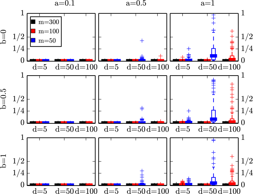
Figure 4: The boxplots summarise the results of $100$ experiments running MERLiN${}_{\Sigma^{-1}}$ on datasets $\mathcal{{D}}_{T}^{d\times m}(a,b)$ for $T=G$ (cf. Section IV-A). The performance measure $\operatorname{pobv}_{\bm{w}_{G0}}(\bm{w})$ is shown on the $y$-axes and described in Section IV-B (low values are good). The box for $d=100,m=50$ is missing since MERLiN${}_{\Sigma^{-1}}$ can only be applied if $d\leq m$.

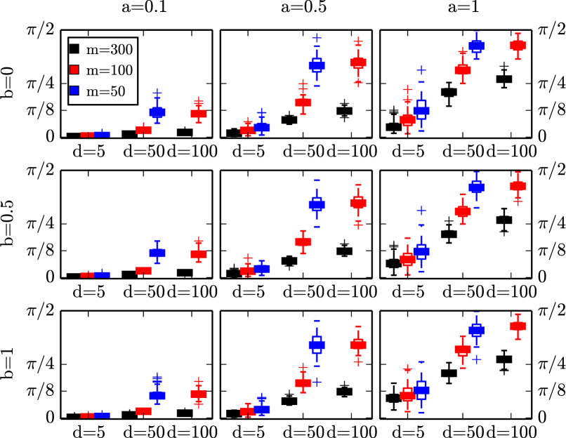
Figure 5: The boxplots summarise the results of $100$ experiments running MERLiN${}_{\Sigma^{-1}}$ on datasets $\mathcal{{D}}_{T}^{d\times m}(a,b)$ for $T=G$ (cf. Section IV-A). The performance measure $\operatorname{andi}_{\bm{w}_{G0}}(\bm{w})$ is shown on the $y$-axes and described in Section IV-B (low values are good). The box for $d=100,m=50$ is missing since MERLiN${}_{\Sigma^{-1}}$ can only be applied if $d\leq m$.

V How to extend MERLiN

In this section we demonstrate how the basic MERLiN algorithm can be extended to enable application to different data modalities by (a) including data specific preprocessing steps into the optimisation procedure (cf. Section V-A), and (b) incorporating a priori domain knowledge (cf. Section V-B). In particular, we demonstrate this for neuroimaging data, since stimulus-based experiments pose a prototype application scenario for MERLiN for the following reasons.

1. In stimulus-based experiments the stimulus $S$ is randomised, meeting the assumption in Section III-A1 [11].

2. Recent work in the neuroimaging community focusses on functional networks, i. e., a (linear) combination of activity spread across the brain that is functionally (read causally) relevant [29]. Additionally, the recorded activity is often assumed to be a linear combination of underlying cortical variables, as for example in EEG [2].

3. Simple univariate methods suffice to identify an effect $C_{1}$ of $S$ [12, Interpretation rule S1].

The proposed method can readily be applied and complement the standard analysis procedures employed in such experiments. More precisely, MERLiN can recover meaningful cortical networks (read causal variables) that are causally affected by $C_{1}$, thereby establishing a cause-effect relationship between two functional brain state features.

V-A MERLiN${}_{\Sigma^{-1}}^{bp}$: adaptation to EEG data

Analyses of EEG data commonly focus on trial-averaged log-bandpower in a particular frequency band. Accordingly, we aim at identifying a linear combination of electrode signals such that the trial-averaged log-bandpower of the recovered signal is indirectly affected by the stimulus via another predefined cortical signal. We demonstrate how to do so by extending the basic MERLiN algorithm to include the log-bandpower computation into the optimisation procedure.

More precisely, we consider EEG trial-data of the form $\widetilde{\bm{F}}\in\mathbb{R}^{d\times m\times n}$ where $d$ denotes the number of electrodes, $m$ the number of trials, and $n$ the length of the time series $\widetilde{\bm{F}}_{i,j,1:n}$ for each electrode $i\in\mathbb{N}_{1:d}$ and each sample $j\in\mathbb{N}_{1:m}$. The aim is to identify a linear combination $\bm{w}\in\mathbb{R}^{d\times 1}$ such that the log-bandpower of the resulting one-dimensional trial signals $\bm{w}^{\top}\widetilde{\bm{F}}_{1:d,j,1:n}$ is a causal effect of the log-bandpower of the one-dimensional trial signals $\bm{v}^{\top}\widetilde{\bm{F}}_{1:d,j,1:n}$. However, since the two operations of computing the log-bandpower (after windowing) and taking a linear combination do not commute, we cannot compute the trial-averaged log-bandpower for each channel first and then apply the standard precision matrix based MERLiN${}_{\Sigma^{-1}}$ algorithm. Instead, MERLiN${}_{\Sigma^{-1}}^{bp}$ has been adapted to the analysis of EEG data by switching in the log-bandpower computation.

To simplify the optimisation loop we exploit the fact that applying a Hanning window and the FFT to each channel’s signal commutes with taking a linear combination of the windowed and Fourier transformed time series. Note that averaging of the log-moduli ($\log(|\cdot|)$) of the Fourier coefficients does not commute with taking a linear combination. Hence, windowing and computing the FFT is done in a separate preprocessing step (cf. Algorithm 3), while the trial-averaged bandpower is computed within the optimisation loop after taking the linear combination. Implementation details for the bandpower and precision matrix based MERLiN${}_{\Sigma^{-1}}^{bp}$ algorithm are described in Algorithm 4. To ease implementation we treat the complex numbers as two-dimensional vector space over the reals.

Algorithm 3 Preprocessing for bp algorithm.

Input: $\bm{S}\in\mathbb{R}^{m\times 1},\widetilde{\bm{F}}\in\mathbb{R}^{d\times m\times n},\bm{v}\in\mathbb{R}^{d\times 1}$, the sampling frequency $f_{s}$, and the desired frequency range defined by $\omega_{1}$ and $\omega_{2}$

Procedure:

• set $a:=\lfloor\frac{\omega_{1}n}{f_{s}}\rfloor$, $b:=\lfloor\frac{\omega_{2}n}{f_{s}}\rfloor$, and $n^{\prime}:=b-a+1$

• for $i$ from $1$ to $d$, for $j$ from $1$ to $m$

  • center, apply Hanning window and compute FFT, i. e., treat $\widetilde{\bm{F}}_{i,j,1:n}$ as a column vector and set $\widetilde{\bm{F}}_{i,j,1:n}:=\bm{TW}\bm{H}_{n}\widetilde{\bm{F}}_{i,j,1:n}$

• extract relevant Fourier coefficients corresponding to $\bm{v}$, i. e., set

  $$\bm{V}^{\operatorname{Im}}:= \operatorname{Im}\left(\bm{v}^{\top}\widetilde{\bm{F}}_{1:d,j,a:b}\right)_{j=1:m}\in\mathbb{R}^{m\times n^{\prime}}$$

  $$\bm{V}^{\operatorname{Re}}:= \operatorname{Re}\left(\bm{v}^{\top}\widetilde{\bm{F}}_{1:d,j,a:b}\right)_{j=1:m}\in\mathbb{R}^{m\times n^{\prime}}$$

• remove direction $\bm{v}$ from $\widetilde{\bm{F}}$, i. e., for $j$ from $1$ to $m$ set

  $$\bm{F}_{1:(d-1),j,1:n^{\prime}}^{\operatorname{Im}}:= \operatorname{Im}\left(P(\bm{v})\widetilde{\bm{F}}_{1:d,j,a:b}\right)\in\mathbb{R}^{(d-1)\times n^{\prime}}$$

  $$\bm{F}_{1:(d-1),j,1:n^{\prime}}^{\operatorname{Re}}:= \operatorname{Re}\left(P(\bm{v})\widetilde{\bm{F}}_{1:d,j,a:b}\right)\in\mathbb{R}^{(d-1)\times n^{\prime}}$$

  such that $\bm{F}^{\operatorname{Im}},\bm{F}^{\operatorname{Re}}\in\mathbb{R}^{(d-1)\times m\times n^{\prime}}$

Output: $\bm{V}^{\operatorname{Im}},\bm{V}^{\operatorname{Re}}\in\mathbb{R}^{m\times n^{\prime}}$ and $\bm{F}^{\operatorname{Im}},\bm{F}^{\operatorname{Re}}\in\mathbb{R}^{(d-1)\times m\times n^{\prime}}$

 

Definitions:

• $P(\bm{v})$ is the $(d-1)\times d$ orthonormal matrix that accomplishes projection onto the orthogonal complement $\bm{v}_{\perp}$

• $\bm{H}_{n}=\bm{I}_{n\times n}-\frac{1}{n}\bm{1}_{n\times n}$ is the $n\times n$ centering matrix

• $\bm{W}=\left[\frac{1}{2}\left(1-\cos\frac{2\pi k}{n-1}\right)\right]_{k,l=1:n}$ is the $n\times n$ Hanning window matrix

• $\bm{T}=\left[\exp\left(-\imath 2\pi k\frac{l}{n}\right)\right]_{k,l=1:n}$ is the $n\times n$ FFT matrix

Algorithm 4 MERLiN${}_{\Sigma^{-1}}^{bp}$

Refer to Algorithm 5 and instead use the objective function

$$f(\bm{w})=\left|\left(\widehat{\Sigma}_{\bm{w}}^{-1}\right)_{2,3}\right|-\left|\left(\widehat{\Sigma}_{\bm{w}}^{-1}\right)_{1,3}\right|$$

V-B MERLiN${}_{\Sigma^{-1}}^{bp+}$: incorporating a priori knowledge

Here we demonstrate how to incorporate a priori domain knowledge by modifying the objective function of the MERLiN${}_{\Sigma^{-1}}^{bp}$ algorithm. Utilising a priori knowledge about volume conduction in EEG recordings results in the refined MERLiN${}_{\Sigma^{-1}}^{bp+}$ algorithm.

A cortical source projects into more than one EEG electrode. In general, these volume conduction artefacts might lead to wrong conclusions about interactions between sources [30]. Imaginary coherency, as introduced in [31], may help to differentiate volume conduction artefacts from interactions between cortical sources. To briefly recap the rationale, we employ the common assumption that the signals measured at the EEG electrodes have no time-lag to the cortical signals [32]. The coherency at a certain frequency of two time series $X$ and $Y$ with Fourier coefficients $x(j),y(j),j\in\mathbb{N}_{1:n}$ is defined as

$$\operatorname{coh}_{X,Y}(j)=\frac{\mathbb{E}\left[x(j)y^{*}(j)\right]}{\sqrt{\mathbb{E}\left[x(j)x^{*}(j)\right]\mathbb{E}\left[y(j)y^{*}(j)\right]}}$$

where ^∗ denotes complex conjugation. Next consider the coherency of $X$ and $Y+X$

$\operatorname{coh}_{X,Y+X}=\frac{\mathbb{E}\left[x(j)y^{*}(j)\right]+\mathbb{E}\left[x(j)x^{*}(j)\right]}{\sqrt{\mathbb{E}\left[x(j)x^{*}(j)\right]\mathbb{E}\left[\left(y(j)+x(j)\right)\left(y^{*}(j)+x^{*}(j)\right)\right]}}$

and observe that $\mathbb{E}\left[x(j),x^{*}(j)\right]$ is real. This shows that non-zero imaginary coherency $\operatorname{icoh}_{X,Y}(j)\triangleq\operatorname{Im}(\operatorname{coh}_{X,Y}(j))$ cannot be due to volume conduction and indicates time-lagged interaction between sources since it implies that $\operatorname{Im}(\mathbb{E}\left[x(j)y^{*}(j)\right])\neq 0$.

This a priori knowledge is incorporated in MERLiN${}_{\Sigma^{-1}}^{bp+}$ by adapting the objective function to be

$$f(\bm{w})=\left|\sum_{j=1}^{n^{\prime}}\operatorname{icoh}(j)\right|\cdot\left|\left(\widehat{\Sigma}_{\bm{w}}^{-1}\right)_{2,3}\right|-\left|\left(\widehat{\Sigma}_{\bm{w}}^{-1}\right)_{1,3}\right|$$

where $\widehat{\Sigma}_{\bm{w}}^{-1}$ denotes the empirical precision matrix of the log-bandpower features after taking the linear combination $\bm{w}$ and $\operatorname{icoh}(j)$ denotes the imaginary coherency between the signals corresponding to $\bm{v}$ and $\bm{w}$ estimated as average over all trials (cf. Algorithm 5 for details). While there are several ways of setting up the objective function we have chosen this multiplicative set-up as it quite naturally captures the following idea: whenever we find the resulting bandpower to be dependent on $C_{1}$ we also want to ensure that this is not just an artefact due to volume conduction. Note that this extension may also help disentangle true cortical sources, i. e., the causal variables, by avoiding a mixture of distinct sources affected by $C_{1}$ that have different time-lags and hence result in lower imaginary coherency.

Algorithm 5 MERLiN${}_{\Sigma^{-1}}^{bp+}$

Input: $\bm{S}\in\mathbb{R}^{m\times 1},\widetilde{\bm{F}}\in\mathbb{R}^{d\times m\times n},\bm{v}\in\mathbb{R}^{d\times 1}$, the sampling frequency $f_{s}$, and the desired frequency range defined by $\omega_{1}$ and $\omega_{2}$

Procedure:

• obtain $\bm{V}^{\operatorname{Im}},\bm{V}^{\operatorname{Re}}\in\mathbb{R}^{m\times n^{\prime}}$ and $\bm{F}^{\operatorname{Im}},\bm{F}^{\operatorname{Re}}\in\mathbb{R}^{d^{\prime}\times m\times n^{\prime}}$ via Algorithm 3 where $d^{\prime}=d-1$

• set $\bm{C}:=\left(\frac{1}{n^{\prime}}\sum_{j=1}^{n^{\prime}}\log_{*}\left(\frac{\sqrt{\left(\bm{V}_{i,j}^{\operatorname{Im}}\right)^{2}+\left(\bm{V}_{i,j}^{\operatorname{Re}}\right)^{2}}}{n}\right)\right)_{i=1:m}\in\mathbb{R}^{m\times 1}$ (average log-bandpower per trial)

• define the objective function for $\bm{w}\in O^{d-2}$ as

  $$f(\bm{w})=\left|\sum_{j=1}^{n^{\prime}}\operatorname{icoh}(j)\right|\cdot\left|\left(\widehat{\Sigma}_{\bm{w}}^{-1}\right)_{2,3}\right|-\left|\left(\widehat{\Sigma}_{\bm{w}}^{-1}\right)_{1,3}\right|$$

  where the empirical precision matrix is

  $$\widehat{\Sigma}_{\bm{w}}^{-1}=\left(\frac{1}{m-1}\left[\bm{S},\bm{C},\bm{D_{w}}\right]^{\top}\bm{H}_{m}\left[\bm{S},\bm{C},\bm{D_{w}}\right]\right)^{-1},$$

  the average log-bandpower per trial depending on $\bm{w}$ is
  $\bm{D_{w}}=\left(\frac{1}{n^{\prime}}\sum_{j=1}^{n^{\prime}}\log_{*}\left(\frac{\sqrt{\left(\bm{w}^{\top}\bm{F}_{1:d^{\prime},i,j}^{\operatorname{Im}}\right)^{2}+\left(\bm{w}^{\top}\bm{F}_{1:d^{\prime},i,j}^{\operatorname{Re}}\right)^{2}}}{n}\right)\right)_{i=1:m}\in\mathbb{R}^{m\times 1},$ and the imaginary coherency $\operatorname{icoh}(j)$ for each frequency $j\in\mathbb{N}_{1:n^{\prime}}$ equals
  $\frac{\left\langle\bm{V}_{i,j}^{\operatorname{Im}}\cdot\bm{w}^{\top}\bm{F}_{1:d^{\prime},i,j}^{\operatorname{Re}}-\bm{V}_{i,j}^{\operatorname{Re}}\cdot\bm{w}^{\top}\bm{F}_{1:d^{\prime},i,j}^{\operatorname{Im}}\right\rangle_{i=1:m}}{\sqrt{\left\langle\left(\bm{V}_{i,j}^{\operatorname{Im}}\right)^{2}+\left(\bm{V}_{i,j}^{\operatorname{Re}}\right)^{2}\right\rangle_{i=1:m}\left\langle\left(\bm{w}^{\top}\bm{F}_{1:d^{\prime},i,j}^{\operatorname{Im}}\right)^{2}+\left(\bm{w}^{\top}\bm{F}_{1:d^{\prime},i,j}^{\operatorname{Re}}\right)^{2}\right\rangle_{i=1:m}}}$

• optimise $f$ as described in Section II-B to obtain the vector $\bm{w}^{*}\in O^{d-2}$

Output: $\bm{w}=P(\bm{v})^{\top}\bm{w}^{*}\in O^{d-1}$

 

Definitions:

• $P(\bm{v})$ is the $(d-1)\times d$ orthonormal matrix that accomplishes projection onto the orthogonal complement $\bm{v}_{\perp}$

• $\bm{H}_{m}=\bm{I}_{m\times m}-\frac{1}{m}\bm{1}_{m\times m}$ is the $m\times m$ centering matrix

• $\log_{*}$ is the extended log function with $\log_{*}(x)=\log(x),\ x>0$ and $\log_{*}(0)=0$

• the notation$\langle\cdot\rangle_{i=1:m}$ denotes the empirical mean, i. e., $\langle a_{i}\rangle_{i=1:m}=\frac{1}{m}\sum_{i=1}^{m}a_{i}$

VI Experiments on empirical EEG data

VI-A Sanity check of the included log-bandpower computation

We ran simulation experiments with the MERLiN${}_{\Sigma^{-1}}^{bp}$ algorithm analogous to those presented in Section IV. For this we used datasets $\mathcal{TD}_{T}^{d\times m\times n}(a,b)$ that are generated from $\mathcal{D}_{T}^{d\times m}(a,b)$ with fixed mixing matrix $\bm{A}=\bm{I}_{d\times d}$ as follows. While $\bm{S},\bm{v},\bm{w}_{G0}$ remain unchanged the $d\times m$ matrix $\bm{F}$ is replaced by a $d\times m\times n$ tensor $\widetilde{\bm{F}}$ that consists of $dm$ chunks of randomly chosen real EEG signals of length $n$. Each signal $\widetilde{\bm{F}}_{i,j,1:n}$ is modified such that the log-bandpower in the desired frequency band equals $\bm{F}_{i,j}$.

The log-bandpower computation was incorporated into the algorithm in such a way that the optima for MERLiN${}_{\Sigma^{-1}}^{bp}$ on $\mathcal{TD}_{T}^{d\times m\times n}(a,b)$ coincide with those for MERLiN${}_{\Sigma^{-1}}$ on the corresponding dataset $\mathcal{D}_{T}^{d\times m\times n}(a,b)$; however, the shape of the objective functions is different. Accordingly and as expected, sanity checks of MERLiN${}_{\Sigma^{-1}}^{bp}$ on $\mathcal{TD}_{T}^{d\times m\times n}(a,b)$ show trends for varying parameters $T,d,m,a,b$ similar to those discussed in Section IV-C.

VI-B Description of empirical data

We next evaluate MERLiN with EEG data recorded during a neurofeedback experiment [33]. Subjects in this study were instructed in pseudo-randomised order to up- or down-regulate the amplitude of $\gamma$-oscillations ($55$–$85$ Hz) in the right superior parietal cortex (SPC). For the feedback the activity in the SPC was extracted by a linearly-constrained-minimum variance (LCMV) beamformer [34] that was trained on $5$ min resting-state EEG data.

Each recording session ($3$ subjects a $2$ sessions referred to as S1R1, S1R2, S2R1, …) consists of $60$ trials of $60$ seconds each. The stimulus variable $S$ is either $+1$ or $-1$ depending on whether the subject was instructed to up- or down-regulate $\gamma$-power in the SPC. Electromagnetic artefacts were attenuated as described in [33, Section 2.4.1] and the EEG data downsampled to $250$ Hz. We are also given the spatial filter $\bm{v}\in\mathbb{R}^{121\times 1}$ for each session, i. e., the beamformer that was used to extract the feedback signal. Thus, the data of one session can be arranged as $\bm{S}\in\{-1,+1\}^{60\times 1},\bm{v}\in\mathbb{R}^{121\times 1}$ and $\widetilde{\bm{F}}\in\mathbb{R}^{121\times 60\times 15000}$ where $\widetilde{\bm{F}}$ contains the timeseries (of length $15000$) for each channel and trial.

VI-C Assessing MERLiN’s performance

MERLiN’s performance on these data is assessed by comparing against results from an earlier exhaustive search approach. The hypothesis in [17] is that $\gamma$-oscillations in the SPC modulate $\gamma$-oscillations in the medial prefrontal cortex (MPFC) and was derived from previous transcranial magnetic stimulation studies [35]. In order to test this hypothesis, the signal of $K\triangleq 15028$ dipoles across the cortical surface was extracted using a LCMV beamformer and a three-shell spherical head model [36]. The SCI algorithm was used to assess for every dipole whether its $\gamma$-log-bandpower is a causal effect of the $\gamma$-log-bandpower in the SPC. This analysis confirmed the MPFC as a causal effect of the SPC (cf. Figure 6).

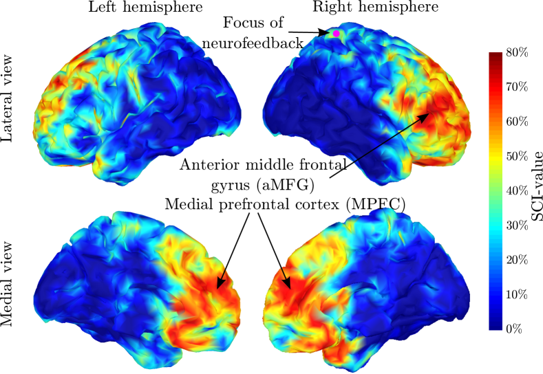
Figure 6: Figure adapted from [17]. The neurofeedback target area in the right SPC is indicated by a pink circle. The SCI value denotes the percentage of dipoles within a radius of 7 mm that were found to be modulated by the SPC. From these results, the authors inferred the primary targets of the right SPC to be the MPFC and additionally the right aMFG.

To allow comparison against these results we derive a vector $\bm{g}\in\mathbb{R}^{K\times 1}$ that represents the involvement of each cortical dipole in the signal identified by MERLiN${}_{\Sigma^{-1}}^{bp+}$ as the linear combination $\bm{w}$ of electrode signals. A scalp topography is readily obtained via $\bm{a}\propto\Sigma\bm{w}$ where the $i^{\text{th}}$ entry of $\Sigma\bm{w}$ is the covariance between the $i^{\text{th}}$ EEG channel and the source that is recovered by $\bm{w}$ [37, Equation (7)]. Here $\Sigma$ denotes the subject-specific covariance matrix in the $\gamma$-frequency band. A dipole involvement vector $\bm{g}$ is obtained from $\bm{a}$ via dynamic statistical parametric mapping (dSPM; with the identity as noise covariance matrix) [38]. The resulting vectors are expected to be in line with previous findings and the hypothesis that the MPFC is affected by the SPC.

VI-D Experimental results

We applied MERLiN${}_{\Sigma^{-1}}^{bp+}$ several times, i. e., with different random initialisations, to the data of each of the $6$ sessions. We found that the $\gamma$-activation maps $\bm{a}$ obtained for each spatial filter $\bm{w}$ were (a) rather smooth and similar to what is typically assumed to be neurophysiologically plausible [39], and (b) consistent across different initialisations within sessions. The group average and individual dipole involvement vectors are shown in Figure 7, and Table I shows the resulting absolute (partial) correlations between $\gamma$-bandpower in the SPC ($C_{1}$), the $\gamma$-bandpower of the signal $\bm{w}^{\top}F$ identified by the MERLiN${}_{\Sigma^{-1}}^{bp+}$ algorithm ($C_{2}$), and the instruction to up- or down-regulate the $\gamma$-bandpower in the SPC ($S$).

Our results are in line with the previous findings (cf. Figure 6) inasmuch as they support the hypothesis that the MPFC is a causal effect of the SPC, i. e., $S\to C_{1}\to C_{2}$. We observe the following:

• For five out of six sessions and on group average the MPFC shows up as being causally affected by the SPC.

• Comparing the marginal correlation $\rho_{S,C_{2}}$ to the partial correlation $\rho_{S,C_{2}|C_{1}}$ suggests that indeed $C_{1}$ screens off $S$ and $C_{2}$, which is incompatible with the causal graph $C_{1}\leftarrow S\to C_{2}$. Recall that $C_{2}\centernot\mathchoice{\mathrel{\hbox to0.0pt{$\displaystyle\perp$\hss}\mkern 2.0mu{\displaystyle\perp}}}{\mathrel{\hbox to0.0pt{$\textstyle\perp$\hss}\mkern 2.0mu{\textstyle\perp}}}{\mathrel{\hbox to0.0pt{$\scriptstyle\perp$\hss}\mkern 2.0mu{\scriptstyle\perp}}}{\mathrel{\hbox to0.0pt{$\scriptscriptstyle\perp$\hss}\mkern 2.0mu{\scriptscriptstyle\perp}}}C_{1}$ and $C_{2}\mathchoice{\mathrel{\hbox to0.0pt{$\displaystyle\perp$\hss}\mkern 2.0mu{\displaystyle\perp}}}{\mathrel{\hbox to0.0pt{$\textstyle\perp$\hss}\mkern 2.0mu{\textstyle\perp}}}{\mathrel{\hbox to0.0pt{$\scriptstyle\perp$\hss}\mkern 2.0mu{\scriptstyle\perp}}}{\mathrel{\hbox to0.0pt{$\scriptscriptstyle\perp$\hss}\mkern 2.0mu{\scriptscriptstyle\perp}}}S|C_{1}$ are sufficient to uniquely infer $S\to C_{1}\to C_{2}$ (cf. Section III-B).

• Unlike the results in [17], the anterior middle frontal gyrus does not show up in Figure 7.

• The parietal/posterior cingulate cortex shows up for sessions S1R1 –here in addition to the MPFC– and for session S3S2.

Note that we used MERLiN to recover only one causal variable and hence, that the results are not expected to exactly resemble the exhaustive search results in [17]. If the true underlying graph is as depicted in Figure 8, then MERLiN may recover any combination $aC_{2}+bC_{3}$ as causal effect of $C_{1}$. This may explain both why the anterior middle frontal gyrus does not show up in our analysis –MERLiN recovering only one effect, namely $C_{2}$ but not $C_{3}$– and the lack of intra-subject consistency –slight inter-session differences may lead to recovery of different combinations of effects of $C_{1}$. Also note that if the assumption of orthogonal mixing is violated the SPC signal can only be attenuated but not removed (cf. Section III-C). This may explain the outlier result for session S3R2: The high correlation between $C_{1}$ and $C_{2}$ indicates that essentially the SPC signal was recovered, i. e., $C_{1}\approx C_{2}$.

Group average

Left hemisphere 

Lateral view

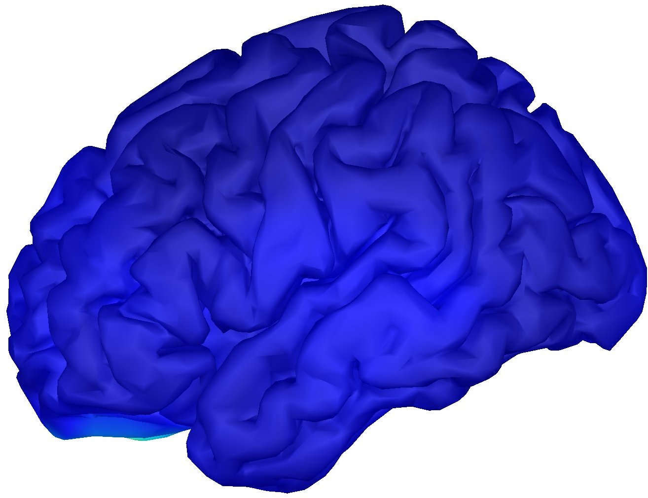
Right hemisphere

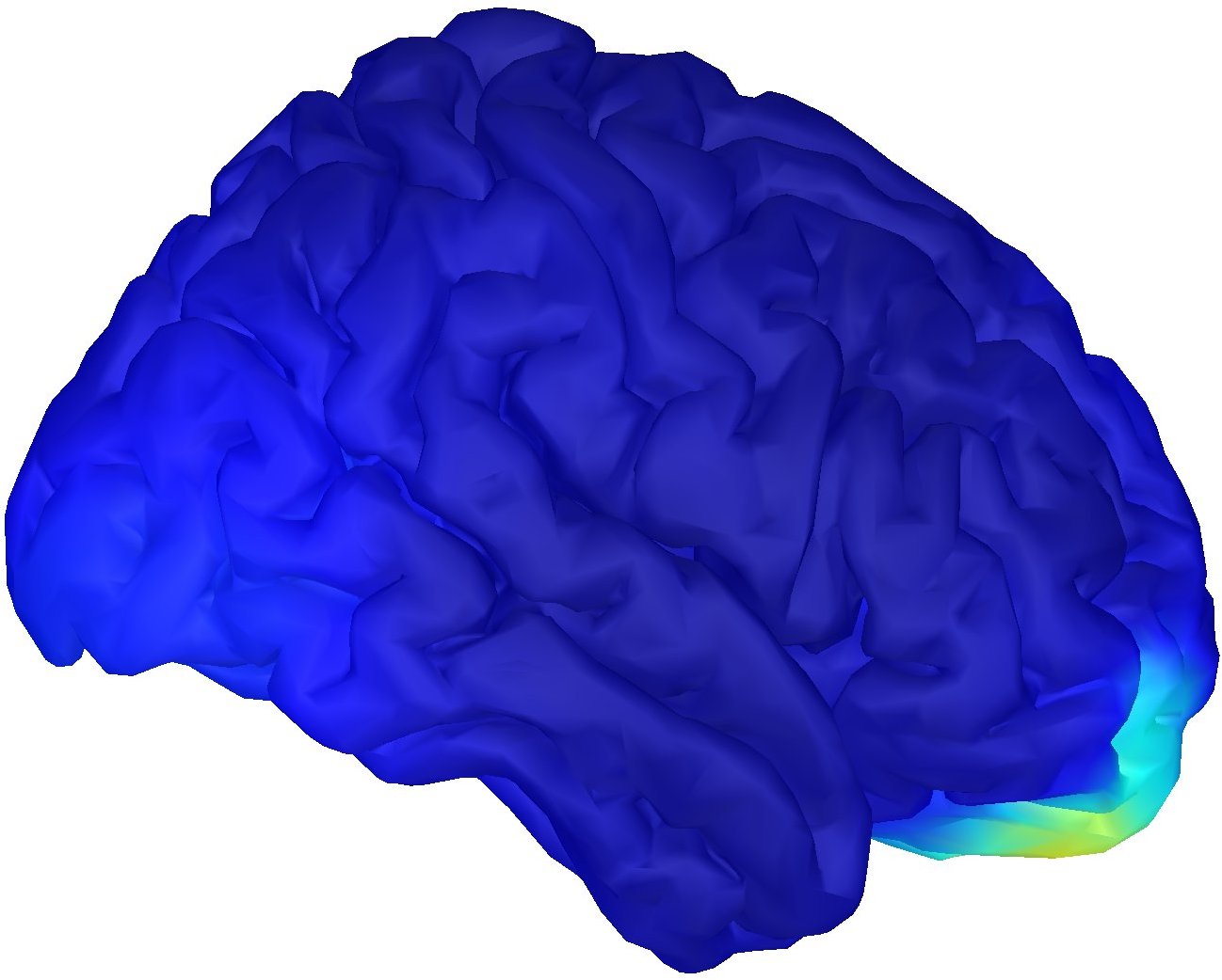
Medial view

 

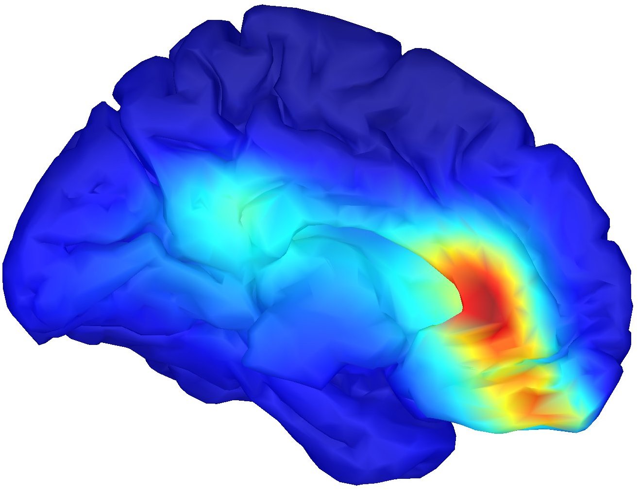
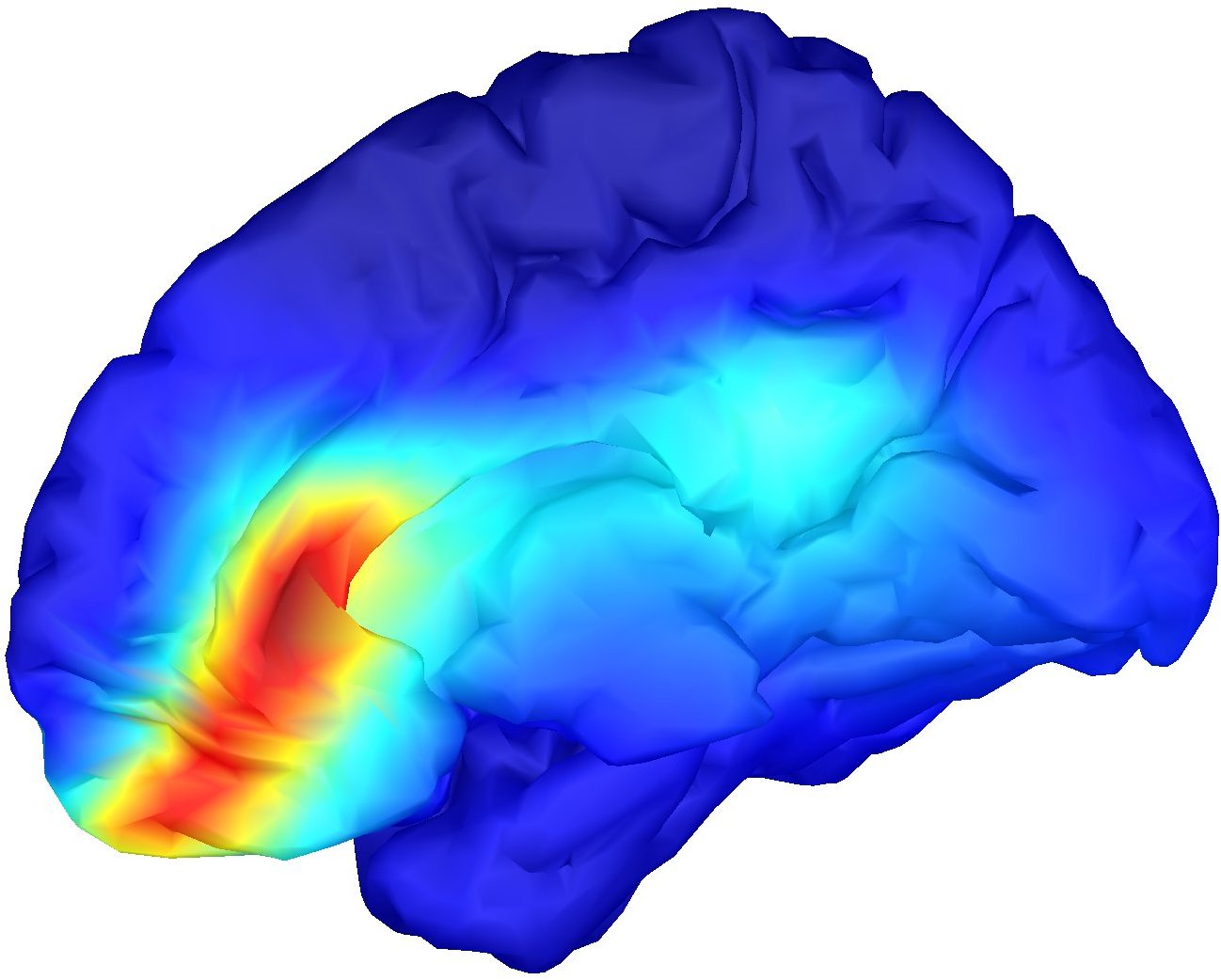
S1R1

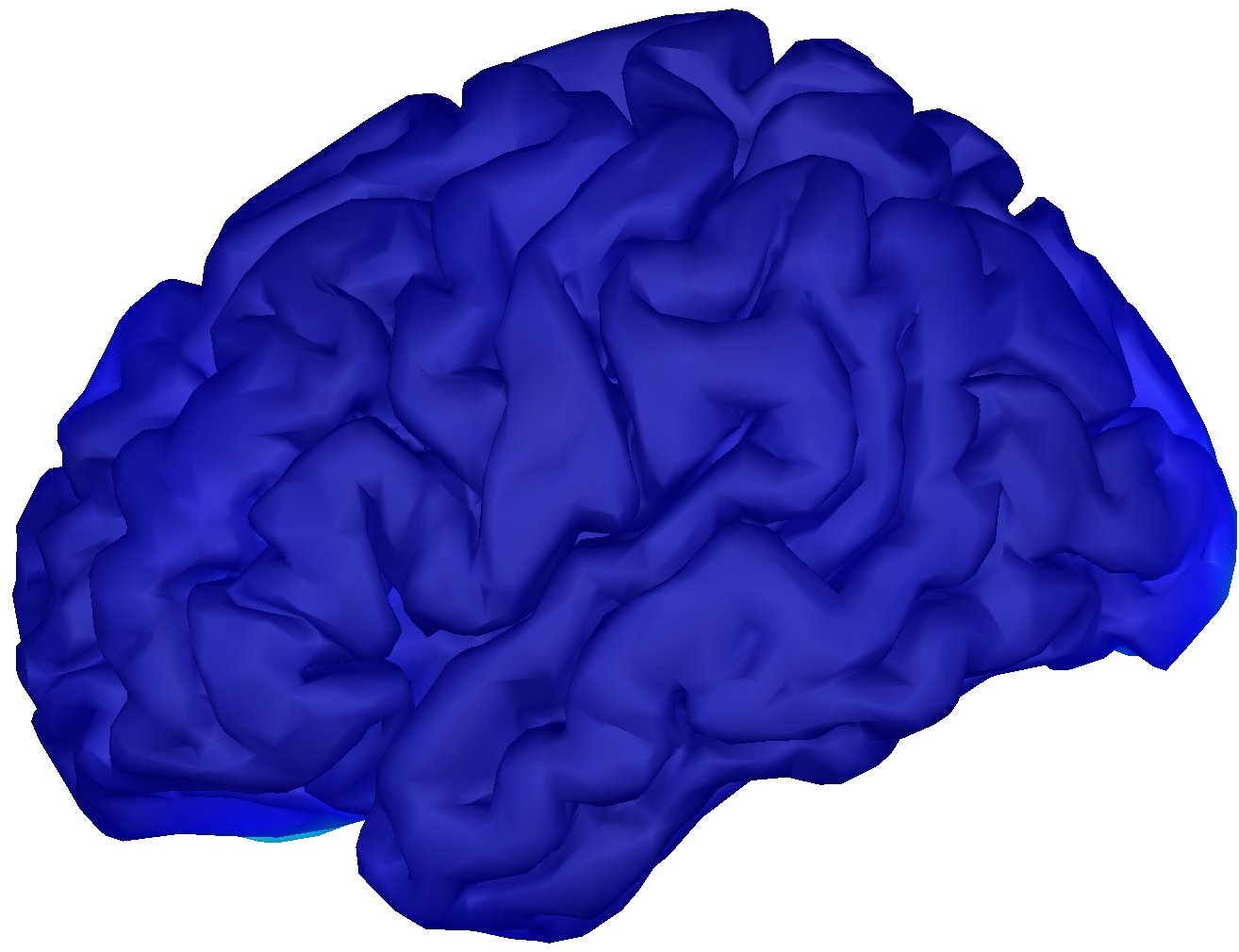
1

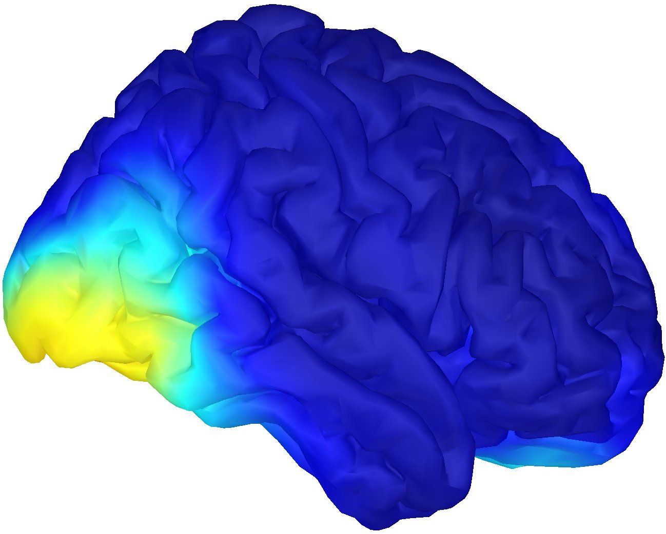
S1R2

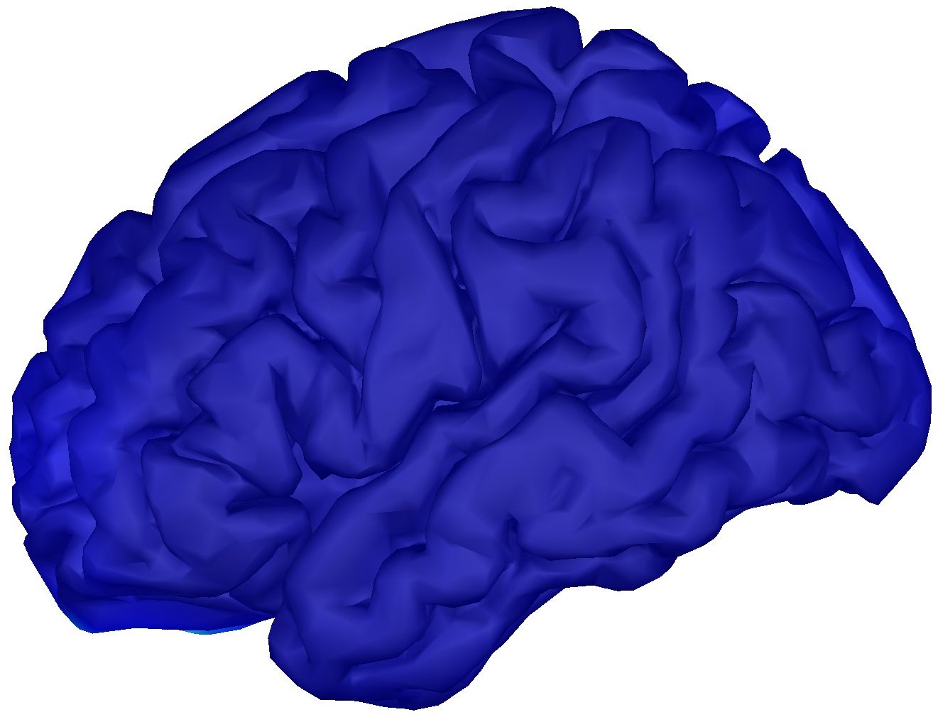
1

 

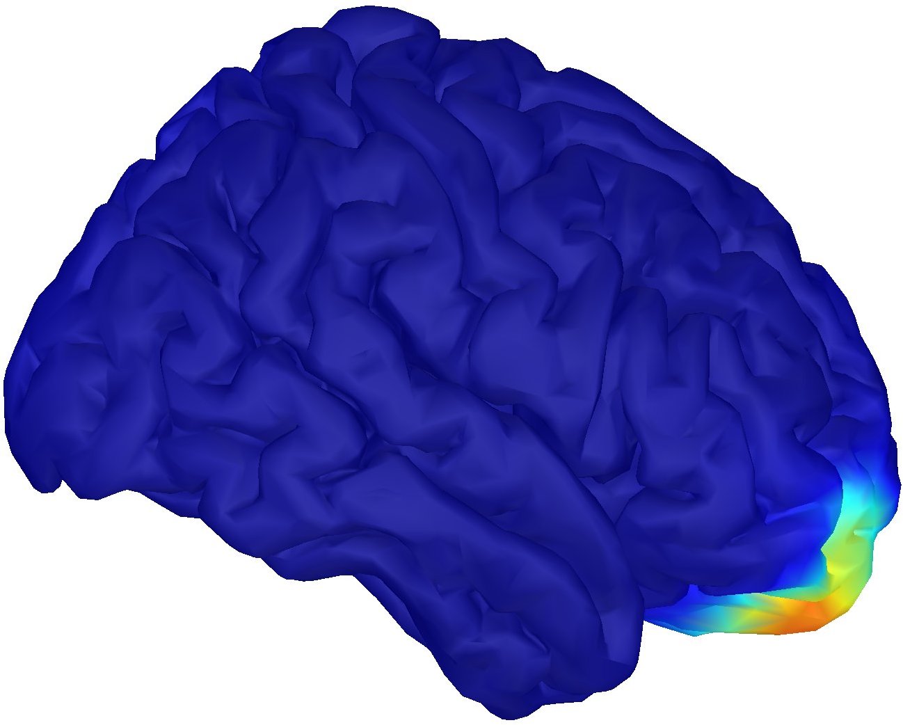
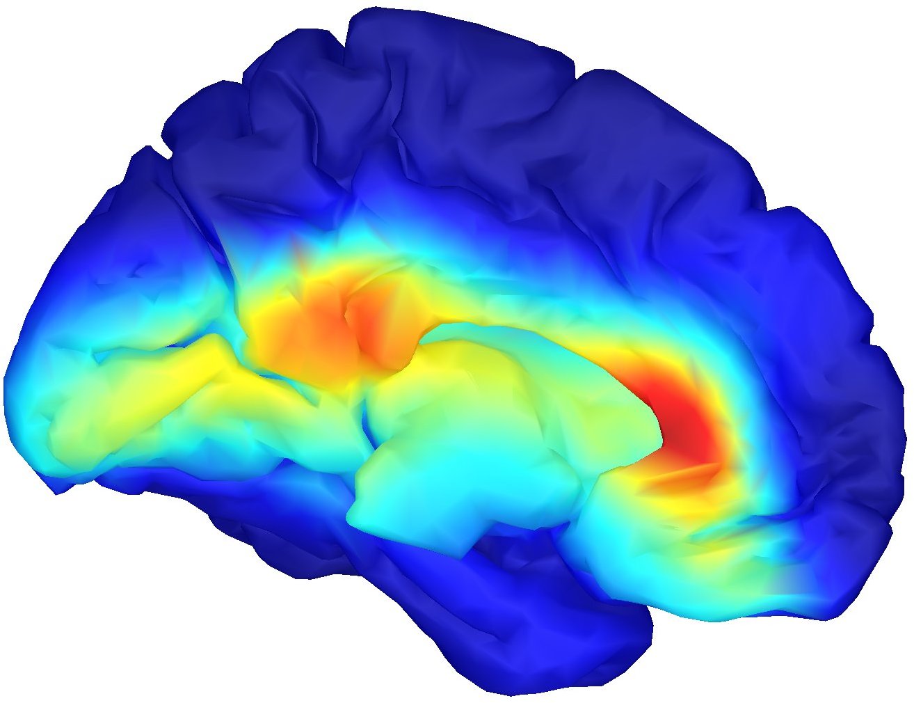
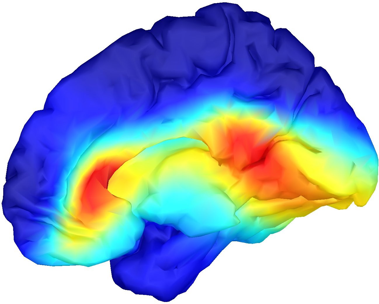
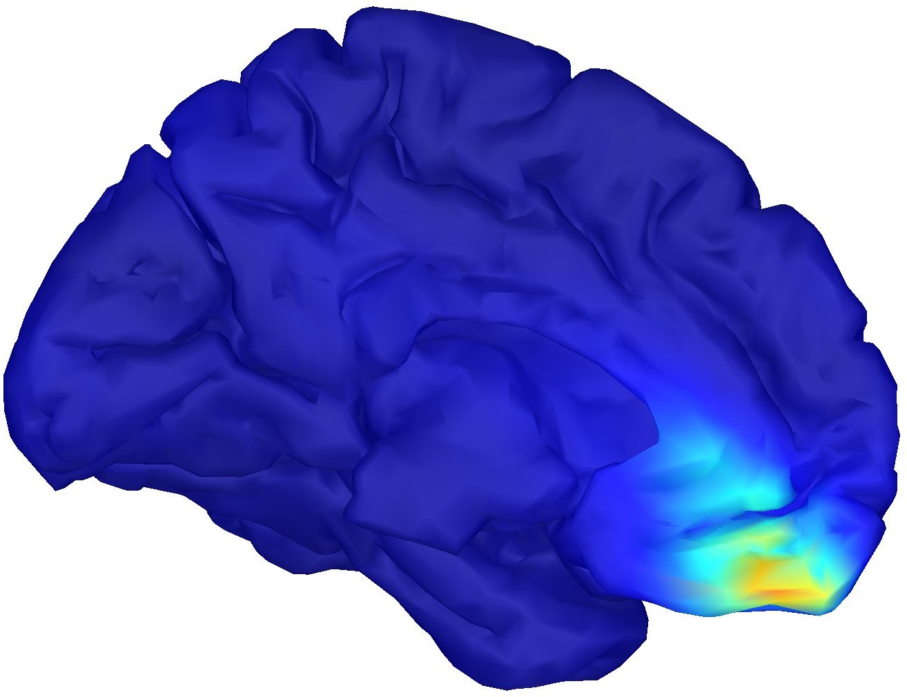
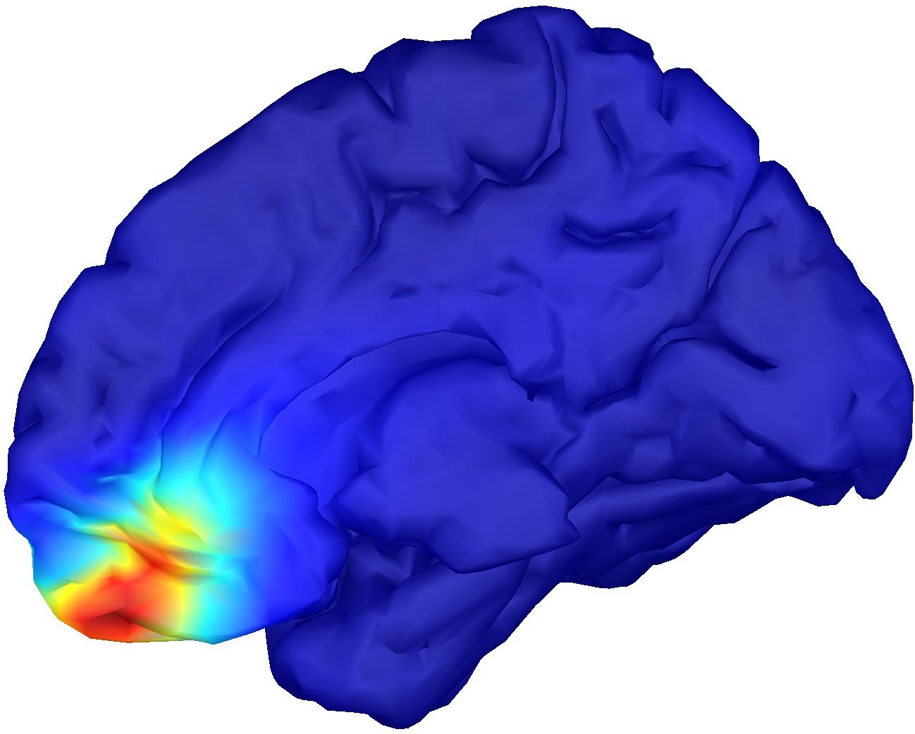
S2R1

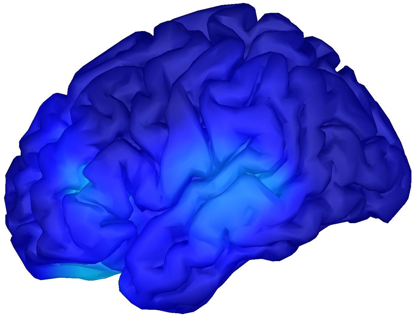
1

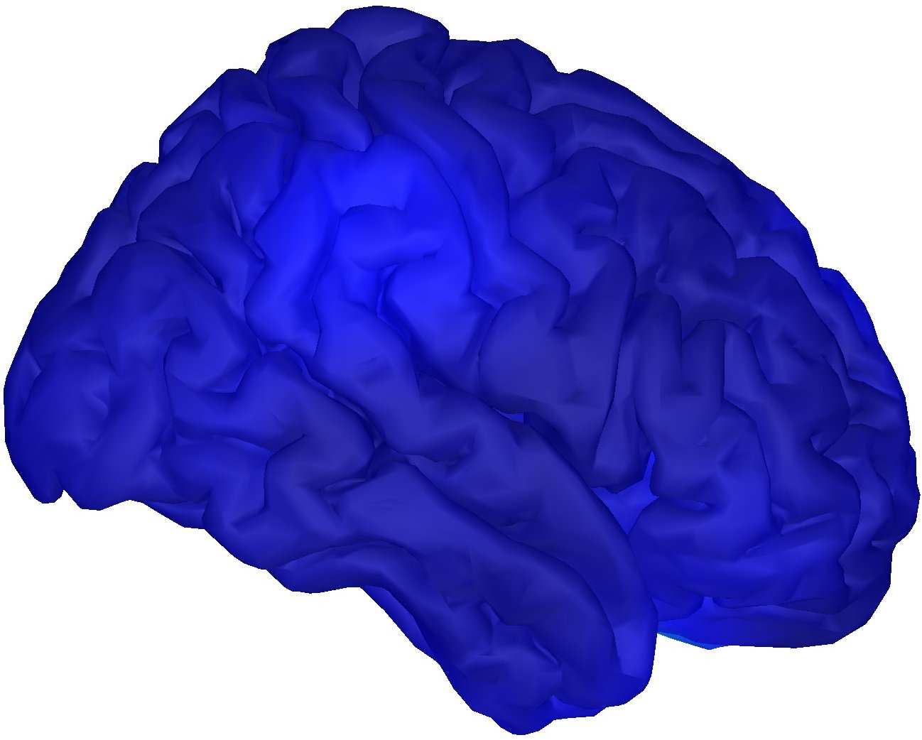
S2R2

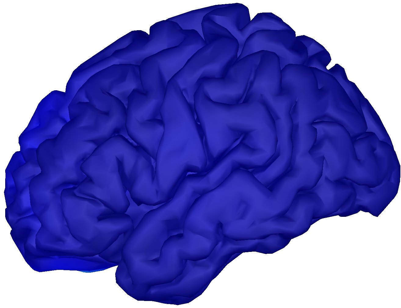
1

 

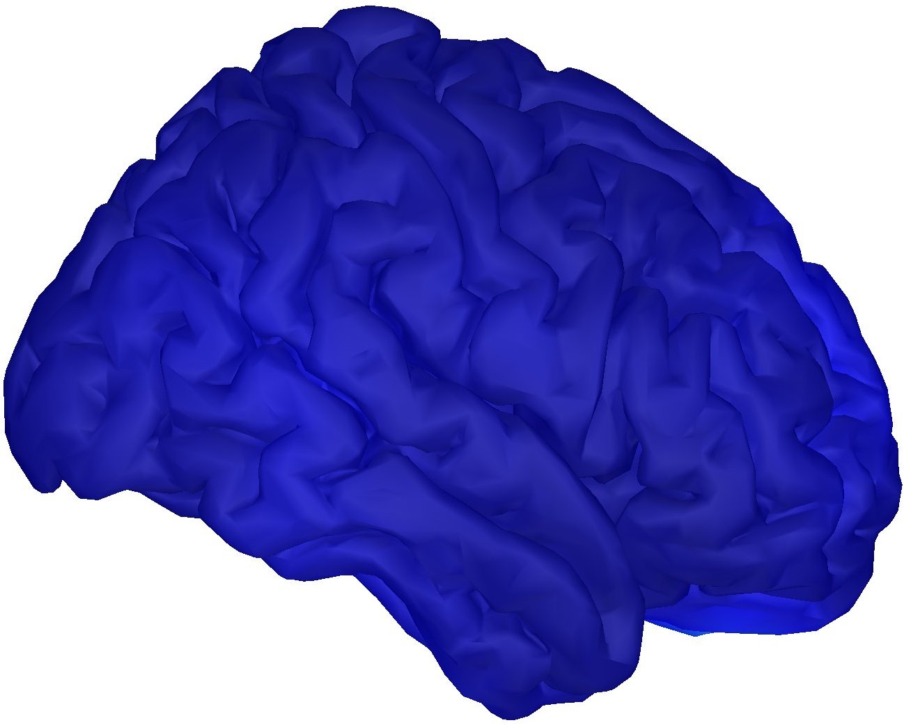
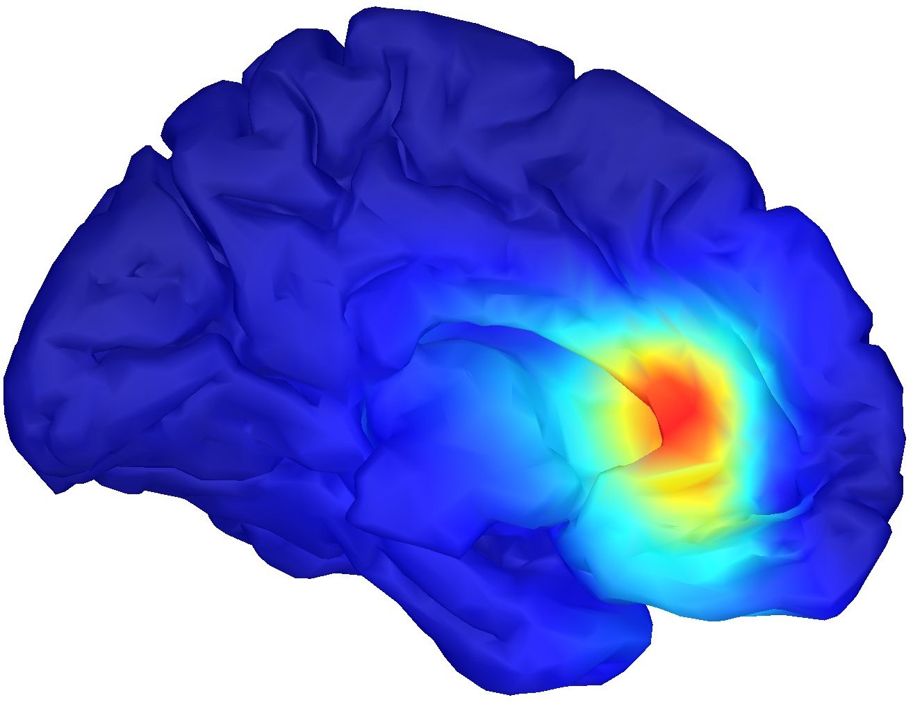
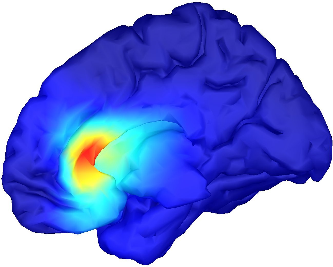
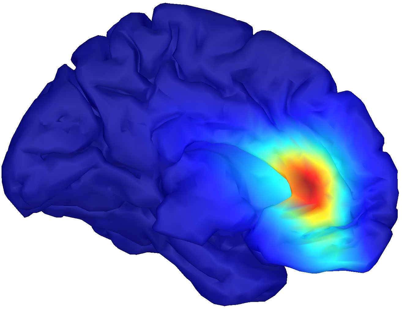
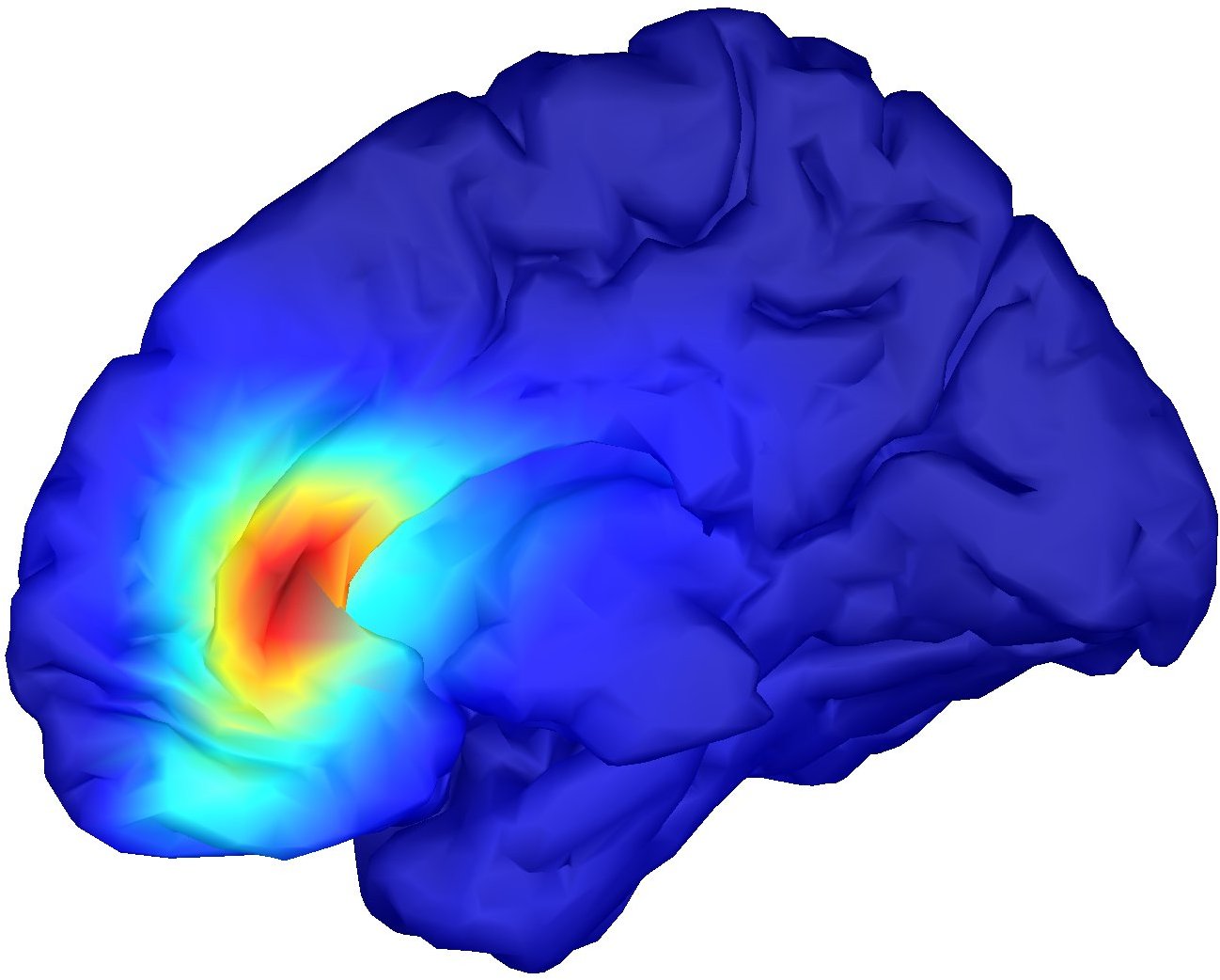
S3R1

1

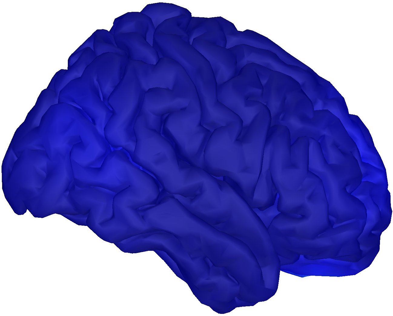
S3R2

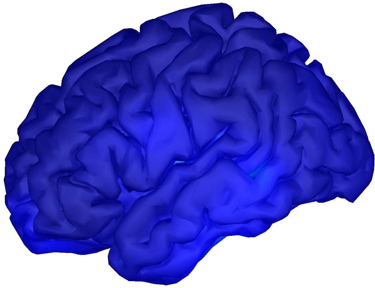
1

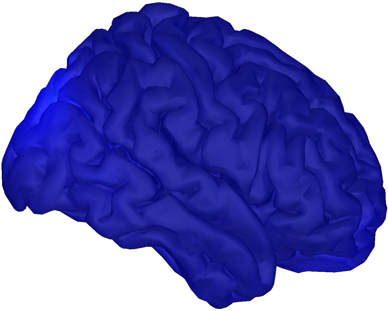
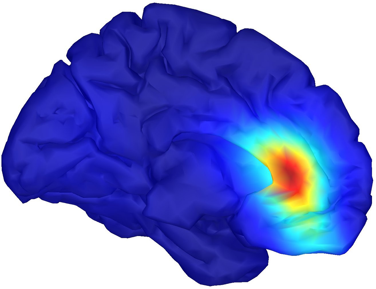
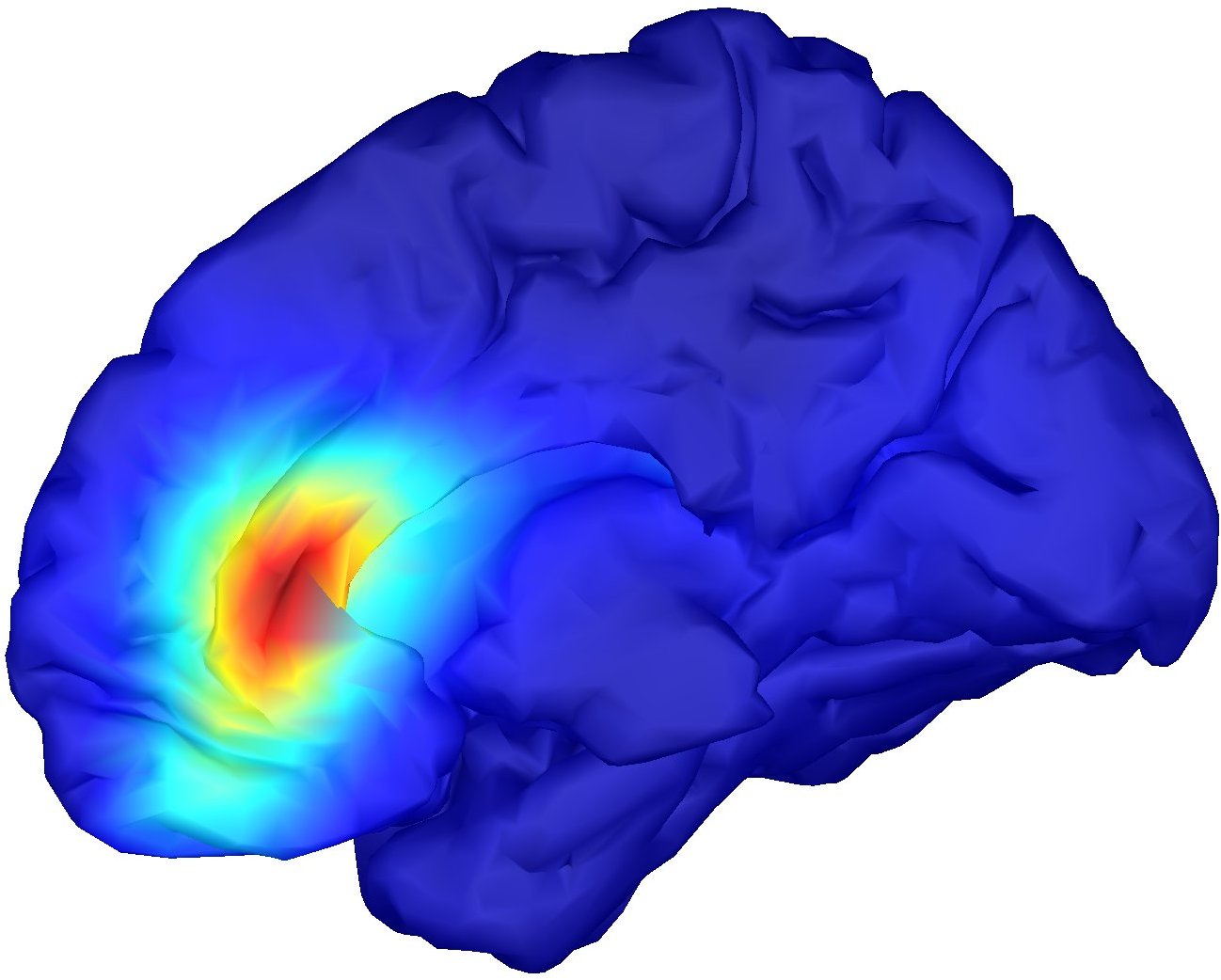
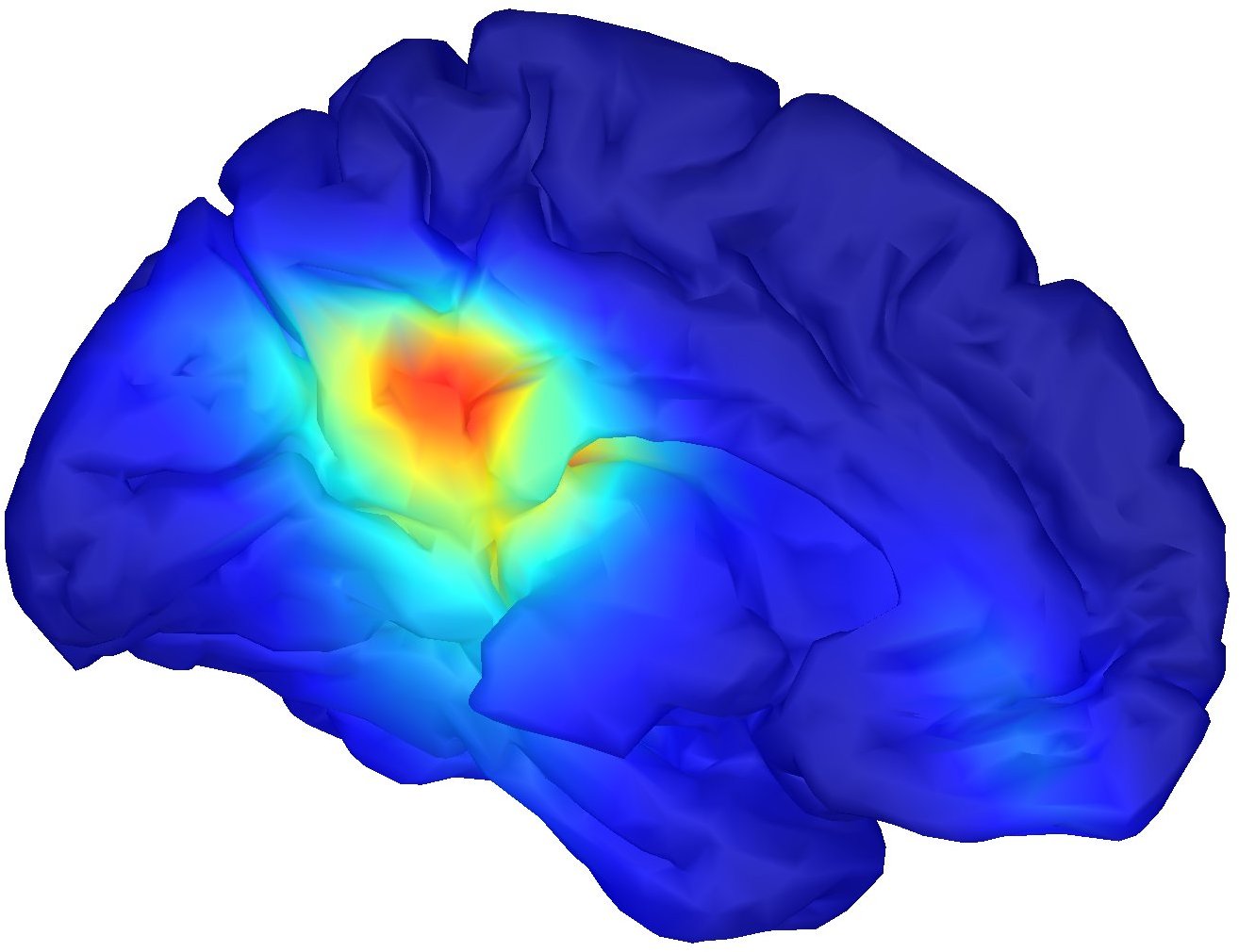
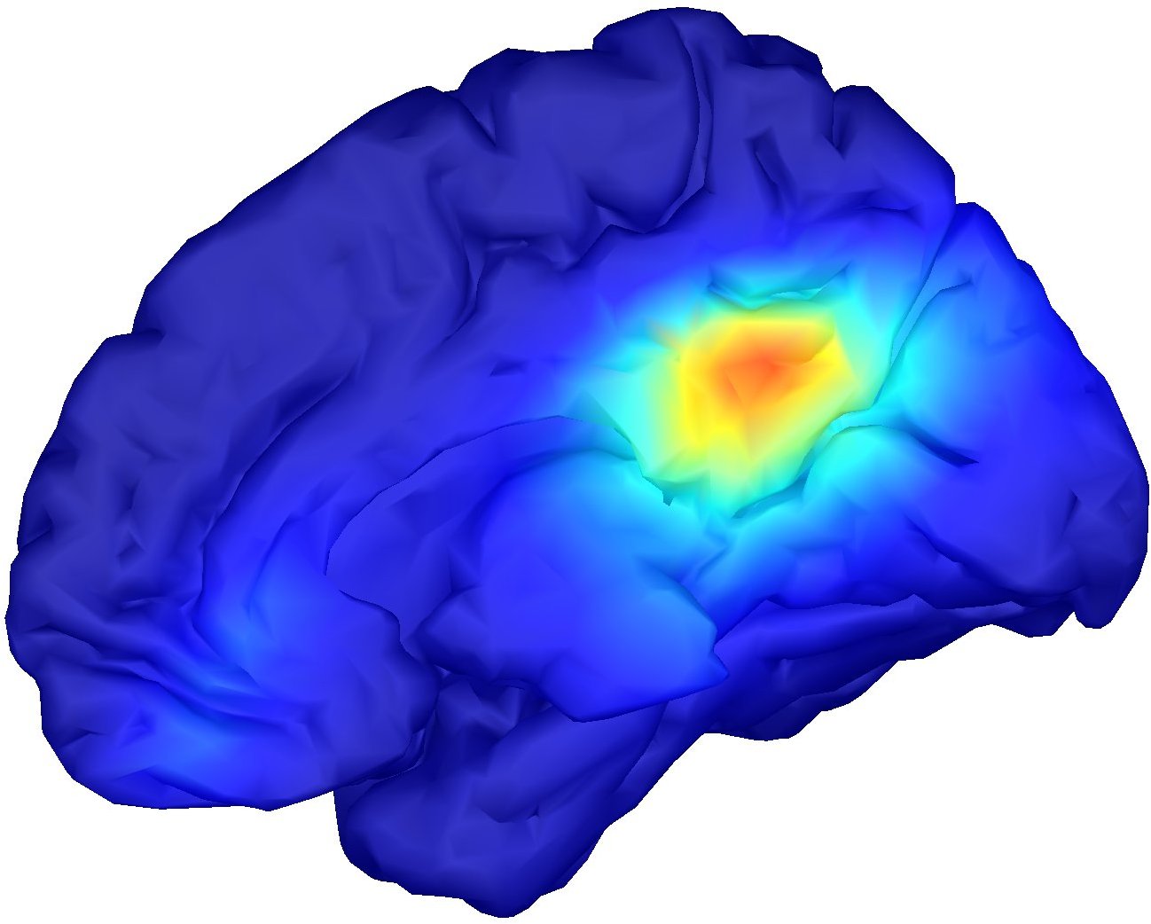
Figure 7: Spatial pattern of the effect of the SPC as identified by MERLiN${}_{\Sigma^{-1}}^{bp+}$. Group average (first row) and for individual sessions (bottom rows). Each subplot consists of a lateral (top) and medial (bottom) view of the left (left) and right (right) hemisphere. (All colorscales from “blue” to “red” range from $0$ to the largest value to be plotted.)

TABLE I: Absolute (partial) correlations between $\gamma$-bandpower in the SPC ($C_{1}$), the $\gamma$-bandpower of the signal $\bm{w}^{\top}F$ identified by the MERLiN${}_{\Sigma^{-1}}^{bp+}$ algorithm ($C_{2}$), and the instruction to up- or down-regulate the $\gamma$-bandpower in the SPC ($S$).

Session	$\left|\rho_{S,C_{1}}\right|$	$\left|\rho_{C_{1},C_{2}}\right|$	$\left|\rho_{S,C_{2}}\right|$	$\left|\rho_{S,C_{2}|C_{1}}\right|$
S1R1	$0.88$	$0.36$	$0.38$	$0.16$
S1R2	$0.81$	$0.64$	$0.51$	$0.01$
S2R1	$0.34$	$0.92$	$0.40$	$0.23$
S2R2	$0.44$	$0.55$	$0.17$	$0.09$
S3R1	$0.93$	$0.90$	$0.83$	$0.02$
S3R2	$0.88$	$0.95$	$0.93$	$0.67$

Figure 8: Example causal graph. $C_{2}$ and $C_{3}$ are two distinct effects of $C_{1}$.

VII Discussion

VII-A Summary of contributions

We have proposed a novel idea on how to construct causal variables from observed non-causal variables by explicitly optimising for the statistical properties that imply a certain cause-effect relationship. This tackles the important problem of causal variable construction, an issue in causal inference that often goes unaddressed and is circumvented by presupposing pre-defined meaningful variables among which cause-effect relationships are to be inferred. The resulting MERLiN algorithm can recover (or construct) a causal variable from an observed linear mixture that is linearly affected by another given variable. MERLiN can moreover be extended to enable application to different data modalities by (a) including data specific computation routines into the optimisation procedure, and (b) incorporating further constraints derived from a priori domain knowledge. We chose to demonstrate this through application to EEG data, since stimulus-based neuroimaging studies are a natural application scenario for MERLiN (cf. Section V). Results on empirical EEG data indicate that MERLiN can infer meaningful brain state features (read causal variables) and establish a cause-effect relationship between two cortical signals.

VII-B Applications in neuroimaging

As discussed in Section V interesting application scenarios for MERLiN naturally arise in stimulus-based neuroimaging studies. MERLiN’s fundamental idea is that the construction of causal variables should explicitly take into account statistical properties that correspond to causal structure. This supersedes source separation procedures that often rest on implausible assumptions and are not tailored towards subsequent causal analyses (e. g. ICA in the context of EEG data). Besides MERLiN’s conceptual vantage it is computationally efficient and enables us to bypass both source localisation (e. g. beamforming, dSPM) and an exhaustive search over $15028$ dipoles.

While we have chosen EEG as an example use case for extended MERLiN algorithms, the extension presented in this manuscript is hoped to serve as a demonstration that will help researchers to adapt the MERLiN algorithm to other neuroimaging modalities. Future research may focus on extending MERLiN to enable application to functional magnetic resonance imaging data. This will, due to the high dimensionality compared to the number of samples, again require a modification of the objective function regularising the complexity of the linear combination $\bm{w}$ to avoid perfect recovery of the stimulus variable.

VII-C Limitations and future research

MERLiN tries to identify $\bm{w}^{\top}F=C_{2}$ in $S\to C_{1}\to C_{2}$ and rests on the assumption that there is no direct effect $S\to C_{2}$. This assumption narrows down the class of causal variables MERLiN can recover, e. g. if the true causal graph is as shown in Figure 9a then MERLiN cannot recover $C_{2}$. However, we argue that this is not a strong limitation. First, in stimulus-based neuroimaging experiments the assumption is likely to be fulfilled if $C_{1}$ is chosen to be a brain state feature that reflects upstream processing of sensory input, e. g. the secondary visual cortex V2 may be assumed to be only indirectly affected by visual stimuli via the primary visual cortex V1. Second, the MERLiN algorithm is robust in the sense that the statistical properties that it optimises for are sufficient to infer the cause-effect relationships $S\to C_{1}\to\bm{w}^{\top}F$. In other words, we are on the safe side as long as we refrain from drawing a conclusion if the statistical properties are not met for the identified variable. Future research may focus on how to recover $C_{2}$ in scenarios like in Figure 9a. This is complicated since the graphs in Figure 9a and Figure 9b are Markov equivalent, i. e., they entail the same conditional (in-)dependences. Hence, the cause-effect relationship $C_{1}\to C_{2}$ cannot be reliably inferred from conditional (in-)dependences alone.

(a)

(b)

Figure 9: Example causal graphs where $h$ denotes a hidden confounder.

MERLiN may be applied in the $d>m$ (high dimension and small sample) setting if an additional regularisation term penalizes the complexity of the linear combination $\bm{w}$. This leads to the following more general form of the objective function

$$f(\bm{w})=(1-\lambda)\left|\left(\widehat{\Sigma}_{\bm{w}}^{-1}\right)_{2,3}\right|-\lambda\left|\left(\widehat{\Sigma}_{\bm{w}}^{-1}\right)_{1,3}\right|-\operatorname{complexity}(\bm{w})$$

where the additional parameter $\lambda\in[0,1]$ may enable to improve performance by weighing dependence/conditional independence depending on the problem structure at hand.

Another limitation is that the MERLiN algorithm presented in this manuscript only works for linear networks, i. e., it fails for non-linear cause-effect relationships. This may not be a strong limitation for neuroimaging applications given that there is empirical evidence that the relations found in EEG and functional magnetic resonance imaging are predominantly linear [40, 41]. Nevertheless, future research will focus on extending MERLiN to non-linear cause-effect relationships, with preliminary results already available [42].

Future research may also investigate possibilities to assess the statistical significance and uncertainty associated with the linear combination identified by MERLiN. The former may be accomplished by a permutation scheme that involves running the optimisation for each permutation. However, it cannot be accomplished by standard significance tests for (conditional) dependence, since an optimisation procedure is employed in obtaining the variables being tested, and this procedure must be corrected for when determining the threshold for significance. The latter may be accomplished by bootstrap techniques.

VII-D Disentangling multiple effects

MERLiN cannot unambiguously recover multiple effects separately (e. g. $A,B$ or $C$ in Figure 10) as opposed to any linear combination of those effects that all satisfy the sought-after statistical properties (e. g. $aA+bB+cC$ in Figure 10). However, incorporating a priori knowledge as demonstrated in Section V-B can mitigate this. When analysing EEG data, for instance, one could a priori exclude spatial filters that are neurophysiologically implausible and run optimisation over the complement set instead of the whole unit-sphere.

VII-E Faithfulness

While the faithfulness assumption remains untestable we are unlikely to encounter violations in practice, e. g. we can show that faithfulness holds almost surely if the causal relationships are linear [43]. Multivariate causal inference methods may be robust against certain violations of faithfulness, and hence offer an alternative to such arguments. MERLiN, for example, is able to identify cause-effect relationships in unfaithful scenarios that cannot be revealed by classical univariate approaches. Consider the graph shown in Figure 10 and suppose that the indirect ($X\to A\to B$) and direct ($X\to B$) effects of $X$ on $B$ cancel, i. e., $X\mathchoice{\mathrel{\hbox to0.0pt{$\displaystyle\perp$\hss}\mkern 2.0mu{\displaystyle\perp}}}{\mathrel{\hbox to0.0pt{$\textstyle\perp$\hss}\mkern 2.0mu{\textstyle\perp}}}{\mathrel{\hbox to0.0pt{$\scriptstyle\perp$\hss}\mkern 2.0mu{\scriptstyle\perp}}}{\mathrel{\hbox to0.0pt{$\scriptscriptstyle\perp$\hss}\mkern 2.0mu{\scriptscriptstyle\perp}}}B$ wrt. the resulting and unfaithful joint distribution. In this example, univariate methods cannot infer the existence of the edge $X\to B$, while MERLiN can in principle determine that $B$ is part of the revealed linear combination and as such directly affected by $X$. The link to faithfulness prompts further research on multivariate methods and variants of the faithfulness assumption. Furthermore, it stresses the importance of causal variable construction.

Figure 10: Example causal graph for which it is supposed that the indirect ($X\to A\to B$) and direct ($X\to B$) effects of $X$ on $B$ cancel.

References

- [1] K. Chalupka, P. Perona, and F. Eberhardt, “Visual causal feature learning,” in Proceedings of the 31th Conference on Uncertainty in Artificial Intelligence, 2015.
- [2] P. Nunez and R. Srinivasan, Electric Fields of the Brain: The Neurophysics of EEG. Oxford University Press, 2006.
- [3] D. Lowe, “Object recognition from local scale-invariant features,” in Computer Vision, 1999. The Proceedings of the Seventh IEEE International Conference on, vol. 2, pp. 1150–1157, 1999.
- [4] N. Dalal and B. Triggs, “Histograms of oriented gradients for human detection,” in Computer Vision and Pattern Recognition, 2005. CVPR 2005. IEEE Computer Society Conference on, vol. 1, pp. 886–893, 2005.
- [5] H. Bay, A. Ess, T. Tuytelaars, and L. V. Gool, “Speeded-up robust features (SURF),” Computer Vision and Image Understanding, vol. 110, no. 3, pp. 346–359, 2008.
- [6] A. Hyvärinen and E. Oja, “Independent component analysis: algorithms and applications,” Neural Networks, vol. 13, no. 4, pp. 411–430, 2000.
- [7] S. Makeig, M. Westerfield, T.-P. Jung, S. Enghoff, J. Townsend, E. Courchesne, and T. J. Sejnowski, “Dynamic brain sources of visual evoked responses,” Science, vol. 295, no. 5555, pp. 690–694, 2002.
- [8] A. Hyvärinen, J. Karhunen, and E. Oja, Independent Component Analysis. Adaptive and Cognitive Dynamic Systems: Signal Processing, Learning, Communications and Control, Wiley, 2004.
- [9] J. Iriarte, E. Urrestarazu, M. Valencia, M. Alegre, A. Malanda, C. Viteri, and J. Artieda, “Independent component analysis as a tool to eliminate artifacts in EEG: A quantitative study,” Journal of clinical neurophysiology, vol. 20, no. 4, pp. 249–257, 2003.
- [10] A. Delorme, T. Sejnowski, and S. Makeig, “Enhanced detection of artifacts in EEG data using higher-order statistics and independent component analysis,” NeuroImage, vol. 34, no. 4, pp. 1443–1449, 2007.
- [11] S. Weichwald, B. Schölkopf, T. Ball, and M. Grosse-Wentrup, “Causal and anti-causal learning in pattern recognition for neuroimaging,” in Pattern Recognition in Neuroimaging, 2014 International Workshop on, pp. 1–4, June 2014.
- [12] S. Weichwald, T. Meyer, O. Özdenizci, B. Schölkopf, T. Ball, and M. Grosse-Wentrup, “Causal interpretation rules for encoding and decoding models in neuroimaging,” NeuroImage, vol. 110, pp. 48–59, 2015.
- [13] J. D. Ramsey, S. J. Hanson, C. Hanson, Y. O. Halchenko, R. A. Poldrack, and C. Glymour, “Six problems for causal inference from fMRI,” NeuroImage, vol. 49, no. 2, pp. 1545–1558, 2010.
- [14] M. Grosse-Wentrup, B. Schölkopf, and J. Hill, “Causal influence of gamma oscillations on the sensorimotor rhythm,” NeuroImage, vol. 56, no. 2, pp. 837–842, 2011.
- [15] J. D. Ramsey, S. J. Hanson, and C. Glymour, “Multi-subject search correctly identifies causal connections and most causal directions in the DCM models of the smith et al. simulation study,” NeuroImage, vol. 58, no. 3, pp. 838–848, 2011.
- [16] J. A. Mumford and J. D. Ramsey, “Bayesian networks for fMRI: A primer,” NeuroImage, vol. 86, pp. 573–582, 2014.
- [17] M. Grosse-Wentrup, D. Janzing, M. Siegel, and B. Schölkopf, “Identification of causal relations in neuroimaging data with latent confounders: An instrumental variable approach,” NeuroImage, vol. 125, pp. 825–833, 2016.
- [18] M. Eichler and V. Didelez, “On Granger causality and the effect of interventions in time series,” Lifetime Data Analysis, vol. 16, no. 1, pp. 3–32, 2010.
- [19] J. T. Lizier and M. Prokopenko, “Differentiating information transfer and causal effect,” The European Physical Journal B, vol. 73, no. 4, pp. 605–615, 2010.
- [20] P. Spirtes, C. Glymour, and R. Scheines, Causation, Prediction, and Search. MIT press, 2nd ed., 2000.
- [21] J. Pearl, Causality: Models, Reasoning and Inference. Cambridge University Press, 2nd ed., 2009.
- [22] S. L. Lauritzen, Graphical Models. Oxford University Press, 1996.
- [23] T. Verma and J. Pearl, “Equivalence and synthesis of causal models,” in Proceedings of the 6th Conference on Uncertainty in Artificial Intelligence, (Amsterdam, NL), pp. 255–268, Elsevier Science, 1990.
- [24] J. Bergstra, O. Breuleux, F. Bastien, P. Lamblin, R. Pascanu, G. Desjardins, J. Turian, D. Warde-Farley, and Y. Bengio, “Theano: A CPU and GPU math expression compiler,” in Proceedings of the Python for Scientific Computing Conference (SciPy), June 2010. Oral Presentation.
- [25] F. Bastien, P. Lamblin, R. Pascanu, J. Bergstra, I. J. Goodfellow, A. Bergeron, N. Bouchard, and Y. Bengio, “Theano: New features and speed improvements.” Deep Learning and Unsupervised Feature Learning NIPS 2012 Workshop, 2012.
- [26] J. Townsend, N. Koep, and S. Weichwald, “Pymanopt: A Python Toolbox for Manifold Optimization using Automatic Differentiation,” arXiv preprint arXiv:1603.03236, 2016.
- [27] K. Baba, R. Shibata, and M. Sibuya, “Partial correlation and conditional correlation as measures of conditional independence,” Australian & New Zealand Journal of Statistics, vol. 46, no. 4, pp. 657–664, 2004.
- [28] S. Li, “Concise formulas for the area and volume of a hyperspherical cap,” Asian Journal of Mathematics and Statistics, vol. 4, no. 1, pp. 66–70, 2011.
- [29] M. P. van den Heuvel and H. E. H. Pol, “Exploring the brain network: A review on resting-state fMRI functional connectivity,” European Neuropsychopharmacology, vol. 20, no. 8, pp. 519 – 534, 2010.
- [30] P. L. Nunez, R. Srinivasan, A. F. Westdorp, R. S. Wijesinghe, D. M. Tucker, R. B. Silberstein, and P. J. Cadusch, “EEG coherency: I: statistics, reference electrode, volume conduction, laplacians, cortical imaging, and interpretation at multiple scales,” Electroencephalography and Clinical Neurophysiology, vol. 103, no. 5, pp. 499–515, 1997.
- [31] G. Nolte, O. Bai, L. Wheaton, Z. Mari, S. Vorbach, and M. Hallett, “Identifying true brain interaction from EEG data using the imaginary part of coherency,” Clinical Neurophysiology, vol. 115, no. 10, pp. 2292–2307, 2004.
- [32] J. Stinstra and M. Peters, “The volume conductor may act as a temporal filter on the ECG and EEG,” Medical and Biological Engineering and Computing, vol. 36, no. 6, pp. 711–716, 1998.
- [33] M. Grosse-Wentrup and B. Schölkopf, “A brain–computer interface based on self-regulation of gamma-oscillations in the superior parietal cortex,” Journal of neural engineering, vol. 11, no. 5, p. 056015, 2014.
- [34] B. D. Van Veen, W. Van Drongelen, M. Yuchtman, and A. Suzuki, “Localization of brain electrical activity via linearly constrained minimum variance spatial filtering,” Biomedical Engineering, IEEE Transactions on, vol. 44, no. 9, pp. 867–880, 1997.
- [35] A. C. Chen, D. J. Oathes, C. Chang, T. Bradley, Z.-W. Zhou, L. M. Williams, G. H. Glover, K. Deisseroth, and A. Etkin, “Causal interactions between fronto-parietal central executive and default-mode networks in humans,” Proceedings of the National Academy of Sciences, vol. 110, no. 49, pp. 19944–19949, 2013.
- [36] J. C. Mosher, R. M. Leahy, and P. S. Lewis, “EEG and MEG: Forward solutions for inverse methods,” Biomedical Engineering, IEEE Transactions on, vol. 46, no. 3, pp. 245–259, 1999.
- [37] S. Haufe, F. Meinecke, K. Görgen, S. Dähne, J.-D. Haynes, B. Blankertz, and F. Bießmann, “On the interpretation of weight vectors of linear models in multivariate neuroimaging,” NeuroImage, vol. 87, pp. 96–110, 2014.
- [38] A. M. Dale, A. K. Liu, B. R. Fischl, R. L. Buckner, J. W. Belliveau, J. D. Lewine, and E. Halgren, “Dynamic statistical parametric mapping: Combining fMRI and MEG for high-resolution imaging of cortical activity,” Neuron, vol. 26, no. 1, pp. 55–67, 2000.
- [39] A. Delorme, J. Palmer, J. Onton, R. Oostenveld, and S. Makeig, “Independent EEG sources are dipolar,” PLoS ONE, vol. 7, p. e30135, 02 2012.
- [40] K.-R. Müller, C. W. Anderson, and G. E. Birch, “Linear and nonlinear methods for brain-computer interfaces,” Neural Systems and Rehabilitation Engineering, IEEE Transactions on, vol. 11, no. 2, pp. 165–169, 2003.
- [41] T. Naselaris, K. N. Kay, S. Nishimoto, and J. L. Gallant, “Encoding and decoding in fmri,” Neuroimage, vol. 56, no. 2, pp. 400–410, 2011.
- [42] S. Weichwald, A. Gretton, B. Schölkopf, and M. Grosse-Wentrup, “Recovery of non-linear cause-effect relationships from linearly mixed neuroimaging data,” arXiv preprint arXiv:1605.00391, 2016. to appear in Pattern Recognition in Neuroimaging, 2016 International Workshop on.
- [43] C. Meek, “Strong completeness and faithfulness in bayesian networks,” in Proceedings of the 11th Conference on Uncertainty in Artificial Intelligence, pp. 411–418, 1995.