How does our choice of observable influence our estimation of the centre of a galaxy cluster? Insights from cosmological simulations.

Abstract

Galaxy clusters are an established and powerful test-bed for theories of both galaxy evolution and cosmology. Accurate interpretation of cluster observations often requires robust identification of the location of the centre. Using a statistical sample of clusters drawn from a suite of cosmological simulations in which we have explored a range of galaxy formation models, we investigate how the location of this centre is affected by the choice of observable – stars, hot gas, or the full mass distribution as can be probed by the gravitational potential. We explore several measures of cluster centre: the minimum of the gravitational potential, which would expect to define the centre if the cluster is in dynamical equilibrium; the peak of the density; the centre of BCG; and the peak and centroid of X-ray luminosity. We find that the centre of BCG correlates more strongly with the minimum of the gravitational potential than the X-ray defined centres, while AGN feedback acts to significantly enhance the offset between the peak X-ray luminosity and minimum gravitational potential. These results highlight the importance of centre identification when interpreting clusters observations, in particular when comparing theoretical predictions and observational data.

1 Introduction

Currently favoured models of cosmological structure formation are hierarchical – lower mass systems merge progressively to form more massive structures, with galaxy clusters representing the final state of this process. They are widely used as cosmological probes (e.g von der Linden et al., 2014; Mantz et al., 2015), but they are also unique laboratories for testing models of gravitational structure formation, galaxy evolution, thermodynamics of the intergalactic medium, and plasma physics (e.g. Kravtsov & Borgani, 2012).

Observationally, galaxy clusters are usually identified through optical images (e.g. Postman et al., 1996; Gladders & Yee, 2000; Ramella et al., 2001; Koester et al., 2007; Robotham et al., 2011), X-ray observations (e.g. Ebeling et al., 1998; Böhringer et al., 2004; Liu et al., 2013), the Sunyaev-Zel’dovich effect (e.g. Vanderlinde et al., 2010; Planck Collaboration et al., 2011; Williamson et al., 2011), and weak and strong gravitational lensing (e.g. Johnston et al., 2007; Mandelbaum et al., 2008; Zitrin et al., 2012). A fundamental step in any of these procedures is identification of the cluster centre. For example, it is natural to adopt the optical/X-ray luminosity peak/centroid or brightest cluster galaxy (BCG) position as the centre of an optically or X-ray selected cluster respectively, whereas the location of the minimum of the lensing potential is more natural when considering strong and weak lensing.

It is interesting to ask how observational estimates of the cluster centre relate to assumptions about the underlying physical mass distribution. This can have important consequences for our interpretation of observations, potentially biasing recovery of properties such as mass and concentration (e.g. Shan et al., 2010b; Du & Fan, 2014). Theoretically, it is natural to select the location of the minimum of the gravitational potential as the cluster centre, provided the cluster is dynamically relaxed. If the hot X-ray emitting intra-cluster gas is in hydrostatic equilibrium within the cluster potential and orbiting stars are in dynamical equilibrium, then we should expect good agreement between these different observable centre tracers and the potential minimum. However, typical clusters are not in dynamical equilibrium – they form relatively recently and have undergone or are undergoing significant merging activity, resulting in disturbed mass distributions (e.g. Thomas et al., 1998; Power et al., 2012) – and so we might anticipate systematic offsets between optical, X-ray and potential centres.

The goal of this paper is to estimate the size of offset that we might expect by using a statistical sample of simulated galaxy clusters to measure cluster centres as determined by different observables (e.g. centre of BCG, X-ray emitting hot gas) and the minimum of the gravitational potential. We also assess how these measurements are affected by AGN feedback, which we would expect to influence the distribution of hot gas, but could also influence when and where stars form. Before we present the results of our analysis, we review briefly results from observations.

We argued that typical clusters are not in dynamical equilibrium, and so we should expect offsets between centres estimated using different tracers. This is borne out by observations, which suggest that where one locates a cluster’s centre will depend on the choice of the tracer. Lin & Mohr (2004) looked at the offsets between BCGs and X-ray peaks (or centroids) and found that about 75 per cent of identified clusters had offsets within $0.06\,r_{200}$ (where $r_{200}$ is the radius within which the enclosed mean matter overdensity is 200 times the critical density of the Universe), 90 per cent within $0.38\,r_{200}$, and $\sim 10$ per cent contamination level of possibly misidentified BCGs. Mann & Ebeling (2012) found that the offsets between BCGs and X-ray peaks are well approximated by a log-normal distribution, centred at $\sim 11.5$ kpc; the typical offset between BCGs and X-ray centroids is slightly larger at $\sim 21$ kpc. Rozo & Rykoff (2014) found that $\sim 80$ per cent of their clusters have a perfect agreement ($\lower 2.15277pt\hbox{$\;\buildrel<\over{\sim}\;$}50$ kpc) between the X-ray centroid and the central galaxy position; interestingly, the remaining clusters were undergoing ongoing mergers and had offsets $\lesssim 300$ kpc (see also von der Linden et al., 2014, for similar findings). Zitrin et al. (2012) found that the offset between a BCG’s location and the peak of smoothed dark matter density is well described by a log-normal distribution centred around $\sim 12.7~{}h^{-1}~{}{\rm kpc}$, and the size of this offset increases with redshift, while Shan et al. (2010a) characterized the offsets between the X-ray peaks and strong lensing centres and found that about 45 per cent of their clusters show offsets of order $40-200~{}h^{-1}~{}{\rm kpc}$.

Identifying cluster centres observationally is not straightforward, however. For example, Oguri et al. (2010) found that the distribution of separations between the location of the BCG and the lensing centre has a long tail, and that the typical error on the mass centroid measurement in weak lensing is $\sim 50~{}h^{-1}~{}{\rm kpc}$. George et al. (2012) found BCGs are one of the best tracers of a cluster’s centre-of-mass, with offsets typically less than 75 $~{}h^{-1}~{}{\rm kpc}$, but these measurements are susceptible to how the centre is defined (e.g. intensity centroids vs intensity peaks) and this can cause a $5-30$ per cent bias in stacked weak lensing analyses. Also, evidence of recent or ongoing merging activity correlates with increased offsets, as revealed by, for example, the Rozo & Rykoff (2014) result mentioned already. Interestingly, the centroid shift (offsets of a system’s X-ray surface brightness peak from its centroid) is usually a good indicator of a cluster’s dynamical state and recent merging activity (e.g. Mohr et al., 1993; Poole et al., 2006). Large offsets between the centre of mass and the minimum of the gravitational potential have been shown to be good indicators of recent merging activity and systems that are out of dynamical equilibrium (e.g. Thomas et al., 1998; Power et al., 2012).

We note briefly that measurements of velocity offsets in groups and clusters also imply spatial offsets. For example, van den Bosch et al. (2005) estimated that central galaxies oscillate about the potential minimum with an offset of $\sim 3$ per cent of the virial radius, using the difference between the velocity of central galaxy and the average velocity of the satellites. Following this work, Guo et al. (2015) analyzed CMASS BOSS galaxies and found this offset translates to a mean projected radius of $\sim 0.3$ per cent of $R_{vir}$, or $\sim 1-3~{}h^{-1}~{}{\rm kpc}$ at halo mass of $\log M=13-13.6$.

This brief survey of observational results makes clear that cluster centre identification is non-trivial, susceptible to both observational and astrophysical uncertainties. Indeed, the three commonly adopted centre tracers – BCGs, X-ray and lensing – do not agree with each other with offsets from tens to several hundreds kpc.

We use simulations to examine how the choice of tracer population (e.g. stellar luminosity weighted vs X-ray emission weighted vs lensing centre) affects our estimates of the centre. Here we have unambiguous information about clusters – they are identified using an automated method in (at least) 3D using methods such as Friends of Friends (FoF, Davis et al., 1985) or Spherical Overdensity (SO, Lacey & Cole, 1994), the results of which are in broad agreement as established by comparison projects such as Knebe et al. (2011) and Knebe et al. (2013). Typically the location of the minimum of the potential is identified with the halo centre in the FoF algorithm (for example, Springel et al., 2001; De Lucia et al., 2004; Dolag et al., 2009), and with the maximum density peak in the SO algorithm, which can be deduced iteratively (e.g. Tinker et al., 2008), using an adaptive mesh (e.g. AHF, Knollmann & Knebe, 2009; Gill et al., 2004a), or via an SPH-style density evaluation (e.g. PIAO, Cui et al., 2014b). In this paper, we use the SO method to identify halos and compute the location of the density peak using an SPH kernel approach. If we can better understand the astrophysical origin of observed centre offsets, then we can recover more accurate measurements of cluster mass profiles (e.g. Shan et al., 2010b), reconstruction of assembly histories (e.g. Mann & Ebeling, 2012), and tests of cosmological models with cases such as bullet clusters (e.g. Forero-Romero et al., 2010).

In the following sections, we describe how we have used cosmological hydro-simulations with different baryon models (see also Cui et al., 2012; Cui et al., 2014b) to select the statistical sample of clusters (§2), and we describe our cluster centre identification methods (§3). In section 4 we present the results of our analysis, showing how measured offsets depend on the choice of tracer population, and on the assumed baryon models. Finally, we summarise our results in §5, and comment on their significance for interpretation of observations of galaxy clusters.

2 The Simulated Galaxy Cluster Catalogue

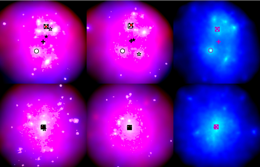
Figure 1: Examples of one visually and dynamically disturbed (upper panel) and one undisturbed (lower panel) galaxy cluster at $z=0$ from our suite of simulations (AGN, CSF, DM, from left to right). For the hydrodynamical simulated clusters, we use blue and red colours to represent dark matter and gas particle (SPH) densities, white represents optical stellar luminosity with a surface brightness of $\mu\geq 26.5~{}mag/arcsec^{2}$ in the SDSS r band; the DM only equivalent is shown in the rightmost panel. The symbols (+,x,$\circ$,$\square$) identify the location of the cluster centre of mass (+); minimum of the gravitational potential (x); maximum of SPH kernel weighted density ($\circ$); and the iterative centre of mass ($\square$). For the two hydrodynamical runs, we show also the BCG position in SDSS $r$ band using red filled circles. The open and filled black star symbols indicate the X-ray peak and centroid positions, respectively. We refer to section §3 for more details of these centre definitions.

We use three large–volume cosmological simulations, namely two hydrodynamical simulations in which we include different feedback processes, and one dark matter only N-body simulation. All these simulations are described in Cui et al. (2012); Cui et al. (2014b); here we summarise the relevant details.

We assume a flat $\Lambda$CDM cosmology, with cosmological parameters of $\Omega_{\rm m}=0.24$ for the matter density parameter, $\Omega_{\rm b}=0.0413$ for the baryon contribution, $\sigma_{8}=0.8$ for the power spectrum normalisation, $n_{\rm s}=0.96$ for the primordial spectral index, and $h=0.73$ for the Hubble parameter in units of $100~{}h~{}{\rm km}~{}s^{-1}~{}{\rm Mpc}^{-1}$. The three simulations were set up using the same realisation of the initial matter power spectrum, and reproduce the same large-scale structures. We refer to the dark matter only simulation as the DM run. Both hydrodynamical simulations include radiative cooling, star formation and kinetic feedback from supernovae; in one case we ignore feedback from AGN (which is referred as the CSF run), while in the other we include it (which is referred as the AGN run).

We use the TreePM-SPH code GADGET-3, an improved version of the public GADGET-2 code (Springel, 2005), which includes a range of prescriptions for galaxy formation physics (e.g. cooling, star formation, feedback). Gravitational forces are computed using a Plummer equivalent softening fixed to $\epsilon_{Pl}=7.5~{}h^{-1}~{}{\rm kpc}$ from z = 0 to 2 and fixed in comoving units at a higher redshift. As we will see, our softening length $7.5~{}h^{-1}~{}{\rm kpc}$ is comparable to – and in cases larger than – the offsets between the minimum potential and maximum SPH density positions, centre of BCGs and X-ray emission-weighted centres. However, the minimum potential position is determined by the whole cluster, which should be less affected by the softening length. Thus, we expect that these offsets are accurate to within a softening length.

Haloes are identified using the spherical overdensity (SO) algorithm PIAO (Cui et al., 2014b), assuming an overdensity criterion of $\Delta_{c}=200$ . Densities are computed using a SPH kernel smoothed over the nearest 128 neighbours; this allows us to determine the maximum density in the halo, which we also identify as the density-weighted centre of the halo. All of the particle types (dark matter, gas, stars) contribute equally to the density computation.

We select our cluster sample from the DM run SO halo catalogue, with the requirement that $M_{200}>2.0\times 10^{14}~{}h^{-1}\>{\rm M_{\odot}}$; this gives a total of 184 halos in our sample, with a maximum mass of $\sim 1.2\times 10^{15}~{}h^{-1}\>{\rm M_{\odot}}$. The corresponding SO halos in the AGN and CSF runs are identified by cross-matching the dark matter components using the unique particle IDs (see more details in Cui et al., 2014b); we find no systems less massive than $1.7\times 10^{14}~{}h^{-1}\>{\rm M_{\odot}}$ in this cross-matched catalogue. In this paper, we only focus on the clusters at redshift $z=0$.

Examples of a visually and dynamically disturbed and undisturbed clusters (lower and upper panels respectively) at $z=0$ are shown in Fig. 1, where we show qualitative projected density distributions in the AGN, CSF and DM runs (from left to right). In the case of the dark matter maps (rightmost panels), only the dark matter contributes to the RGB value of a pixel. The projected density of dark matter within a pixel lies in the range (0,255), and this is used to set the “B” of the RGB value of the pixel; if this density exceeds a threshold, we set the RGB value to white. When combining dark matter, gas and stars (leftmost and middle panels), both the dark matter and gas contribute to the RGB value. As before, the projected density of dark matter is scaled to the range (0,255), but without a threshold, and it is used to set the “B” of the RGB value; the projected density of has is scaled to the range (0,255) and is used to set the “R” of the RGB value; and the RGB value of stars is set to white, with a transparency of 0.5. By constructing the projected density maps in this way, we can get a sense for the relative projected densities of dark matter and gas in the systems; the projected dark matter density dominates the hot gas density at larger radii in both systems, but is dominated by the hot gas density at smaller radii.

3 The cluster centre identification

In this paper, we focus on 4 different definitions of the cluster centre. We quote centres of potential and density, which are readily measured in the simulation data, by their 3D values, while we use projected (2D) values for centres derived from mock observational data.

Minimum of the Gravitational Potential:

This is the physically intuitive definition of the cluster centre, and is expected to correspond to the lensing centre. For all particles within the $r_{200}$ radius, we select the one with the most negative value of the potential as the cluster centre. The particle’s potential is directly coming from the simulations. We will take this minimum potential position as the base line for comparison in this paper.

Maximum of the SPH Density:

In constructing our halo catalogue using the SO algorithm implemented in PIAO, we estimate the densities of particles by smoothing over nearest neighbours using the SPH kernel, and identify the particle with the highest density as the halo centre.

Optical Centres of the BCG:

Our hydrodynamical CSF and AGN runs include star formation. Using the method applied in Cui et al. (2011), we assign luminosities to each of the star particles that form by assuming that they constitute single stellar populations with ages, metallicities and masses given the corresponding particle’s properties in the run. Adopting the same initial mass function as the simulation, the spectral energy distribution of each particle is computed by interpolating the simple stellar population templates of Bruzual & Charlot (2003). We consider the three standard SDSS $r$, $g$, and $u$ bands in this paper. The luminosity of each star particle is smoothed to a 2-D map (projected to the xy-plane), with each pixel having a size of $5~{}h^{-1}~{}{\rm kpc}$. We adopt the same spline kernel used for the SPH calculations with 49 SPH neighbours, which is equivalent to $30~{}h^{-1}~{}{\rm kpc}$ (see Cui et al., 2014a, for more details). Note that the minimum offset cut for later relevant plots will be set to half the image pixel size, $2.5~{}h^{-1}~{}{\rm kpc}$.

The centre of BCG is identified as the most luminous image pixel of each band within the BCG. To select the BCG, we first separate the intra-cluster light from galaxies. As shown in Fig. 1, the surface brightness cut ($\mu\geq 26.5~{}mag/arcsec^{2}$) employed observationally is not suitable for our simulated data because it would include too much intra-cluster light. Cui et al. (2014a) has shown that the physical intra-cluster light identification method (based on the star’s velocity information Dolag et al., 2010) implies much higher surface brightness threshold values. For this reason, we adopt the surface brightness threshold values, $\mu=23,24.75~{}mag/arcsec^{2}$ for the CSF and AGN runs, respectively. Although these two values are for V-band luminosity in Cui et al. (2014a), we apply them here to the three SDSS bands without further corrections. This is because we are only interested in position of the brightest pixel inside the BCG in this paper; corrections should not affect our final results. Pixels above the surface brightness threshold are grouped together to form a galaxy by linking all neighbouring pixels, starting from the brightest pixel. The most luminous galaxy is selected as the BCG. In each band, we select the centre of the most luminous pixel inside the BCG as the centre.

Centres of X-ray Emission:

We estimate the X-ray emission from each of the simulated clusters using the PHOX code (see Biffi et al., 2012; Biffi et al., 2013, for a more detailed description). Specifically, we simulate the X-ray emission of the intra-cluster medium (ICM) by adopting an absorbed APEC model Smith et al. (2001), where the WABS absorption model Morrison & McCammon (1983) is used to mimic the Galactic absorption and the main contribution from the hot ICM comes in the form of bremsstrahlung continuum plus metal emission lines. The latter is obtained from the implementation of the APEC model for a collisionally-ionized plasma comprised within the XSPEC package (v.12.8.0). For any gas element in the simulation output, the model spectrum predicts the expected number of photons, with which we statistically sample the spectral energy distribution.

In the approach followed by PHOX, the synthetic X-ray photons are obtained from the ideal emission spectrum calculated for every gas particle belonging to the cluster ICM, depending on its density, temperature, metallicity and redshift (we assume $z=0.05$ for the X-ray luminosity and angular-diameter distances). We consider only the position of the X-ray centre in this work, and do not expect the particular choice of redshift or metallicity to affect it significantly. To obtain the photon maps, we assume a realistic exposure time of 50 ks and convolve the ideal photon-list of every cluster with the response matrices of Chandra (ACIS-S detector); this accounts for the instrument characteristics and sensitivity to the incoming photon energies. In this process, the maps (i) are originally centered on the cluster potential centre, (ii) cover a circular region of $R_{200}$ radius, and (iii) have a the same pixel size of $5~{}h^{-1}~{}{\rm kpc}$ as the optical image.

In this work, we consider the $x$-$y$ projection and the full energy band of the detector. In addition, we also apply the same SPH smoothing procedure as used for the optical image, but using each pixel’s photon counts from the PHOX X-ray maps instead of stellar luminosity. The X-ray peak position is identified as the pixel with the maximum value of photon counts. We note here that using this simple X-ray peak position as the X-ray centre can be biased by the satellites (see Mantz et al., 2015, for more discussions about different X-ray centre tracers). The centroid of the X-ray map is computed basing on the method of Böhringer et al. (2010); Rasia et al. (2013), modified to take the X-ray peak position as the initial centre and reset to the centre of mass from photon counts within the shrinking radius after each iteration. We reduce the radius to $85$ per cent of the previous iteration, starting at an initial radius of $R_{200}$ in projection, until a fixed inner radius $R_{2500}$ is reached. The X-ray centroid is the centre of mass position at the final step. We use this iterative method to locate the centroid, because there are many un-relaxed clusters in our sample. Note that the minimum offset cut for later relevant plots is also set to the size of half a pixel, $2.5~{}h^{-1}~{}{\rm kpc}$.

4 Results

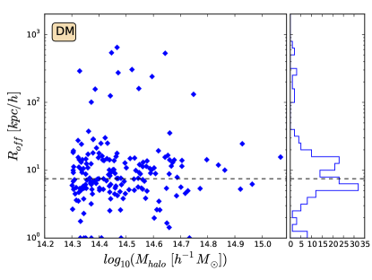
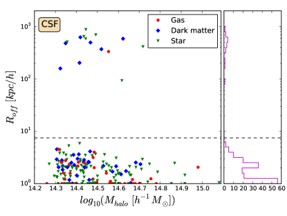
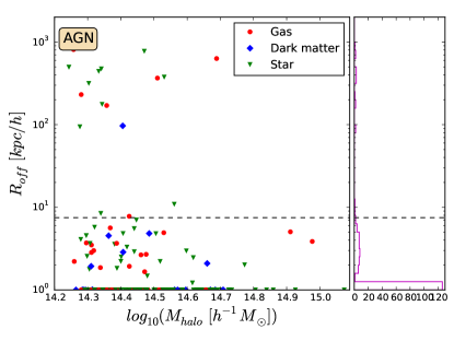
Figure 2: The offset between the maximum SPH density and minimum potential positions as a function of halo mass. From top to bottom, these panels are for DM, CSF, AGN runs, respectively; On the right hand of each panel, we show a histogram distribution of the offsets. The horizontal dashed lines are the softening length in the simulations. As indicated in the legends of middle and bottom panels, the different color symbols represent the type of the highest density particle, i.e. cluster centre.

4.1 Offsets between maximum SPH density and minimum potential positions

	Gas	Dark matter	Star
CSF	36	38	110
AGN	50	18	116

Table 1: Numbers of clusters in which the densest particle belongs to a given particle type (i.e. gas, dark matter or stars).

In Fig. 2, we investigate the offset between the maximum of SPH density and the minimum of the gravitational potential positions in the DM, CSF and AGN runs (upper, middle and lower panels respectively). We reset offsets $R_{off}<1~{}h^{-1}~{}{\rm kpc}$ to $1~{}h^{-1}~{}{\rm kpc}$, for an easier visualization.

• In the DM run, we find typical offsets of $\sim 10~{}h^{-1}~{}{\rm kpc}$, which is comparable with the simulation softening length as indicated by the horizontal dashed line in all panels. Those clusters with large offsets contain massive compact substructures that are in the process of merging and the system shows obvious signs of disturbance.

• In the CSF run, the typical offsets are smaller than the softening length of the simulation ($\lower 2.15277pt\hbox{$\;\buildrel<\over{\sim}\;$}3~{}h^{-1}~{}{\rm kpc}$), but in some cases there are offsets as large as $\lower 2.15277pt\hbox{$\;\buildrel>\over{\sim}\;$}100~{}h^{-1}~{}{\rm kpc}$. Close inspection shows that star and dark matter particles tend to be the particles defining the maximum SPH density within these systems; we indicate this explicitly by marking the particles that trace the maximum of the density with symbols defined in the legend.

• In common with the CSF run, the majority of clusters in the AGN run have offsets smaller than the softening length, $\lower 2.15277pt\hbox{$\;\buildrel<\over{\sim}\;$}1~{}h^{-1}~{}{\rm kpc}$. As in the CSF run, and as shown in table 1, star particles tend to define the location of the density peak.

We have visually inspected those clusters that have large offsets in Fig. 2 and find, unsurprisingly, that the density peak is associated with a massive satellite galaxy (e.g. the disturbed cluster in the upper row of Fig. 1). This indicates that these clusters with large offsets are normally undergoing major mergers and are visually disturbed.

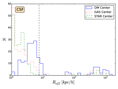
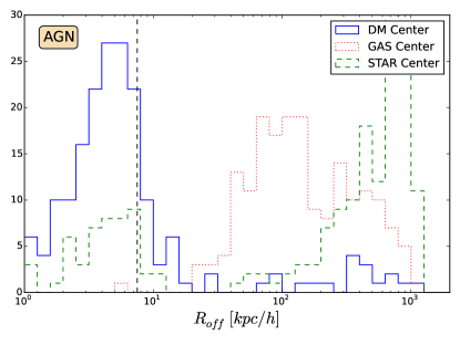
Figure 3: As in Fig. 2, we show the offset between the density and potential centres in the CSF (left panel) and AGN (right panel) runs, but now we split according to particle type, where solid, dotted and dashed histograms correspond to dark matter, gas and stars respectively. Note that offsets $R_{off}<1~{}h^{-1}~{}{\rm kpc}$ are reset to $1~{}h^{-1}~{}{\rm kpc}$.

We did not differentiate between the material that contributes to the estimate of the maximum SPH density position (i.e. gas, star and dark matter particles are given equal weight) in Fig. 2; we now show this in Fig. 3. Here the maximum SPH density positions computed from each of the three particle types are offset with respect to the potential centre of the cluster in the CSF and AGN runs (left and right panels respectively). In this calculation, we include only particles of the same species (i.e. dark matter, gas, stars) when calculating densities. The particle with the maximum SPH density is selected as the density peak for the given component.

In the CSF run, there is broad agreement between the maximum SPH density and minimum potential position offsets computed for each of the particle types; these offsets are within $\sim 10~{}h^{-1}~{}{\rm kpc}$, while those systems with offsets $\gtrsim 300~{}h^{-1}~{}{\rm kpc}$ are visually idenitified as disturbed. In stark contrast to the CSF run and also to the result from Fig. 2, in the AGN run there is a clear separation in the maximum SPH density and minimu potential position offsets computed from dark matter particles on the one hand and star and gas particles on the other. The dark matter particles have offsets similar to those found in the CSF run, clustering within $\sim 10~{}h^{-1}~{}{\rm kpc}$, but the star particles have two offset peaks at $\sim 7$ and $\sim 900~{}h^{-1}~{}{\rm kpc}$, while gas particles particles have offsets spread between $\sim 50-800~{}h^{-1}~{}{\rm kpc}$. The large offsets we see in the stellar component arise because the identified centres are located in satellite galaxies, which are compact, rather than in the BCG. This is also linked to the large offsets we find in the gas component, which arise because strong AGN feedback can expel gas to a large cluster-centric radius and helps to suppress star formation over much of the lifetime of the BCG by inhibiting the accumulation of dense gas at small radii. Similar trends arising from AGN have been reported in Ragone-Figueroa et al. (2012, 2013); Cui et al. (2014a). Note that this figure is primarily of theoretical interest; it shows how the centre of density changes as we sample the different components in the simulation, something that would be challenging to do observationally!

4.2 Offsets between BCG and potential centres

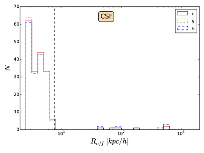
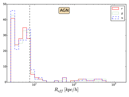
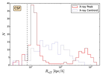
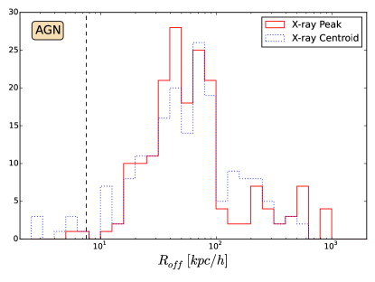
Figure 4: The histogram of the offsets between centre of BCGs and cluster potential centre. Left panel is the results from CSF clusters, while the right panel is for AGN clusters. Three optical luminosity bands $u$, $g$, $r$ are indicated in the upper-right legend. The vertical dashed lines are the softening length in the simulations.

Figure 5: Similar to Fig. 5, the histogram of the offsets between X-ray centres and the cluster potential centre. Left panel is the results from CSF clusters, while the right panel is for AGN clusters. The peak and centroid indicators are shown in the legend. The vertical dashed lines are the softening length in the simulations.

We now consider the relationship between the centre of BCGs and minimum potential positions, where we employ the method of Cui et al. (2011) as described in § 3 to assign luminosity to star particles in the SDSS $u$, $g$ and $r$ bands. Note that we do not include the effects of dust when calculating luminosities, and so we potentially omit band-dependent dust attenuation that could, in principle, bias our conclusion. To compare with observations, we focus on 2D $x$-$y$ projections here. The minimum offset is set to half of the pixel size $2.5~{}h^{-1}~{}{\rm kpc}$.

In Fig. 5 we show how the distribution of offsets between the centre of BCGs and minimum potential positions. The results for both the CSF and AGN runs (left and right panels respectively) are in broad agreement, and similar to those shown in Fig. 2 for the offset between density and potential peaks; most of the offsets are within the softening length for both CSF and AGN runs. We find no dependence on measured (i.e. $u$, $g$ or $r$) band.

4.3 Offsets between X-ray and potential centres

In Fig. 5, we show the distribution of offsets between the X-ray peak, centroid positions and cluster potential centre in the CSF and AGN runs (left and right panels respectively). Here we note some interesting differences.

• In the CSF run, the offset distributions of peak positions show a peak at $\sim 10~{}h^{-1}~{}{\rm kpc}$, with a second peak at $\sim 700~{}h^{-1}~{}{\rm kpc}$; this is larger than for the offset between the centre of BCGs and minimum potential positions. While, the X-ray centroid offset show a wide spread distribution from $\sim 10~{}h^{-1}~{}{\rm kpc}$ towards $\sim 200~{}h^{-1}~{}{\rm kpc}$.

• In the AGN run, the offset distributions for both X-ray peak and centroid have a peak at $\sim 50~{}h^{-1}~{}{\rm kpc}$. This is slightly less than the offsets between the gas component density and cluster potential centres from Fig. 3.

Compared with the X-ray peak centre, the centroid is more stable for both CSF and AGN runs. They tend to have similar distributions, despite the AGN feedback model. However, the centroid offsets from CSF runs have no clear peak compared to the AGN runs. There is no strong evidence of the secondary peak for the centroid offsets. The X-ray peak offsets for CSF run are smaller than the AGN run, which indicates that the AGN feedback has stronger effects on the X-ray peak position.

These results suggest that the centre of BCGs should be a more reliable and precise tracer of the underlying gravitational potential, and is also less likely to be influenced by the AGN feedback.

5 Discussion and Conclusions

Using a suite of cosmological $N$-body and hydrodynamical simulations, we have constructed a mass- and volume-complete simulated galaxy cluster catalogue. We have considered a pure dark matter (i.e. $N$-body only) model and two galaxy formation models that include cooling, star formation and supernova feedback, with and without AGN feedback (the CSF and AGN runs respectively); this allows us to explore in a systematic fashion the impact of these two baryon models on the properties of galaxy clusters. In this paper, we have assessed how estimates of galaxy cluster centres are influenced by the mode of measurement – using X-ray emitting hot gas, the centre of BCGs, or the total mass distribution, which is accessible via gravitational lensing, say. In all cases we compare to the location of the minimum of the gravitational potential of the system, which we would expect to define a physically reasonable centre of the system, assuming that it is in dynamical equilibrium.

The main results of our analysis are summarised as follows.

• We find that the maximum local density, computed using an SPH kernel smoothing over 128 nearest neighbours, is in good agreement with the minimum of the gravitational potential regardless of the assumed galaxy formation model, provided we include all particles – dark matter, gas and stars – in the calculation. In the CSF runs, we find offsets between the maximum SPH density and minimum potential positions at $\lower 2.15277pt\hbox{$\;\buildrel<\over{\sim}\;$}3~{}h^{-1}~{}{\rm kpc}$; in the AGN runs, these offsets are even smaller than the CSF runs. However, both runs have a small amount of clusters with very large offsets ($\lower 2.15277pt\hbox{$\;\buildrel>\over{\sim}\;$}100~{}h^{-1}~{}{\rm kpc}$). This is because the density peak is associated with a satellite galaxy.

  If we compute the maximum local density for individual particle types, we find differences that depend on the assumed galaxy formation model. The offsets for different particles in CSF run are within the simulation softening length. However, many clusters in AGN run have very large offsets between the density peak evaluated from both stellar and gas particles and the potential centre. The strong feedback from the AGN not only expels gas particles, which have the offset at $\sim 100~{}h^{-1}~{}{\rm kpc}$, but also reduces the stellar density within the central galaxy, in which case the peak of the stellar density is more likely to be associated with a satellite galaxy.

• Using projected optical luminosities in SDSS $r$, $g$ and $u$ bands, we identify the centre of BCG from star particles in the CSF and AGN runs. We find that centre of BCGs are close to the potential centre, within the softening length in both runs and independent of the assumed band. A small fraction of the clusters have large offsets in both CSF and AGN runs; these belong to disturbed clusters, in which the identified BCG is offset from the centre of the potential by visually checking.

• Identifying the location of both the peak and centroid positions of X-ray emission from realistic maps, we find slightly larger peak offsets $\sim 10~{}h^{-1}~{}{\rm kpc}$ in the CSF run (with a second peak at $\sim 700~{}h^{-1}~{}{\rm kpc}$); $\sim 50~{}h^{-1}~{}{\rm kpc}$ in the AGN run. The X-ray centroid offset seem more stable than X-ray peak, which have less effect from the AGN feedback. It has a wide spread from $\sim 10~{}h^{-1}~{}{\rm kpc}$ to $\sim 200~{}h^{-1}~{}{\rm kpc}$. There is no clear peak in the CSF run; while the AGN run has a similar peak as its X-ray peak offset.

It is interesting to ask how well our simulations match observations, which has a bearing on the general applicability of our results. We note that we have already used the same cosmological simulation data to compare baryon and stellar mass fractions with observations in Cui et al. (2014b) (see their Fig. B1 for details). There it was shown that both of these fractions computed from our AGN simulation are consistent with observations, whereas the CSF runs predict values that are larger than observed; this is to be expected, arising because of overcooling. In the nIFTy cluster comparison project Sembolini et al. 2015a, b, a single galaxy cluster has been simulated in a cosmological context with a range of state-of-the-art astrophysics codes, and in the runs that employ the physics of galaxy formation (e.g. radiative cooling, star formation, feedback from supernovae and AGN) it has been shown the results from the model used in this paper is consistent with the results of other codes (Sembolini et al. 2015b; Cui et al., In Preparation) in global cluster properties. However, galaxies inside this cluster show striking code-to-code variations in stellar and gas mass (Elahi et al., 2015), which implies different spatial distributions for the gas and stellar components. Thus, we caution that the choice of input physics in simulations of this kind can have a strong quantitative influence on the results.

We find that the distribution of offsets between the centre of BCG and X-ray emission centres with respect to the potential centre is smaller than is found observationally; this could be due to in part to observational inaccuracies (image resolution, identification of lensing centre) and in part to our assumption that the potential centre, calculated from the 3D distribution of matter within the cluster, is well-matched to the lensing centre. However, our results agree with observations that centre of BCG is a better tracer of the cluster centre than the X-ray emission weighted centre (George et al., 2012). However, the claim that the BCG is a better tracer requires identifying BCGs correctly in the first place in observations, which is not straightforward. Our simulation results suggest that the simple grouping method after ICL extraction in Section 3 does a good job. Offsets between X-ray and lensing centres are in fact observed at a level of 100 kpc (e.g. Allen, 1998; Shan et al., 2010a; George et al., 2012). However, the observed offsets between lensing and BCGs are usually smaller. For example, Oguri et al. (2010) found that the offsets between weak lensing and BCG are at $\sim 50~{}h^{-1}~{}{\rm kpc}$, while the strong lensing has even closer position to BCG (Oguri et al., 2009). With large statistical samples, Zitrin et al. (2012) also suggested smaller offsets between the weak lensing and BCG position. These support that the BCG traces the minimum gravitational potential position better than the X-ray data.

The large offset tail found in clusters from both the centre of BCG and X-ray center are basically consistent with the secondary peak found by Johnston et al. (2007); Zitrin et al. (2012). These large offsets should be caused by dynamically unrelaxed clusters undergoing mergers, in which the optical luminosity and X-ray centres can be located at a massive satellite galaxy, which is away from the cluster potential centre. Using a set of hydrodynamical simulations of mergers of two galaxy clusters, Zhang et al. (2014) find that significantly large SZ-X-ray peak offsets (>100 kpc) can be produced during the major mergers of galaxy clusters. This finding is basically agreed to the second peak for X-ray peak-potential offsets from our CSF runs. These large offsets indicate these clusters are not relaxed. This highlights the importance of dynamical state in the centre determination, something we will address in a follow-up paper.

Finally, we have considered only spatial offsets in this study, the first of a series. We expect to find dynamical offsets within clusters. Subhaloes or satellite galaxies in N-body and hydrodynamic simulations are found to have velocities differing from the dark matter halos (e.g. Diemand et al., 2004; Gao et al., 2004; Gill et al., 2004b; Munari et al., 2013; Wu et al., 2013). These velocity offsets are closely connected to the cluster center offsets. Gao & White (2006); Behroozi et al. (2013) demonstrated that dark matter halo cores are not at rest relative to the halo bulk or substructure average velocities and have coherent velocity offsets across a wide range of halo masses and redshifts. We revisit this using our cluster sample in our next paper, surveying not only the dark matter but also gas and stars, and consider its implications for turbulence and accretion onto AGN.

Appendix A Identifying Density Peaks

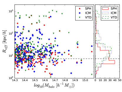
Figure 6: The offsets between three density peak estimators – SPH, Voronoi tessellation density (VTD), and the iterative centre of mass (ICM) – and the location of the minimum of the gravitational potential, as a function of cluster mass. Red circles, blue diamonds and green inverted triangles correspond to SPH, ICM and VTD estimators respectively. The right panel shows the histograms of the offsets. See text for further details.

We considered a number of approaches to estimating the location of the maximum density of the cluster. Here we briefly review three – one that was used in the study, and two others from the literature.

• The Smoothed Particle Hydrodynamics (SPH) method adopts the kernel smoothing approach that is commonly used in hydrodynamics; we have implemented and tested this method in Cui et al. (2014b) using 128 neighbours when calculating densities. This is the method used in the PIAO halo finder and the one used in this study.

• The Iterative Centre of Mass (ICM) method estimates the mass-weighted centre in an iterative fashion, using all particles within a shrinking spherical volume until convergence in the estimated centre is achieved (cf. Power et al., 2003); we define convergence when consecutive centres agree to within $1~{}h^{-1}~{}{\rm kpc}$.

• The Voronoi Tessellation Density (VTD) method partitions the volume into cells using the distance between adjacent points to define cell boundaries, and uses the inverse volume of the cell to estimate the local density at the position of each particle; it requires no free parameters. We use the publicly available convex hulls program (Clarkson, 1992) implemented in python. We note that this approach is sensitive to the finite resolution of the simulation.

In Fig. 6, we show the offsets between the three estimates (SPH, ICM, and VTD) of the maximum density position and the location of the minimum of the gravitational potential (red circles, blue diamonds and green inverted triangles, respectively) for each of the clusters in our DM sample. The histograms in the right hand panel are the corresponding to projected distributions of cluster offsets. Fig. 6 shows that the performance of the three estimators, as measured by the typical size of offset with respect to the location of the minimum of the gravitational potential, is comparable, although the SPH method – implemented in PIAO and used in this study – should be favoured – $87.5$ per cent of the total offsets are within $20~{}h^{-1}~{}{\rm kpc}$.

References

- Allen (1998) Allen S. W., 1998, MNRAS, 296, 392
- Anders & Grevesse (1989) Anders E., Grevesse N., 1989, Geochim. Cosmochim. Acta, 53, 197
- Behroozi et al. (2013) Behroozi P. S., Wechsler R. H., Wu H.-Y., 2013, ApJ, 762, 109
- Biffi et al. (2012) Biffi V., Dolag K., Böhringer H., Lemson G., 2012, MNRAS, 420, 3545
- Biffi et al. (2013) Biffi V., Dolag K., Böhringer H., 2013, MNRAS, 428, 1395
- Böhringer et al. (2004) Böhringer H., et al., 2004, A&A, 425, 367
- Böhringer et al. (2010) Böhringer H., et al., 2010, A&A, 514, A32
- Bruzual & Charlot (2003) Bruzual G., Charlot S., 2003, MNRAS, 344, 1000
- Clarkson (1992) Clarkson K. L., 1992, in Proc. 31st IEEE Symposium on Foundations of Computer Science. Pittsburgh, PA, pp 387–395, http://cm.bell-labs.com/who/clarkson/dets.html
- Cui et al. (2011) Cui W., Springel V., Yang X., De Lucia G., Borgani S., 2011, MNRAS, 416, 2997
- Cui et al. (2012) Cui W., Borgani S., Dolag K., Murante G., Tornatore L., 2012, MNRAS, 423, 2279
- Cui et al. (2014a) Cui W., et al., 2014a, MNRAS, 437, 816
- Cui et al. (2014b) Cui W., Borgani S., Murante G., 2014b, MNRAS, 441, 1769
- Davis et al. (1985) Davis M., Efstathiou G., Frenk C. S., White S. D. M., 1985, ApJ, 292, 371
- De Lucia et al. (2004) De Lucia G., Kauffmann G., Springel V., White S. D. M., Lanzoni B., Stoehr F., Tormen G., Yoshida N., 2004, MNRAS, 348, 333
- Diemand et al. (2004) Diemand J., Moore B., Stadel J., 2004, MNRAS, 352, 535
- Dolag et al. (2009) Dolag K., Borgani S., Murante G., Springel V., 2009, MNRAS, 399, 497
- Dolag et al. (2010) Dolag K., Murante G., Borgani S., 2010, MNRAS, 405, 1544
- Du & Fan (2014) Du W., Fan Z., 2014, ApJ, 785, 57
- Ebeling et al. (1998) Ebeling H., Edge A. C., Bohringer H., Allen S. W., Crawford C. S., Fabian A. C., Voges W., Huchra J. P., 1998, MNRAS, 301, 881
- Elahi et al. (2015) Elahi P. J., et al., 2015, preprint, (arXiv:1511.08255)
- Forero-Romero et al. (2010) Forero-Romero J. E., Gottlöber S., Yepes G., 2010, ApJ, 725, 598
- Gao & White (2006) Gao L., White S. D. M., 2006, MNRAS, 373, 65
- Gao et al. (2004) Gao L., White S. D. M., Jenkins A., Stoehr F., Springel V., 2004, MNRAS, 355, 819
- George et al. (2012) George M. R., et al., 2012, ApJ, 757, 2
- Gill et al. (2004a) Gill S. P. D., Knebe A., Gibson B. K., 2004a, MNRAS, 351, 399
- Gill et al. (2004b) Gill S. P. D., Knebe A., Gibson B. K., Dopita M. A., 2004b, MNRAS, 351, 410
- Gladders & Yee (2000) Gladders M. D., Yee H. K. C., 2000, AJ, 120, 2148
- Guo et al. (2015) Guo H., et al., 2015, MNRAS, 446, 578
- Hunter (2007) Hunter J. D., 2007, Computing In Science & Engineering, 9, 90
- Johnston et al. (2007) Johnston D. E., Sheldon E. S., Tasitsiomi A., Frieman J. A., Wechsler R. H., McKay T. A., 2007, ApJ, 656, 27
- Knebe et al. (2011) Knebe A., Knollmann S. R., Muldrew S. I., et al., 2011, MNRAS, 415, 2293
- Knebe et al. (2013) Knebe A., Pearce F. R., Lux H., Ascasibar Y., et al., 2013, MNRAS,
- Knollmann & Knebe (2009) Knollmann S. R., Knebe A., 2009, ApJS, 182, 608
- Koester et al. (2007) Koester B. P., et al., 2007, ApJ, 660, 221
- Kravtsov & Borgani (2012) Kravtsov A. V., Borgani S., 2012, ARA&A, 50, 353
- Lacey & Cole (1994) Lacey C., Cole S., 1994, MNRAS, 271, 676
- Lin & Mohr (2004) Lin Y.-T., Mohr J. J., 2004, ApJ, 617, 879
- Liu et al. (2013) Liu T., Tozzi P., Tundo E., Moretti A., Wang J.-X., Rosati P., Guglielmetti F., 2013, A&A, 549, A143
- Mandelbaum et al. (2008) Mandelbaum R., Seljak U., Hirata C. M., 2008, JCAP, 8, 6
- Mann & Ebeling (2012) Mann A. W., Ebeling H., 2012, MNRAS, 420, 2120
- Mantz et al. (2015) Mantz A. B., Allen S. W., Morris R. G., Schmidt R. W., von der Linden A., Urban O., 2015, MNRAS, 449, 199
- Mohr et al. (1993) Mohr J. J., Fabricant D. G., Geller M. J., 1993, ApJ, 413, 492
- Morrison & McCammon (1983) Morrison R., McCammon D., 1983, ApJ, 270, 119
- Munari et al. (2013) Munari E., Biviano A., Borgani S., Murante G., Fabjan D., 2013, MNRAS, 430, 2638
- Oguri et al. (2009) Oguri M., et al., 2009, ApJ, 699, 1038
- Oguri et al. (2010) Oguri M., Takada M., Okabe N., Smith G. P., 2010, MNRAS, 405, 2215
- Planck Collaboration et al. (2011) Planck Collaboration et al., 2011, A&A, 536, A8
- Poole et al. (2006) Poole G. B., Fardal M. A., Babul A., McCarthy I. G., Quinn T., Wadsley J., 2006, MNRAS, 373, 881
- Postman et al. (1996) Postman M., Lubin L. M., Gunn J. E., Oke J. B., Hoessel J. G., Schneider D. P., Christensen J. A., 1996, AJ, 111, 615
- Power et al. (2003) Power C., Navarro J. F., Jenkins A., Frenk C. S., White S. D. M., Springel V., Stadel J., Quinn T., 2003, MNRAS, 338, 14
- Power et al. (2012) Power C., Knebe A., Knollmann S. R., 2012, MNRAS, 419, 1576
- Ragone-Figueroa et al. (2012) Ragone-Figueroa C., Granato G. L., Abadi M. G., 2012, MNRAS, 423, 3243
- Ragone-Figueroa et al. (2013) Ragone-Figueroa C., Granato G. L., Murante G., Borgani S., Cui W., 2013, MNRAS, 436, 1750
- Ramella et al. (2001) Ramella M., Boschin W., Fadda D., Nonino M., 2001, A&A, 368, 776
- Rasia et al. (2013) Rasia E., Meneghetti M., Ettori S., 2013, The Astronomical Review, 8, 40
- Robotham et al. (2011) Robotham A. S. G., et al., 2011, MNRAS, 416, 2640
- Rozo & Rykoff (2014) Rozo E., Rykoff E. S., 2014, ApJ, 783, 80
- Sembolini et al. (2015a) Sembolini F., et al., 2015a, preprint, (arXiv:1503.06065)
- Sembolini et al. (2015b) Sembolini F., et al., 2015b, preprint, (arXiv:1511.03731)
- Shan et al. (2010a) Shan H., Qin B., Fort B., Tao C., Wu X.-P., Zhao H., 2010a, MNRAS, 406, 1134
- Shan et al. (2010b) Shan H. Y., Qin B., Zhao H. S., 2010b, MNRAS, 408, 1277
- Smith et al. (2001) Smith R. K., Brickhouse N. S., Liedahl D. A., Raymond J. C., 2001, ApJLett, 556, L91
- Springel (2005) Springel V., 2005, MNRAS, 364, 1105
- Springel et al. (2001) Springel V., White S. D. M., Tormen G., Kauffmann G., 2001, Monthly Notices of the Royal Astronomical Society, 328, 726
- Thomas et al. (1998) Thomas P. A., et al., 1998, MNRAS, 296, 1061
- Tinker et al. (2008) Tinker J., Kravtsov A. V., Klypin A., Abazajian K., Warren M., Yepes G., Gottlöber S., Holz D. E., 2008, ApJ, 688, 709
- Vanderlinde et al. (2010) Vanderlinde K., et al., 2010, ApJ, 722, 1180
- Williamson et al. (2011) Williamson R., et al., 2011, ApJ, 738, 139
- Wu et al. (2013) Wu H.-Y., Hahn O., Evrard A. E., Wechsler R. H., Dolag K., 2013, MNRAS, 436, 460
- Zhang et al. (2014) Zhang C., Yu Q., Lu Y., 2014, ApJ, 796, 138
- Zitrin et al. (2012) Zitrin A., Bartelmann M., Umetsu K., Oguri M., Broadhurst T., 2012, MNRAS, 426, 2944
- van den Bosch et al. (2005) van den Bosch F. C., Weinmann S. M., Yang X., Mo H. J., Li C., Jing Y. P., 2005, MNRAS, 361, 1203
- von der Linden et al. (2014) von der Linden A., et al., 2014, MNRAS, 439, 2