On freely floating bodies trapping
time-harmonic waves in water
covered by brash ice

Abstract

A mechanical system consisting of water covered by brash ice and a body freely floating near equilibrium is considered. The water occupies a half-space into which an infinitely long surface-piercing cylinder is immersed, thus allowing us to study two-dimensional modes of the coupled motion which is assumed to be of small amplitude. The corresponding linear setting for time-harmonic oscillations reduces to a spectral problem whose parameter is the frequency. A constant that characterises the brash ice divides the set of frequencies into two subsets and the results obtained for each of these subsets are essentially different.

For frequencies belonging to a finite interval adjacent to zero, the total energy of motion is finite and the equipartition of energy holds for the whole system. For every frequency from this interval, a family of motionless bodies trapping waves is constructed by virtue of the semi-inverse procedure. For sufficiently large frequencies outside of this interval, all solutions of finite energy are trivial.

1 Introduction

This paper continues the rigorous study (initiated in [3]) of a freely floating rigid bodies trapping time-harmonic waves in an inviscid, incompressible, heavy fluid, say water (see also [6, 7, 8] and [4]). We consider the infinitely deep water in irrotational motion bounded from above by a free surface unbounded in all horizontal directions, but unlike the cited papers dealing with the open surface, we assume here that it is totally covered with the brash ice. The body is supposed to be an infinitely long cylinder which allows us to consider two-dimensional modes orthogonal to cylinder’s generators. We also assume that the body is surface-piercing and unaffected by all external forces (for example due to constraints on its motion) except for gravity. The motion of the whole system is supposed to be of small amplitude near equilibrium, and so the linear model developed by John [2] is used to describe the coupled motion of water and body. However, the free-surface boundary condition must be amended to take into account the presence of the brash ice covering the water. Such a condition was proposed by Peters [10], who considered the brash ice as an infinitely thin mat whose particles do not interact; that is, the only forces acting on it are those due to gravity and the pressure of the water from below (see also [1]).

Our aim is twofold: first, we apply the so-called semi-inverse procedure for the construction of motionless two-dimensional bodies each trapping a time-harmonic mode; that is, the water covered by the brash ice and the body oscillate at the same frequency, whereas the energy of water and ice motion is finite. We recall that a trapped mode in two and three dimensions describes a free oscillation of the system that has finite energy (see [9], p. 17). This should be distinguished from edge waves and waves trapped around an array of cylinders.

It should be mentioned that the same semi-inverse procedure was used by Kuznetsov [3] for obtaining two-dimensional trapping bodies that are motionless in the open water (it is outlined in §4.1). However, there is an essential distinction between the case of the open water and the water covered by the brash ice. Namely, no restriction was imposed on the trapping frequencies in the former case. On the contrary, trapping frequencies are bounded by a constant characterising the brash ice and this bound is essential in the latter case. Indeed, our second result shows that if a solution of the problem has finite energy and the frequency exceeds a certain bound, then this solution is trivial. Generally, this bound is larger than the constant mentioned above, but these bounds may coincide for some bodies. It is essential that this result is valid for all bodies.

Figure 1: A definition sketch of the cylinder cross-section with immersed parts denoted by $B_{-}$ and $B_{+}$; their wetted boundaries are $S_{-}$ and $S_{+}$ respectively. The cross-section of the infinitely thin layer of the brash ice covering the free surface is denoted by $F$; it consists of three parts two of which lie on the $x$-axis outside $|x|>a$ and the third one is between $x=-b$ and $x=+b$; $W$ is the cross-section of the water domain.

2 Statement of the problem

Let the Cartesian coordinate system $(x,y)$ in a plane orthogonal to the generators of a freely floating infinitely long cylinder be chosen so that the $y$-axis is directed upwards, whereas the mean free surface of the water intersects this plane along the $x$-axis, and so the cross-section $W$ of the water domain is a subset of $\mathbb{R}^{2}_{-}=\{x\in\mathbb{R},\,y<0\}$. Let $\widehat{B}$ denote the bounded two-dimensional domain whose closure is the cross-section of a floating cylinder in its equilibrium position (see figure 1).

We suppose that $\widehat{B}\setminus\overline{\mathbb{R}^{2}_{-}}$ — the part of the body located above the surface of water covered by the brash ice — is a nonempty domain, whereas the immersed part $B=\widehat{B}\cap\mathbb{R}^{2}_{-}$ is the union of a finite number of domains (in particular, it may be a single domain). Thus, $D=\widehat{B}\cap\partial\mathbb{R}^{2}_{-}$ consists of the same number of nonempty intervals of the $x$-axis; see figure 1, where $D=\{x\in(-a,-b)\cup(b,a),\,y=0\}$ in the case of two immersed parts. We suppose that $W$ is $\mathbb{R}^{2}_{-}\setminus{\overline{B\mkern 2.0mu}\mkern-2.0mu}{}$. Furthermore, we assume that $W$ is a Lipschitz domain, and so the unit normal $\bm{n}$ pointing to the exterior of $W$ is defined almost everywhere on $\partial W$. Finally, we denote by $S=\partial\widehat{B}\cap\mathbb{R}^{2}_{-}$ the wetted curve (the number of its components is equal to the number of immersed domains), whereas $F=\partial\mathbb{R}^{2}_{-}\setminus{\overline{D\mkern 2.0mu}\mkern-2.0mu}{}$ is the infinitely thin layer of the brash ice covering the free surface at rest.

To describe the small-amplitude coupled motion of the system it is standard to apply the linear setting, in which case the first-order unknowns are used. These are the velocity potential $\mathop{\Phi\vrule height=1.93747pt,width=0.0pt}\nolimits(x,y;t)$ and the vector column $\mathop{\bm{q}\vrule height=1.93747pt,width=0.0pt}\nolimits(t)$ describing the motion of the body. This vector has the following three components:

$\bullet$ $q_{1}$ and $q_{2}$ are the displacements of the centre of mass in the horizontal and vertical directions respectively from its rest position $\bigl{(}x^{(0)},y^{(0)}\bigr{)}$;

$\bullet$ $q_{3}$ is the angle of rotation about the axis that goes through the centre of mass orthogonally to the $(x,y)$-plane (the angle is measured from the $x$- to the $y$-axis).

On the surface $F$, the brash ice is characterised by a non-negative function $\sigma$ equal to the ratio of the local area density of the brash ice to the constant volume density of the water. The values of $\sigma$ are less than or equal to one, and we assume that $\sigma$ is constant throughout $F$; the value of this constant is defined by the water salinity.

We omit relations governing the general time-dependent motion (see the details in [3]) and turn directly to the time-harmonic oscillations of the system for which purpose we use the ansatz

$$\bigl{(}\mathop{\Phi\vrule height=1.93747pt,width=0.0pt}\nolimits(\bm{x},y,t),\bm{q}(t)\bigr{)}={\rm Re}\bigl{\{}\textrm{e}^{-\kern 0.35002pt\mathrm{i}\kern 0.35002pt\omega t}\bigl{(}\mathop{\varphi\vrule height=1.93747pt,width=0.0pt}\nolimits(\bm{x},y),\kern 0.50003pt\mathrm{i}\kern 0.50003pt\bm{\chi}\bigr{)}\bigr{\}},$$ (1)

where $\omega>0$ is the radian frequency, $\varphi\in\mathop{H^{1}_{loc}\vrule height=1.93747pt,width=0.0pt}\nolimits(W)$ is a complex-valued function bounded at infinity and $\bm{\chi}\in\varmathbb{C}^{3}$. Then the governing relations for $\bigl{(}\varphi,\bm{\chi}\bigr{)}$ are as follows:

$$\nabla^{2}\varphi=0\quad\mbox{in}\ W;$$ (2)

$$\mathchoice{\raise-0.5pt\hbox{$\partial$}\vphantom{\partial}_{\mkern-1.5muy}^{\mkern 0.4mu}\mkern 0.3mu}{\raise-0.5pt\hbox{$\partial$}\vphantom{\partial}_{\mkern-1.5muy}^{\mkern 0.4mu}\mkern 0.3mu}{\raise-0.5pt\hbox{$\scriptstyle\partial$}\vphantom{\partial}_{\mkern-1.7muy}\mkern 0.1mu}{\raise-0.5pt\hbox{$\scriptscriptstyle\partial$}\vphantom{\partial}_{\mkern-1.7muy}\mkern 0.1mu}\varphi=\nu(\varphi+\sigma\mathchoice{\raise-0.5pt\hbox{$\partial$}\vphantom{\partial}_{\mkern-1.5muy}^{\mkern 0.4mu}\mkern 0.3mu}{\raise-0.5pt\hbox{$\partial$}\vphantom{\partial}_{\mkern-1.5muy}^{\mkern 0.4mu}\mkern 0.3mu}{\raise-0.5pt\hbox{$\scriptstyle\partial$}\vphantom{\partial}_{\mkern-1.7muy}\mkern 0.1mu}{\raise-0.5pt\hbox{$\scriptscriptstyle\partial$}\vphantom{\partial}_{\mkern-1.7muy}\mkern 0.1mu}\varphi)\quad\mbox{on}\ F,\quad\mbox{where}\ \nu=\omega^{2}/g;$$ (3)

$$\mathchoice{\raise-0.5pt\hbox{$\partial$}\vphantom{\partial}_{\mkern-1.5mu\bm{n}}^{\mkern 0.4mu}\mkern 0.3mu}{\raise-0.5pt\hbox{$\partial$}\vphantom{\partial}_{\mkern-1.5mu\bm{n}}^{\mkern 0.4mu}\mkern 0.3mu}{\raise-0.5pt\hbox{$\scriptstyle\partial$}\vphantom{\partial}_{\mkern-1.7mu\bm{n}}\mkern 0.1mu}{\raise-0.5pt\hbox{$\scriptscriptstyle\partial$}\vphantom{\partial}_{\mkern-1.7mu\bm{n}}\mkern 0.1mu}\varphi=\omega\,\bm{\chi}^{\mathsf{T}}\bm{N}\ \Big{(}\!\!=\omega\sum_{1}^{3}N_{j}\chi_{j}\Big{)}\quad\mbox{on}\ S;$$ (4)

$$\nabla\varphi\to 0\quad\mbox{as}\ y\to-\infty;$$ (5)

$$\omega^{2}\bm{E}\bm{\chi}=-\omega\int_{S}\varphi\bm{N}\,\mathrm{d}\kern 0.2pt{}s+g\,\bm{K}\bm{\chi}.$$ (6)

Here $\nabla=(\mathchoice{\raise-0.5pt\hbox{$\partial$}\vphantom{\partial}_{\mkern-1.5mux}^{\mkern 0.4mu}\mkern 0.3mu}{\raise-0.5pt\hbox{$\partial$}\vphantom{\partial}_{\mkern-1.5mux}^{\mkern 0.4mu}\mkern 0.3mu}{\raise-0.5pt\hbox{$\scriptstyle\partial$}\vphantom{\partial}_{\mkern-1.7mux}\mkern 0.1mu}{\raise-0.5pt\hbox{$\scriptscriptstyle\partial$}\vphantom{\partial}_{\mkern-1.7mux}\mkern 0.1mu},\mathchoice{\raise-0.5pt\hbox{$\partial$}\vphantom{\partial}_{\mkern-1.5muy}^{\mkern 0.4mu}\mkern 0.3mu}{\raise-0.5pt\hbox{$\partial$}\vphantom{\partial}_{\mkern-1.5muy}^{\mkern 0.4mu}\mkern 0.3mu}{\raise-0.5pt\hbox{$\scriptstyle\partial$}\vphantom{\partial}_{\mkern-1.7muy}\mkern 0.1mu}{\raise-0.5pt\hbox{$\scriptscriptstyle\partial$}\vphantom{\partial}_{\mkern-1.7muy}\mkern 0.1mu})$ is the spatial gradient and $g>0$ is the acceleration due to gravity that acts in the direction opposite to the $y$-axis; $\bm{N}=(N_{1},N_{2},N_{3})^{\mathsf{T}}$ (the operation ^T transforms a vector row into a vector column and vice versa), where $(N_{1},N_{2})^{\mathsf{T}}=\bm{n}$, $N_{3}=\left(x-x^{(0)},y-y^{(0)}\right)^{\mathsf{T}}\times\bm{n}$ and $\times$ stands for the vector product. In the equations of the body motion (6), the $3\!\times\!3$ matrices are as follows:

$$\mathop{\bm{E}\vrule height=1.93747pt,width=0.0pt}\nolimits=\begin{pmatrix}I^{M}&0&0\\ 0&I^{M}&0\\ 0&0&I^{M}_{2}\end{pmatrix}\quad{\rm and}\quad\mathop{\bm{K}\vrule height=1.93747pt,width=0.0pt}\nolimits=\begin{pmatrix}0&0&0\\ 0&I^{D}&I^{D}_{x}\\ 0&I^{D}_{x}&I^{D}_{xx}+I^{S}_{y}\end{pmatrix}.$$ (7)

The positive elements of the mass/inertia matrix $\mathop{\bm{E}\vrule height=1.93747pt,width=0.0pt}\nolimits$ are

$$I^{M}=\rho_{0}^{-1}\int_{\widehat{B}}\mathop{\rho\vrule height=1.93747pt,width=0.0pt}\nolimits(x,y)\,\mathrm{d}\kern 0.2ptx\mathrm{d}\kern 0.2pty\ \ \mbox{and}\ \ I^{M}_{2}=\rho_{0}^{-1}\int_{\widehat{B}}\mathop{\rho\vrule height=1.93747pt,width=0.0pt}\nolimits(x,y)\Big{[}\left(x-x^{(0)}\right)^{2}+\left(y-y^{(0)}\right)^{2}\Big{]}\mathrm{d}\kern 0.2ptx\mathrm{d}\kern 0.2pty,$$

where $\mathop{\rho\vrule height=1.93747pt,width=0.0pt}\nolimits(x,y)\geq 0$ is the density distribution within the body and $\rho_{0}>0$ is the constant density of water. The first term on the right-hand side of (6) is due to the hydrodynamic pressure, whereas the second one is related to the buoyancy (see, for example, [2]). The non-zero elements of the matrix $\bm{K}$ are

$$I^{D}=\int_{D}\mathrm{d}\kern 0.2ptx>0,\quad I^{D}_{x}=\int_{D}\big{(}x-x^{(0)}\big{)}\mathrm{d}\kern 0.2ptx,$$

$$I^{D}_{xx}=\int_{D}\big{(}x-x^{(0)}\big{)}^{2}\mathrm{d}\kern 0.2ptx>0,\quad I^{S}_{y}=\int_{S}\big{(}y-y^{(0)}\big{)}\mathrm{d}\kern 0.2ptx\,\mathrm{d}\kern 0.2pty.$$

It should be noted that the matrix $\bm{K}$ is symmetric.

First, we suppose that $\nu\sigma\in[0,1)$, which restricts the range of frequencies because $\sigma$ is a given constant. Under this assumption, the problem is studied in §§3 and 4; the case when $\nu\sigma\geq 1$ is considered in §5. For $\nu\sigma\in[0,1)$ the boundary condition (3) is equivalent to

$$\mathchoice{\raise-0.5pt\hbox{$\partial$}\vphantom{\partial}_{\mkern-1.5muy}^{\mkern 0.4mu}\mkern 0.3mu}{\raise-0.5pt\hbox{$\partial$}\vphantom{\partial}_{\mkern-1.5muy}^{\mkern 0.4mu}\mkern 0.3mu}{\raise-0.5pt\hbox{$\scriptstyle\partial$}\vphantom{\partial}_{\mkern-1.7muy}\mkern 0.1mu}{\raise-0.5pt\hbox{$\scriptscriptstyle\partial$}\vphantom{\partial}_{\mkern-1.7muy}\mkern 0.1mu}\varphi=\nu^{(\sigma)}\varphi\quad\mbox{on}\ F,\quad\mbox{where}\ \nu^{(\sigma)}=\nu/(1-\nu\sigma)>\nu.$$ (8)

This boundary condition is of the same form as in the case of the open water when the coefficient $\nu$ stands on the right-hand side instead of $\nu^{(\sigma)}$. The parameter $\nu$ has the following expression in terms of $\nu^{(\sigma)}$:

$$\nu=\nu^{(\sigma)}/\big{(}1+\sigma\nu^{(\sigma)}\big{)}<\nu^{(\sigma)}.$$

As in the problem describing waves on the open water, it is natural to complement the Laplace equation (2) and the boundary condition (8) by the following radiation condition (it means that the potential (1) describes outgoing waves):

$$\int_{W\cap\{|x|=b\}}\bigl{|}\mathchoice{\raise-0.5pt\hbox{$\partial$}\vphantom{\partial}_{\mkern-1.5mu|x|}^{\mkern 0.4mu}\mkern 0.3mu}{\raise-0.5pt\hbox{$\partial$}\vphantom{\partial}_{\mkern-1.5mu|x|}^{\mkern 0.4mu}\mkern 0.3mu}{\raise-0.5pt\hbox{$\scriptstyle\partial$}\vphantom{\partial}_{\mkern-1.7mu|x|}\mkern 0.1mu}{\raise-0.5pt\hbox{$\scriptscriptstyle\partial$}\vphantom{\partial}_{\mkern-1.7mu|x|}\mkern 0.1mu}\varphi-\kern 0.50003pt\mathrm{i}\kern 0.50003pt\nu^{(\sigma)}\varphi\bigr{|}^{2}\,\mathrm{d}\kern 0.2pt{}s=\mathop{o\vrule height=1.93747pt,width=0.0pt}\nolimits(1)\quad\mbox{as}\ b\to\infty.$$ (9)

In relations (4), (6), (8) and (9), $\omega$ is a spectral parameter (into (8) and (9) it is involved through $\nu^{(\sigma)}$), which is sought together with the eigenvector $(\varphi,\bm{\chi})$.

Since $W$ is a Lipschitz domain and $\varphi\in\mathop{H^{1}_{loc}\vrule height=1.93747pt,width=0.0pt}\nolimits(W)$, it is natural to understand the problem, namely relations (2), (4) and (8), in the sense of the integral identity

$$\int_{W}\nabla\varphi\nabla\psi\,\mathrm{d}\kern 0.2ptx\mathrm{d}\kern 0.2pt{}y=\nu^{(\sigma)}\int_{F}\varphi\,\psi\,\mathrm{d}\kern 0.2ptx+\omega\int_{S}\psi\,\bm{N}^{\mathsf{T}}\bm{\chi}\,\mathrm{d}\kern 0.2pt{}s,$$ (10)

which must hold for an arbitrary smooth $\psi$ having a compact support in $\overline{W}$, whereas the remaining conditions (5) and (9) specify the behaviour of $\varphi$ at infinity.

The problem formulated above must be augmented by the following subsidiary conditions concerning the equilibrium position (see [2]):

$\bullet$ $I^{M}=\int_{B}\mathrm{d}\kern 0.2ptx\mathrm{d}\kern 0.2pt{}y$ (Archimedes’ law — the mass of the displaced liquid is equal to that of the body);

$\bullet$ $\int_{B}\bigl{(}x-x^{(0)}\bigr{)}\,\mathrm{d}\kern 0.2ptx\mathrm{d}\kern 0.2pt{}y=0$ (the centre of buoyancy lies on the same vertical line as the centre of mass);

$\bullet$ the $2\times 2$ matrix $\bm{K}^{\prime}$ that stands in the lower right corner of $\bm{K}$ is positive definite.

The last of these requirements yields the stability of the body equilibrium position, which is understood in the classical sense that any instantaneous infinitesimal disturbance causes the position changes which remain infinitesimal, except for purely horizontal drift, for all subsequent times.

3 Equipartition of energy

It is known (see, for example, [5, § 2.2.1]), that a potential satisfying relations (2), (5), (8) and (9) has the same asymptotic representation at infinity as Green’s function, namely

$$\ \ \ \ \ \ \ \ \mathop{\varphi\vrule height=1.93747pt,width=0.0pt}\nolimits(x,y)=\mathop{A\vrule height=1.93747pt,width=0.0pt}\nolimits_{\pm}(y)\,\textrm{e}^{\kern 0.35002pt\mathrm{i}\kern 0.35002pt\nu^{(\sigma)}|x|}+\mathop{r\vrule height=1.93747pt,width=0.0pt}\nolimits_{\pm}(x,y),$$

$$|r_{\pm}|^{2},\,|\nabla r_{\pm}|=\mathop{O\vrule height=1.93747pt,width=0.0pt}\nolimits\bigl{(}[x^{2}+y^{2}]^{-1}\bigr{)}\ \mbox{as}\ x^{2}+y^{2}\to\infty.$$ (11)

Moreover, the following equality holds for the coefficients

$$\nu^{(\sigma)}\int_{-\infty}^{0}\left(|\mathop{A\vrule height=1.93747pt,width=0.0pt}\nolimits_{+}(y)|^{2}+|\mathop{A\vrule height=1.93747pt,width=0.0pt}\nolimits_{-}(y)|^{2}\right)\mathrm{d}\kern 0.2pt{}y=-{\rm Im}\int_{S}\overline{\varphi}\,\mathchoice{\raise-0.5pt\hbox{$\partial$}\vphantom{\partial}_{\mkern-1.5mu\bm{n}}^{\mkern 0.4mu}\mkern 0.3mu}{\raise-0.5pt\hbox{$\partial$}\vphantom{\partial}_{\mkern-1.5mu\bm{n}}^{\mkern 0.4mu}\mkern 0.3mu}{\raise-0.5pt\hbox{$\scriptstyle\partial$}\vphantom{\partial}_{\mkern-1.7mu\bm{n}}\mkern 0.1mu}{\raise-0.5pt\hbox{$\scriptscriptstyle\partial$}\vphantom{\partial}_{\mkern-1.7mu\bm{n}}\mkern 0.1mu}\varphi\,\mathrm{d}\kern 0.2pt{}s.$$ (12)

Assuming that $\bigl{(}\mathop{\varphi\vrule height=1.93747pt,width=0.0pt}\nolimits,\bm{\chi}\bigr{)}$ is a solution of the problem formulated in section 2, we rearrange the last formula by virtue of the coupling conditions (4) and (6), thus obtaining (see details in [4], §3):

$$\nu^{(\sigma)}\int_{-\infty}^{0}\left(|\mathop{A\vrule height=1.93747pt,width=0.0pt}\nolimits_{+}(y)|^{2}+|\mathop{A\vrule height=1.93747pt,width=0.0pt}\nolimits_{-}(y)|^{2}\right)\mathrm{d}\kern 0.2pt{}y={\rm Im}\Bigl{\{}\omega^{2}\,\overline{\bm{\chi}}^{\mathsf{T}}\bm{E}\bm{\chi}-g\overline{\bm{\chi}}^{\mathsf{T}}\bm{K}\bm{\chi}\Bigr{\}}.$$ (13)

In the same way as in [6, 7], this yields the following assertion about the kinetic and potential energy of the water motion.

Proposition 1.

Let $\bigl{(}\mathop{\varphi\vrule height=1.93747pt,width=0.0pt}\nolimits,\bm{\chi}\bigr{)}$ be a solution of problem (2)–(6), then

$$\int_{W}|\nabla\varphi|^{2}\,\mathrm{d}\kern 0.2pt{}x\,\mathrm{d}\kern 0.2pt{}y<\infty\quad\mbox{and}\quad\nu^{(\sigma)}\int_{F}|\varphi|^{2}\,\mathrm{d}\kern 0.2pt{}x<\infty\,,$$ (14)

that is, $\varphi\in H^{1}(W)$. Moreover, the following equality holds:

$$\int_{W}|\nabla\varphi|^{2}\,\mathrm{d}\kern 0.2pt{}x\,\mathrm{d}\kern 0.2pt{}y+\omega^{2}\overline{\bm{\chi}}^{\mathsf{T}}\bm{E}\bm{\chi}=\nu^{(\sigma)}\int_{F}|\varphi|^{2}\,\mathrm{d}\kern 0.2pt{}x+g\,\overline{\bm{\chi}}^{\mathsf{T}}\bm{K}\bm{\chi}.$$ (15)

Here the kinetic energy of the water/body system stands on the left-hand side, whereas we have the potential energy of the coupled motion on the right-hand side. The latter takes into account that the water is covered by the brash ice, and so the last formula generalises the energy equipartition equality valid when a body is freely floating in the open water.

Proposition 1 shows that if $(\varphi,\bm{\chi})$ is a solution with complex-valued components, then its real and imaginary parts separately satisfy the problem. This allows us to consider $(\varphi,\bm{\chi})$ as an element of the real product space $H^{1}(W)\times\mathbb{R}^{3}$ in what follows; an equivalent norm in $H^{1}(W)$ is defined by the sum of two quantities (14).

Definition 1.

Let the subsidiary conditions concerning the equilibrium position (see § 2) hold for the freely floating body $\widehat{B}$. A non-trivial real solution $(\varphi,\bm{\chi})\in H^{1}(W)\times\mathbb{R}^{3}$ of the problem (10), (6) and (9) is called a mode trapped by this body, whereas the corresponding value of $\omega$ is referred to as a trapping frequency.

4 Motionless bodies trapping waves
in the presence of the brash ice

In [3], a semi-inverse procedure was used for the construction of motionless bodies freely floating in the open water of infinite depth and trapping a two-dimensional mode at the frequency $\omega$ given arbitrarily. The idea of the procedure is to seek bodies for a prescribed trapped mode. Subsequently, this approach was developed in [7, 8], where various axisymmetric trapping bodies, motionless and heaving, were constructed as well as sets of multiple bodies some of which are motionless, whereas the others heave. In this section, we first apply the same idea to construct a family of motionless bodies trapping waves in the water covered by the brash ice and then consider the effect of the brash ice by comparing these bodies with those trapping waves in the open water.

4.1 Construction of a family of motionless trapping bodies

Let $\omega>0$ be fixed so that $\nu=\omega^{2}/g$ satisfies the inequality $\nu<\sigma^{-1}$, where the constant $\sigma>0$ is given, thus restricting the range of admissible frequencies. In order to obtain a family of immersed parts of motionless bodies that trap waves in the water covered by the brash ice we follow the considerations used in §§3 and 4 of [3] with $\nu$ changed to $\nu^{(\sigma)}=\nu/(1-\nu\sigma)$.

Let us consider the following motionless mode $(\varphi_{0},(\bm{0},0)^{\mathsf{T}})$, where $\bm{0}\in\mathbb{R}^{2}$ denotes the zero-displacement vector, $0$ stands for the zero angle of rotation and

$$\varphi_{0}(x,y)=g^{2}\phi_{0}(\nu^{(\sigma)}x,\nu^{(\sigma)}y)/\omega^{3}\,,$$

whereas the non-dimensional velocity potential $\phi_{0}$ is as follows:

$$\phi_{0}(\nu^{(\sigma)}x,\nu^{(\sigma)}y)=\int_{0}^{\infty}\frac{k\,\textrm{e}^{k\nu^{(\sigma)}y}}{k-1}\left[\sin k(\nu^{(\sigma)}x-\pi)-\sin k(\nu^{(\sigma)}x+\pi)\right]\,\mathrm{d}\kern 0.2ptk\,.$$ (16)

Here, the integral is understood as usual improper integral because its integrand is bounded; indeed, the location of zeroes coincides for the denominator and numerator. Moreover, we have that

$$\phi_{0}(\nu^{(\sigma)}x,\nu^{(\sigma)}y)=\left(2\,\nu^{(\sigma)}\right)^{-1}\left[G_{x}(x,y;-\pi/\nu^{(\sigma)},0)-G_{x}(x,y;\pi/\nu^{(\sigma)},0)\right],$$

where $G(x,y;\xi,\eta)$ is Green’s function of the time-harmonic water-wave problem (see [5], §1.2.1, where the properties of $G$ are described). Therefore,

$$\partial_{y}\phi_{0}-\nu^{(\sigma)}\phi_{0}=0\quad\mbox{for}\ y=0\ \mbox{and}\ \nu^{(\sigma)}x\neq\pm\pi,$$ (17)

and

$$\phi_{0}(x,y)=O\left([x^{2}+y^{2}]^{-1}\right),$$

$$|\nabla\phi_{0}(x,y)|=O\left([x^{2}+y^{2}]^{-3/2}\right)$$ (18)

as $x^{2}+y^{2}\to\infty$. These estimates yield that the kinetic and potential energy is finite for $\phi_{0}$ in every domain away from the singularities of this function.

The next crucial point of the inverse procedure is to use streamlines corresponding to the velocity potential (16) in order to define two immersed contours of a freely floating trapping body that is symmetric about the $y$-axis and has $x^{(0)}=0$. The last property is guaranteed by a proper choice of density distribution which is always possible for a symmetric body. Moreover, it is possible to choose this distribution so that $y^{(0)}$ is sufficiently close to the ordinate of the lowest points of the body, thus yielding that all of the subsidiary conditions hold.

Taking a harmonic conjugate to $\phi_{0}$ in the form

$$\psi_{0}(\nu^{(\sigma)}x,\nu^{(\sigma)}y)=\int_{0}^{\infty}\frac{k\,\textrm{e}^{k\nu^{(\sigma)}y}}{k-1}\left[\cos k(\nu^{(\sigma)}x-\pi)-\cos k(\nu^{(\sigma)}x+\pi)\right]\,\mathrm{d}\kern 0.2ptk\,,$$ (19)

we see that this stream function decays at infinity. Let us list several other properties of $\psi_{0}$ (see their proof in [5], pp. 178–179) used for construction of a family of bodies trapping the mode $(\varphi_{0},(\bm{0},0)^{\mathsf{T}})$. Since $\psi_{0}$ is an odd function of $x$, we formulate these properties only for $x>0$.

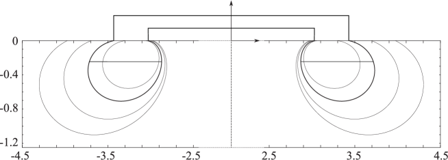
$\nu^{(\sigma)}x$ $\nu^{(\sigma)}y$ ballast ${\cal S}_{-}$ ballast ${\cal S}_{+}$

Figure 2: Level lines of the stream function $\psi_{0}$ plotted in non-dimensional coordinates. An example of the wetted contours bounding a motionless trapping body is shown in bold and denoted by ${\cal S}_{-}$ and ${\cal S}_{+}$; other pairs of symmetric streamlines can also be considered as boundaries of immersed parts of trapping bodies. In order to contract the width of the figure, a reduced horizontal scale is applied on the interval (-2.5, 2.5).

The trace $\psi_{0}(\nu^{(\sigma)}x,0)$ has only one positive zero $\nu^{(\sigma)}x_{0}\in\big{(}\frac{2\pi}{3},\pi\big{)}$ and

$$\psi_{0}(\nu^{(\sigma)}x,0)<0\quad\mbox{on}\ (0,\nu^{(\sigma)}x_{0}).$$

Moreover, this function increases monotonically from $0$ to $+\infty$ on $\left[\nu^{(\sigma)}x_{0},\pi\right)$ and decreases monotonically from $+\infty$ to $0$ on $\left(\pi,+\infty\right)$. Therefore, for every non-dimensional $d>0$ the streamline ${\cal S}_{+}=\big{\{}(\nu^{(\sigma)}x,\nu^{(\sigma)}y)\in\overline{\mathbb{R}^{2}_{-}}:\,x>0,\,y<0,\,\psi_{0}(\nu^{(\sigma)}x,\nu^{(\sigma)}y)=d\big{\}}$ (see the right part of figure 2) connects two points that lie on the positive $\nu^{(\sigma)}x$-axis on either side of the point $(\pi,0)$ at which $\psi_{0}$ is infinite.

Thus, for the chosen $\omega$ and every $d>0$ the domain $B_{+}$ between

$$S_{+}=\left\{(x,y)\in\overline{\mathbb{R}^{2}_{-}}:(\nu^{(\sigma)}x,\nu^{(\sigma)}y)\in{\cal S}_{+}\right\}$$

and the $x$-axis serves as the right immersed part of a single motionless trapping body $\widehat{B}$ obtained by connecting $B_{+}$ with the symmetric domain $B_{-}$ as shown in figure 2 for the corresponding domains in non-dimensional variables. Indeed, the Cauchy–Riemann equations imply that $\varphi_{0}$ satisfies the homogeneous Neumann condition on $S=S_{-}\cup S_{+}$, and so the coupling condition (4) is fulfilled for the mode $(\varphi_{0},(\bm{0},0)^{\mathsf{T}})$. The coupling condition (6) is also fulfilled for this mode because it reduces to the equality

$$\int_{S_{-}\cup S_{+}}\varphi_{0}\,n_{y}\,\mathrm{d}\kern 0.2pts=0\,.$$

Indeed, the other two equalities are trivial by the symmetry of $S_{-}\cup S_{+}$ and the fact that the corresponding integrands are odd functions of $x$. The proof that the last integral vanishes is based on the second Green’s formula and the asymptotic formulae (18) (see details in [3]).

4.2 The effect of the brash ice on motionless trapping bodies

The procedure described in §4.1 rigorously establishes the existence of trapping bodies, but it does not present pictorially the effect of the brash ice, that is, how these bodies differ from those trapping waves in the open water. In order to do this, we apply rescaling of specially chosen contours from the non-dimensional coordinates $(\nu^{(\sigma)}x,\nu^{(\sigma)}y)$ to $(\nu x,\nu y)$ for which purpose the equality $\nu=\nu^{(\sigma)}/(1+\sigma\nu^{(\sigma)})$ serves. Rescaling can be realised in two different manners — by keeping the area of the immersed part fixed and by keeping the length of $D$ fixed. The corresponding results are shown in figures 3 and 4 respectively, where three values of frequency are considered to demonstrate the effect; the frequency is characterised by the product $\nu\sigma$.

In figures 3 and 4 (a)–(c), examples of symmetric bodies trapping waves in the water covered by the brash ice are shown. The bodies are represented by the boundaries of their right immersed parts; see the left contour in each figure (cf. figure 2, where an example of the whole body is shown in the non-dimensional coordinates $(\nu^{(\sigma)}x,\nu^{(\sigma)}y)$). The location of the body that traps waves in the open water at the same frequency is indicated for comparison; it is plotted in bold (see the contour on the right-hand side of each figure). Both bodies have either the same area of the immersed part (the scaling adopted in figure 3) or the same length of $D$ (the scaling adopted in figure 4). The dashed lines in figures 3 (b) and 4 (b) show the contours from which the left ones are obtained by the scaling $(\nu^{(\sigma)}x,\nu^{(\sigma)}y)\mapsto(\nu x,\nu y)$.

Thus, figures 3 (a)–(c) demonstrate the following properties of the obtained symmetric trapping bodies with the fixed immersed area. The spacing between two immersed parts is less for bodies that trap waves in the water covered by the brash ice than for bodies that trap waves in the open water. Moreover, this spacing decreases as the frequency of trapped waves increases, whereas the length of $D$, on the opposite, increases together with the frequency.

The properties of symmetric trapping bodies with the fixed length of $D$ are as follows; see figures 4 (a)–(c). The spacing between two immersed parts demonstrates the same behaviour as in the other case, whereas the immersed area decreases as the frequency increases.

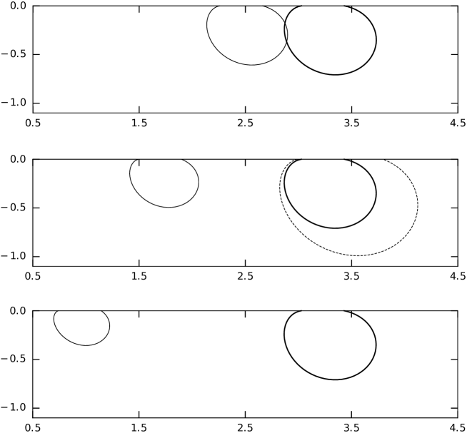
$\nu x$ $\nu y$ $\nu x$ $\nu y$ $\nu x$ $\nu y$ $(a)$ $(b)$ $(c)$

Figure 3: Examples of bodies trapping waves in the water covered by the brash ice for $\nu\sigma=1/4$ (a); $\nu\sigma=1/2$ (b); $\nu\sigma=3/4$ (c). In each figure, the left contour is the right immersed part of a symmetric body trapping waves; the bold contour shows the location of the body that has the same length of $D$ and traps waves in the open water at the same frequency. The dashed line in figure (b) shows the contour from which the left one is obtained by the scaling $(\nu^{(\sigma)}x,\nu^{(\sigma)}y)\mapsto(\nu x,\nu y)$.

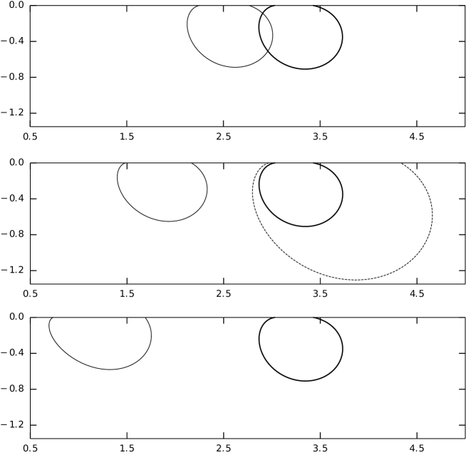
$\nu x$ $\nu y$ $\nu x$ $\nu y$ $\nu x$ $\nu y$ $(a)$ $(b)$ $(c)$

Figure 4: Examples of bodies trapping waves in the water covered by the brash ice for $\nu\sigma=1/4$ (a); $\nu\sigma=1/2$ (b); $\nu\sigma=3/4$ (c). In each figure, the left contour is the right immersed part of a symmetric body trapping waves; the bold contour shows the location of the body that has the same area and traps waves in the open water at the same frequency. The dashed line in figure (b) shows the contour from which the left one is obtained by the scaling $(\nu^{(\sigma)}x,\nu^{(\sigma)}y)\mapsto(\nu x,\nu y)$.

5 The effect of the brash ice when $\bm{\nu\sigma\geq 1}$

Let $\widehat{B}$ be a freely floating body, that is, it satisfies all subsidiary conditions of §2. For the matrices $\bm{E}$ and $\bm{K}$ corresponding to $\widehat{B}$ (see (7) and the following formulae that define the matrices’ elements), we denote by $\lambda_{*}$ the largest $\lambda$ such that $\det(\lambda\bm{E}-\bm{K})=0$.

Proposition 2.

Let $(\varphi,\bm{\chi})\in H^{1}(W)\times\mathbb{R}^{3}$ be a solution of problem (2)–(6). If $\omega$ is such that $\nu\geq\max\{\lambda_{*},\sigma^{-1}\}$, where $\lambda_{*}$ corresponds to $\widehat{B}$ through $\bm{E}$ and $\bm{K}$, then $(\varphi,\bm{\chi})$ is a trivial solution.

Proof.

Let $R_{\alpha,\beta}=\{(x,y)\in\mathbb{R}^{2}_{-}:|x|<\alpha,\ y>-\beta\}$, where $\alpha,\beta>0$ are sufficiently large; for example, such that $B\subset R_{\alpha-1,\beta-1}$. Applying the first Green’s formula, we write

$$\int_{W\cap R_{\alpha,\beta}}\!\!\!\!\!\!\!\!|\nabla\varphi|^{2}\,\mathrm{d}\kern 0.2ptx\mathrm{d}\kern 0.2pty=\int_{S}\varphi\,\mathchoice{\raise-0.5pt\hbox{$\partial$}\vphantom{\partial}_{\mkern-1.5mu\bm{n}}^{\mkern 0.4mu}\mkern 0.3mu}{\raise-0.5pt\hbox{$\partial$}\vphantom{\partial}_{\mkern-1.5mu\bm{n}}^{\mkern 0.4mu}\mkern 0.3mu}{\raise-0.5pt\hbox{$\scriptstyle\partial$}\vphantom{\partial}_{\mkern-1.7mu\bm{n}}\mkern 0.1mu}{\raise-0.5pt\hbox{$\scriptscriptstyle\partial$}\vphantom{\partial}_{\mkern-1.7mu\bm{n}}\mkern 0.1mu}\varphi\,\mathrm{d}\kern 0.2pts+\int_{-\alpha}^{\alpha}[\varphi(x,y)\,\mathchoice{\raise-0.5pt\hbox{$\partial$}\vphantom{\partial}_{\mkern-1.5muy}^{\mkern 0.4mu}\mkern 0.3mu}{\raise-0.5pt\hbox{$\partial$}\vphantom{\partial}_{\mkern-1.5muy}^{\mkern 0.4mu}\mkern 0.3mu}{\raise-0.5pt\hbox{$\scriptstyle\partial$}\vphantom{\partial}_{\mkern-1.7muy}\mkern 0.1mu}{\raise-0.5pt\hbox{$\scriptscriptstyle\partial$}\vphantom{\partial}_{\mkern-1.7muy}\mkern 0.1mu}\varphi(x,y)]_{y=-\beta}^{y=0,x\in F}\,\mathrm{d}\kern 0.2ptx$$

$$+\int_{-\beta}^{0}[\varphi(x,y)\,\mathchoice{\raise-0.5pt\hbox{$\partial$}\vphantom{\partial}_{\mkern-1.5mux}^{\mkern 0.4mu}\mkern 0.3mu}{\raise-0.5pt\hbox{$\partial$}\vphantom{\partial}_{\mkern-1.5mux}^{\mkern 0.4mu}\mkern 0.3mu}{\raise-0.5pt\hbox{$\scriptstyle\partial$}\vphantom{\partial}_{\mkern-1.7mux}\mkern 0.1mu}{\raise-0.5pt\hbox{$\scriptscriptstyle\partial$}\vphantom{\partial}_{\mkern-1.7mux}\mkern 0.1mu}\varphi(x,y)]_{x=-\alpha}^{x=\alpha}\,\mathrm{d}\kern 0.2pty,$$ (20)

where the Laplace equation is taken into account. The assumptions imposed on $\varphi$ yield that: 1) there exists a sequence $\{\alpha_{k}\}_{k=1}^{\infty}$ such that $\alpha_{k}\to\infty$ as $k\to\infty$ and the last integral with $\beta=\infty$ and $\alpha=\alpha_{k}$ tends to zero as $k\to\infty$; 2) for all $\alpha>0$ we have that $\int_{-\alpha}^{\alpha}[\varphi(x,-\beta)\,\mathchoice{\raise-0.5pt\hbox{$\partial$}\vphantom{\partial}_{\mkern-1.5muy}^{\mkern 0.4mu}\mkern 0.3mu}{\raise-0.5pt\hbox{$\partial$}\vphantom{\partial}_{\mkern-1.5muy}^{\mkern 0.4mu}\mkern 0.3mu}{\raise-0.5pt\hbox{$\scriptstyle\partial$}\vphantom{\partial}_{\mkern-1.7muy}\mkern 0.1mu}{\raise-0.5pt\hbox{$\scriptscriptstyle\partial$}\vphantom{\partial}_{\mkern-1.7muy}\mkern 0.1mu}\varphi(x,-\beta)]\,\mathrm{d}\kern 0.2ptx\to 0$ as $\beta\to\infty$. Passing to the limit in (20), first as $\beta\to\infty$ and then as $\alpha_{k}\to\infty$, we obtain

$$\int_{W}|\nabla\varphi|^{2}\,\mathrm{d}\kern 0.2ptx\mathrm{d}\kern 0.2pty-\int_{F}\varphi(x,0)\,\mathchoice{\raise-0.5pt\hbox{$\partial$}\vphantom{\partial}_{\mkern-1.5muy}^{\mkern 0.4mu}\mkern 0.3mu}{\raise-0.5pt\hbox{$\partial$}\vphantom{\partial}_{\mkern-1.5muy}^{\mkern 0.4mu}\mkern 0.3mu}{\raise-0.5pt\hbox{$\scriptstyle\partial$}\vphantom{\partial}_{\mkern-1.7muy}\mkern 0.1mu}{\raise-0.5pt\hbox{$\scriptscriptstyle\partial$}\vphantom{\partial}_{\mkern-1.7muy}\mkern 0.1mu}\varphi(x,0)\,\mathrm{d}\kern 0.2ptx=\int_{S}\varphi\,\mathchoice{\raise-0.5pt\hbox{$\partial$}\vphantom{\partial}_{\mkern-1.5mu\bm{n}}^{\mkern 0.4mu}\mkern 0.3mu}{\raise-0.5pt\hbox{$\partial$}\vphantom{\partial}_{\mkern-1.5mu\bm{n}}^{\mkern 0.4mu}\mkern 0.3mu}{\raise-0.5pt\hbox{$\scriptstyle\partial$}\vphantom{\partial}_{\mkern-1.7mu\bm{n}}\mkern 0.1mu}{\raise-0.5pt\hbox{$\scriptscriptstyle\partial$}\vphantom{\partial}_{\mkern-1.7mu\bm{n}}\mkern 0.1mu}\varphi\,\mathrm{d}\kern 0.2pts.$$ (21)

Here the integral over $F$ vanishes when $\nu=\sigma^{-1}$ (in this case, the boundary condition (3) reduces to $\varphi=0$ on $F$); if $\nu>\sigma^{-1}$, this integral is equal to $\nu^{(\sigma)}\int_{F}[\varphi(x,0)]^{2}\,\mathrm{d}\kern 0.2ptx$, which is a consequence of (8). In both cases, the left-hand side of (21) is positive for a non-trivial $\varphi$ (in the second case, because $\nu^{(\sigma)}<0$).

On the other hand, it follows from (4) and (6) that

$$\int_{S}\varphi\,\mathchoice{\raise-0.5pt\hbox{$\partial$}\vphantom{\partial}_{\mkern-1.5mu\bm{n}}^{\mkern 0.4mu}\mkern 0.3mu}{\raise-0.5pt\hbox{$\partial$}\vphantom{\partial}_{\mkern-1.5mu\bm{n}}^{\mkern 0.4mu}\mkern 0.3mu}{\raise-0.5pt\hbox{$\scriptstyle\partial$}\vphantom{\partial}_{\mkern-1.7mu\bm{n}}\mkern 0.1mu}{\raise-0.5pt\hbox{$\scriptscriptstyle\partial$}\vphantom{\partial}_{\mkern-1.7mu\bm{n}}\mkern 0.1mu}\varphi\,\mathrm{d}\kern 0.2pts=\omega\bm{\chi}^{\mathsf{T}}\int_{S}\varphi\,\bm{N}\,\mathrm{d}\kern 0.2pts=-g^{-1}\bm{\chi}^{\mathsf{T}}[\nu\bm{E}-\bm{K}]\bm{\chi}\,,$$

and so the right-hand side term of (21) is non-positive when $\nu\geq\lambda_{*}$. Thus, this contradicts to the positivity of the left-hand side with a non-trivial $\varphi$ when $\nu\geq\max\{\lambda_{*},\sigma^{-1}\}$. This completes the proof of the proposition. ∎

6 Concluding remarks

This note extends our previous work on motionless trapping bodies. Here, it has been shown that there exist two-dimensional bodies with a vertical axis of symmetry and two immersed parts and the following properties. These bodies are freely floating but motionless and trap some time-harmonic modes provided their frequencies are bounded by a constant characterising the brash ice. Thus, there is a coupled motion of the water covered by this ice that does not radiate waves to infinity in the presence of such a body. Therefore, in the absence of viscosity, this oscillation will persist forever.

On the other hand, for every freely floating body there exists a bound for frequencies (it depends also on the constant that characterises the brash ice) such that no modes are trapped at the frequencies exceeding this bound. Unlike uniqueness theorems known hitherto and concerning time-harmonic waves in the presence of freely floating bodies, this result does not involve any geometric restrictions.

References

• [1] Gabov, S. A., Sveshnikov, A. G. 1991 Problems in the dynamics of flotation liquids. J. Sov. Math. 54, 979–1041.
• [2] John, F. 1949 On the motion of floating bodies, I. Comm. Pure Appl. Math. 2, 13–57.
• [3] Kuznetsov, N. 2011 On the problem of time-harmonic water waves in the presence of a freely-floating structure. St Petersburg Math. J. 22, 985–995.
• [4] Kuznetsov, N. 2015 Two-dimensional water waves in the presence of a freely floating body: trapped modes and conditions for their absence. J. Fluid Mech. 779, 684–700.
• [5] Kuznetsov, N., Maz’ya, V., Vainberg, B. 2002 Linear water waves: a mathematical approach, Cambridge University Press.
• [6] Kuznetsov, N., Motygin, O. 2011 On the coupled time-harmonic motion of water and a body freely floating in it. J. Fluid Mech. 679, 616–627.
• [7] Kuznetsov, N., Motygin, O. 2012 On the coupled time-harmonic motion of deep water and a freely floating body: trapped modes and uniqueness theorems. J. Fluid Mech. 703, 142–162.
• [8] Kuznetsov, N., Motygin, O. 2015 Freely floating structures trapping time-harmonic water waves. Quart. J. Mech. Appl. Math. 68, 173–193.
• [9] Linton, C. M., McIver, P. 2001 Handbook of Mathematical Techniques for Wave/Structure Interactions, Chapman & Hall/CRC.
• [10] Peters, A. S. 1950 The effect of a floating mat on water waves. Comm. Pure Appl. Math. 3, 319–354.