Quantum and Thermal Fluctuations and Pair-breaking in Planar QED

Abstract

Planar quantum electrodynamics, in presence of tree-level Chern-Simons term, is shown to support bound state excitations, with a threshold, not present for the pure Chern-Simons theory. In the present case, the bound state gets destabilized by vacuum fluctuations. The bound state itself finds justification in the duality of the theory with massive topological vector field. Thermal fluctuations further destabilize this state, leading to smooth dissociation at high temperatures. Physical systems are suggested for observing such a bound state.

1 Introduction

Planar Chern-Simons (CS) electrodynamics yields an exact, weakly-bound, particle-antiparticle bound state (exciton), both in the relativistic H and non-relativistic H2 regimes. Summation of the bubble diagrams leads to this non-perturbative effect, wherein the binding energy H ,

$$\epsilon\approx\exp\left(-4\pi\frac{|m|}{m}\mu/e^{2}\right),$$ (1)

with CS coefficient $\mu$, fermion mass $m$ and coupling strength $e$. It is strikingly similar to the gap of superconductivity $|\Delta|\approx 2\omega_{D}\exp\left[\frac{1}{\pi\nu(0)\lambda}\right],~{}~{}~{}\lambda<0$ Schakel , where $\omega_{D}$ is the Debye frequency, and $\nu(0)$ is the density of states. Pure CS QED is devoid of any dynamics, and only affects the statistics of the interacting particles H2 . Coupling to the matter field leads to kinetic terms for the gauge field, which are sub-dominant in the low-energy limit, being second order in derivative. However, originating from the vacuum-fluctuations of the matter particles, the same is expected to destabilize the above bound state. Here, we investigate the role of quantum and thermal fluctuations in pair-breaking through the non-perturbative Schwinger-Dyson equation (SDE) SDE ; SDE1 ; IZ , from the analytical structure of the full quantum propagator.

In addition to the Maxwell Lagrangian, the presence of the CS term,

$$\mathcal{L}_{CS}:=\frac{\mu}{2}\epsilon^{\mu\nu\rho}a_{\mu}\partial_{\nu}a_{\rho},$$

at tree level, makes the theory ‘massive’, while preserving the gauge-invariance of the field $a_{\mu}$ TopM1 ; TopM11 ; TopM2 ; TopM22 ; Red ; Red1 . Consequently, the spins of both gauge ($\mu/|\mu|$) and fermion ($m/2|m|$) emerges TopM2 ; TopM22 ; Boy ; Boy1 , which are dependent on the fermion mass $m$. The topological CS term, that breaks parity, can arise through quantum corrections, owing to interactions with both bosonic pkp02 and fermionic TopM1 ; TopM11 ; TopM2 ; TopM22 ; Red ; Red1 ; Boy ; Boy1 ; Appel ; H fields, containing parity-breaking terms. In 2+1 dimensions, the corresponding form factors logarithmically diverge at momentum equal to $2m$. Consequently, the pole of the full propagator from SDE, leads to a physical bound state just below the two-fermion threshold. The above 1-loop result, though approximate, is justified by large-N arguments Ren ; Inf , and also as the CS contribution does not arise beyond 1-loop CH .

Such quantum corrections, in general, additionally induces gauge dynamics, through the kinetic part $\propto F_{\mu\nu}F^{\mu\nu}$. This induces vacuum fluctuations in the gauge sector, reflected in the pole structure of the full gauge propagator, for the same value of the momentum. In this paper, we investigate the formation and subsequent stability of this bound state, in presence of both vacuum and thermal fluctuations. In the following, Section I deals with the bound state in presence of gauge dynamics, with the corresponding vacuum fluctuation shown to impose a finite parametric threshold for the existence of the topological bound state. This threshold is justified through the duality of the system with massive topological vector fields. The effect of thermal influence is dealt with in Section II, depicting smooth dissociation of the bound state at sufficiently high temperature, through generalization of existing results. We conclude with discussions and remarks, pointing-out possible physical realization of such exotic states.

2 Bound state in presence of vacuum fluctuations

Planar QED is defined by the Lagrangian,

$$\mathcal{L} = \bar{\psi}(x)\left(i\gamma^{\mu}\partial_{\mu}-m-\gamma^{\mu}a_{\mu}(x)\right)\psi(x)-\frac{1}{4}F_{\mu\nu}F^{\mu\nu}+\frac{\mu}{2}\epsilon^{\mu\nu\rho}a_{\mu}\partial_{\nu}a_{\rho},$$ (2)

$$\gamma^{\mu} = (\sigma_{3},i\sigma_{1},i\sigma_{2}),~{}~{}~{}\hbar=c=1,$$

with coupling constant $e$, where the Dirac algebra is defined by Pauli matrices TopM1 ; TopM11 ; TopM2 ; TopM22 ; H . One can employ the derivative expansion scheme DE ; DE1 ; DE2 ; DE3 , owing to smallness of the coupling constant with respect to the corresponding momentum scale. The dominant non-zero contribution comes at the second order, identified by the vacuum polarization tensor,

$$\Pi^{\mu\nu}(q) = ie^{2}T_{r}\int_{p}\left[\gamma^{\mu}S(p_{+})\gamma^{\nu}S(p_{-})+\gamma^{\mu}\frac{\partial}{\partial p_{\nu}}S(p)\right];$$

$$\int_{p} = \int\frac{d^{3}p}{(2\pi)^{3}},~{}~{}~{}S(p)=\left[\gamma^{\mu}p_{\mu}-m\right],$$

$$p_{\mu} = i\partial_{\mu},~{}~{}~{}p_{\pm}=p\pm\frac{q}{2},$$ (3)

modulo the normalization owing to the non-interacting fermionic contribution, with the Dirac trace eliminating the first order term. Here, $q$ is the external momentum of the gauge field. The second term in the integrand represents the Gotó-Imamura-Pradhan-Schwinger GI ; Pradhan ; Schwinger term, utilizing current as the limit including a gauge invariant exponential H , which essentially regularizes the linear UV divergence of planar vacuum polarization Ren . Hence, there is no need of additional gauge-invariant regularization (e.g., Pauli-Villars).

The evaluation of the above integral is straight-forward, which can be carried out both in Minkowski space (using Schwinger parametrization) G and in Euclidean space (using Feynman’s trick) NA3 ; Rao ; Rao01 followed by continuation back to the Minkowski space, both yielding the result:

$$\Pi^{\mu\nu}(q) \equiv \Pi_{e}(q)\left(q^{\mu}q^{\nu}-\eta^{\mu\nu}q^{2}\right)+\Pi_{o}(q)\epsilon^{\mu\nu\rho}q_{\rho},$$

$$\Pi_{e}(q) = \frac{e^{2}}{4\pi}\left[\frac{1}{|q|}\left(\frac{1}{4}+\frac{m^{2}}{q^{2}}\right)\log\left(\frac{2|m|+|q|}{2|m|-|q|}\right)-\frac{|m|}{q^{2}}\right],$$

$$\Pi_{o}(q) = -i\frac{m}{4\pi}\frac{e^{2}}{|q|}\log\left(\frac{2|m|+|q|}{2|m|-|q|}\right).$$ (4)

The parity-odd contribution $\Pi^{\mu\nu}_{o}(q)$ is special to 2+1 Red ; Red1 , absent in 3+1, which arises due to non-zero Dirac trace ($Tr_{D}$) of three gamma matrices. This is the induced Chern-Simons contribution at loop level, including the topological Lévi-Civita tensor. The parity-even contribution $\Pi^{\mu\nu}_{e}(q)$ is responsible for wave-function renormalization. The plots of both the form factors $\Pi_{e,o}(q)$ are shown in Fig. 1, with the well-known singularities at the two-particle threshold.

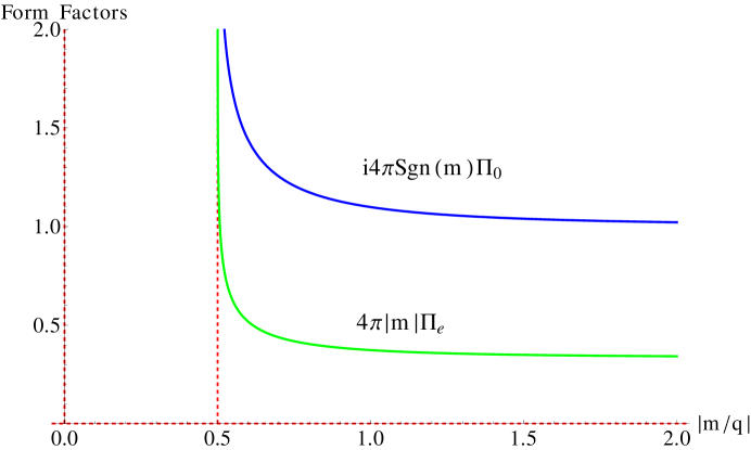
Figure 1: Plots of even and odd form factors of vacuum polarization tensor. Both the discontinuities, shown by red dashed lines, appear at two particle threshold, i.e., $|q|=2|m|$. Here $e^{2}=1$.

It is to be mentioned here that the results in Eqs. 4, which are valid for $q^{2}<4m^{2}$, are adopted as we are interested in pole(s) of the gauge propagator just below the two-fermion threshold. For $q^{2}>4m^{2}$, a branch-cut opens up owing to the singularity at $q^{2}>4m^{2}$, resulting into the replacement:

$$\log\left(\frac{2|m|+|q|}{2|m|-|q|}\right)\rightarrow\log\left(\frac{2|m|+|q|}{2|m|-|q|}\right)-i\pi,$$

in Eqs. 4.

In order to obtain the full gauge propagator, we consider the 1-loop SDE. The SDE, obtained by setting the variation of the generating functional $Z:=\int\mathcal{D}[\{\phi\}]\exp[i\int_{x}\mathcal{L}]$ with respect to the constituent fields ($\{\phi\}$s) equal to zero, is the equation of motion for the particular field IZ . In case of gauge fields, considering the Lagrangian of Eq. 2, the same turns out as,

$$\left[G_{F}^{\mu\nu}(q)\right]^{-1}=\left[G_{F}^{(0)~{}\mu\nu}(q)\right]^{-1}+\Pi^{\mu\nu}(q)-\frac{1}{\xi}q^{\mu}q^{\nu},$$ (5)

up to 1-loop. Here, $G_{F}^{\mu\nu}$ is the full gauge propagator and $G_{F}^{(0)~{}\mu\nu}(q)$ is the same at tree-level. We have separated out the contribution due to the covariant $R_{\xi}$ gauge in the last term, in order to incorporate different forms of tree level propagators through the above equation, subjected to different $\mathcal{L}_{g}$s. On inversion of the above SDE, the full propagator gets contribution from a class of diagrams made out of a number of vacuum polarization (bubble) terms, making the result non-perturbative IZ .

For the gauge Lagrangian in Eq. 2, with CS term accompanied by the kinetic term corresponding to the tree-level propagator,

$$G_{0}^{\mu\nu}=-\frac{1}{q^{2}-\mu^{2}}\left[\eta^{\mu\nu}-\frac{q^{\mu}q^{\nu}}{q^{2}}-i\frac{\mu}{q^{2}}\epsilon^{\mu\nu\rho}q_{\rho}\right]-\xi\frac{q^{\mu}q^{\nu}}{q^{4}},$$ (6)

the SDE leads to the 1-loop propagator Rao ; Rao01 ,

$$G^{\mu\nu}(q) \equiv\frac{1}{\left[q^{2}\{1+\Pi_{e}(q)\}^{2}+\left\{\Pi_{o}(q)+i\mu\right\}^{2}\right]q^{2}}$$

$$\times\left[\left(q^{\mu}q^{\nu}-\eta^{\mu\nu}q^{2}\right)\{1+\Pi_{e}(q)\}-\epsilon^{\mu\nu\rho}q_{\rho}\left\{\Pi_{o}(q)+i\mu\right\}\vphantom{\left(q^{\mu}q^{\nu}-\eta^{\mu\nu}q^{2}\right)}\right]$$

$$-\xi\frac{q^{\mu}q^{\nu}}{q^{4}}.$$ (7)

Apart from the usual pole at $q^{2}=0$, the above propagator has a non-trivial pole, defined by the solution of the equation,

$$q^{2}\{1+\Pi_{e}(q)\}^{2}+\left\{\Pi_{o}(q)+i\mu\right\}^{2}=0.$$ (8)

The pole of the gauge propagator, if local in the momentum space and gauge-invariant, represents a physical state of the system IZ . Though the latter criteria is satisfied, the prior is in general not true for the present case. However, just below the two-fermion threshold, parametrized by $|q|=2|m|-\epsilon$, with $|m|\gg\epsilon\cong 0$ the same is satisfied H . However, as this pole appears just below the two-particle threshold of the integrated-out fermions, this is an effective occurrence of a shallow fermionic bound state. The corresponding binding energy (BE) can be identified as,

$$\epsilon=4|m|\exp\left\{\frac{4\pi}{e^{2}}\left(2|m|-\mu\frac{m}{|m|}\right)\right\}.$$ (9)

A similar result was obtained by Hagen for pure CS QED, without gauge dynamics, yielding $\epsilon\approx\exp\left(-4\pi\frac{m}{|m|}\mu/e^{2}\right)$ H . There, the sign of fermion mass $\frac{m}{|m|}$, or the ‘induced’ photon spin TopM2 ; TopM22 ; Boy ; Boy1 in 2+1, has to be positive for $\mu>0$, and negative otherwise, for attaining a sensible (small) value of $\epsilon$. This is required for validity of the expansion, a fact not stressed upon in Ref. H . It is sensible that the BE disappears for $e^{2}\rightarrow 0$ (weak coupling limit).

In the present case, the presence of the kinetic term, representing vacuum fluctuations, opposes the formation of the bound state, against the CS influence, represented by the exponent in Eq. 9. Only beyond a critical value,

$$\mu\frac{m}{|m|}\equiv 2|m|:=\mu_{c},$$ (10)

of the CS coefficient, this exponent can be negative, provided the photon spin and $\mu$ have the same sign. Then the $\epsilon$-expansion is meaningful, and thereby corresponds to a shallow bound state.

At the tree-level, the sign of the CS coefficient $\mu$ gives the photon spin. The quantum effects shift the same as $\mu\rightarrow\mu-i\Pi_{o}(m,q)$ in the effective gauge Lagrangian. Due to the logarithmic singularity of $\Pi_{o}(m,q)$, at $|q|\rightarrow 2|m|$, it dominates $\mu$, yielding the ‘final’ induced photon spin: $m/|m|$ Own1 . Physically, the photon spin at the tree-level is substituted by the combined spin of the fermion-anti-fermion bound state in the effective theory, the latter ($\frac{m}{2|m|}$ each) being additive as spin is a $U(1)$ conserved quantity in 2+1 dimensions. To be a bound state, realized in the photon-channel, the bound state spin must be parallel to the original photon spin ($\mu/|\mu|$), necessitating the positivity of $\mu\frac{m}{|m|}$. In general, the relative sign of $\mu$ and the induced photon spin can be arbitrary ($\pm 1$) near the two-fermion threshold. Only when they have the same sign, the exciton can exist, provided the condition in Eq. 10 is satisfied.

Fig. 2 depicts the plot of Eq. 9 for three different values of $m$ in suitable units. The parametric region corresponding to physical bound state is observed.

2.1 The nature of the bound state

Since this bound state appears as a pole of the gauge propagator, it is charge-less, and dissociates into an electron-positron pair at the two particle threshold ($q^{2}=4m^{2}$). These assertions are confirmed by the corresponding 1-loop renormalization coefficients, large-N protected beyond 1-loop, that can be read-off from Eq. 7. The Lehmann weight,

$$Z_{3}=\left[1+\Pi_{e}(q)\right]^{-1}=\left[1+\frac{e^{2}}{4\pi}\left\{\frac{1}{|q|}\left(\frac{1}{4}+\frac{m^{2}}{q^{2}}\right)\log\left(\frac{2|m|+|q|}{2|m|-|q|}\right)-\frac{|m|}{q^{2}}\right\}\right]^{-1},$$ (11)

vanishes near the two-particle threshold, owing to the logarithmic singularity of Eq. 4, marking emergence of bound state IZ . Further, the renormalized charge $e^{2}_{r}=Z_{3}e^{2}$ vanishes in the same limit, asserting the state to be charge-less. This still renders the components to be a pair of particle and anti-particle, as in planar world, both species have the same spin orientation TopM1 ; TopM11 ; TopM2 ; TopM22 ; Boy ; Boy1 . Additionally, the renormalized topological mass,

$$\mu_{r} = \left[\mu-i\Pi_{o}(q)\right]Z_{3}$$ (12)

$$= \left[\mu-\frac{m}{4\pi}\frac{e^{2}}{|q|}\log\left(\frac{2|m|+|q|}{2|m|-|q|}\right)\right]$$

$$\times \left[1+\frac{e^{2}}{4\pi}\left\{\frac{1}{|q|}\left(\frac{1}{4}+\frac{m^{2}}{q^{2}}\right)\log\left(\frac{2|m|+|q|}{2|m|-|q|}\right)-\frac{|m|}{q^{2}}\right\}\right]^{-1},$$

leads to $\mu_{r}^{2}\geq 4m^{2}$ near the two-particle threshold, reflecting the threshold condition for the formation of the bound state.

Figure 2: Plots of BE $\epsilon$ against interaction strength $e$ and the CS coefficient $\mu$, for $|m|$ being $1$ (maroon), $1.5$ (green) and $2.5$ (blue) respectively (in natural units). Suitable regions for bound state formation (small $\epsilon$) exist for all three values, marked in red color, signifying the importance of the condition $\mu>2|m|$.

The topological origin of this bound state can be analogous to the finite boundary of the K-space of a superconductor, leading the expression of the corresponding gap. In the latter case, the order parameter $\Delta$ is introduced as an auxiliary interaction field, marking an additional energy scale in the system, that physically represents the BE of the Cooper-pair FW . However, this requires an underlying non-relativistic physics, represented by the Ginzburg-Landau (GL) theory FW , unlike the present case. Further, the critical temperature of the BCS theory satisfies $T_{c}\propto|\Delta|$, which is not the case here, as it will be shown that a melting temperature of the topological bound state cannot be evaluated exactly.

From Eq. 6, the tree-level gauge theory has mass equal to the CS coefficient itself TopM1 ; TopM11 ; TopM2 ; TopM22 ; Red ; Red1 . The quantum effects shift that pole to accommodate a bound state, with a lower-bound $\mu_{c}=2|m|$ on the topological mass magnitude (Eq. 9). As the form factors are of $\mathcal{O}(e^{2})$, expansion of Eq. 8 yields,

$$\mu^{2}=q^{2}+\frac{2}{|m|}\left[|m|\Pi_{e}+i\mu m\Pi_{o}\right],~{}~{}~{}\Pi_{o}\in\Im,~{}~{}\Pi_{e}\in\Re$$

As the term in the square bracket is a positive definite [Fig. 1], $\mu^{2}>q^{2}$ and near the two-particle threshold, $\mu^{2}>4m^{2}$. The bound-state vanishes also for $\mu^{2}\gg 4m^{2}$, as $\epsilon\rightarrow 0$.

2.2 Duality

The physical reason as to why the CS term allows for the bound state pole in the photon channel is of critical interest. More interestingly, destabilization effect due to vacuum fluctuations does not entirely eliminate the same, but only introduces a finite threshold for formation. This can be understood from the duality of the present theory with the massive CS vector field Equi ,

$$\mathcal{L}_{g}=\mu^{2}a^{\mu}a_{\mu}+\frac{\mu}{2}\epsilon^{\mu\nu\rho}a_{\mu}\partial_{\nu}a_{\rho},$$

with $\mu$ being the mass. They both yield essentially the same equation of motion, and are different constrained forms of a more extensive Lagrangian Equi . The corresponding tree-level propagators are related as,

$$iq^{\beta}\epsilon_{\beta\gamma\nu}\left(\tilde{G}_{0}^{-1}\right)^{\mu\nu} = \mu\left[\left(G_{0}^{-1}\right)^{\mu}_{~{}\gamma}+\frac{1}{\xi}q^{\mu}q_{\gamma}\right]~{}~{}~{}\text{and}$$

$$-i\epsilon_{\sigma\beta\mu}q^{\beta}\left(G_{0}^{-1}\right)^{\mu\nu} = \frac{q^{2}}{\mu}\left(\tilde{G}_{0}^{-1}\right)^{~{}\nu}_{\sigma}-\mu q^{\nu}q_{\sigma},$$ (13)

where $\tilde{G}_{0}$ corresponds to the non-dynamic CS QED, expressed as,

$$\tilde{G}_{0}^{\mu\nu}=-\frac{1}{q^{2}-\mu^{2}}\left[\eta^{\mu\nu}-\frac{1}{\mu^{2}}q^{\mu}q^{\nu}-i\frac{1}{\mu}\epsilon^{\mu\nu\rho}q_{\rho}\right].$$ (14)

The corresponding Lagrangians are connected through a gauge transformation, singular for $\mu=0$ Mukhi . This explains the singularity of $\tilde{G}_{0}^{\mu\nu}$ and the extra longitudinal degree of freedoms appearing in Eqs. 13. This tree level duality is robust to quantum corrections Equi in presence of interaction generating vacuum polarization, as,

$$0 = \left(\mu^{2}-q^{2}\Pi_{e}\right)^{2}+\left(\Pi_{o}-i\mu\right)^{2}q^{2},~{}~{}~{}\text{yielding},$$

$$\epsilon = 4|m|\exp\left[\frac{2\pi\mu}{e^{2}|m|}(2m-\mu)\right].$$ (15)

Though the pole equation is different, the condition for attaining a bound state is exactly the same as dynamic CS QED ($\mu^{2}>4m^{2}$). This can also be obtained through the transformations among the respective 1-loop corrected propagators, as in Eq. 13. This further confirms the physicality of the bound-state pole, as the ‘duality’ is essentially a contraction of the inverse propagator. Additionally, for the massive case, inclusion of quantum corrections still maintains the need of gauge-fixing after the gauge transformation.

Thus, the topologically massive gauge theory is equivalent to a genuinely massive pure topological theory in terms of the bound state. Exploiting this, as is clearer in the latter case, whenever the photon mass is above the two-particle threshold of the fermions, it transforms into electron-positron pair. When it is slightly below that (owing to quantum corrections), there is no pair production and the difference is the BE. This explains the lower-bound $\mu_{c}$ of the coefficient of the topological term magnitude in the dynamic CS-QED to be same as the physical mass of the dual massive theory at two-particle threshold.

3 Effect of Thermal Fluctuations

We adopt the imaginary time formalism DasFT to analyze the behavior of this bound state at finite temperature. The evaluation for vacuum polarization in this formalism, for $QED_{3}$ (planar QED Wick-rotated into the Euclidean space) was done for massless fermions in Ref. Dorey . We extend it to the case of $m\neq 0$, in a form more adaptive to our nomenclature, and show that the already known specific results, both at finite and zero-temperature are different limiting cases of the present case.

To this end, we adopt the following definition of vacuum polarization Dorey ,

$$\Pi^{\mu\nu}(q) = ie^{2}Tr_{D}\int_{p}\gamma^{\mu}S_{F}(p)\gamma^{\nu}S_{F}(p-q),$$

$$S_{F}(p) := \left[\gamma^{\mu}p_{\mu}-m\right],~{}~{}~{}p_{\mu}:=i\partial_{\mu},$$ (16)

where, in contrast with Eq. 3, we have left out the Schwinger regularization term for brevity. Upon the Wick rotation to the imaginary time, the fermion variables are,

$$p_{E} = (p_{3},\vec{p}),~{}~{}~{}p_{3}=(2n+1)\frac{\pi}{\beta},$$

$$p^{2}_{3} = -p^{2}_{0},~{}~{}~{}p^{2}_{E}=p^{2}_{3}+\vec{p}^{2}=-p^{2},$$

$$n = 0,\pm 1,\pm 2\ldots,~{}~{}~{}\beta=1/T,$$ (17)

and the boson variables are,

$$q_{E} = (q_{3},\vec{q}),~{}~{}~{}q_{3}=2r\frac{\pi}{\beta},$$

$$q^{2}_{3} = -q^{2}_{0},~{}~{}~{}q^{2}_{E}=q^{2}_{3}+\vec{q}^{2}=-q^{2}$$

$$r = 0,\pm 1,\pm 2\ldots,$$ (18)

The manifest co-variant projections of vacuum polarization tensor, in Euclidean space, are introduced as DasFT ,

$$\Pi^{\mu\nu}(q_{E},\beta) = \Pi_{A}(q_{E},\beta)A^{\mu\nu}(q_{E})+\Pi_{B}(q_{E},\beta)B^{\mu\nu}(q_{E}),$$

$$A^{\mu\nu}(q_{E}) := \left(\delta^{\mu 3}-\frac{q^{\mu}q^{3}}{q^{2}_{E}}\right)\frac{q^{2}_{E}}{\vec{q}^{2}}\left(\delta^{3\nu}-\frac{q^{3}q^{\nu}}{q^{2}_{E}}\right),$$

$$B^{\mu\nu}(q_{E}) := \delta^{\mu i}\left(\delta^{ij}-\frac{q^{i}q^{j}}{\vec{q}^{2}}\right)\delta^{j\nu},$$

$$A^{\mu\nu}+B^{\mu\nu} \equiv \delta^{\mu\nu}-\frac{q^{\mu}q^{\nu}}{q^{2}_{E}}\equiv\frac{1}{q^{2}}Q^{\mu\nu},~{}~{}~{}\delta^{\mu\nu}=-\eta^{\mu\nu}$$

The last line of above equations leads to the physical constraint that, at $T=0$,

$$\Pi_{A}(q_{E},T=0)=\Pi_{B}(q_{E},T=0)\equiv\Pi_{e}(q)$$ (19)

From the definitions, it is obtained that,

$$\Pi_{A}(q_{E},\beta) = \frac{q^{2}_{E}}{\vec{q}^{2}}\Pi^{00}(q_{E},\beta)~{}~{}\text{and}$$

$$\Pi_{B}(q_{E},\beta) = -\Pi^{ii}(q_{E},\beta)-\frac{q^{2}_{3}}{\vec{q}^{2}}\Pi^{00}(q_{E},\beta),$$ (20)

where repeated indices mean summation, unless mentioned otherwise.

Therefore it suffices to evaluate the temporal and spatial components of vacuum polarization tensor. First we will obtain those for the parity-even part, which is,

$$\Pi^{\mu\nu}_{e}(q) \equiv i2e^{2}\int_{0}^{1}dx\int_{p}\frac{1}{\left(p^{2}-a^{2}\right)^{2}}\left[2p^{\mu}p^{\nu}+2x(1-x)\left(q^{\mu}q^{\nu}-\eta^{\mu\nu}q^{2}\right)\right.$$

$$\qquad~{}~{}~{}~{}~{}~{}~{}~{}~{}-\left.\eta^{\mu\nu}\left(p^{2}-a^{2}\right)-(2x-1)\left(\eta^{\mu\nu}p.q-p^{\mu}q^{\nu}-p^{\nu}q^{\mu}\right)\right],$$

where we have utilized the Feynman integration trick with the shift $p\rightarrow p+xq$, and upon continuing to Euclidean space by the rules:

$$p_{0} = ip_{3},~{}~{}~{}p^{2}=-p^{2}_{E},~{}~{}~{}q^{2}=-q^{2}_{E},~{}~{}~{}p.q=-p_{E}.q_{E},$$

$$Q^{\mu\nu} = Q^{\mu\nu}_{E}=\delta^{\mu\nu}q^{2}_{E}-q^{\mu}q^{\nu},~{}~{}~{}a^{2}=a^{2}_{E}=m^{2}+x(1-x)q^{2}_{E},$$

$$\int\frac{dp_{3}}{2\pi} \rightarrow \frac{1}{\beta}\sum_{n=-\infty}^{\infty},~{}~{}~{}p_{3}=\frac{2\pi}{\beta}\left(n+X\right),~{}~{}~{}X:=\frac{1}{2}+xr.$$ (21)

With these definitions, one can express the temporal and spatial even form factors as,

$$\Pi^{00}(q_{E},\beta) =-2\frac{e^{2}}{\beta}\int_{0}^{1}dx\int\frac{d^{2}p}{(2\pi)^{2}}\left[S_{1}-2p^{2}_{3}S_{2}-2x(1-x)\vec{q}^{2}S_{2}-(2x-1)q_{3}S^{*}\right],~{}~{}~{}\text{\&}$$

$$\Pi^{ii}(q_{E},\beta) =-2\frac{e^{2}}{\beta}\int_{0}^{1}dx\int\frac{d^{2}p}{(2\pi)^{2}}\left[2x(1-x)\left(q^{2}_{E}+q^{2}_{3}\right)S_{2}-2a_{E}^{2}S_{2}-2p^{2}_{3}S_{2}+(2x-1)q_{3}S^{*}\right];$$

$$S_{i} =\sum_{n=-\infty}^{\infty}\frac{1}{\left[p^{2}_{E}+a^{2}_{E}\right]^{i}},~{}~{}i=1,2~{}~{}~{}\text{\&}~{}~{}~{}S^{*}=\sum_{n=-\infty}^{\infty}\frac{p_{3}}{\left[p^{2}_{E}+a^{2}_{E}\right]^{2}}.$$

For the massive fermion, the frequency sums followed by 2-momentum integrals yields,

$$\int\frac{d^{2}p}{(2\pi)^{2}}S_{1} =-\frac{1}{4\pi}\log\left|\frac{\sin\pi\left(X+\frac{i\beta m}{2\pi}\right)}{\sin\pi\left(X+\frac{i\beta a_{E}}{2\pi}\right)}\right|,~{}~{}~{}\int\frac{d^{2}p}{(2\pi)^{2}}S_{2}=\frac{\beta}{16\pi}\frac{1}{a_{E}}\Im\cot\pi\left(X+\frac{i\beta a_{E}}{2\pi}\right),$$

$$\int\frac{d^{2}p}{(2\pi)^{2}}S^{*} =\frac{\beta}{16\pi}\left[\sin(2\pi X)-\Re\cot\pi\left(X+\frac{i\beta a_{E}}{2\pi}\right)\right],$$

$$\int\frac{d^{2}p}{(2\pi)^{2}}p_{3}^{2}S^{*} =\frac{1}{4}\Im\left[\frac{\sin\pi\left(X+\frac{i\beta m}{2\pi}\right)\cos\pi\left(X-\frac{i\beta m}{2\pi}\right)}{\left|\sin\pi\left(X+\frac{i\beta m}{2\pi}\right)\right|^{2}}+\cot\pi\left(X+\frac{i\beta a_{E}}{2\pi}\right)\right].$$ (22)

Finally, from Eq. 19, the finite temperature ‘orthogonal’ form factors DasFT are obtained as,

$$\Pi_{A} =\frac{e^{2}q^{2}_{E}}{\beta\vec{q}^{2}}\int_{x}\left[\frac{1}{2\pi}\log\left|\frac{\sin\pi\left(X^{+}_{m}\right)}{\sin\pi\left(X^{+}_{a}\right)}\right|-\Im\left\{\cot\pi\left(X^{-}_{m}\right)+\cot\pi\left(X^{+}_{a}\right)\right\}\right]$$

$$+\frac{e^{2}}{8\pi}\int_{x}\left[2x(1-x)\frac{q^{2}_{E}}{a_{E}}\Im\cot\pi\left(X^{+}_{a}\right)+(2x-1)q_{3}\frac{q^{2}_{E}}{\vec{q}^{2}}\left\{\sin(2\pi X)-\Re\cot\pi\left(X^{+}_{a}\right)\right\}\right]~{}~{}~{}\text{\&}$$

$$\Pi_{B} =-\frac{e^{2}}{\beta}\int_{x}\left[\frac{1}{2\pi}\log\left|\frac{\sin\pi\left(X^{+}_{m}\right)}{\sin\pi\left(X^{+}_{a}\right)}\right|-\frac{q^{2}_{E}}{\vec{q}^{2}}\Im\left\{\cot\pi\left(X^{-}_{m}\right)+\cot\pi\left(X^{+}_{a}\right)\right\}\right]$$

$$+\frac{e^{2}}{8\pi}\int_{x}\left[-2\frac{m^{2}}{a_{E}}\Im\cot\pi\left(X^{+}_{a}\right)+(2x-1)q_{3}\left(2-\frac{q^{2}_{3}}{\vec{q}^{2}}\right)\left\{\sin(2\pi X)-\Re\cot\pi\left(X^{+}_{a}\right)\right\}\right];$$

$$X^{\pm}_{m} =X\pm\frac{i\beta m}{2\pi}~{}~{}~{}\text{and}~{}~{}~{}X^{\pm}_{a}=X\pm\frac{i\beta a_{E}}{2\pi}.$$ (23)

Here, the Schwinger term regularization has been adopted as appropriate. The $x$-integrals cannot be evaluated exactly, as is known. However, at zero temperature, the same is possible, and one obtains $\Pi_{A}=\Pi_{B}$ as required; modulo an additional term in $\Pi_{B}$, known to arise for fermion-antifermion pair of the loop having the same mass DasFT . The rest is same as the result given in Eq. 4, once the expressions are continued back to the Minkowski space through $q_{3}\rightarrow-iq_{0}$. Additionally, in Eqs. 23, terms with overall multiplicative factor $T=1/\beta$ have been separated from the rest for convenience. This is because, confirmed by a analysis in real time formalism, the $x$-integrals turn out to be temperature-independent in the high-temperature limit, as will be seen in the next subsection. Then, the dominant temperature dependent and independent parts become well-separated.

As for the Chern-Simons coefficient, following a similar treatment leads to,

$$\Pi_{o}(q_{E},\beta)\equiv i\frac{me^{2}}{4\pi}\int_{0}^{1}\frac{dx}{a_{E}}\Im\cot\pi\left(X+is\frac{\beta a_{E}}{2\pi}\right)$$ (24)

In the zero-temperature limit, the above expression goes to that of Eqs. 4 as required. Further, in the high temperature limit ($\beta\rightarrow 0$), the dominant $\mathcal{O}(\beta)$ term is independent of $q$, and is the same as that for $q=0$ BDP . These facts ensure the consistency of our derivation.

3.1 Results at high temperatures

Though the $x$-integrals in Eqs. 23 and 24 cannot be evaluated exactly, approximate expressions, in the high temperature limit $T\gg q,m$ TFT , can be obtained as,

$$\Pi_{A}(q,T) \approx \frac{T}{2\pi}e^{2}\log(2)\frac{|\frac{q}{q_{0}}|}{1-|\frac{q}{q_{0}}|^{2}}\left[1-\frac{2}{3}\frac{|\frac{q}{q_{0}}|^{2}}{1-|\frac{q}{q_{0}}|^{2}}\right]-q^{2}\Pi_{e}(q),$$

$$\Pi_{B}(q,T) \approx -\frac{T}{3\pi}e^{2}\log(2)\frac{|\frac{q}{q_{0}}|^{3}}{1-|\frac{q}{q_{0}}|^{2}}-q^{2}\Pi_{e}(q),~{}~{}~{}\Pi_{o}(q,T)\approx-i\frac{\beta e^{2}}{8\pi}m.$$ (25)

The even part of the vacuum polarization at finite temperature can be expressed as Weldon ,

$$\Pi^{\mu\nu}_{e}(q,T) = \Pi_{T}(q,\omega)P^{\mu\nu}+\Pi_{L}(q,\omega)R^{\mu\nu},$$ (26)

$$P^{\mu\nu} = \eta^{\mu\nu}-u^{\mu}u^{\nu}+\frac{\tilde{q}^{\mu}\tilde{q}^{\nu}}{Q^{2}},~{}~{}~{}R_{\mu\nu}=-\frac{1}{q^{2}Q^{2}}(Q^{2}u_{\mu}+\omega\tilde{q}_{\mu})(Q^{2}u_{\nu}+\omega\tilde{q}_{\nu}),$$

$$\omega = q.u,~{}~{}~{}Q^{2}=\omega^{2}-q^{2},~{}~{}~{}\tilde{q}^{\mu}=q^{\mu}-\omega u^{\mu}.$$

with $\Pi_{T}=\Pi_{A}+q^{2}\Pi_{e}$ and $\Pi_{L}=\Pi_{B}+q^{2}\Pi_{e}$. here, $u_{\mu}=(1,0,0)$ is the position vector defining the rest frame of the thermal bath DasFT . A straight-forward, but tedious calculation leads to the 1-loop corrected full thermal propagator as,

$$G^{\mu\nu}(q,T) \equiv a(q,T)\eta^{\mu\nu}+b(q,T)q^{\mu}q^{\nu}+c(q,T)u^{\mu}u^{\nu}$$

$$+ d(q,T)(q^{\mu}u^{\nu}+u^{\mu}q^{\nu})+e(q,T)\epsilon^{\mu\nu\rho}q_{\rho};$$

$$a(q,T) = \frac{\Pi_{T}-q^{2}\left(\Pi_{e}+1\right)}{\left[\Pi_{T}-q^{2}\left(\Pi_{e}+1\right)\right]^{2}+q^{2}\left(\Pi_{o}+i\mu\right)^{2}},$$

$$b(q,T) = \frac{\left[\Pi_{L}-q^{2}\left(\Pi_{e}+1\right)\right]+\frac{q_{0}^{2}}{\vec{q}^{2}}(\Pi_{T}-\Pi_{L})}{q^{2}\left[q^{2}\left(\Pi_{e}+1\right)-\Pi_{L}\right]}a(q,T)+\frac{\xi}{q^{4}},$$

$$c(q,T) = -\frac{q^{2}}{\vec{q}^{2}}\frac{(\Pi_{T}-\Pi_{L})}{\left[\Pi_{L}-q^{2}\left(\Pi_{e}+1\right)\right]}a(q,T),$$

$$d(q,T) = -\frac{q_{0}}{q^{2}}c(q,T),~{}~{}~{}e(q,T)=-\frac{\left(\Pi_{o}+i\mu\right)}{\Pi_{T}-q^{2}\left(\Pi_{e}+1\right)}a(q,T),$$ (27)

The above equations reveal two non-trivial poles of the full propagator, corresponding to the identities,

$$\Pi_{L}-q^{2}\left(\Pi_{e}+1\right) = 0~{}~{}~{}\text{and}$$

$$\left[\Pi_{T}-q^{2}\left(\Pi_{e}+1\right)\right]^{2}+q^{2}\left(\Pi_{o}+i\mu\right)^{2} = 0.$$ (28)

Near the two-fermion threshold, the above identities corresponds to the respective bound state binding energies as,

$$\epsilon \approx 4|m|\exp{\left\{-{\rm T}\frac{4\pi}{|m|}\Pi_{l}+16\pi\frac{|m|}{e^{2}}\right\}}~{}~{}~{}\text{\&}$$

$$\epsilon \approx 4|m|\exp{\left\{\frac{4\pi}{e^{2}}\left(2|m|-\mu\frac{m}{|m|}\right)-8\pi{\rm T}\Pi_{t}\left(2|m|+\mu\frac{m}{|m|}\right)^{-1}\right\}},$$ (29)

where $\Pi_{l,t}(q)=\Pi_{L,T}(q,{\rm T})/{\rm T}e^{2}$. Here, we have retained the ${\cal O}(e^{0})$ term, along-with the dominant ${\cal O}(e^{-2})$ contribution, as the prior carries the temperature-dependence. In contrast, only the ${\cal O}(e^{-2})$ terms were retained in the exponent for the zero-temperature case (Eq. 9). However, the temperature-dependent part can substantially contribute, as the form factor $\Pi_{t}$ can be large, as can be seen in Fig. 3. In the above, the first expression is unphysical, as in the on-shell domain of $|q|<|q_{0}|$, $\Pi_{l}$ is negative, marking increase in binding energy with temperature. However, the second one is physically sensible, as the scaled form factor $\Pi_{t}$ is positive on-shell, representing melting of the bound state (Fig. 3). This, however, requires the factor $\mu m/|m|$ to be positive, required for a physically sensible bound-state, as had been seen for the zero-temperature case. Further, this expression reverts back to the result in Eq. 9 for $T=0$, as physically expected. This makes sense, although the expression for $\Pi_{t}$ has been obtained in the high-temperature limit, where it is temperature-independent. Though its exact form is expected to show temperature-dependence, the temperature dependent parts of the functions in the integrands of Eqs. 23 (the logarithms and cotangents) vanish identically for $T=0$, justifying the recovery of Eq. 9. Further, the finite temperature contribution is expected to be finite for any finite value of $T$, as finite temperature effects do not introduce additional singularities to the overall form factors DasFT . Therefore, ${\rm T}\Pi_{t}$ should vanish for $T=0$.

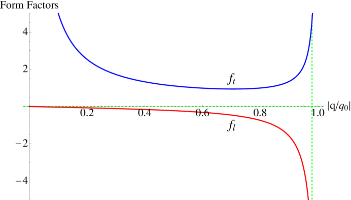
Figure 3: Plots of finite-temperature parts of coefficients of vacuum polarization tensor Vs. $|q/q_{0}|$. Here, $f_{l,t(q)}=2\pi\Pi_{l,t}(q)/\log(2)$. $f_{t}(q)$ is positive and hence is acceptable, within the physical region $0\leq|q/q_{0}|\leq 1$, whereas $f_{l}(q)$ is not.

Therefore, the finite temperature essentially does an exponential scaling of the electron-positron BE, under the high-$T$ approximation. Presently, the ‘critical’ temperature at which the bound state melts is not that straight-forward to obtain from this approximate approach. This exponential decay represents the destabilizing thermal fluctuations, as mentioned before, that lowers the BE than what it was at $T=0$. This shift may be observable in a physical system.

It has been shown that Grig 2+1 QED (without a tree-level CS term) shows confinement-deconfinement transition of Berezinskii-Kosterlits-Thouless (BKT) BKT ; BKT1 type. However, such a theory cannot account for a parity violating mass term and thus it emerges from the consideration of $4\times 4$ Dirac matrices, unlike the $2\times 2$ Pauli matrices as gamma matrices in the Dirac equation. This allows cancellation between the CS terms at the loop levels corresponding to particle and anti-particle sectors. Thus, it is imperative to note that in theories with topological terms and loop corrections are analyzed, possible phase transitions are not of BKT type. This also follows from the fact that BKT is an infinite order phase transition, unlike BCS phase transition, which is of second order and has analytic correspondence with the present theory.

4 Discussions and Remarks

The presence of both quantum and thermal fluctuations for gauge field destabilizes the fermion-antifermion bound state, with respect to the one for pure CS QED. The lower limit for the CS coefficient can signify a quantum ‘phase-transition’. It will be interesting to study the non-Abelian analogue of this model, as it also supports anomalies. The finite temperature treatment was demonstrated for massive fermions, which is consistent with the physical understanding of melting of the bound state. A first-quantized treatment of the model will be discussed in a following body of work, supporting complex angular momentum, resulting in Efimov-state-like resonances.

The fact that planar QED has manifested in effective low-energy theories of materials like graphene Own1 , with $U(1)$ gauge fields Ando01 and controlled mass gaps Hunt . The mono-layer graphene is described by relativistic fermions Gra2 , whereas the bi-layer one is governed by non-relativistic dynamics Neto . Formation of bound states in these systems and their controlled manipulation Own1 is of deep interest in the physical context. The manifest relativistic physics arise through emergent Dispersion in graphene Gra2 , wherein the fermion mass and coupling strength get scaled, respectively, as $m\rightarrow mv_{F}^{2}$ and $e\rightarrow ev_{F}\ll c$ Own1 by the Fermi velocity $v_{F}$, replacing the speed of light in vacuum ($c$) as a Lorentz invariant. The latter scaling makes the BE shallower, thereby increasing the sensitivity of the bound state to the parametric threshold. Further, the melting temperature of the bound state should not be lower than the range where the structure of these materials is intact, for the physical observation of the prior.

- (1) C. R. Hagen, A new gauge theory without an elementary photon, Ann. Phys. 157 (1984) 342.
- (2) C. R. Hagen, Rotational anomalies without anyons, Phys. Rev. D 31 (1985) 2135.
- (3) A. M. J. Schakel, Boulevard of Broken Symmetries: Effective Field Theories of Condensed Matter, World Scientific (2008).
- (4) F. Dyson, The Matrix in Quantum Electrodynamics, Phys. Rev. 75 (1949) 1736.
- (5) J. Schwinger, On the Green’s functions of quantized fields. I, PNAS 37 (1951) 452.
- (6) C. Itzykson and J.-B. Zuber, Quantum Field Theory, Courier Dover (2012).
- (7) J. F. Schonfeld, A mass term for three-dimensional gauge fields, Nucl. Phys. B 185 (1981) 157.
- (8) I. Affleck, J. Harvey and E. Witten, Instantons and (super-) symmetry breaking in (2+1) dimensions, Nucl. Phys. B 206 (1982) 413.
- (9) S. Deser, R. Jackiw and S. templeton, Three-Dimensional Massive Gauge Theories, Phys. Rev. Lett. 48 (1982) 975.
- (10) S. Deser, R. Jackiw and S. templeton, Topologically massive gauge theories, Ann. Phys. 140 (1982) 372.
- (11) A. Redlich, Gauge Noninvariance and Parity Nonconservation of Three-Dimensional Fermions, Phys. Rev. Lett. 52, 18 (1984).
- (12) A. Redlich, Parity violation and gauge noninvariance of the effective gauge field action in three dimensions, Phys. Rev. D 29, 2366 (1984).
- (13) D. Boyanovsky, R. Blankenbecler and R. Yahalom, Physical origin of topological mass in 2 + 1 dimensions, Nucl. phys. B 270 (1986) 483.
- (14) B. Binegar, Relativistic field theories in three dimensions, J. Math. Phys. 23 (1982) 1511.
- (15) C. R. Hagen, P. Panigrahi, and S. Ramaswamy, Still More Corrections to the Topological Mass, Phys. Rev. Lett. 61 (1988) 389.
- (16) T. W. Appelquist, M. Bowick, D. Karabali, and L. C. R. Wijewardhana, Spontaneous chiral-symmetry breaking in three-dimensional QED, Phys. Rev. D 33 (1986) 3704.
- (17) T. Appelquist and R. Pisarski, High-temperature Yang-Mills theories and three-dimensional quantum chromodynamics, Phys. Rev. D 23 (1981) 2305.
- (18) T. Appelquist and U. Heinz, Three-dimensional theories at large distances, Phys. Rev. D 24 (1981) 2169.
- (19) S. Coleman and B. Hill, No more corrections to the topological mass term in , Phys. Lett. B 159 (1985) 184.
- (20) V. A. Novikov, M. A. Shifman, A. I. Vainshtein and V. I. Zakharov, Calculations In External Fields In QCD: An Operator Method, Yad. Fiz. 39 (1984) 124 [Sov. J. Nucl. Phys. 39 (1984) 77].
- (21) C. M. Fraser, Calculation of Higher Derivative Terms in the One-Loop Effective Lagrangian, Z. Phys. C 28, 101 (1985).
- (22) L. -H. Chan, Phys. Rev. Lett. 54, 1222 (1985), Phys. Rev. Lett. 54 (1985) 1222.
- (23) J. A. Zuk, Functional approach to derivative expansion of the effective Lagrangian, Phys. Rev. D 32 (1985) 2653.
- (24) T. Gotó and T. Imamura, Note on the Non-Perturbation Approach to Quantum Field Theory, Prog. Theor. Phys. 14 (1955) 396.
- (25) T. Pradhan, On the one-dimensional spinor model of thirring, Nucl. Phys. 9 (1958) 124.
- (26) J. Schwinger, Field Theory Commutators, Phys. Rev. Lett. 3 (1959) 296.
- (27) W. Greiner and J. Reinhardt, Quantum Electrodynamics, Springer (1994).
- (28) R. Pisarski and S. Rao, Topologically massive chromodynamics in the perturbative regime, Phys. Rev. D 32 (1985) 2081.
- (29) S. Rao and R. Yahalom, Parity anomalies in gauge theories in 2 + 1 dimensions, Phys. Lett. B 172 (1986) 227.
- (30) P. Maris, Confinement and complex singularities in three-dimensional QED, Phys. Rev. D 52 (1995) 6087.
- (31) K. Abhinav and P. K. Panigrahi, Controlled Spin Transport in Planar Systems Through Topological Exciton, arXiv:1504.07955v3.
- (32) A. L. Fetter and J. D. Walecka, Quantum Theory of Many-Particle Systems, Dover Publications (2012).
- (33) S. Deser and R. Jackiw, “Self-duality" of topologically massive gauge theories, Phys. Lett. B 139 (1984) 371.
- (34) S. Mukhi, Unraveling the novel Higgs mechanism in (2+1)d Chern-Simons theories, JHEP 12 (2011) 83.
- (35) A. Das, Finite Temperature Field Theory, World Scientific (1999).
- (36) N. Dorey and N.E. Mavromatos, and two-dimensional superconductivity without parity violation, Nucl. Phys. B 386 (1992) 614.
- (37) K. S. Babu, A. Das and P. K. Panigrahi, Derivative expansion and the induced Chern-Simons term at finite temperature in 2+1 dimensions, Phys. Rev.D 36 (1987) 3725.
- (38) M. Le Bellac, Thermal Field Theory, Cambridge Monographs on Mathematical Physics, Cambridge University Press (2000).
- (39) H. A. Weldon, Covariant calculations at finite temperature: The relativistic plasma, Phys. Rev. D 26 (1982) 1394.
- (40) G. Grignani, G. Semenoff and P. Sodano, Confinement-deconfinement transition in three-dimensional QED, Phys. Rev. D 53 (1996) 7157.
- (41) V. L. Berezinksii, Destruction of Long-Range Order in One-Dimensions and Two-Dimensional Systems Possessing a Continuus Symmetry Group. II. Quantum Systems, Sov. Phys. JETP 34 (1972) 610 [Zh. E’ksp. Teor. Fiz. 61 (1972) 1144].
- (42) J. M. Kosterlitz and D.J. Thouless, Ordering, metastability and phase transitions in two-dimensional systems, J. Phys. C 6 (1973) 1181.
- (43) K. Ishikawa and T. Ando, Optical Phonon Interacting with Electrons in Carbon Nanotubes, J. Phys. Soc. Jpn. 75 (2006) 084713.
- (44) B. Hunt, J. D. Sanchez-Yamagishi, A. F. Young, M. Yankowitz, B. J. LeRoy, K. Watanabe, T. Taniguchi, P. Moon, M. Koshino, P. Jarillo-Herrero, and R. C. Ashoori, Massive Dirac Fermions and Hofstadter Butterfly in a van der Waals Heterostructure, Science 340 (2013) 1427.
- (45) G. W. Semenoff, Condensed-Matter Simulation of a Three-Dimensional Anomaly, Phys. Rev. Lett. 53 (1984) 2449.
- (46) A. H. C. Neto, F. Guinea, N. M. R. Peres, K. S. Novoselov and A. K. Geim, The electronic properties of graphene, Rev. Mod. Phys. 81 (2009) 109.