Study of statistical properties of hybrid statistic in coherent multi-detector CBC Search

Abstract

In this article, we revisit the problem of coherent multi-detector search of gravitational wave from compact binary coalescence with Neutron stars and Black Holes using advanced interferometers like LIGO-Virgo. Based on the loss of optimal multi-detector signal-to-noise ratio (SNR), we construct a hybrid statistic as a best of maximum-likelihood-ratio(MLR) statistic tuned for face-on and face-off binaries. The statistical properties of the hybrid statistic is studied. The performance of this hybrid statistic is compared with that of the coherent MLR statistic for generic inclination angles. Owing to the single synthetic data stream, the hybrid statistic gives low false alarms compared to the multi-detector MLR statistic and small fractional loss in the optimum SNR for a large range of binary inclinations. We have demonstrated that for a LIGO-Virgo network and binary inclination $\epsilon<70^{\circ}$ and $\epsilon>110^{\circ}$, the hybrid statistic captures more than $98\%$ of network optimum matched filter SNR with low false alarm rate. The Monte-Carlo exercise with two distributions of incoming inclination angles namely, $U[\cos\epsilon]$ and more realistic distribution proposed in Schutz (2011) are performed with hybrid statistic and gave $\sim 5\%$ and $\sim 7\%$ higher detection probability respectively compared to the two stream multi-detector MLR statistic for a fixed false alarm probability of $10^{-5}$.

I Introduction

On $14^{th}$ September 2015, the two Advanced LIGO detectors (LIGO-Livingston and LIGO-Hanford)Collaboration et al. (2015); Harry (2010) detected gravitational waves (GW) for the first time from a binary black hole merger eventAbbott et al. (2016). The Advanced Virgo detector will be ready for observation of cosmos very soonAcernese et al. (2015); The Virgo Collaboration (2012). The Japanese cryogenic detector KAGRA is under constructionAso et al. (2013); Somiya (2012) and proposal for a detector in India namely LIGO-India is in placeLIG (2011). Compact binary coalescences (CBC) with Neutron stars (NS) and Black Holes (BH) are one of the most promising GW sources for the Advanced LIGO-Virgo interferometric GW detectors. The Advanced LIGO detectors have a proposed distance reach of $\sim 445Mpc.$ for binary neutron star (BNS) events and are expected to detect few events of BNS inspiral per monthAbadie et al. (2010). Detection of CBC would reveal information about the BH as well as the NS equation of state. We expect many more surprises from nature in the form of GW detections which would emerge into a new, exciting field of GW astronomy in few decades.

The detection of GW in the interferometric data $\mathbf{x}$ is a statistical hypothesis testing problem, where the null hypothesis – $\mathbf{x}$ is purely noise $\mathbf{n}$ – is tested against an alternative hypothesis – $\mathbf{x}$ is signal $\mathbf{s}$ plus the noise $\mathbf{n}$. The decision is based on construction of a detection statistic – a real valued function of $\mathbf{x}$ – and is compared with a predefined threshold. When this test statistic crosses the threshold, the detection is declared. There are various strategies adopted for setting this threshold. The common strategy is to fix the false alarm rate (based on the available prior knowledge of the interferometer noise) and obtain the threshold value for the statistic.

The Neyman - Pearson lemmaHelstrom (1960) says, the likelihood ratio (LR) – the probability ratio of the data following alternative hypothesis and the null hypothesis – is the most power full test statistic in case of simple hypotheses (signal is known). However, in GW detection problem e.g. CBC search or continuous wave search (from a periodic source such as Pulsar), the signal model is known but the parameters are unknown. Here, the alternative hypothesis is a composite hypothesis. There are two approaches to composite hypothesis testing. The first approach is the maximum likelihood ratio (MLR) approach, where LR is maximized over the signal parameters. In the second approach – Bayesian approach – which includes the astrophysical priors of signal parameters, the LR is marginalized over the signal parameters with a prior distribution. For high signal-to-noise ratio (SNR), the LR is expected to peak at the actual signal values in the multi-dimensional space of signal parameters. Thus, most of the contribution to the marginalized LR is from the maximum. Therefore, the MLR statistic performs equally well as the marginalized statistic in the regime of high SNR.

The coherent multi-detector search of GW combines the incoming GW signal at different interferometers in a phase coherent way, where the information of the arrival time is incorporated in the phase. The MLR based multi-detector approach for CBC signals is developed in GW literature Pai et al. (2001); Harry and Fairhurst (2011); Haris and Pai (2014). The non-spinning CBC signal is a function of 9 parameters; namely masses, source location, amplitude, binary inclination, polarization angle, phase at the time of arrival and time of arrival at the reference detector. The MLR multi-detector statistic obtained by maximizing multi-detector LR over a subset of 4 signal parameters (namely; amplitude, binary inclination, polarization angle and initial phase) was shown to be the sum of MLR statistic of two synthetic data streams which captures the two GW polarizations in Einsteinian General Relativity. Henceforth, we would refer to this statistic as generic MLR statistic. In Williamson et al. (2014), authors investigate the performance of multi-detector MLR statistic devised for face-on/off binaries in the targeted follow-up of short gamma ray burst (SGRB) in the GW window. In Littenberg and Cornish (2009), authors explore Bayesian framework to address the multi-detector CBC detection problem. The multi-detector coherent approach for continuous wave search is developed in Cutler and Schutz (2005) and in Prix and Krishnan (2009), authors further compare the performance of Bayesian vs MLR statistic in a specific set of amplitude coordinates given in Jaranowski et al. (1998).

In this paper, we revisit the MLR based multi-detector CBC statistics. As mentioned above, the generic multi-detector MLR statistic, $\mathcal{L}$ for CBC signal is a sum of two single streams (synthetic data systems) MLR statistics (Eq.(2.38) of Harry and Fairhurst (2011) and Eq.(44) of Haris and Pai (2014)) in dominant Polarization frameKlimenko et al. (2005). In this work, we carefully analyze the statistical properties of multi-detector MLR statistic for Gaussian noise. Further, we obtain the MLR based statistics specially targeted for the face-on/off binaries which we denote as $\mathcal{L}^{0,\pi}$. This is a single data stream MLR statistic as opposed to the two stream $\mathcal{L}$ statistic and gives less false alarm rate as compared to that of $\mathcal{L}$. A careful study of SNRs of $\mathcal{L}^{0,\pi}$ indicate that either $\mathcal{L}^{0}$ or $\mathcal{L}^{\pi}$ captures most of the multi-detector optimum SNR for a wide range of inclination angle, $\epsilon$ and polarization angle, $\Psi$. We have demonstrated that, for $\epsilon<70^{\circ}$ and $\epsilon>110^{\circ}$, either $\mathcal{L}^{0}$ or $\mathcal{L}^{\pi}$ captures more than $98\%$ of network optimum matched filter SNR. This is one of the main results of the paper. We further constructed a hybrid statistics, $\mathcal{L}^{mx}\equiv\max\{\mathcal{L}^{0},\mathcal{L}^{\pi}\}$ and studied the statistical properties of the same for Gaussian noise. Pertaining to the single stream statistic capturing most of the optimum SNR, the hybrid statistic shows less false alarms than the two stream MLR statistic $\mathcal{L}$. We perform extensive numerical simulations to confirm the same. Further, false alarm probability (FAP) and the detection probability (DP) obtained from the simulations agrees remarkably well with the proposed analytical expressions.

In Williamson et al. (2014), the authors examined the $\mathcal{L}^{0,\pi}$ statistic in the context of targeted follow-up of SGRBs in GW windows. By comparing the inclination angle dependent polarization contributions to the SNR (i.e. $\cos\epsilon$ and $\frac{1+\cos^{2}\epsilon}{2}$), authors showed that face-on/off MLR statistic perform better (low false alarms) than the generic multi-detector MLR statistic for SGRB search. Since the focus was on the follow-up of SGRB in GW window, the observational constraints of jet opening angle restricts the binary inclination angle within $30^{\circ}$ from 0 or $180^{\circ}$. Thus the study was restricted to the above mentioned range of binary inclinations. On the other hand in this paper, we address generic inclination angles for the non spinning CBC search.

The paper is divided as follows; In Sec.II, we review the non-spinning CBC signal, the multi-detector MLR statistic $\mathcal{L}$ and statistical properties of $\mathcal{L}$. In Sec.III, we construct the targeted face-on/off statistic $\mathcal{L}^{0,\pi}$ and study their statistical properties. We study the signal SNR in $\mathcal{L}^{0,\pi}$ for arbitrary inclination and polarization angles. In Sec.IV, we propose the hybrid statistic $\mathcal{L}^{mx}$ and study its statistical properties. In Sec. V, we summarize the numerical simulations and discuss the results.

II Review of GW CBC coherent multi-detector MLR statistic

In this section, we summarize the earlier works Pai et al. (2001); Harry and Fairhurst (2011); Haris and Pai (2014) on the coherent multi-detector MLR statistic for the detection of non-spinning CBC signal using advanced interferometers.

For a network of $I$ interferometric detectors, the incoming GW signal from the non-spinning CBC source in m-th detector is denoted as $\mathbf{s}_{m}$. The signal is represented in dominant polarization frame and in frequency domain as given belowHaris and Pai (2014),

$$\tilde{s}_{m}(f)=\text{A}~{}\tilde{h}_{0}(f)~{}e^{i\phi_{a}}\left[\left(\frac{1+\cos^{2}\epsilon}{2}\cos 2\chi+i\cos\epsilon\sin 2\chi\right)\text{F}_{+m}\right.$$

$$+\left.\left(\frac{1+\cos^{2}\epsilon}{2}\sin 2\chi-i\cos\epsilon\cos 2\chi\right)\text{F}_{\times m}\right],$$ (1)

where the signal parameters are the overall amplitude A, initial phase $\phi_{a}$ (signal phase at the time of arrival in the fiducial reference detector typically coinciding with the Earth’s center), the binary inclination angle $\epsilon$, and polarization angle $\Psi=\chi-\delta/4$. The angle $\delta$ is a function of source direction and distribution of detectors on Earth, which uniquely defines the dominant polarization frame of the network for a given source direction. The $\text{F}_{m}\equiv\text{F}_{+m}+i\text{F}_{\times m}$ is the complex antenna pattern function of the $m^{th}$ detector in dominant polarization frame, which is a function of source location and the multi-detector configuration (location of detectors on Earth’s globe). $\tilde{h}_{0}(f)\equiv f^{-\frac{7}{6}}e^{i\varphi(f)}$ defines the frequency evolution of the signal, with the restricted non-spinning 3.5 PN phase $\varphi(f)$, which is a function of two component masses of the binary and the time of arrival of the signal in the reference detector. Please note, here we assume that we know the source location (targeted CBC search) and hence the signal $\mathbf{s}_{m}$ as defined in Eq.(1) is appropriately compensated for the delays in the arrival time.

For spatially distributed detectors, the noise in individual detector is independent. Thus the network matched filter SNR square, $\bm{\rho}_{s}^{2}$ is the sum of squares of SNRs in the individual detectors and is given by,

$$\bm{\rho}_{s}^{2}=\sum_{m=1}^{I}\langle\mathbf{s}_{m}|\mathbf{s}_{m}\rangle.$$ (2)

II.1 Log likelihood ratio

For interferometers with independent and additive Gaussian noise ($\mathbf{x}=\mathbf{s}+\mathbf{n}$), the network log likelihood ratio(LLR), $\varLambda$ is the sum of LLRs of individual detectors as given belowPai et al. (2001); Harry and Fairhurst (2011),

$$2\varLambda=2\sum_{m=1}^{I}\langle\mathbf{x}_{m}|\mathbf{s}_{m}\rangle-\langle\mathbf{s}_{m}|\mathbf{s}_{m}\rangle,$$ (3)

where $\mathbf{x}_{m}$ is data stream from $m^{th}$ detector. In Haris and Pai (2014), it is shown that Eq.(3) is the sum of LLRs of two effective synthetic streams $\mathbf{z}_{L}$ and $\mathbf{z}_{R}$ of the network as below.

$$2\varLambda=\left[2\bm{\rho}_{L}\langle\mathbf{z}_{L}|\mathbf{h}_{0}e^{i\Phi_{L}}\rangle-\bm{\rho}_{L}^{2}\right]+\left[2\bm{\rho_{R}}\langle\mathbf{z}_{R}|\mathbf{h}_{0}e^{i\Phi_{R}}\rangle-\bm{\rho_{R}}^{2}\right].$$ (4)

For a given sky location, the over-whitened synthetic steams, $\tilde{\tilde{z}}_{L,R}(f)$ are obtained by projecting over-whitened network data on $(+)$ and $(\times)$ polarizations of the complex network antenna pattern vector in dominant polarization frame as follows,

$$\tilde{\tilde{z}}_{L}(f)\equiv\sum_{m=1}^{I}\frac{\text{F}_{+m}}{\|\mathbf{F}^{{}^{\prime}}\|}\tilde{\tilde{x}}_{m}(f),~{}~{}\tilde{\tilde{z}}_{R}(f)\equiv\sum_{m=1}^{I}\frac{\text{F}_{\times m}}{\|\mathbf{F}^{{}^{\prime}}\|}\tilde{\tilde{x}}_{m}(f).$$ (5)

The quantity $\|\mathbf{F}^{{}^{\prime}}\|^{2}=\sum_{m=1}^{I}g_{m}^{2}(\text{F}_{+m}^{2}+\text{F}_{\times m}^{2})$ incorporates the different noise PSDs in different detectors through $g_{m}^{2}=\langle\mathbf{h}_{0}|\mathbf{h}_{0}\rangle$. $g_{m}$ depicts the difference in individual SNRs of detectors caused by the difference in the noise PSD.

In this notation, the physical parameters $(\text{A},\phi_{a},\epsilon,\Psi)$ are mapped to a new set of parameters $(\bm{\rho}_{L},\bm{\rho}_{R},\Phi_{L},\Phi_{R})$ as shown in Appendix-A. Similar to the physical parameters, the new set appears either proportional to amplitude or phase carrying the extrinsic nature as expected. From Eq.(1), Eq.(2) and Eq.(LABEL:parametrs), the multi-detector matched filter SNR square is distributed in the individual synthetic stream SNRs, $\bm{\rho}_{Ls}$ and $\bm{\rho}_{Rs}$ as follows.

$$\bm{\rho}^{2}_{s}=\bm{\rho}^{2}_{Ls}+\bm{\rho}^{2}_{Rs}.$$ (6)

where the subscript $s$ refers to the signal.

II.2 Maximization of LLR over extrinsic parameters

The multi-detector MLR is obtained by maximizing LLR over the new parameters $(\bm{\rho}_{L},\bm{\rho}_{R},\Phi_{L},\Phi_{R})$ and is given in Eq.(44) of Haris and Pai (2014) as below,

$$\mathcal{L}\equiv 2\hat{\Lambda}= \underbrace{\langle\mathbf{z}_{L}|\mathbf{h}_{0}\rangle^{2}+\langle\mathbf{z}_{L}|\mathbf{h}_{\pi/2}\rangle^{2}}_{\hat{\bm{\rho}}_{L}^{2}}$$ (7)

$$+\underbrace{\langle\mathbf{z}_{R}|\mathbf{h}_{0}\rangle^{2}+\langle\mathbf{z}_{R}|\mathbf{h}_{\pi/2}\rangle^{2}}_{\hat{\bm{\rho}}_{R}^{2}}.$$

$\mathcal{L}$ can be understood as the sum of power of the synthetic streams $\tilde{\mathbf{z}}_{L}$ and $\tilde{\mathbf{z}}_{R}$ in two quadratures $\mathbf{h}_{0,\pi/2}$. In absence of noise, $\mathcal{L}$ is equal to the multi-detector matched filter SNR square Pai et al. (2001); Harry and Fairhurst (2011); Haris and Pai (2014) and further

$$\hat{\bm{\rho}}_{L}|_{\mathbf{n}=0}=\bm{\rho}_{Ls}~{}~{}~{}~{}~{}~{}~{}~{}\hat{\bm{\rho}}_{R}|_{\mathbf{n}=0}=\bm{\rho}_{Rs}\,.$$ (8)

II.3 False alarm and detecton probabilities

In this section, we summarize statistical properties of $\mathcal{L}$. Let $p_{0}(\mathcal{L})$ be the probability distribution of $\mathcal{L}$ in absence of signal and $p_{1}(\mathcal{L})$ be the distribution in presence of signal. For a given threshold $\pounds$, the FAP, $Q_{0}$ and DP, $Q_{d}$ are given by,

$$Q_{0}(\pounds)=\int_{\pounds}^{\infty}p_{0}(\mathcal{L})d\mathcal{L},~{}~{}~{}~{}~{}Q_{d}(\pounds)=\int_{\pounds}^{\infty}p_{1}(\mathcal{L})d\mathcal{L}\,.$$ (9)

In absence of signal and for uncorrelated Gaussian noise in detectors the 4 scalar products $\langle\mathbf{z}_{L,R}|\mathbf{h}_{0,\pi/2}\rangle$ in $\mathcal{L}$ are standard normal variates $\sim\mathcal{N}(0,1)$. Thus, $\mathcal{L}$ being a sum square of 4 standard normal variates, it follows a $\chi^{2}$ distribution with 4 degrees of freedomPai et al. (2001) i.e.

$$p_{0}(\mathcal{L})=\frac{\mathcal{L}}{4}\exp\left[-\mathcal{L}/2\right]\,.$$ (10)

The FAP becomes,

$$Q_{0}(\pounds)=\int_{\pounds}^{\infty}p_{0}(\mathcal{L})d\mathcal{L}=\left(1+\frac{\pounds}{2}\right)\exp\left[-\pounds/2\right].$$ (11)

In presence of signal, $\mathcal{L}$ is equal to sum of squares of 4 random variables following normal distribution with unit variance and individual means. Using Eq.(8), the sum of squares of the means is equal to $\bm{\rho}_{s}^{2}$. Thus the distribution of $\mathcal{L}$ follows (see Eq.(7.7) in Pai et al. (2001)),

$$p_{1}(\mathcal{L})=\frac{1}{2}\frac{\mathcal{L}}{\bm{\rho}_{s}}exp\left[-\frac{\mathcal{L}+\bm{\rho}_{s}^{2}}{2}\right]I_{1}(\bm{\rho}_{s}\sqrt{\mathcal{L}}),$$ (12)

where $I_{1}$ is the modified Bessel function of second kind with order 1. In an asymptotic limit $\bm{\rho}_{s}\sqrt{\mathcal{L}}\gg 1$, $p_{1}(\sqrt{\mathcal{L}})$ can be approximated by a Gaussian distributionPai et al. (2001),

$$p_{1}(\sqrt{\mathcal{L}})=\frac{1}{2\pi}\exp\left[-\frac{(\sqrt{\mathcal{L}}-\bm{\rho}_{s})^{2}}{2}\right].$$ (13)

The DP can be approximated as,

$$Q_{d}(\pounds)=\int_{\pounds}^{\infty}p_{1}(\mathcal{L})~{}d\mathcal{L}\approx\frac{1}{2}\textbf{erfc}\left(\frac{\sqrt{\pounds}-\bm{\rho}_{s}}{\sqrt{2}}\right),$$ (14)

where erfc is the complimentary error function.

III Maximum likelihood analysis for face-on/off sources

In this section, we focus on the two special cases of binaries namely face-on ($\epsilon=0$) and face-off ($\epsilon=180^{\circ}$) and obtain the MLR statistic.

From Eq.(1), the frequency domain signal for face-on/off binary is given by,

$$\tilde{s}^{0}_{m}(f) = \text{A}~{}\tilde{h}_{0}(f)~{}\text{F}^{*}_{m}~{}e^{i(\phi_{a}+2\chi)},$$ (15a)

$$\tilde{s}^{\pi}_{m}(f) = \text{A}~{}\tilde{h}_{0}(f)~{}\text{F}_{m}~{}e^{i(\phi_{a}-2\chi)}.$$ (15b)

The superscript $0$ and $\pi$ correspond to the face-on and face-off cases respectively. Please note, the polarization angle is absorbed in the initial phase. Hence both the parameters can not be estimated individually, which gives rise to reduction in the parameter space by one. From Eq.(LABEL:parametrs) the new parameters become,

$$\bm{\rho}_{L}=\text{A}\|\mathbf{F}_{+}^{{}^{\prime}}\|,~{}~{}~{}~{} \bm{\rho}_{R}=\frac{\|\mathbf{F}_{\times}^{{}^{\prime}}\|}{\|\mathbf{F}_{+}^{{}^{\prime}}\|}\bm{\rho}_{L},$$ (16a)

$$\Phi_{L}=\chi+\phi_{a},~{}~{}~{}~{}~{}~{}~{}~{}~{} \Phi_{R}=\Phi_{L}\mp\frac{\pi}{2}.$$ (16b)

The only difference between the face-on and face-off cases appears in terms of a sign in Eq.(16b). In the expression of $\Phi_{R}$, the negative sign is for face-on case and positive for the face-off case i.e. the $\Phi_{R}$ for face-off gets shifted by $180^{\circ}$ compared to the $\Phi_{R}$ in phase-off. Please note, in Eq.(16), $\bm{\rho}_{R}$ and $\Phi_{R}$ are expressed in terms of $\bm{\rho}_{L}$ and $\Phi_{L}$. Thus in face-on/off case, LLR statistic is a function of 2 parameters instead of three. Physically, the face-on/off case, amounts to the circular polarization and hence different polarization angles carry no extra information and can not be distinguished from the initial signal phase, $\phi_{a}$.

If we substitute Eq.(16) in Eq.(4), the LLR reduces to,

$$2\Lambda^{0,\pi}=2\bm{\rho}~{}\langle\mathbf{z}^{0,\pi}|\mathbf{h}_{0}e^{i\Phi_{L}}\rangle-\bm{\rho}^{2},$$ (17)

with the new parameter $\bm{\rho}\equiv\text{A}\|\mathbf{F}^{{}^{\prime}}\|$ and

$$\tilde{\tilde{z}}^{0}(f)\equiv\sum_{m=1}^{I}\frac{\text{F}_{m}}{\|\mathbf{F}^{{}^{\prime}}\|}\tilde{\tilde{x}}_{m}(f),~{}~{}~{}\tilde{\tilde{z}}^{\pi}(f)\equiv\sum_{m=1}^{I}\frac{\text{F}^{*}_{m}}{\|\mathbf{F}^{{}^{\prime}}\|}\tilde{\tilde{x}}_{m}(f).$$ (18)

Maximization of $\Lambda^{0,\pi}$ over $\bm{\rho}$ and $\Phi_{L}$ gives MLR statistic $\hat{\Lambda}^{0,\pi}$ as,

$$\mathcal{L}^{0,\pi}=\langle\mathbf{z}^{0,\pi}|\mathbf{h}_{0}\rangle^{2}+\langle\mathbf{z}^{0,\pi}|\mathbf{h}_{\pi/2}\rangle^{2}\,.$$ (19)

The statistic is a single data stream statistic of $\mathbf{z}^{0,\pi}$, which is constructed in Eq.(18). $\mathcal{L}^{0,\pi}$ can be understood as power of $\mathbf{z}^{0,\pi}$ in the two quadratures $\mathbf{h}_{0,\pi/2}$. We expect the multi-detector MLR statistic for face-on/off case to evolve in to such a single stream statistic since signal is proportional to $\mathbf{F}^{*}$ or $\mathbf{F}$ (see Eq.(15)). We note that the Eq.(19) is same as the Eq.(22) of Williamson et al. (2014).

In absence of noise the statistics $\mathcal{L}^{0,\pi}$ becomes equal to the network matched filer SNR square. i.e.

$$\mathcal{L}^{0,\pi}|_{\mathbf{n}=0}=\bm{\rho}^{2}_{s}.$$ (20)

III.1 False alarm and dismisal probabilities

In absence of signal, the scaler products $\langle\mathbf{z}^{0,\pi}|\mathbf{h}_{0}\rangle$ and $\langle\mathbf{z}^{0,\pi}|\mathbf{h}_{\pi/2}\rangle$ become standard normal variates. Thus the probability distribution of $\mathcal{L}^{0}$ as well as $\mathcal{L}^{\pi}$ is $\chi^{2}$ with 2 degrees of freedom. i.e.

$$p_{0}(\mathcal{L}^{0,\pi})=\frac{1}{2}\exp\left[-\mathcal{L}^{0,\pi}/2\right].$$ (21)

The FAP with threshold $\pounds$ becomes,

$$Q^{0,\pi}_{0}(\pounds)\equiv\int_{\pounds}^{\infty}p_{0}(\mathcal{L}^{0,\pi})~{}d\mathcal{L}^{0,\pi}=\exp\left[-\pounds/2\right].$$ (22)

In presence of signal, as in Sec.II.3, $\mathcal{L}^{0,\pi}$ is equal to sum of squares of two Gaussian random variables with unit variance and distinct means such that sum of squares of means, $\mathcal{L}^{0,\pi}|_{\mathbf{n}=0}=\bm{\rho}_{s}^{2}$. Then the distribution of $\mathcal{L}^{0,\pi}$ is given by Eq.(2.10) of Helstrom (1960) as,

$$p_{1}(\mathcal{L}^{0,\pi})=\frac{1}{2}\exp\left[-\frac{\mathcal{L}^{0,\pi}+\bm{\rho}_{s}^{2}}{2}\right]I_{0}\left(\bm{\rho}_{s}\sqrt{\mathcal{L}^{0,\pi}}\right),$$ (23)

where $I_{0}$ is the modified Bessel function of second kind with order 0.

Similar to $\mathcal{L}$, in the asymptotic limit $\bm{\rho}_{s}\sqrt{\mathcal{L}^{0,\pi}}\gg 1$, distribution of $\sqrt{\mathcal{L}^{0,\pi}}$ can be approximated by normal distribution with mean equal to $\bm{\rho}_{s}$ and unit variance. Thus the DP for threshold $\pounds$ can be approximated by erfc function as,

$$Q^{0,\pi}_{d}(\pounds)\approx\frac{1}{2}\textbf{erfc}\left(\frac{\sqrt{\pounds}-\bm{\rho}_{s}}{\sqrt{2}}\right).$$ (24)

Here we make an important observation that the DP of $\mathcal{L}^{0,\pi}$ in Eq.(24) is identical with the DP of $\mathcal{L}$ in Eq.(14) for a fixed multi-detector optimum SNR $\bm{\rho}_{s}$.

We remind the reader that now we have three distinct multi-detector MLR statistics namely, $\mathcal{L}$ for unknown inclination angle and $\mathcal{L}^{0,\pi}$ targeting face-on/off sources. We note the main difference between them is that $\mathcal{L}$ is a 2 data stream statistic while $\mathcal{L}^{0,\pi}$ is a single stream statistic (see Eq.(7) and Eq.(19)). Thus, from the statistical properties ( see Eq.(11) and Eq.(22)), for a fixed threshold $\pounds$ and given signal SNR $\bm{\rho}_{s}$, the false alarm rate of $\mathcal{L}$ would be higher than that of $\mathcal{L}^{0,\pi}$.

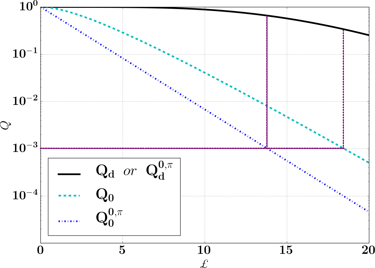
Figure 1: Variation of FAP and DP of $\mathcal{L}$ and $\mathcal{L}^{0,\pi}$ with respect to the threshold $\pounds$ for $\bm{\rho}_{s}=4.$ For a fixed FAP of $10^{-3}$, DP of $\mathcal{L}^{0,\pi}$ is $0.67$ while that of $\mathcal{L}$ is $0.35$.

In other words, to achieve the fixed FAP, the threshold for $\mathcal{L}^{0,\pi}$ needs to be lowered than that of $\mathcal{L}$. Therefore more signal events will cross the threshold when the statistic $\mathcal{L}^{0,\pi}$ is used as compared to $\mathcal{L}$. This makes $\mathcal{L}^{0,\pi}$ a better statistic compared to $\mathcal{L}$ in face-on/off case. In Fig.(1), we have plotted FAP and DP of $\mathcal{L}$ and $\mathcal{L}^{0,\pi}$ with respect to the threshold $\pounds$ for $\bm{\rho}_{s}=4.$ For example, when we draw a fixed FAP of $10^{-3}$ line, the figure shows that the DP of $\mathcal{L}^{0,\pi}$ is $0.67$ while that of $\mathcal{L}$ is $0.35$ showing a clear improvement in the DP for $\mathcal{L}^{0,\pi}$.

III.2 Performance of $\mathcal{L}^{0,\pi}$ for an arbitrary inclination angle

In this section, we investigate the performance of $\mathcal{L}^{0,\pi}$ for an incoming signal from a binary with an arbitrary inclination. First, we study the fractional optimum SNR captured by $\mathcal{L}^{0,\pi}$.

We note in the previous section that $\mathcal{L}^{0,\pi}|_{\mathbf{n}=0}=\bm{\rho}_{s}^{2}$ for face-on/off case. However, if we use the same statistic for an arbitrarily oriented binary then, the $\mathbf{z}^{0,\pi}$ would capture a fraction of network matched filter SNR and it would drop with increase in $\epsilon$. We denote this fraction by, $\omega^{0,\pi}\equiv\sqrt{\mathcal{L}^{0,\pi}}/\bm{\rho}_{s}$.

In Appendix-B, we derive the expression for $\omega^{0,\pi}$ and show that for a wide range of $\epsilon$, either $\omega^{0}$ or $\omega^{\pi}$ is close one. Specifically, for $\epsilon\leq 70^{\circ}$, $\omega^{0}\approx 1$ and for $110\leq\epsilon\leq 180^{\circ}$, $\omega^{\pi}\approx 1$. (Please see Appendix-B for details.) This is elaborated in Fig.(2). It shows the behavior of $\omega^{0}$ and $\omega^{\pi}$ with respect to $\epsilon$ for a network LHV, with Ligo-Livingston (L), Ligo- Hanford (H) and Virgo (V) as the constituent detectors. The signal is from a $(2-10~{}M_{\odot})$ NS-BH binary located at $(\theta=140^{\circ},\phi=100^{0})$. We assume fixed multi-detector optimum SNR, $\bm{\rho}_{s}=6$. The plots are drawn for two different values of polarization angle, $\Psi=0^{\circ}$ and $\Psi=45^{\circ}$. We note that for these values, for a fixed $\Psi$, the fraction $\omega^{0,\pi}$ captures most of the SNR for almost all values of $\epsilon$ except a window of $40^{\circ}$ centered at $\epsilon=90^{\circ}$ (edge on case). Please note that the width of this window has small variation with respect to $\Psi$ as shown in the figure.

In Fig.(3), we further elaborate the same by drawing the maps of $\omega^{0}$ and $\omega^{\pi}$ in the $(\epsilon-\psi)$ plane (see panel (a) and (b)). We draw contours of constant $\omega^{0,\pi}$ at values $\omega^{0,\pi}=0.98,0.9,0.8$. It is clear that $\forall~{}\epsilon\leq 70^{\circ}~{}\&~{}\forall~{}\Psi$, $\omega^{o}\geq 0.98$. Similarly, for $110^{\circ}\leq\epsilon\leq 180^{\circ}~{}\&~{}\forall~{}\Psi$, $\omega^{\pi}\geq 0.98$. A small region of parameters with $70^{\circ}<\epsilon<110^{\circ}$ shows poor response to both $\mathbf{z}^{0}$ and $\mathbf{z}^{\pi}$. The $\omega^{0}$ and $\omega^{\pi}$ are minimum at the point $\left(\epsilon=90^{\circ},\chi=45^{\circ}\right)$ (Please note, $\chi=\Psi-\delta/4$ as defined in Sec.II). We expect that the synthetic streams tuned for face-on/off would give poor response to the edge-on binary. Further we note, $\omega^{0}$ and $\omega^{\pi}$ are complimentary in nature about $\epsilon=90^{0}$. In panel (c), we draw the map of $\max\{\omega^{0},\omega^{\pi}\}$. This shows that barring a small region near edge-on, either $\mathbf{z}^{0}$ or $\mathbf{z}^{\pi}$ captures large fraction of $\bm{\rho}_{s}$.

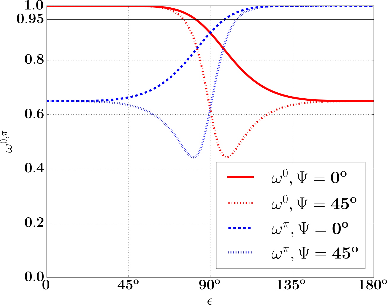
Figure 2: Variation of $\omega^{0}$ and $\omega^{\pi}$ with respect to the inclination angle $\epsilon$ for 2 different values of $\Psi$ in the network LHV. The signal with SNR, $\bm{\rho}_{s}=6$ is from $(2-10M_{\odot})$ NS-BH system optimally located at $(\theta=140^{\circ},\phi=100^{\circ})$. We assume ”zero-detuning, high power” Advanced LIGO PSD for all detectorsaLI (2010).

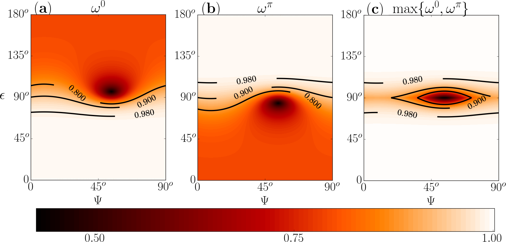
Figure 3: Map of $\omega^{0}$, $\omega^{\pi}$ and $\max\{\omega^{0},\omega^{\pi}\}$ in $(\epsilon,\Psi)$ plane for a network LHV. The signal is from $(2-10M_{\odot})$ NS-BH system optimally located at $(\theta=140^{\circ},\phi=100^{\circ})$. The multi-detector matched filter SNR, $\bm{\rho}_{s}=6$. We assume ”zero-detuning, high power” Advanced LIGO PSDaLI (2010) for all detectors.

In the rest of the section, we comment on the statistical properties of $\mathcal{L}^{0,\pi}$ for an arbitrary inclination. The main difference for an arbitrarily oriented binary from face-on/off case is that $\mathbf{z}^{0,\pi}$ captures a fraction of $\bm{\rho}_{s}$ instead of $\bm{\rho}_{s}$. Thus in presence of signal, the distribution of $\mathcal{L}^{0,\pi}$ for any arbitrary $\epsilon$ is same as Eq.(23) with $\bm{\rho}_{s}$ replaced by $\omega^{0,\pi}\bm{\rho}_{s}$ as given below

$$p_{1}(\mathcal{L}^{0,\pi})=\frac{1}{2}\exp\left[-\frac{\mathcal{L}^{0,\pi}+(\omega^{0,\pi}\bm{\rho}_{s})^{2}}{2}\right]I_{0}\left(\omega^{0,\pi}\bm{\rho}_{s}\sqrt{\mathcal{L}^{0,\pi}}\right).$$ (25)

Further the DP remains the same as Eq. (24), where $\bm{\rho}_{s}$ replaced by $\omega^{0,\pi}\bm{\rho}_{s}$ as given below.

$$Q^{0,\pi}_{d}(\pounds)\approx\frac{1}{2}\textbf{erfc}\left(\frac{\sqrt{\pounds}-\omega^{0,\pi}\bm{\rho}_{s}}{\sqrt{2}}\right).$$ (26)

Since FAP depends only on noise model and construction of statistic, the FAP of $\mathcal{L}^{0,\pi}$ for an arbitrary inclination is same as Eq.(22).

As we discussed earlier, $\mathcal{L}^{0}$ captures more than $98\%$ of $\bm{\rho}_{s}$ for $\epsilon\leq 70^{\circ}$ while $\mathcal{L}^{\pi}$ captures more than $98\%$ of $\bm{\rho}_{s}$ for $\epsilon\geq 110^{\circ}$. Further, the Fig.(3) shows the complimentary behavior of the two statistics $\mathcal{L}^{0}$ and $\mathcal{L}^{\pi}$. In addition, both $\mathcal{L}^{0}$ and $\mathcal{L}^{\pi}$ are constructed out of a single synthetic stream as opposed to the $\mathcal{L}$ statistic (two streams). This motivates us to construct a hybrid statistic out of $\mathcal{L}^{0}$ and $\mathcal{L}^{\pi}$ which would capture most of the multi-detector SNR for a large range of binary inclinations for the CBC search.

IV Proposal of Hybrid Statistic $\mathcal{L}^{mx}$

In this section we propose a hybrid statistic as $\mathcal{L}^{mx}\equiv\max\{\mathcal{L}^{0},\mathcal{L}^{\pi}\}$ and study its statistical properties.

In absence of signal, both $\mathcal{L}^{0}$ and $\mathcal{L}^{\pi}$ follows $\chi^{2}$ distribution with 2 degrees of freedom (see Eq.(21)). Let $\textbf{P}(\mathcal{L}^{0},\mathcal{L}^{\pi})$ be the joint probability distribution of $\mathcal{L}^{0}$ and $\mathcal{L}^{\pi}$ then, the probability distribution of $\mathcal{L}^{mx}$ can be written down as

$$p_{0}(\mathcal{L}^{mx})=2\int_{0}^{\mathcal{L}^{mx}}\textbf{P}(\mathcal{L}^{0}=\mathcal{L}^{mx},\mathcal{L}^{\pi})~{}d\mathcal{L}^{\pi}.$$ (27)

Please note, here $\mathcal{L}^{0}$ and $\mathcal{L}^{\pi}$ have non zero covariance. i.e, they are not independent of each other.

In Eq.(37), $\mathcal{L}^{0,\pi}$ is expressed in terms of $\mathbf{z}_{L,R}$ as,

$$\mathcal{L}^{0,\pi} = \left(\frac{\|\mathbf{F}^{{}^{\prime}}_{+}\|}{\|\mathbf{F}^{{}^{\prime}}\|}~{}\langle\mathbf{z}_{L}|\mathbf{h}_{0}\rangle\pm\frac{\|\mathbf{F}^{{}^{\prime}}_{\times}\|}{\|\mathbf{F}^{{}^{\prime}}\|}~{}\langle\mathbf{z}_{R}|\mathbf{h}_{\pi}/2\rangle\right)^{2}$$ (28)

$$+ \left(\frac{\|\mathbf{F}^{{}^{\prime}}_{+}\|}{\|\mathbf{F}^{{}^{\prime}}\|}~{}\langle\mathbf{z}_{L}|\mathbf{h}_{\pi}/2\rangle\mp\frac{\|\mathbf{F}^{{}^{\prime}}_{\times}\|}{\|\mathbf{F}^{{}^{\prime}}\|}~{}\langle\mathbf{z}_{R}|\mathbf{h}_{0}\rangle\right)^{2}.$$

In absence of signal, each of $\langle\mathbf{z}_{L,R}|\mathbf{h}_{0,\pi}\rangle$ follows independent Gaussian distribution with zero mean and unit variance. This ensures the terms inside the two brackets in Eq.(28) follow Gaussian distribution with zero mean and unit variance. This implies,

$$\mathcal{L}^{0}\equiv n_{1}^{2}+n_{2}^{2},~{}~{}~{}~{}~{}\mathcal{L}^{\pi}\equiv n_{3}^{3}+n_{4}^{2},$$ (29)

such that $n_{1,2,3,4}$ as standard normal variates with

$$\mathrm{Cov}(n_{1},n_{3}) = \mathrm{Cov}(n_{2},n_{4})=\frac{\|\mathbf{F}^{{}^{\prime}}_{+}\|^{2}-\|\mathbf{F}^{{}^{\prime}}_{\times}\|^{2}}{\|\mathbf{F}^{{}^{\prime}}\|^{2}}\equiv c,$$

$$\mathrm{Cov}(n_{1},n_{2}) = \mathrm{Cov}(n_{3},n_{4})=0.$$ (30)

Then the joint distribution of $\sqrt{\mathcal{L}^{0}}$ and $\sqrt{\mathcal{L}^{\pi}}$ is a 2-dimensional generalized Rayleigh distribution and is given by Eq.(2.1) of Blumenson and Miller (1963) as,

$$\textbf{P}(\sqrt{\mathcal{L}^{0}},\sqrt{\mathcal{L}^{\pi}})= \frac{\sqrt{\mathcal{L}^{0}\mathcal{L}^{\pi}}}{c}~{}e^{-\frac{\mathcal{L}^{0}+\mathcal{L}^{\pi}}{2\left(1-c^{2}\right)}}$$ (31)

$$I_{0}\left(\frac{c}{1-c^{2}}\sqrt{\mathcal{L}^{0}\mathcal{L}^{\pi}}\right).$$

This implies,

$$\textbf{P}(\mathcal{L}^{0},\mathcal{L}^{\pi}) = \frac{1}{4\sqrt{\mathcal{L}^{0}\mathcal{L}^{\pi}}}\textbf{P}(\sqrt{\mathcal{L}^{0}},\sqrt{Lc^{\pi}})$$ (32)

$$= \frac{1}{4~{}c}~{}e^{-\frac{\mathcal{L}^{0}+\mathcal{L}^{\pi}}{2\left(1-c^{2}\right)}}~{}I_{0}\left(\frac{c}{1-c^{2}}\sqrt{\mathcal{L}^{0}\mathcal{L}^{\pi}}\right).$$

Substitution of Eq.(32) in Eq.(27) gives the distribution of $\mathcal{L}^{mx}$ in absence of signal as,

$$p_{0}(\mathcal{L}^{mx} ) =\frac{1}{2~{}c}~{}e^{-\frac{\mathcal{L}^{mx}}{2\left(1-c^{2}\right)}}$$ (33)

$$\int_{0}^{\mathcal{L}^{mx}}e^{-\frac{\mathcal{L}^{\pi}}{2\left(1-c^{2}\right)}}~{}I_{0}\left(\frac{c}{1-c^{2}}\sqrt{\mathcal{L}^{mx}\mathcal{L}^{\pi}}\right)~{}d\mathcal{L}^{\pi}.$$

In presence of signal, for high multi-detector matched filter SNR $\bm{\rho}_{s}$, as discussed in Sec.III.2, the distribution of $\sqrt{\mathcal{L}^{0,\pi}}$ can be approximated by Gaussian distribution with mean $\omega^{0,\pi}\bm{\rho}_{s}$ and unit variance. But for high $\bm{\rho}_{s}$, $\mathcal{L}^{mx}=\mathcal{L}^{0}$ in the region $0^{\circ}\leq\epsilon\leq 70^{\circ}$ and $\mathcal{L}^{mx}=\mathcal{L}^{\pi}$ in the region $110^{\circ}\leq\epsilon\leq 180^{\circ}$. Thus the distribution of $\mathcal{L}^{mx}$ in the presence of signal can be approximated as,

$$p_{1}(\mathcal{L}^{mx})\approx\begin{cases}p_{1}(\mathcal{L}^{0}),&0\leq\epsilon<70^{\circ},\\ p_{1}(\mathcal{L}^{\pi}),&110^{\circ}<\epsilon\leq 180^{\circ}\,.\end{cases}$$

The FAP and DP of $\mathcal{L}^{mx}$ can be obtained by numerically integrating $p_{0}(\mathcal{L}^{mx})$ and $p_{1}(\mathcal{L}^{mx})$.

In the next section, we carry out numerical simulations to study the statistical properties of $\mathcal{L},\mathcal{L}^{0,\pi}$ and the hybrid statistic $\mathcal{L}^{mx}$. Further, we study the performance of all 4 statistics in terms of the Receiver Operator Characteristic (ROC) curve for various signal configurations.

V Simulations and Discussion

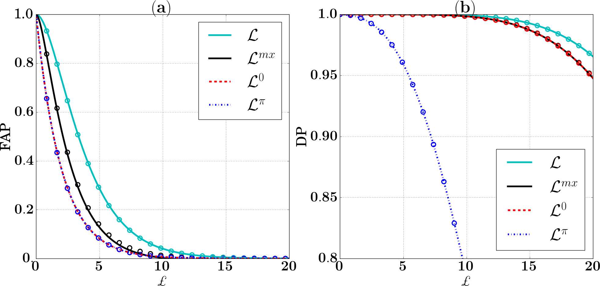
(a)

Figure 4: (a) Variation in FAP of different statistics with respect to the threshold $\pounds$. (b) Variation in DP of different statistics with respect to the threshold $\pounds$ for signal from $(2-10M_{\odot})$ non spinning NS-BH binary system with $\bm{\rho}_{s}=6$ optimally located at $(\theta=140^{\circ},\phi=100^{\circ})$ with arbitrary $\epsilon=45^{\circ}$ and $\Psi=45^{\circ}$. The curves are generated from the theory and circles are from simulations. We assume ”zero-detuning, high power” Advanced LIGO PSDaLI (2010) for all detectors.

In this section, we carry out numerical simulations for a three detector network LHV. All the detectors are assumed to have Gaussian, random noise with the noise PSD following ”zero-detuning, high power” Advanced LIGO noise curveaLI (2010). The GW signal from non spinning NS-BH ($2-10~{}M_{\odot}$) binary system is injected with SNR $\bm{\rho}_{s}=6$. We assume that the masses are fixed and known for this comparison study. Of course, in real situation, the masses are unknown and then one needs to place templates in mass space and perform the search. We know that a template based search increases the false alarms. However, this applies to the search based on both hybrid statistic, $\mathcal{L}^{mx}$ and the MLR statistic, $\mathcal{L}$ and further owing to a single stream, we expect to get less false alarms for hybrid statistic as compared to the MLR statistic. As mentioned in Sec.I, based on simple arguments in gravitational wave follow-up of short Gamma Ray Bursts of IPN triggers, in Williamson et al. (2014) authors used a face on/off tuned MLR statistic (single stream) for nearly on-axis GRBs. This was targeted search with templates in mass parameter space in LIGO-Virgo data. They did show a similar improvement in the false alarm rates compared to generic MLR statistic as we got in the fixed masses simulations of hybrid described below.

The simulation results are as follows. First we compare the theoretical and numerically evaluated FAP and DP for all the 4 statistics $\mathcal{L}$, $\mathcal{L}^{mx}$, $\mathcal{L}^{0}$ and $\mathcal{L}^{\pi}$ and then the performance of the hybrid statistic is compared with the generic MLR statistic, $\mathcal{L}$. This performance is quantified by drawing the ROC plots, i.e, the plot between FAP and DP. In all the plots, The $\mathcal{L}$ statistic is represented by cyan(solid) line, $\mathcal{L}^{mx}$ by black(solid) line, $\mathcal{L}^{0}$ by red(dash) line and $\mathcal{L}^{\pi}$ by blue(dash-dot) line.

V.1 Comparison of analytical and numerical FAP and DP

In Sec.IV, we obtain the analytical expression for distributions, of $\mathcal{L}^{mx}$ in presence and absence of signal i.e. $p_{0}(\mathcal{L}^{mx})$ and $p_{1}(\mathcal{L}^{mx})$. Theoretical FAP and DP for different thresholds is computed by integrating $p_{0,1}(\mathcal{L}^{mx})$. Here, we compare the theoretical FAP and DP with those obtained by numerical simulations.

We generate the network data with $2\times 10^{6}$ noise realizations with a fixed signal from NS-BH system located at $(\theta=140^{\circ},\phi=100^{\circ})$ (one of the best location for LHV network based on the joint antenna power response) with $\epsilon=\psi=45^{\circ}$. For each noise realization, all the four $\mathcal{L}$, $\mathcal{L}^{mx}$, $\mathcal{L}^{0}$, $\mathcal{L}^{\pi}$ statistics are computed. For a given threshold $\pounds$, we count the number of times each of the statistics crosses the threshold value when the data contains only the noise (gives FAP) as well as when the data contains signal plus noise (gives DP).

In Fig.(4), panel (a) represents the FAP vs $\pounds$ for all the 4 statistics. The open circles denote FAP computed through simulations as detailed above whereas the continuous lines denote the theoretically obtained FAP. We observe a remarkable agreement of the analytical result with the numerical simulation. The main result derived and understood from panel (a) of Fig.(4), is the difference in the FAP values corresponding to a given threshold for various statistic. Owing to two data streams, $\mathcal{L}$ gives the maximum FAP amongst all the four. Since $\mathcal{L}^{0,\pi}$ are constructed out of a single synthetic stream, the FAP of both is identical as well as the least amongst the four. Since the hybrid statistic is constructed out $\mathcal{L}^{0,\pi}$, its FAP is slightly higher than that of $\mathcal{L}^{0,\pi}$.

The panel (b) of Fig.(4), represents the DP vs $\pounds$ for all the 4 statistics. The open circles denote the DP from simulations whereas the continuous lines denote the theoretical DP. Since the DP for all the 4 statistics depends on the fractional optimal SNR captured by the individual statistic, the DP of $\mathcal{L}$ is maximum as it captures $\bm{\rho}_{s}$ in no noise case. For the signal with $\epsilon=45^{\circ}$, $\mathcal{L}^{mx}$ is $\mathcal{L}^{0}$ most of the time, thus the DP of $\mathcal{L}^{mx}$ and $\mathcal{L}^{0}$ overlap. The statistic $\mathcal{L}^{\pi}$ captures a small fraction of the $\bm{\rho}_{s}$ (see Fig.(3)) and hence shows the least DP. Once again, we see remarkable agreement of numerically computed DP with the analytically integrated DP for all the statistics.

V.2 Performance of hybrid statistic for a single injection

In this subsection, we study the performance of $\mathcal{L}^{mx}$ against rest of the statistics, more importantly the generic multi-detector MLR statistic $\mathcal{L}$.

We generate the network data with $2\times 10^{6}$ noise realizations and a fixed signal from NS-BH system optimally located at $(\theta=140^{\circ},\phi=100^{\circ})$ with an arbitrary $\psi=45^{\circ}$ but varying binary inclination. We select 6 binary inclination angles namely $\epsilon=0^{\circ},45^{\circ},70^{\circ},90^{\circ},135^{\circ},180^{\circ}$ and obtain the ROC curve numerically as shown in panels (a), (b), (c), (d), (e), (f) of Fig.(5) respectively. We summarize the results as below.

For $\epsilon=0~{}OR~{}\pi$ case, $\mathcal{L}^{mx}$ (being optimized for the face-on/off case) is expected to perform better than the generic MLR statistic. Panel (a) and (e) shows the same. As discussed earlier, this improvement is primarily due to the reduction in the FAP of $\mathcal{L}^{mx}$. For a fixed FAP of $10^{-5}$, the subsequent improvement in the DP is $6\%$ which translates in an increase in the detection rate of $6\%$.

For $\epsilon=45^{\circ}~{}OR~{}135^{\circ}$ case, (symmetrical located from $0$ and $\pi$ cases respectively) as seen in panel (b) and (e), the improvement in ROC of $\mathcal{L}^{mx}$ compared to that of $\mathcal{L}$ is similar. This improvement is due to the drop in FAP of $\mathcal{L}^{mx}$. As shown in Appendix-B, at $\epsilon=45^{\circ}$, the $\mathcal{L}^{mx}$ captures all the optimum SNR. Thus the improvement in DP remains close to $6\%$ similar to the face-on/off case.

Following the above argument, as $\epsilon$ approaches the edge-on case, the fractional SNR captured in $\mathcal{L}^{mx}$ reduces. Thus ROC of $\mathcal{L}^{mx}$ starts approaching that of ROC of $\mathcal{L}$ as seen in panel (c). Here, the improvement of $\mathcal{L}^{mx}$ is $2\%$ over the $\mathcal{L}$.

For $\epsilon=90^{\circ}$ case, the fractional optimal SNR captured by $\mathcal{L}^{mx}$ is very small as $\mathcal{L}^{mx}$ is optimized for face-on/off case. Thus, the MLR statistic performs better than the $\mathcal{L}^{mx}$ at the edge-on case as shown in panel (d) of Fig.(3).

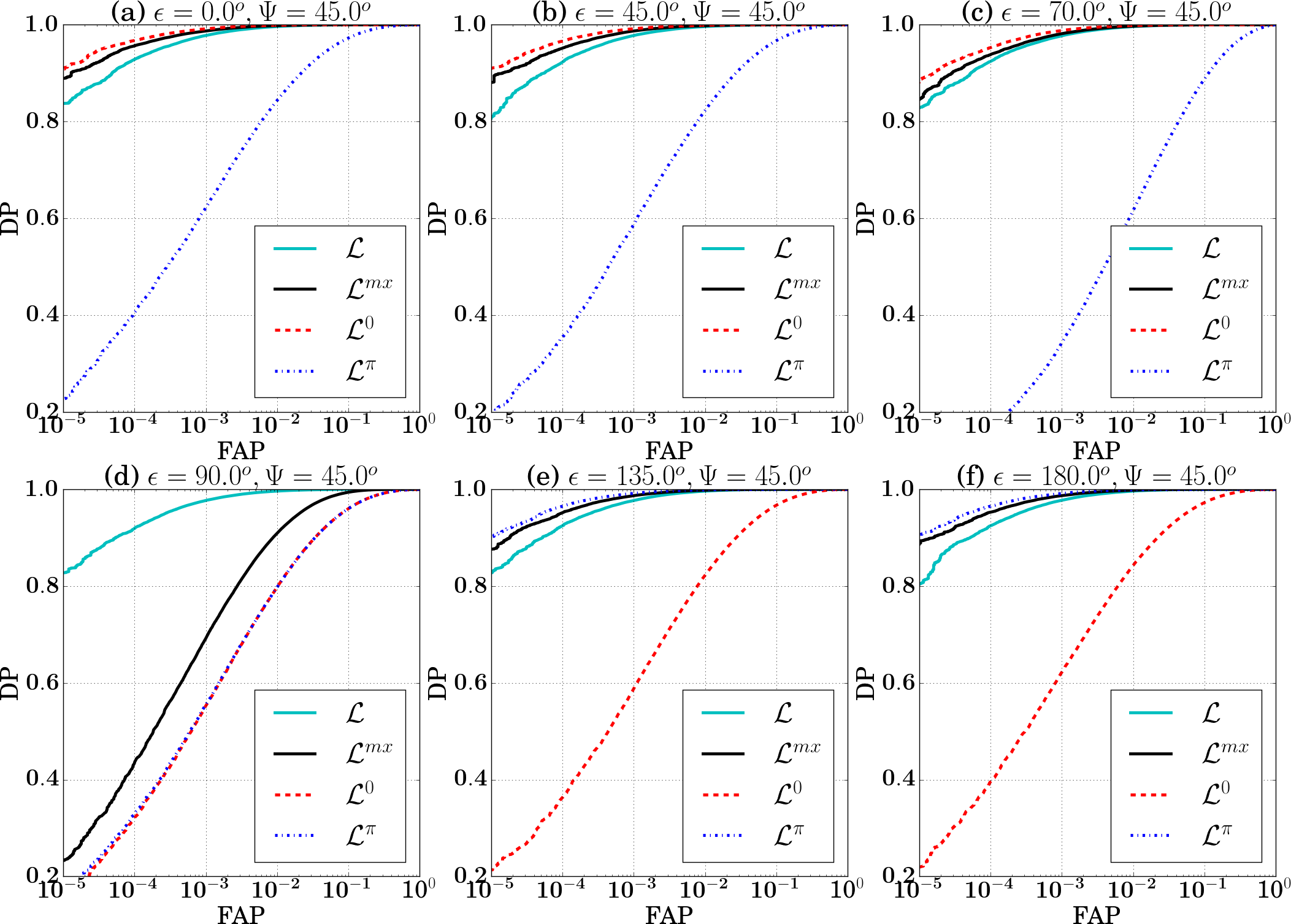
(a)

Figure 5: ROC plots of the 4 statistics corresponding to a network LHV for fixed injections with different values of $\epsilon$. The signal with SNR, $\bm{\rho}_{s}=6$ is from $(2-10M_{\odot})$ NS-BH system optimally located at $(\theta=140^{\circ},\phi=100^{\circ})$ with an arbitrary polarization angle $\psi=45^{\circ}$. We assume ”zero-detuning, high power” Advanced LIGO PSDaLI (2010) for all detectors.

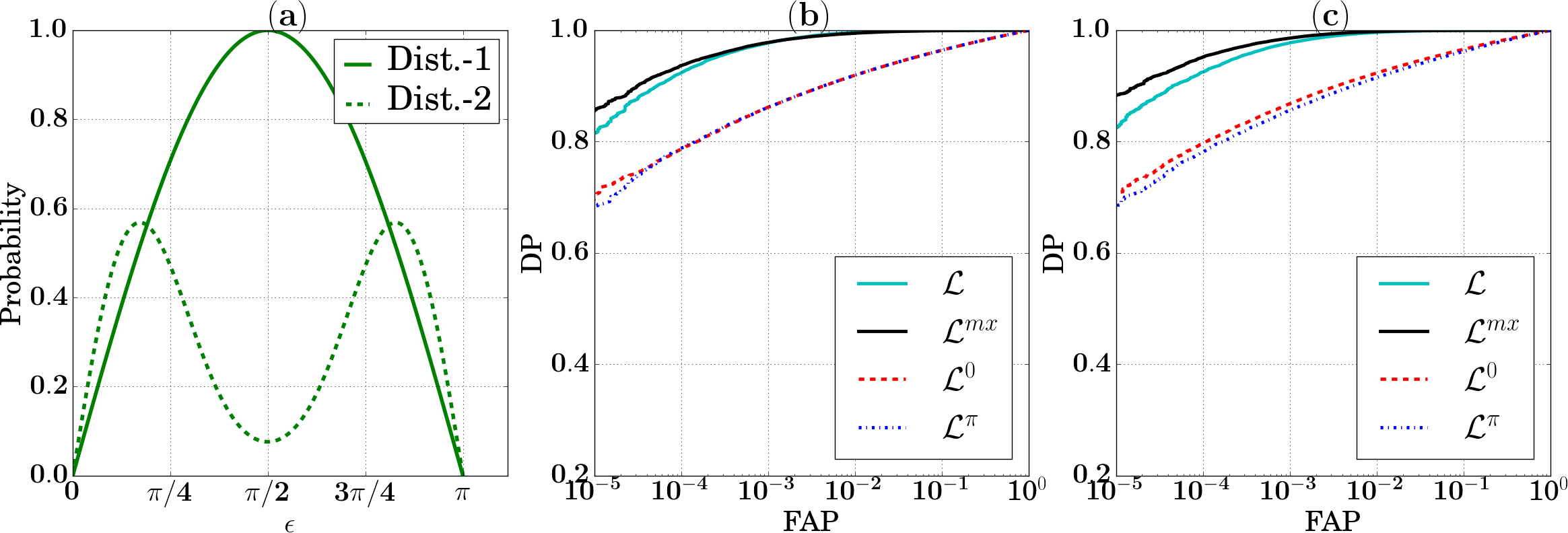
(a)

Figure 6: Panel (a) is the plot of two sampling distributions of $\epsilon$. Panel (b) gives ROC plots for 4 different statistics corresponding to a network LHV when the injected signal’s inclination angle, $\epsilon$ drawn from Dist-1 and panel (c) gives ROC plots for injections with $\epsilon$ drawn from Dist-2. In both cases sky location, and polarization angle are sampled uniformly. The injections are with SNR, $\bm{\rho}_{s}=6$ and are from $(2-10M_{\odot})$ NS-BH system. We assume ”zero-detuning, high power” Advanced LIGO PSDaLI (2010) for all detectors.

V.3 Performance of the hybrid statistic for injections sampled from a distribution

In this simulation, we generate the network data with $2\times 10^{6}$ noise realizations and signals from NS-BH system with masses $(2-10M_{\odot})$ and multi-detector SNR $\rho_{s}=6$. We randomly draw the binary inclination angle $\epsilon$, polarization angle $\Psi$ and source location $(\theta,\phi)$ from a given distribution. We perform this exercise for two distinct distributions, Dist-1 and Dist-2 of inclination angle $\epsilon$. In both cases, $\cos\theta$, $\phi$ and $\Psi$ are sampled uniformly from the intervals $[-1,1]$, $[0^{\circ},360^{\circ}]$ and $[0^{\circ},90^{\circ}]$ respectively.

The Dist-1, draws $\cos(\epsilon)$ uniformly from [-1,1] and is denoted by a green (solid) line in panel (a) of Fig.(6). As seen, in the figure, the population of random samples drawn from this distribution contains more of edge-on sources than that of face-on.

In Dist-2, the $\epsilon$ follows the distribution proposed in Eq.(28) of Schutz (2011) [see green (dashed) line in panel (a) of Fig.(6)].

$$\textbf{P}(\epsilon)=0.076076\left(1+6\cos^{2}\epsilon+\cos^{4}\epsilon\right)^{3/2}\sin\epsilon.$$ (34)

The Dist-2 is a realistic distribution of $\epsilon$, where the SNR information is folded in the distribution along with the geometric prior. Since we know that the edge-on sources have less SNR than face-on sources, we expect to see less number of edge-on systems than face-on. As a result, there would be a dip in the curve (dashed line) with respect to the Dist -1 (solid line).

In Fig.(6), panels (b) and (c) summarize the results in terms of the ROC curves using Dist -1 and Dist -2 respectively. The ROC curve summarizes the performance of MLR statistic compared to the hybrid statistic averaged over all the source locations and the polarizations.

Panel (b) shows that for Dist -1, the average performance of $\mathcal{L}^{mx}$ is better than that of $\mathcal{L}$ in spite of more number of sources located around edge-on. Quantitatively, DP improves by $\sim 5\%$ for FAP $10^{-5}$.

However, panel (c) shows more realistic performance as we expect the inclination angle distribution to be more realistic in this case. We note that for Dist - 2, the hybrid statistic performs much better than the MLR statistic $\mathcal{L}$. Quantitatively, for an FAP of $10^{-5}$, $\mathcal{L}^{mx}$ improves the DP by $~{}7\%$ over $\mathcal{L}$.

V.4 Conclusion and future directions

In this article, we revisit the problem CBC GW search with a multi-detector network with advanced interferometers like LIGO-Virgo in coherent approach. We show that the hybrid statistic constructed from two statistics namely; coherent MLR statistic tuned for face-on and face-off binaries captures most of multi-detector optimum SNR for a large fraction of the binary inclination angles except a small window centered around the edge-on case. The statistical properties of this hybrid statistic is studied in detail. The performance of this hybrid statistic is compared with that of the coherent MLR statistic for generic inclination angles. Being constructed from the single synthetic data stream, the hybrid statistic gives low false alarms compared to the two streams generic multi-detector MLR statistic and very small fractional loss in the optimum SNR for a large range of binary inclinations.

We have demonstrated the performance by using the noise model as Gaussian with ”zero-detuning, high power” Advanced LIGO PSDaLI (2010) in LHV network for the NS-BH system of masses ($2-10M_{\odot}$) for a fixed SNR of 6. The ROC curves are used as a tool for this demonstration. The simulations are performed for two cases.

Case 1: The source is optimally located in the LHV network and oriented with various binary inclination angles. The ROC curves show the hybrid statistic performs better than the generic MLR statistic for all the inclination angles less then $70^{\circ}$ and greater than $110^{\circ}$. The improvement in each of them corresponds to two factors. First, the hybrid statistic captures most of the optimum SNR for a large region of inclination and polarization parameter space. Thus, we do not loose much in the DP for a given multi-detector matched filter SNR $\bm{\rho}_{s}$. Further, by construction the hybrid statistic is out of a single stream. Thus, the FAP of the hybrid statistic is better than that of the two stream generic MLR statistic (of course it is slightly worst than the pure single streams $\mathcal{L}^{0}$ and $\mathcal{L}^{\pi}$ ).

Case 2: The source location as well as the orientation and polarization are sampled from a distribution. The source location is sampled uniformly from the sky sphere. The polarization angle follows a uniform distribution. The inclination angles are drawn from two distributions namely $U[\cos(\epsilon)]$ and more realistic distribution proposed in Schutz (2011) . The ROC curve shows that the performance of hybrid statistic gives an improvement of $\sim 5\%$ and $\sim 7\%$ respectively in DP compared to the generic multi-detector MLR statistic for a fixed FAP of $10^{-5}$.

In Williamson et al. (2014), authors applied a similar statistic for the SGRB follow-up search for very small inclination angles. However, this study and its performance in Gaussian noise clearly shows that the ${\it hybrid}$ statistic would give better performance for wide range of inclination angles barring a small window around the edge-on case. Since, we expect that the source population would have bias towards the face-on/off cases due to the relative difference in the SNRs, this statistic would play a crucial role in the multi-detector CBC search in the advanced era.

We plan to apply this for the S6 noise of the science run of LIGO detectors and test the performance of the statistic for generic inclination angles. We also plan to extend the study for a larger network, which includes LIGO-India and KAGRA.

VI Acknowledgment

The authors availed the 128 cores computing facility established by the MPG-DST Max Planck Partner Group at IISER TVM. The authors would like to thank S. Fairhurst for reviewing the draft and for useful comments. This document has been assigned LIGO laboratory document number LIGO-P1500221.

Appendix A Relation between $\{\text{A},\phi_{a},\epsilon,\Psi\}$ and $\{\bm{\rho}_{L},\bm{\rho}_{R},\Phi_{L},\Phi_{R}\}$

The new parameters, $\{\bm{\rho}_{L},\bm{\rho}_{R},\Phi_{L},\Phi_{R}\}$ are related to the physical parameters, $\{\text{A},\phi_{a},\epsilon,\Psi\}$ as below,

$$\bm{\rho}_{L}e^{i\Phi_{L}} = \text{A}\|\mathbf{F}_{+}^{{}^{\prime}}\|e^{i\phi_{a}}\left[\frac{1+\cos^{2}\epsilon}{2}\cos 2\chi+i\cos\epsilon\sin 2\chi\right],$$

$$\bm{\rho}_{R}e^{i\Phi_{R}} = \text{A}\|\mathbf{F}_{\times}^{{}^{\prime}}\|e^{i\phi_{a}}\left[\frac{1+\cos^{2}\epsilon}{2}\sin 2\chi-i\cos\epsilon\cos 2\chi\right].$$

The absolute values and the phases of the above equations are $\{\bm{\rho}_{L},\bm{\rho}_{R},\Phi_{L},\Phi_{R}\}$ and explicitly given in Eq.(B1) of Haris and Pai (2014).

Appendix B $\mathcal{L}^{0,\pi}$ in absence of noise

In this section we derive the expression for fraction of multi-detector matched filter SNR captured by the statistics, $\mathcal{L}^{0}$ and $\mathcal{L}^{\pi}$.

From Eq.(5) and Eq.(18), $\mathbf{z}^{0,\pi}$ can be re-expressed in terms of $\mathbf{z}_{L,R}$ as below.

$$\tilde{\tilde{z}}^{0,\pi}(f)=\frac{\|\mathbf{F}^{{}^{\prime}}_{+}\|}{\|\mathbf{F}^{{}^{\prime}}\|}~{}\tilde{\tilde{z}}_{L}(f)\pm i\frac{\|\mathbf{F}^{{}^{\prime}}_{\times}\|}{\|\mathbf{F}^{{}^{\prime}}\|}~{}\tilde{\tilde{z}}_{R}(f),$$ (36)

where $(+)$ corresponds to $\mathbf{z}^{0}$ and $(-)$ corresponds to $\mathbf{z}^{\pi}$. By substituting back in Eq.(19), $\mathcal{L}^{0,\pi}$ can be expanded in terms of the four terms $\langle\mathbf{z}_{L,R}|\mathbf{h}_{0,\pi}\rangle$.

$$\mathcal{L}^{0,\pi} = \left(\frac{\|\mathbf{F}^{{}^{\prime}}_{+}\|}{\|\mathbf{F}^{{}^{\prime}}\|}~{}\langle\mathbf{z}_{L}|\mathbf{h}_{0}\rangle\pm\frac{\|\mathbf{F}^{{}^{\prime}}_{\times}\|}{\|\mathbf{F}^{{}^{\prime}}\|}~{}\langle\mathbf{z}_{R}|\mathbf{h}_{\pi/2}\rangle\right)^{2}$$ (37)

$$+ \left(\frac{\|\mathbf{F}^{{}^{\prime}}_{+}\|}{\|\mathbf{F}^{{}^{\prime}}\|}~{}\langle\mathbf{z}_{L}|\mathbf{h}_{\pi/2}\rangle\mp\frac{\|\mathbf{F}^{{}^{\prime}}_{\times}\|}{\|\mathbf{F}^{{}^{\prime}}\|}~{}\langle\mathbf{z}_{R}|\mathbf{h}_{0}\rangle\right)^{2}.$$

Using Eq.(1) and Eq.(LABEL:parametrs), the scalar products in the above equation in the absence of noise can be written as,

$$\langle\mathbf{z}_{L}|\mathbf{h}_{0}\rangle|_{\mathbf{n}=0}=\Re\left[\bm{\rho}_{L}e^{i\Phi_{L}}\right] \,, \langle\mathbf{z}_{L}|\mathbf{h}_{\pi/2}\rangle|_{\mathbf{n}=0}=-\Im\left[\bm{\rho}_{L}e^{i\Phi_{L}}\right],$$

$$\langle\mathbf{z}_{R}|\mathbf{h}_{0}\rangle|_{\mathbf{n}=0}=\Re\left[\bm{\rho}_{R}e^{i\Phi_{R}}\right] \,, \langle\mathbf{z}_{R}|\mathbf{h}_{\pi/2}\rangle|_{\mathbf{n}=0}=-\Im\left[\bm{\rho}_{R}e^{i\Phi_{R}}\right].$$

Substituting in Eq.(37) give,

$$\mathcal{L}^{0,\pi}|_{\mathbf{n}=0}=\left|\frac{\|\mathbf{F}^{{}^{\prime}}_{+}\|}{\|\mathbf{F}^{{}^{\prime}}\|}~{}\bm{\rho}_{Ls}~{}e^{i\Phi_{Ls}}\pm i~{}~{}\frac{\|\mathbf{F}^{{}^{\prime}}_{\times}\|}{\|\mathbf{F}^{{}^{\prime}}\|}~{}\bm{\rho}_{Rs}~{}e^{i\Phi_{Rs}}\right|^{2}.$$ (39)

We further expand Eq.(39) in terms of the physical parameters to obtain the explicite dependence on $\epsilon$ for fixed SNR case.

$$\mathcal{L}^{0,\pi}|_{\mathbf{n}=0} = \frac{\text{A}^{2}}{\|\mathbf{F}^{{}^{\prime}}\|^{2}}\left|\|\mathbf{F}^{{}^{\prime}}_{+}\|^{2}\left(\frac{1+\cos^{2}\epsilon}{2}\cos 2\chi+i\cos\epsilon\sin 2\chi\right)\pm~{}i\|\mathbf{F}^{{}^{\prime}}_{\times}\|^{2}\left(\frac{1+\cos^{2}\epsilon}{2}\sin 2\chi-i\cos\epsilon\cos 2\chi\right)\right|^{2}$$ (40)

$$= \frac{\text{A}^{2}}{\|\mathbf{F}^{{}^{\prime}}\|^{2}}\left[\text{T}_{1}~{}\left(\frac{1+\cos^{2}\epsilon}{2}\right)^{2}+\text{T}_{2}~{}\cos^{2}\epsilon\pm\text{T}_{3}~{}\frac{1+\cos^{2}\epsilon}{2}\cos\epsilon\right]~{},$$

where the three terms $T_{1},T_{2},T_{3}$ are defined as below.

$$\text{T}_{1} \equiv \|\mathbf{F}^{{}^{\prime}}_{+}\|^{4}\cos^{2}2\chi+\|\mathbf{F}^{{}^{\prime}}_{\times}\|^{4}\sin^{2}2\chi,$$

$$\text{T}_{2} \equiv \|\mathbf{F}^{{}^{\prime}}_{+}\|^{4}\sin^{2}2\chi+\|\mathbf{F}^{{}^{\prime}}_{\times}\|^{4}\cos^{2}2\chi,$$

$$\text{T}_{3} \equiv 2\|\mathbf{F}^{{}^{\prime}}_{+}\|^{2}\|\mathbf{F}^{{}^{\prime}}_{\times}\|^{2}~{}.$$ (41)

To obtain a fixed multi-detector matched filter SNR $\bm{\rho}_{s}$, face-one binaries should be kept at larger distance than the edge-on binaries. This is because, the face-on binaries carry more polarization power than the edge-on. This reflects in the derived amplitude, A in Eq.(40) as below,

$$\text{A}^{2}=\frac{\bm{\rho}_{s}^{2}}{\text{R}_{1}\left(\frac{1+\cos^{2}\epsilon}{2}\right)^{2}+\text{R}_{2}\cos^{2}\epsilon},$$ (42)

with

$$\text{R}_{1} = \|\mathbf{F}^{{}^{\prime}}_{+}\|^{2}\cos^{2}2\chi+\|\mathbf{F}^{{}^{\prime}}_{\times}\|^{2}\sin^{2}2\chi,$$

$$\text{R}_{2} = \|\mathbf{F}^{{}^{\prime}}_{+}\|^{2}\sin^{2}2\chi+\|\mathbf{F}^{{}^{\prime}}_{\times}\|^{2}\cos^{2}2\chi~{}.$$ (43)

Substitution of Eq.(42) in Eq.(40) gives the fraction, $\omega^{0,\pi}$ of $\bm{\rho}_{s}$ captured by $\mathcal{L}^{0,\pi}$ statistic in the absence of noise.

$$(\omega^{0,\pi})^{2} \equiv \frac{\mathcal{L}^{0,\pi}|_{\mathbf{n}=0}}{\bm{\rho}^{2}_{s}}$$

$$= \frac{\text{T}_{1}~{}\left(\frac{1+\cos^{2}\epsilon}{2}\right)^{2}+\text{T}_{2}~{}\cos^{2}\epsilon\pm\text{T}_{3}~{}\frac{1+\cos^{2}\epsilon}{2}\cos\epsilon}{{\|\mathbf{F}^{\prime}\|^{2}}\left[\text{R}_{1}\left(\frac{1+\cos^{2}\epsilon}{2}\right)^{2}+\text{R}_{2}\cos^{2}\epsilon\right]}.$$

Please note that for the face-on/off case, $\omega^{0,\pi}=1$. However, as we seen in Fig.(3), the $\omega^{0}$ to drop as the signal $\epsilon$ increases from 0 and similarly, we expect $\omega^{\pi}$ to drop as the signal $\epsilon$ drops from $\pi$.

In Eq.(LABEL:Eq-Rho_0Pi-4), the inclination angle $\epsilon$ appear in terms of $\cos\epsilon$ and $\frac{1+\cos^{2}\epsilon}{2}$. If we expand $\cos\epsilon$ about $\epsilon=0$ up to fourth order, then

$$\cos\epsilon \approx 1-\frac{\epsilon^{2}}{2}+\frac{\epsilon^{4}}{24}\equiv\text{Ce},$$

$$\frac{1+\cos^{2}\epsilon}{2} \approx 1-\frac{\epsilon^{2}}{2}+\frac{4\epsilon^{4}}{24}.$$ (45)

Substitution of Eq.(45) in the expression for $\omega^{0}$ gives,

$$(\omega^{0})^{2} = \left.\left(1+\frac{\text{T}_{1}+\text{T}_{3}/2}{4~{}\|\mathbf{F}^{{}^{\prime}}\|^{4}~{}\text{Ce}}~{}\epsilon^{4}\right)\right/\left(1+\frac{\text{R}_{1}}{4~{}\|\mathbf{F}^{{}^{\prime}}\|^{2}~{}\text{Ce}}~{}\epsilon^{4}\right)$$ (46)

$$\approx \left(1+\frac{\text{T}_{1}+\text{T}_{3}/2}{4~{}\|\mathbf{F}^{{}^{\prime}}\|^{4}~{}\text{Ce}}~{}\epsilon^{4}\right)\left(1-\frac{\text{R}_{1}}{4~{}\|\mathbf{F}^{{}^{\prime}}\|^{2}~{}\text{Ce}}~{}\epsilon^{4}\right)$$

$$\approx 1+\frac{\epsilon^{4}}{\text{Ce}~{}\|\mathbf{F}^{\prime}\|^{4}}\left(\text{T}_{1}+\text{T}_{3}/2-\|\mathbf{F}^{\prime}\|^{2}\text{R}_{1}\right),$$

Here we make use of the identities, $\text{T}_{1}+\text{T}_{2}+\text{T}_{3}=\|\mathbf{F}^{\prime}\|^{4}$ and $\text{R}_{1}+\text{R}_{2}=\|\mathbf{F}^{\prime}\|^{2}$ from Eq.(41) and Eq.(43). Again from Eq.(41) and Eq.(43),

$$\text{T}_{1}+\text{T}_{3}/2-\|\mathbf{F}^{\prime}\|^{2}\text{R}_{1}=0.$$ (47)

This implies,

$$\omega^{0}=1.$$ (48)

The $4^{th}$ order approximation of $\cos\epsilon$ given in Eq.(45) is valid for a wide range of $\epsilon$. For $\epsilon\leq 70^{\circ}$, the error in this approximation is less than $1.5\%$. Thus we can safely assume $\omega^{0}\approx 1$ for $0^{\circ}\leq\epsilon\leq 70^{\circ}$. For example, Table 1 gives the minimum values of $\omega^{o}$ over $\Psi$ for various $\epsilon$ in a network LHV for signal from $(2-10M_{\odot})$ NS-BH system located at $(\theta=140^{\circ},\phi=100^{\circ})$.

Binary Inclination, $\epsilon$	$50^{\circ}$	$60^{\circ}$	$70^{\circ}$	$80^{\circ}$
Minimum value of $\omega^{0}$	$0.999$	$0.995$	$0.98$	$0.87$

Table 1: Minimum value of $\omega^{o}$ over $\Psi$ for various $\epsilon$ in a network LHV. The signal is from $(2-10M_{\odot})$ NS-BH system located at $(\theta=140^{\circ},\phi=100^{\circ})$. We assume ”zero-detuning, high power” Advanced LIGO PSDaLI (2010) for all detectors.

Similarly, by expanding $\cos\epsilon$ about $\pi$, it can be easily shown that for $110^{\circ}\leq\epsilon\leq 180^{\circ}$, $\omega^{\pi}\approx 1$. Fig.(2) and Fig.(3) justifies the above claim.

For edge-on binaries, at $\chi=45^{\circ}$ (Please note, $\chi=\Psi-\delta/4$ as defined in Sec.II), from Eq.(LABEL:Eq-Rho_0Pi-4) the SNR fraction captured by $\mathcal{L}^{0,\pi}$ becomes,

$$\omega^{0,\pi}=\frac{\|\mathbf{F}_{\times}^{\prime}\|}{\|\mathbf{F}^{\prime}\|}.$$ (49)

In other words, at this point $\bm{\rho}_{L}$ vanishes and whole network SNR is accumulated in SNR, $\bm{\rho}_{R}$ of sub-dominant stream $\mathbf{z}_{R}$. Since by construction of dominant polarization frame, $\|\mathbf{F}_{\times}^{\prime}\|$ is less than $\|\mathbf{F}_{+}^{\prime}\|$, this result in a minimum $\omega^{0,\pi}$.

References

- Schutz (2011) B. F. Schutz, Classical and Quantum Gravity 28, 125023 (2011), URL http://stacks.iop.org/0264-9381/28/i=12/a=125023.
- Collaboration et al. (2015) T. L. S. Collaboration, J. Aasi, B. P. Abbott, R. Abbott, T. Abbott, M. R. Abernathy, K. Ackley, C. Adams, T. Adams, P. Addesso, et al., Classical and Quantum Gravity 32, 074001 (2015), URL http://stacks.iop.org/0264-9381/32/i=7/a=074001.
- Harry (2010) G. M. Harry (LIGO Scientific), Class. Quant. Grav. 27, 084006 (2010), URL http://stacks.iop.org/0264-9381/27/i=8/a=084006.
- Abbott et al. (2016) B. P. Abbott, R. Abbott, T. D. Abbott, M. R. Abernathy, F. Acernese, K. Ackley, C. Adams, T. Adams, P. Addesso, R. X. Adhikari, et al. (LIGO Scientific Collaboration and Virgo Collaboration), Phys. Rev. Lett. 116, 061102 (2016), URL http://link.aps.org/doi/10.1103/PhysRevLett.116.061102.
- Acernese et al. (2015) F. Acernese et al. (VIRGO), Class. Quant. Grav. 32, 024001 (2015), eprint 1408.3978, URL http://stacks.iop.org/0264-9381/32/i=2/a=024001.
- The Virgo Collaboration (2012) The Virgo Collaboration, Tech. Rep. VIR-0128A-12, Virgo Collaboration (2012), URL https://tds.ego-gw.it/ql/?c=8940.
- Aso et al. (2013) Y. Aso, Y. Michimura, K. Somiya, M. Ando, O. Miyakawa, T. Sekiguchi, D. Tatsumi, and H. Yamamoto (The KAGRA Collaboration), Phys. Rev. D 88, 043007 (2013), URL http://link.aps.org/doi/10.1103/PhysRevD.88.043007.
- Somiya (2012) K. Somiya, Classical and Quantum Gravity 29, 124007 (2012), URL http://stacks.iop.org/0264-9381/29/i=12/a=124007.
- LIG (2011) Tech. Rep. LIGO-M1100296-v2, LIGO Document Control Center (2011), URL https://dcc.ligo.org/LIGO-M1100296/public.
- Abadie et al. (2010) J. Abadie, B. P. Abbott, R. Abbott, M. Abernathy, T. Accadia, F. Acernese, C. Adams, R. Adhikari, P. Ajith, B. Allen, et al., Classical and Quantum Gravity 27, 173001 (2010), URL http://stacks.iop.org/0264-9381/27/i=17/a=173001.
- Helstrom (1960) C. W. Helstrom, Statistical theory of signal detection (Pergamon Press New York, 1960).
- Pai et al. (2001) A. Pai, S. Dhurandhar, and S. Bose, Phys. Rev. D 64, 042004 (2001), URL http://link.aps.org/doi/10.1103/PhysRevD.64.042004.
- Harry and Fairhurst (2011) I. W. Harry and S. Fairhurst, Phys. Rev. D 83, 084002 (2011), URL http://link.aps.org/doi/10.1103/PhysRevD.83.084002.
- Haris and Pai (2014) K. Haris and A. Pai, Phys. Rev. D 90, 022003 (2014), URL http://link.aps.org/doi/10.1103/PhysRevD.90.022003.
- Williamson et al. (2014) A. Williamson, C. Biwer, S. Fairhurst, I. Harry, E. Macdonald, D. Macleod, and V. Predoi, Phys. Rev. D90, 122004 (2014), eprint 1410.6042, URL http://link.aps.org/doi/10.1103/PhysRevD.90.122004.
- Littenberg and Cornish (2009) T. B. Littenberg and N. J. Cornish, Phys. Rev. D 80, 063007 (2009), URL http://link.aps.org/doi/10.1103/PhysRevD.80.063007.
- Cutler and Schutz (2005) C. Cutler and B. F. Schutz, Phys. Rev. D 72, 063006 (2005), URL http://link.aps.org/doi/10.1103/PhysRevD.72.063006.
- Prix and Krishnan (2009) R. Prix and B. Krishnan, Classical and Quantum Gravity 26, 204013 (2009), URL http://stacks.iop.org/0264-9381/26/i=20/a=204013.
- Jaranowski et al. (1998) P. Jaranowski, A. Królak, and B. F. Schutz, Phys. Rev. D 58, 063001 (1998), URL http://link.aps.org/doi/10.1103/PhysRevD.58.063001.
- Klimenko et al. (2005) S. Klimenko, S. Mohanty, M. Rakhmanov, and G. Mitselmakher, Phys. Rev. D 72, 122002 (2005), URL http://link.aps.org/doi/10.1103/PhysRevD.72.122002.
- aLI (2010) Tech. Rep. LIGO-T0900288-v3, LIGO Document Control Center (2010), URL https://dcc.ligo.org/cgi-bin/DocDB/ShowDocument?docid=2974.
- Blumenson and Miller (1963) L. E. Blumenson and K. S. Miller, Ann. Math. Statist. 34, 903 (1963), URL http://dx.doi.org/10.1214/aoms/1177704013.