Computing all solutions of Nash equilibrium problems with discrete strategy sets

Abstract

The Nash equilibrium problem is a widely used tool to model non-cooperative games. Many solution methods have been proposed in the literature to compute solutions of Nash equilibrium problems with continuous strategy sets, but, besides some specific methods for some particular applications, there are no general algorithms to compute solutions of Nash equilibrium problems in which the strategy set of each player is assumed to be discrete. We define a branching method to compute the whole solution set of Nash equilibrium problems with discrete strategy sets. This method is equipped with a procedure that, by fixing variables, effectively prunes the branches of the search tree. Furthermore, we propose a preliminary procedure that by shrinking the feasible set improves the performances of the branching method when tackling a particular class of problems. Moreover, we prove existence of equilibria and we propose an extremely fast Jacobi-type method which leads to one equilibrium for a new class of Nash equilibrium problems with discrete strategy sets. Our numerical results show that all proposed algorithms work very well in practice.

1 Introduction

The Nash equilibrium problem is a key model in game theory that has been widely used in many fields since fifties, see [22, 23]. Anyway, a strong interest in the numerical solution of realistic Nash games is a relatively recent research topic. Several algorithms have been proposed for the computation of one solution of Nash equilibrium problems, see e.g. monograph [14] and the references therein, and of generalized Nash equilibrium problems, see e.g. [10] and [7, 8, 9, 12, 13, 16, 11, 21, 25]. All these methods assume that the feasible region of all players is continuous, and, besides some specific procedures for some particular applications and to the best of our knowledge, no numerical methods for the solution of any Nash equilibrium problem with discrete strategy spaces have been proposed so far. This constitutes an important gap in the literature, since, in general, it is not clear how it is possible to compute equilibria of many non-cooperative game models that are designed so that their variables represent indivisible quantities, see e.g. [4, 18, 19].

Another important numerical topic is the computation of the whole solution set of Nash equilibrium problems. This issue becomes crucial when a selection of the equilibria is in order. Some methods were proposed for computing the whole equilibrium set of generalized Nash games with continuous strategy sets, see [8, 16, 21], but, as said above, there are no general methods for discrete games.

In this work we present a branching method to compute all solutions of any Nash equilibrium problem with discrete strategy sets (Section 3). We define an effective fixing strategy which is useful in order to prune the branches of the search tree (Subsection 3.3). Moreover, we define an algorithmic framework for a class of Nash equilibrium problems with discrete strategy sets that, by using the branching method, efficiently yields the whole equilibrium set (Subsection 3.5). Furthermore, we define a new class of Nash equilibrium problems with discrete strategy sets for which: (i) we propose an extremely fast Jacobi-type algorithm to compute one equilibrium, (ii) we prove existence of equilibria, and (iii) we give an economic interpretation as a standard pricing game (Section 4).

In Section 5, we show that algorithms proposed in this paper work very well in practice. We deal with problems up to 1000 variables.

2 Problem description and preliminary results

We consider a Nash equilibrium problem (NEP) with $N$ players and denote by $x^{\nu}\in\mathbb{R}^{n_{\nu}}$ the vector representing the $\nu$-th player’s strategy. We further define the vector ${\bf x}^{-\nu}:=(x^{\nu^{\prime}})_{\nu\neq\nu^{\prime}=1}^{N}$ and write $\mathbb{R}^{n}\ni{\bf x}:=(x^{\nu},{\bf x}^{-\nu})$, where $n:=n_{1}+\cdots+n_{N}$.

Each player has to solve an optimization problem in which the objective function depends on other players’ variables, while the feasible set is defined by convex constraints depending on player’s variables only, plus integrality constraints:

$$\begin{array}[]{l}\min_{x^{\nu}}\theta_{\nu}(x^{\nu},{\bf x}^{-\nu})\\[5.0pt] \quad g^{\nu}(x^{\nu})\leq 0\\[5.0pt] \quad x^{\nu}\in{\mathbb{Z}}^{n_{\nu}},\end{array}$$ (1)

where $\theta_{\nu}\,:\,{\mathbb{R}}^{n}\,\rightarrow\,{\mathbb{R}}$ and $g^{\nu}\,:\,{\mathbb{R}}^{n_{\nu}}\,\rightarrow\,{\mathbb{R}}^{m_{\nu}}$. We call this problem as discrete NEP.

By relaxing integrality constraints in (1) we obtain a NEP in which each player $\nu$ solves the following optimization problem:

$$\begin{array}[]{l}\min_{x^{\nu}}\theta_{\nu}(x^{\nu},{\bf x}^{-\nu})\\[5.0pt] \quad g^{\nu}(x^{\nu})\leq 0,\end{array}$$ (2)

we call this problem as continuous NEP.

Let us define

$$X^{\nu}:=\{x^{\nu}\in{\mathbb{R}}^{n_{\nu}}:g^{\nu}(x^{\nu})\leq 0\},\qquad X:=\prod_{\nu=1}^{N}X^{\nu},$$

a point ${\bf x}_{*}\in X\cap{\mathbb{Z}}^{n}$ is a solution (or an equilibrium) of the discrete NEP if, for all $\nu$, $x_{*}^{\nu}$ is an optimal solution of problem (1) when ${\bf x}^{-\nu}$ is fixed to ${\bf x}^{-\nu}_{*}$, that is:

$$\theta_{\nu}(x^{\nu}_{*},{\bf x}^{-\nu}_{*})\leq\theta_{\nu}(x^{\nu},{\bf x}^{-\nu}_{*}),\qquad\forall\,x^{\nu}\in X^{\nu}\cap{\mathbb{Z}}^{n_{\nu}}.$$

On the other hand, a point $\bar{\bf x}\in X$ is a solution (or an equilibrium) of the continuous NEP if, for all $\nu$, $\bar{x}^{\nu}$ is an optimal solution of problem (2) when ${\bf x}^{-\nu}$ is fixed to $\bar{\bf x}^{-\nu}$, that is:

$$\theta_{\nu}(\bar{x}^{\nu},\bar{\bf x}^{-\nu})\leq\theta_{\nu}(x^{\nu},\bar{\bf x}^{-\nu}),\qquad\forall\,x^{\nu}\in X^{\nu}.$$

For the sake of simplicity, in this paper we make the following blanket assumptions for each player $\nu$: $\theta_{\nu}$ is continuously differentiable and it is convex as a function of $x^{\nu}$ alone, and $g^{\nu}$ is continuously differentiable and convex.

Let $F$ be the operator comprised by the objective function gradients of all players:

$$F^{\nu}({\bf x}):=\nabla_{x^{\nu}}\theta_{\nu}({\bf x}),\qquad F({\bf x}):=\left(\begin{array}[]{c}F^{1}({\bf x})\\ \vdots\\ F^{N}({\bf x})\end{array}\right).$$

It is well known that if $JF({\bf x})$ is symmetric for all ${\bf x}\in X$, then a function $f:{\mathbb{R}}^{n}\to{\mathbb{R}}$ exists such that $\nabla_{\bf x}f({\bf x})=F({\bf x})$ for all ${\bf x}\in X$, and then the set of all equilibria of the continuous NEP, defined by (2), coincides with the solution set of the following optimization problem:

$$\begin{array}[]{l}\min_{{\bf x}}f({\bf x})\\[5.0pt] \quad{\bf x}\in X.\end{array}$$

This nice connection does not hold for discrete NEPs. It is very easy to give an example of a discrete NEP with $JF({\bf x})$ symmetric for all ${\bf x}\in X$ and for which the solution set of the corresponding discrete optimization problem, that is

$$\begin{array}[]{l}\min_{{\bf x}}f({\bf x})\\[5.0pt] \quad{\bf x}\in X\cap{\mathbb{Z}}^{n},\end{array}$$ (3)

does not contain all discrete equilibria.

Example 2.1.

There are two players each controlling one variable. Players’ problems are

$$\displaystyle\min_{x^{1}}\,\theta_{1}(x^{1},x^{2}) =\frac{9}{2}(x^{1})^{2}+7x^{1}x^{2}-72x^{1}$$

$$0\leq x^{1}\leq 9$$

$$x^{1}\in{\mathbb{Z}},$$

$$\displaystyle\min_{x^{2}}\,\theta_{2}(x^{1},x^{2}) =\frac{9}{2}(x^{2})^{2}+7x^{1}x^{2}-72x^{2}$$

$$0\leq x^{2}\leq 9$$

$$x^{2}\in{\mathbb{Z}}.$$

This discrete NEP has the following equilibria: $(3,6)$, $(4,5)$, $(5,4)$ and $(6,3)$, see Figure 2.

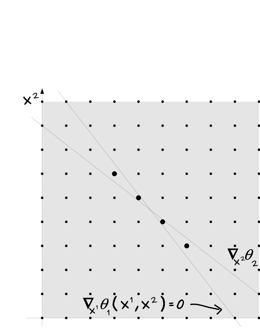
Figure 1: Equilibria for Example 2.1.

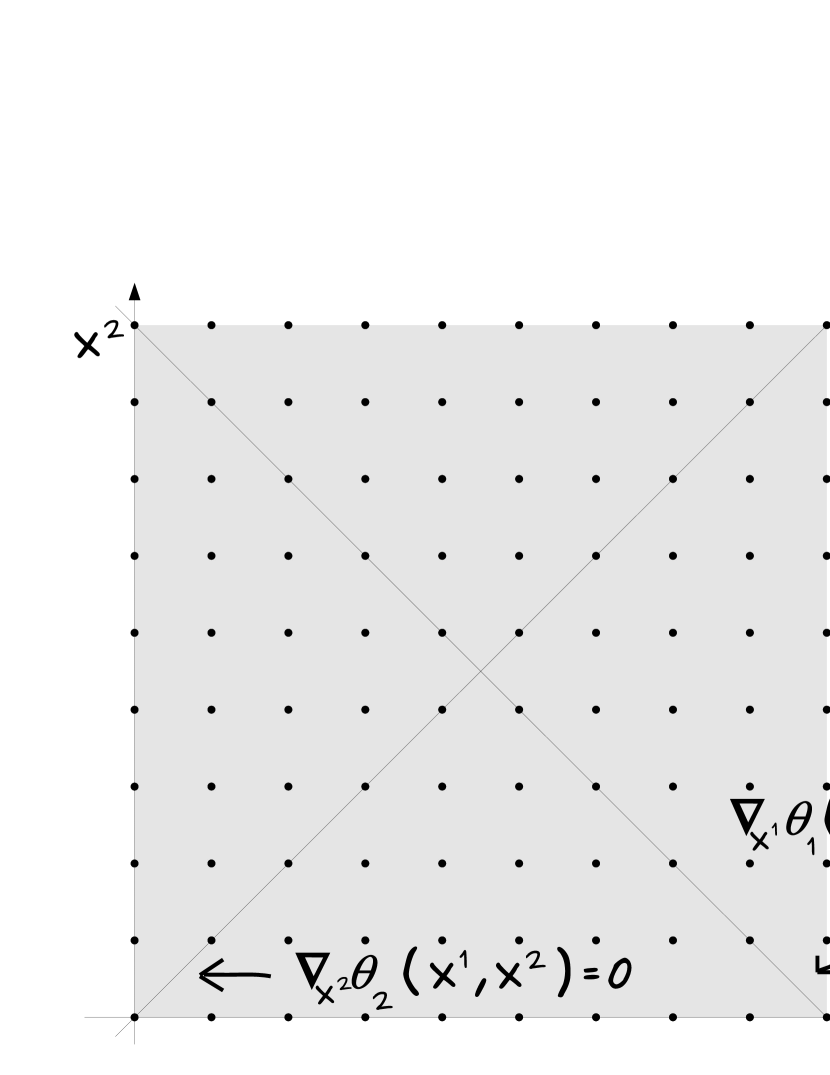
Figure 2: Lack of equilibria in Example 2.3.

Being $JF(x^{1},x^{2})=\left(\begin{array}[]{cc}9&7\\ 7&9\end{array}\right)$ symmetric, function $f(x^{1},x^{2})=\frac{9}{2}(x^{1})^{2}+7x^{1}x^{2}+\frac{9}{2}(x^{2})^{2}-72x^{1}-72x^{2}$ is such that $\nabla_{(x^{1},x^{2})}f(x^{1},x^{2})=F(x^{1},x^{2})$ for all ${\bf x}\in X$. However, the optimization problem defined by

$$\begin{array}[]{c}\displaystyle\min_{(x^{1},x^{2})}\,f(x^{1},x^{2})=\frac{9}{2}(x^{1})^{2}+7x^{1}x^{2}+\frac{9}{2}(x^{2})^{2}-72x^{1}-72x^{2}\\ \text{ }\quad 0\leq x^{1}\leq 9\\ \text{ }\quad 0\leq x^{2}\leq 9\\ \text{ }\quad\quad(x^{1},x^{2})\in{\mathbb{Z}}^{2},\end{array}$$

has the following solutions: $(4,5)$ and $(5,4)$, but not $(3,6)$ and $(6,3)$.

In any case, it is straightforward to prove the contrary, i.e. that all solutions of discrete optimization problem (3) are equilibria for the discrete NEP defined by (1). And, therefore, we can say that a necessary, but not sufficient, condition for a point $\bar{\bf x}$ to be a solution of problem (3) is to be a solution of the discrete NEP defined by (1).

Reformulating a dicrete NEP by using KKT conditions or variational inequalities is not fruitful, since first order optimality conditions cannot be effectively used with discrete strategy sets. However it is easy to see that relaxing integrality and then solving the resulting continuous NEP, defined by (2), may produce an integer solution, which then is also a solution for the original discrete game defined by (1). The following proposition, whose proof is trivial and therefore omitted, formalizes this issue.

Proposition 2.2.

Let ${\bf y}_{*}\in X\cap{\mathbb{Z}}^{n}$ be such that for all $\nu\in\{1,\ldots,N\}$:

$$\theta_{\nu}(y^{\nu}_{*},{\bf y}^{-\nu}_{*})\leq\theta_{\nu}(x^{\nu},{\bf y}^{-\nu}_{*}),\qquad\forall\,x^{\nu}\in X^{\nu},$$

that is ${\bf y}_{*}$ is a solution of the continuous NEP. Then it holds that for all $\nu\in\{1,\ldots,N\}$:

$$\theta_{\nu}(y^{\nu}_{*},{\bf y}^{-\nu}_{*})\leq\theta_{\nu}(x^{\nu},{\bf y}^{-\nu}_{*}),\qquad\forall\,x^{\nu}\in X^{\nu}\cap{\mathbb{Z}}^{n_{\nu}},$$

that is ${\bf y}_{*}$ is a solution of the discrete NEP. In particular, we say that ${\bf y}_{*}$ is a favorable solution for the discrete NEP.

In general, favorable solutions (defined in Proposition 2.2) are only a subset of the solution set of a discrete NEP. Moreover, very often, a discrete NEP can have more than one solution, but not favorable ones. In Example 2.1 this occurs, in that, none equilibrium of the discrete NEP is a favorable solution since, by relaxing the integrality contraints, the corresponding continuous NEP has the unique solution $(4.5,4.5)\notin{\mathbb{Z}}^{2}$, see Figure 2.

It is not easy to give conditions ensuring the existence of solutions for discrete NEPs in their general form. In fact, unlike for continuous problems, neither compactness of feasible set $X$, nor strong monotonicity of operator $F$, nor both together, can guarantee the existence of at least one solution, see Example 2.3.

Example 2.3.

There are two players each controlling one variable. Players’ problems are

$$\begin{array}[]{cccc}\displaystyle\min_{x^{1}}\,\theta_{1}(x^{1},x^{2})=\frac{1}{2}(x^{1})^{2}+x^{1}x^{2}-9x^{1}&&&\displaystyle\min_{x^{2}}\,\theta_{2}(x^{1},x^{2})=\frac{1}{2}(x^{2})^{2}-x^{1}x^{2}\\ \text{ }\quad 0\leq x^{1}\leq 9&&&\quad\text{ }\quad 0\leq x^{2}\leq 9\\ \text{ }\quad x^{1}\in{\mathbb{Z}}&&&\quad\text{ }\quad x^{2}\in{\mathbb{Z}}.\end{array}$$

Note that $0\leq x^{1}\leq 9$ and $0\leq x^{2}\leq 9$ define a compact set and that operator $F$ is strongly monotone. However the problem does not have any equilibrium, see Figure 2.

The most obvious way in order to give sufficient conditions for the existence of equilibria of a discrete NEP is to prove that at least one favorable solution exists. Following this reasoning, some researchers had considered discrete NEPs, then written down their KKT conditions, by previously relaxing integrality constraints, and finally given conditions ensuring that at least one of these KKT points is integer, see e.g. [18]. As said above, favorable solutions are only a subset (often empty) of the whole solution set of a discrete NEP, therefore it is worth to give conditions for the existence of solutions without assuming that these are favorable ones. We have to cite the works of Yang et al., [20, 29], that, by developing a theory on discrete nonlinear complementarity problems, proposed an alternative way to guarantee the existence of at least one equilibrium of discrete NEPs coming from some economic applications. However, results given in [29] are quite technical, and is rather difficult to use them in order to define general classes of problems for which existence can be proven. One important contribution on this topic was given by Topkis, [28], that, by studying supermodular games, defined a class of discrete NEPs that have at least one solution. In Section 4, we give conditions for the existence of equilibria (not only favorable ones) for a new class of discrete NEPs and we compare with results in [28] and in [29].

Notation: $M\in\mathbb{M}_{m\times n}$ is a matrix with $m$ rows and $n$ columns; $M_{j*}$ denotes the $j$-th row of $M$ and $M_{*i}$ denotes the $i$-th column of $M$; given a set of row indices $J_{r}$ and a set of column indices $J_{c}$, $M_{J_{r}J_{c}}$ is the submatrix with rows in $J_{r}$ and columns in $J_{c}$.

3 A branching method for finding all equilibria

In this section we present a method for finding all solutions of the discrete NEP defined by (1). This method mimics the branch and bound paradigm for discrete and combinatorial optimization problems. It consists of a systematic enumeration of candidate solutions by means of strategy space search: the set of candidate solutions is thought of as forming a rooted tree with the full set at the root. The algorithm explores branches of this tree, and during the enumeration of the candidate solutions a procedure is used in order to reduce the strategy set, in particular by fixing some variables.

It is important to say that bounding strategies, which are standard for discrete and combinatorial optimization problems, in general cannot be easily applied for discrete NEPs because of the difficulty to compute a lower bound for a suitable merit function. Standard merit fuctions for contiuous NEPs, see e.g. [14], not only cannot be directly applied in a discrete framework, but neither are easy to optimize. So, computing a lower bound for a merit function in a subset of the feasible discrete region needs, except in special cases, a complete enumeration. The situation is obviously much easier when $JF({\bf x})$ is symmetric for all ${\bf x}\in X$ since, as said before, a solution of the discrete NEP can be found by solving problem (3), and then $f({\bf x})$ can be an “easy” merit function. A similar situation also occurs in potential games, see [15]. However here we consider the general case and therefore given a subset of the strategy space it is very difficult to say if it cannot contain an equilibrium by using a standard bounding method.

The method we propose is defined below, but, before, we have to define some tools that it uses:

• an oracle ${\cal O}$ that takes a point $\bar{\bf x}\in X\cap{\mathbb{Z}}^{n}$ and outputs YES if and only if $\bar{\bf x}$ is an equilibrium for the discrete NEP defined by (1);

• a procedure ${\cal S}$ that, given a convex set $Y$ such that

  $$Y^{\nu}\subseteq X^{\nu},\qquad Y:=\prod_{\nu=1}^{N}Y^{\nu},$$ (4)

  yields one equilibrium of the continuous NEP in which each player $\nu$ solves

  $$\begin{array}[]{l}\min_{x^{\nu}}\theta_{\nu}(x^{\nu},{\bf x}^{-\nu})\\[5.0pt] \quad x^{\nu}\in Y^{\nu};\end{array}$$ (5)

• a procedure ${\cal F}$ that, given set $Y$ defined in (4) and a point $\bar{\bf x}$ returned by procedure ${\cal S}$, yields a closed, possibly unbounded, box $B$ such that set $Y\setminus B$ does not contain any equilibrium of the discrete NEP defined by (1);

• a procedure ${\cal C}$ that, given set $Y$ defined in (4) and a point $\bar{\bf x}\in Y\cap{\mathbb{Z}}^{n}$, yields $p$ closed, maybe unbounded, boxes $\bar{B}_{i}$ such that $\bar{\bf x}\notin\cup_{i=1}^{p}\bar{B}_{i}$, that $\bar{B}_{i}\cap\bar{B}_{j}=\emptyset$ for all $i\neq j$, and that $\tilde{\bf x}\in\cup_{i=1}^{p}\bar{B}_{i}$ for all $\tilde{\bf x}\in Y\cap{\mathbb{Z}}^{n}$, $\tilde{\bf x}\neq\bar{\bf x}$.

Later in this section we will discuss more in detail about these tools, now we are ready to define the branching method for finding all solutions of the discrete NEP defined by (1).

Algorithm 3.1.

(Branching Method)

(S.0)

Initialize list of strategy subsets ${\cal L}:=\{X\}$ and set of equilibria $E:=\emptyset$.

(S.1)

Take from ${\cal L}$ a strategy set $Y$.

(S.2)

Use ${\cal S}$ to obtain a solution $\bar{\bf x}$ of the continuous NEP defined by (5).

(S.3)

Use ${\cal F}$, with $Y$ and $\bar{\bf x}$, to obtain box $B$.

(S.4)

If $\bar{\bf x}\in{\mathbb{Z}}^{n}$ then use ${\cal O}$ on $\bar{\bf x}$: if ${\cal O}$ says YES then put $\bar{\bf x}$ in $E$.

(S.5)

If $\bar{\bf x}\in{\mathbb{Z}}^{n}$ then use ${\cal C}$, with $Y$ and $\bar{\bf x}$, to obtain $p$ boxes $\bar{B}_{i}$;
for all $i\in\{1,\ldots,p\}$, if $Y\cap B\cap\bar{B}_{i}\neq\emptyset$ then put it in ${\cal L}$;
go to (S.7).

(S.6)

Find an index $i\in\{1,\ldots,n\}$ such that $\bar{\bf x}_{i}\notin{\mathbb{Z}}$;
if $Y\cap B\cap\{{\bf x}\in{\mathbb{R}}^{n}:{\bf x}_{i}\geq\lceil\bar{\bf x}_{i}\rceil\}\neq\emptyset$ then put it in ${\cal L}$;
if $Y\cap B\cap\{{\bf x}\in{\mathbb{R}}^{n}:{\bf x}_{i}\leq\lfloor\bar{\bf x}_{i}\rfloor\}\neq\emptyset$ then put it in ${\cal L}$.

(S.7)

If ${\cal L}=\emptyset$ then STOP, else go to (S.1).

Eventually Algorithm 3.1 enumerates all points in $X\cap{\mathbb{Z}}^{n}$, checking their optimality, except those that are cut off by using procedure ${\cal F}$. Therefore, it is clear that: (i) if $X$ is compact, Algorithm 3.1 computes the whole solution set of the discrete NEP and (ii) procedure ${\cal F}$ is crucial in order to obtain an efficient algorithm.

On the other hand, if we are interested in computing only one equilibrium of the discrete NEP, and not the whole solution set, then we can stop Algorithm 3.1 as soon as it finds a solution, so considerably increasing efficiency of the method.

Now we describe in detail the tools used by Algorithm 3.1.

3.1 Oracle $\cal O$

Given a point $\bar{\bf x}\in{\mathbb{Z}}^{n}$, let us define the following best response at $\bar{\bf x}$ for each player $\nu$:

$$\hat{x}^{\nu}(\bar{\bf x}^{-\nu}):=\arg\min_{x^{\nu}\in X^{\nu}\cap{\mathbb{Z}}^{n_{\nu}}}\theta_{\nu}(x^{\nu},\bar{\bf x}^{-\nu}).$$ (6)

Oracle $\cal O$ must certify optimality of a point $\bar{\bf x}\in{\mathbb{Z}}^{n}$. Therefore, for all $\nu$, it checks if $\bar{x}^{\nu}\in\hat{x}^{\nu}({\bar{\bf x}}^{-\nu})$, and, if it is true, then answers YES, otherwise answers NO. Note that, in practice, computing a point in $\hat{x}^{\nu}({\bar{\bf x}}^{-\nu})$ could be a demanding task, since, in general, it requires to use a Mixed Integer Non-Linear Programming tool, see e.g. [2, 3, 24, 26]. In Section 5 we give specific implementation details on this issue.

3.2 Procedure $\cal S$

There are a lot of methods for finding a solution of a continuous NEP, see e.g. [6, 7, 14]. It is well known that if operator $F$ is monotone, or something a bit weaker, in the strategy set then there is more than one algorithm which is globally convergent to a solution of the continuous NEP. In Section 5 we give specific implementation details also on this issue.

3.3 Procedure $\cal F$

As said above, procedure ${\cal F}$ is crucial in order to obtain an efficient algorithm. First of all, let us analyze a situation that may set a trap. Suppose that $\bar{\bf x}\in{\mathbb{Z}}^{n}$ is a solution of the continuous NEP defined by (5), being $\bar{\bf x}$ integer then it is a favorable solution for the discrete NEP with strategy set $Y\subseteq X$, see Proposition 2.2. Moreover suppose that oracle $\cal O$ says that $\bar{\bf x}$ is not a solution of the discrete NEP defined by (1), which has strategy set $X\supseteq Y$. Then one could think that this is enough to say that $Y$ cannot contain any equilibrium of the discrete NEP defined by (1). But this is not true in general. Example 3.2 shows this in a very simple setting even with $F$ strongly monotone.

Example 3.2.

There are two players each controlling one variable. Players’ problems are

$$\begin{array}[]{cccc}\displaystyle\min_{x^{1}}\,\theta_{1}(x^{1},x^{2})=\frac{7}{16}(x^{1})^{2}-x^{1}x^{2}+\frac{1}{2}x^{1}&&&\displaystyle\min_{x^{2}}\,\theta_{2}(x^{1},x^{2})=\frac{1}{2}(x^{2})^{2}-\frac{3}{4}x^{1}x^{2}\\ \text{ }\quad-1\leq x^{1}\leq 2&&&\quad\text{ }\quad-1\leq x^{2}\leq 2\\ \text{ }\quad x^{1}\in{\mathbb{Z}}&&&\quad\text{ }\quad x^{2}\in{\mathbb{Z}}.\end{array}$$

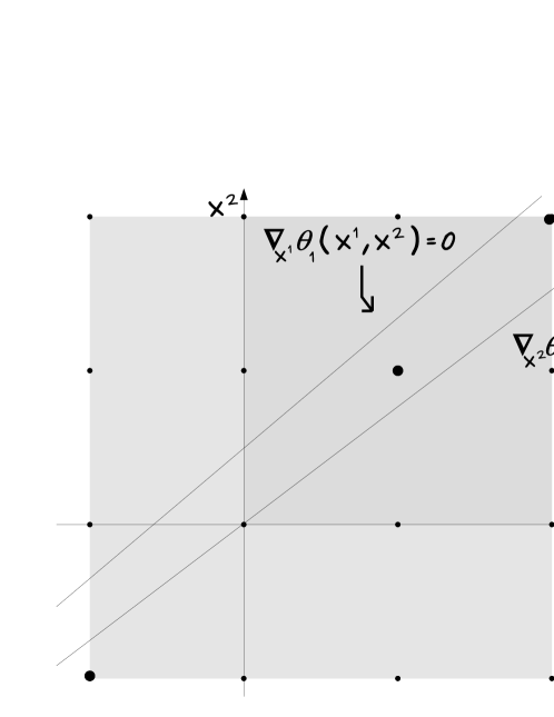
Figure 3: Equilibria for Example 3.2.

Then $X=\{x^{1},x^{2}\in{\mathbb{R}}:-1\leq x^{1}\leq 2,-1\leq x^{2}\leq 2\}$ and it holds that

$$JF(x^{1},x^{2})=\left(\begin{array}[]{cc}\;\;\,\frac{7}{8}&-1\\[5.0pt] -\frac{3}{4}&\;\;\,1\end{array}\right)\succ 0.$$

Let us indicate by $S\subseteq X\cap{\mathbb{Z}}^{n}$ the set of all solutions of this discrete NEP. Now let us consider $Y=\{x^{1},x^{2}\in{\mathbb{R}}:0\leq x^{1}\leq 2,0\leq x^{2}\leq 2\}\subset X$ and indicate by $\bar{S}\subseteq X$ the set of all solutions of the continuous NEP with strategy set $Y$ and with the same objective functions. Then it is easy to see that $S=\{(-1,-1),(1,1),(2,2)\}$ and $\bar{S}=\{(0,0)\}$, see Figure 3. Note that: $(0,0)\notin S$ and $S\supset\{(1,1),(2,2)\}\subset Y$.

Therefore procedure ${\cal F}$ cannot use this simple strategy in order to indentify a subset which provably does not contain any equilibrium. Procedure ${\cal F}$ we propose is motivated by the following proposition.

Proposition 3.3.

Suppose that $X$ is defined by box constraints:

$$X:=\left\{{\bf x}\in{\mathbb{R}}^{n}:{\bf l}\leq{\bf x}\leq{\bf u}\right\},\qquad{\bf l},{\bf u}\in{\mathbb{Z}}^{n}.$$ (7)

Let $\bar{\bf x}\in X\cap{\mathbb{Z}}^{n}$ be a solution for the continuous NEP defined by (2). Let us consider a generic player $\nu$. Suppose that an index $i\in\{1,\ldots,n_{\nu}\}$ exists such that one of the following two possibilities holds:

1. $F^{\nu}_{i}(\bullet)$ is a convex function, $\bar{x}^{\nu}_{i}=l^{\nu}_{i}$, and for each player $\mu\in\{1,\ldots,N\}$ and each index $j\in\{1,\ldots,n_{\mu}\}$, such that $(\mu,j)\neq(\nu,i)$:

   • if $\frac{\partial F^{\nu}_{i}(\bar{\bf x})}{\partial x^{\mu}_{j}}>0$ then $\bar{x}^{\mu}_{j}=l^{\mu}_{j}$,

   • if $\frac{\partial F^{\nu}_{i}(\bar{\bf x})}{\partial x^{\mu}_{j}}<0$ then $\bar{x}^{\mu}_{j}=u^{\mu}_{j}$.

2. $F^{\nu}_{i}(\bullet)$ is a concave function, $\bar{x}^{\nu}_{i}=u^{\nu}_{i}$ and for each player $\mu\in\{1,\ldots,N\}$ and each index $j\in\{1,\ldots,n_{\mu}\}$, such that $(\mu,j)\neq(\nu,i)$:

   • if $\frac{\partial F^{\nu}_{i}(\bar{\bf x})}{\partial x^{\mu}_{j}}>0$ then $\bar{x}^{\mu}_{j}=u^{\mu}_{j}$,

   • if $\frac{\partial F^{\nu}_{i}(\bar{\bf x})}{\partial x^{\mu}_{j}}<0$ then $\bar{x}^{\mu}_{j}=l^{\mu}_{j}$.

If $\theta_{\nu}$ is strictly convex with respect to $x^{\nu}_{i}$, then any point $\tilde{\bf x}\in X\cap{\mathbb{Z}}^{n}$ such that $\tilde{x}^{\nu}_{i}\neq\bar{x}^{\nu}_{i}$ cannot be an equilibrium for the discrete NEP defined by (1).

Proof.

Let $\bar{\tilde{{\bf x}}}\in X\cap{\mathbb{Z}}^{n}$ be such that $\bar{\tilde{x}}^{\nu}_{i}=\bar{x}^{\nu}_{i}$ and $\bar{\tilde{x}}^{\mu}_{j}=\tilde{x}^{\mu}_{j}$ for all $(\mu,j)\neq(\nu,i)$. And let $\tilde{\bar{{\bf x}}}\in X\cap{\mathbb{Z}}^{n}$ be such that $\tilde{\bar{x}}^{\nu}_{i}=\tilde{x}^{\nu}_{i}$ and $\tilde{\bar{x}}^{\mu}_{j}=\bar{x}^{\mu}_{j}$ for all $(\mu,j)\neq(\nu,i)$.

Let us assume that situation (i) holds: function $F^{\nu}_{i}(\bullet)$ is convex, then we can write

$$F^{\nu}_{i}(\bar{\tilde{{\bf x}}})-F^{\nu}_{i}(\bar{\bf x})\geq JF^{\nu}_{i}(\bar{\bf x})(\bar{\tilde{{\bf x}}}-\bar{\bf x}).$$

And then, by assumptions made in (i), it holds that

$$F^{\nu}_{i}(\bar{\bf x})\leq F^{\nu}_{i}(\bar{\tilde{{\bf x}}}).$$ (8)

The following chain of inequalities holds

$$0\overset{(A)}{\leq}F^{\nu}(\bar{\bf x})^{\scriptscriptstyle T}(\tilde{\bar{{\bf x}}}-\bar{\bf x})=F^{\nu}_{i}(\bar{\bf x})(\tilde{x}^{\nu}_{i}-\bar{x}^{\nu}_{i})\overset{(B)}{\leq}F^{\nu}_{i}(\bar{\tilde{{\bf x}}})(\tilde{x}^{\nu}_{i}-\bar{x}^{\nu}_{i})\overset{(C)}{<}\theta_{\nu}(\tilde{\bf x})-\theta_{\nu}(\bar{\tilde{{\bf x}}}),$$ (9)

where (A) holds since $\bar{\bf x}$ is a solution for the continuous NEP and $\tilde{\bar{{\bf x}}}$ is a feasible point; (B) follows from (8) and the fact that $\tilde{x}^{\nu}_{i}>\bar{x}^{\nu}_{i}$ since $\bar{x}^{\nu}_{i}=l^{\nu}_{i}$; (C) holds since $\theta_{\nu}$ is strictly convex with respect to $x^{\nu}_{i}$. Therefore $\theta_{\nu}(\tilde{\bf x})>\theta_{\nu}(\bar{\tilde{{\bf x}}})\in X\cap{\mathbb{Z}}^{n}$.

Now let us assume that situation (ii) holds: function $F^{\nu}_{i}(\bullet)$ is concave, then we can write

$$F^{\nu}_{i}(\bar{\tilde{{\bf x}}})-F^{\nu}_{i}(\bar{\bf x})\leq JF^{\nu}_{i}(\bar{\bf x})(\bar{\tilde{{\bf x}}}-\bar{\bf x}).$$

And then, by assumptions made in (ii), it holds that

$$F^{\nu}_{i}(\bar{\bf x})\geq F^{\nu}_{i}(\bar{\tilde{{\bf x}}}).$$ (10)

Then, by using (10) and with the same rationale of case (i), chain of inequalities (9) holds. Therefore we have the proof.

As said above procedure ${\cal F}$ is based on Proposition 3.3. Therefore it can be applied only when Algorithm 3.1 faces situations satisfying assumptions of Proposition 3.3. Let us assume, for simplicity, that

$$\theta_{\nu}({\bf x}):=\frac{1}{2}({x^{\nu}})^{\scriptscriptstyle T}Q^{\nu}x^{\nu}+\left(C^{\nu}{\bf x}^{-\nu}+b^{\nu}\right)^{\scriptscriptstyle T}x^{\nu},\quad\forall\,\nu\in\{1,\ldots,N\},$$ (11)

with $Q^{\nu}\in{\mathbb{M}}_{n_{\nu}\times n_{\nu}}$, $C^{\nu}\in{\mathbb{M}}_{n_{\nu}\times(n-n_{\nu})}$ and $b^{\nu}\in{\mathbb{R}}^{n_{\nu}}$ for all $\nu$. Moreover, let us assume that $X$ is defined as in (7). Then it is clear that, considering Algorithm 3.1, any strategy set $Y\in\cal L$ is a box. In this case, and by exploiting Proposition 3.3, procedure ${\cal F}$ can be defined as follows:

Algorithm 3.4.

(Procedure ${\cal F}$)

(Data)

A box strategy set $Y:=\{{\bf x}\in{\mathbb{R}}^{n}:{\bf l}\leq{\bf x}\leq{\bf u}\}$, with ${\bf l}\in{\mathbb{Z}}^{n}$ and ${\bf u}\in{\mathbb{Z}}^{n}$, and a solution $\bar{\bf x}$ of the continuous NEP defined by (5).

(S.0)

Set $B:={\mathbb{R}}^{n}$, $\nu:=1$ and $i:=1$.

(S.1)

If all the following conditions hold:

• $Q^{\nu}_{ii}>0$;

• $\bar{x}^{\nu}_{i}=l^{\nu}_{i}$;

• $\bar{x}^{\nu}_{j}=l^{\nu}_{j}$ for all $Q^{\nu}_{ij}>0$, $j=1,\ldots,n_{\nu}$, $j\neq i$;

• $\bar{x}^{\nu}_{j}=u^{\nu}_{j}$ for all $Q^{\nu}_{ij}<0$, $j=1,\ldots,n_{\nu}$, $j\neq i$;

• $\bar{\bf x}^{-\nu}_{j}={\bf l}^{-\nu}_{j}$ for all $C^{\nu}_{ij}>0$, $j=1,\ldots,(n-n_{\nu})$;

• $\bar{\bf x}^{-\nu}_{j}={\bf u}^{-\nu}_{j}$ for all $C^{\nu}_{ij}<0$, $j=1,\ldots,(n-n_{\nu})$;

then set $B:=B\cap\{{\bf x}\in{\mathbb{R}}^{n}:x^{\nu}_{i}\leq l^{\nu}_{i}\}$ and go to (S.3).

(S.2)

If all the following conditions hold:

• $Q^{\nu}_{ii}>0$;

• $\bar{x}^{\nu}_{i}=u^{\nu}_{i}$;

• $\bar{x}^{\nu}_{j}=u^{\nu}_{j}$ for all $Q^{\nu}_{ij}>0$, $j=1,\ldots,n_{\nu}$, $j\neq i$;

• $\bar{x}^{\nu}_{j}=l^{\nu}_{j}$ for all $Q^{\nu}_{ij}<0$, $j=1,\ldots,n_{\nu}$, $j\neq i$;

• $\bar{\bf x}^{-\nu}_{j}={\bf u}^{-\nu}_{j}$ for all $C^{\nu}_{ij}>0$, $j=1,\ldots,(n-n_{\nu})$;

• $\bar{\bf x}^{-\nu}_{j}={\bf l}^{-\nu}_{j}$ for all $C^{\nu}_{ij}<0$, $j=1,\ldots,(n-n_{\nu})$;

then set $B:=B\cap\{{\bf x}\in{\mathbb{R}}^{n}:x^{\nu}_{i}\geq u^{\nu}_{i}\}$.

(S.3)

Set $i:=i+1$; if $i\leq n_{\nu}$ then go to (S.1), else set $i:=1$.

(S.4)

Set $\nu:=\nu+1$; if $\nu\leq N$ then go to (S.1).

(Output)

Return $B$.

3.4 Procedure $\cal C$

This procedure is used in order to produce $p$ boxes $\bar{B}_{i}$ such that, given a point $\bar{\bf x}\in{\mathbb{Z}}^{n}$ and a strategy set $Y$, we obtain $\bar{\bf x}\notin\cup_{i=1}^{p}\bar{B}_{i}$, and $\bar{B}_{i}\cap\bar{B}_{j}=\emptyset$ for all $i\neq j$, and $\tilde{\bf x}\in\cup_{i=1}^{p}\bar{B}_{i}$ for all $\tilde{\bf x}\in Y\cap{\mathbb{Z}}^{n}$ with $\tilde{\bf x}\neq\bar{\bf x}$.

There are a lot of different implementations for this procedure. In this work we propose the following which yields $p=2n$ boxes.

Algorithm 3.5.

(Procedure ${\cal C}$)

(Data)

A point $\bar{\bf x}\in{\mathbb{Z}}^{n}$.

(S.0)

Set $\bar{B}_{i}:={\mathbb{R}}^{n}$, for all $i\in\{1,\ldots,2n\}$, and set $j:=1$.

(S.1)

Set:

• $\bar{B}_{2j-1}:=\bar{B}_{2j-1}\cap\{{\bf x}\in{\mathbb{R}}^{n}:\,{\bf x}_{j}\geq\bar{\bf x}_{j}+1\}$;

• $\bar{B}_{2j}:=\bar{B}_{2j}\cap\{{\bf x}\in{\mathbb{R}}^{n}:\,{\bf x}_{j}\leq\bar{\bf x}_{j}-1\}$;

• $\bar{B}_{t}:=\bar{B}_{t}\cap\{{\bf x}\in{\mathbb{R}}^{n}:\,{\bf x}_{j}=\bar{\bf x}_{j}\}$ for all $t\in{\mathbb{Z}}$ such that $2j+1\leq t\leq 2n$.

(S.2)

Set $j:=j+1$; if $j\leq n$ then go to (S.1).

(Output)

Return $\bar{B}_{i}$, $i=1,\ldots,2n$.

At this point, we have described all tools used by Algorithm 3.1, which, as said above, can be used to compute the whole solution set of any discrete NEP. Its efficiency is totally based on procedure $\cal F$ that prunes the branches of the search tree. In the next subsection, we propose an improved version of the branching algorithm, that, by using a preliminary procedure, shrinks the search area and drastically reduces the feasible points to be examined. However this improved algorithm can be used only if the problem has a particular structure.

3.5 An improved version of Algorithm 3.1

Here we propose an efficient algorithmic framework for finding all equilibria of discrete NEPs in which functions $\theta_{\nu}$ are defined as in (11) and $X$ is defined by box constraints as in (7). Note that many noncooperative games can be modeled as NEPs defined by (11) and (7), see e.g. [1]. This framework is composed of three parts: (i) compute lower bounds ${\bf l}^{*}\geq{\bf l}$ for the set of solutions, (ii) compute upper bounds ${\bf u}^{*}\leq{\bf u}$ for the set of solutions, and, then, (iii) use Algorithm 3.1 in order to get all solutions by exploring points in $[{\bf l}^{*},{\bf u}^{*}]\cap{\mathbb{Z}}^{n}$. The framework presented in this subsection is a great deal faster than just Algorithm 3.1 to compute either one equilibrium or the whole solution set of the discrete NEP. This is due to the effectiveness of the shrinkage of the search area: from $[{\bf l},{\bf u}]$ to $[{\bf l}^{*},{\bf u}^{*}]$.

The following Gauss-Seidel method performs the first task, that is computing lower bounds ${\bf l}^{*}$ for the set of solutions of the discrete NEP.

Algorithm 3.6.

(Gauss-Seidel Method to compute Solution Set Lower Bounds)

(S.0)

Set ${\bf w}:={\bf l}$ and ${\bf y}:={\bf l}$.

(S.1)

Set $\nu:=1$.

(S.2)

Set $i:=1$.

(S.3)

Set ${\bf z}\in{\mathbb{Z}}^{n}$ such that, for all $\mu\in\{1,\ldots,N\}$ and all $j\in\{1,\ldots,n_{\mu}\}$, $z^{\mu}_{j}:=y^{\mu}_{j}$ if $\frac{\partial F^{\nu}_{i}}{\partial x^{\mu}_{j}}\leq 0$ and $z^{\mu}_{j}:=u^{\mu}_{j}$ otherwise.

(S.4)

Compute $s\in{\mathbb{Z}}$ such that $y^{\nu}_{i}\leq s\leq u^{\nu}_{i}$,

if $s+1\leq u^{\nu}_{i}$ then

$$\theta_{\nu}\left(\left(\begin{array}[]{c}z^{\nu}_{1}\\ \vdots\\ z^{\nu}_{i-1}\\[10.00002pt] s\\[10.00002pt] z^{\nu}_{i+1}\\ \vdots\\ z^{\nu}_{n_{\nu}}\end{array}\right),{\bf z}^{-\nu}\right)\leq\theta_{\nu}\left(\left(\begin{array}[]{c}z^{\nu}_{1}\\ \vdots\\ z^{\nu}_{i-1}\\[10.00002pt] s+1\\[10.00002pt] z^{\nu}_{i+1}\\ \vdots\\ z^{\nu}_{n_{\nu}}\end{array}\right),{\bf z}^{-\nu}\right),$$ (12)

and if $y^{\nu}_{i}\leq s-1$ then

$$\theta_{\nu}\left(\left(\begin{array}[]{c}z^{\nu}_{1}\\ \vdots\\ z^{\nu}_{i-1}\\[10.00002pt] s-1\\[10.00002pt] z^{\nu}_{i+1}\\ \vdots\\ z^{\nu}_{n_{\nu}}\end{array}\right),{\bf z}^{-\nu}\right)>\theta_{\nu}\left(\left(\begin{array}[]{c}z^{\nu}_{1}\\ \vdots\\ z^{\nu}_{i-1}\\[10.00002pt] s\\[10.00002pt] z^{\nu}_{i+1}\\ \vdots\\ z^{\nu}_{n_{\nu}}\end{array}\right),{\bf z}^{-\nu}\right).$$ (13)

(S.5)

Set $y^{\nu}_{i}:=s$.

(S.6)

Set $i:=i+1$. If $i>n_{\nu}$ then set $\nu:=\nu+1$. If $\nu\leq N$ then go to (S.2).

(S.7)

If ${\bf w}={\bf y}$ then STOP and return ${\bf l}^{*}:={\bf y}$. Else set ${\bf w}:={\bf y}$ and go to (S.1).

The following theorem states that point ${\bf l}^{*}$ returned by Algorithm 3.6 is a lower bound for the set of solutions of the discrete NEP.

Theorem 3.7.

Suppose that $\theta_{\nu}$ are defined as in (11) and that $X$ is non-empty, bounded and defined as in (7).

Then Algorithm 3.6 returns point ${\bf l}^{*}$ in a finite number of iterations and for any solution ${\bf x}^{*}$ of the discrete NEP, defined by (1), it holds that ${\bf l}^{*}\leq{\bf x}^{*}$.

Proof.

At (S.5) of the first iteration of the algorithm, let us consider any point $\bar{\bf x}\in X\cap{\mathbb{Z}}^{n}$ such that $\bar{x}^{1}_{1}<y^{1}_{1}$ and the corresponding point $\tilde{\bf x}\in X\cap{\mathbb{Z}}^{n}$ such that $\tilde{x}^{\nu}_{i}=\bar{x}^{\nu}_{i}$ for all $(\nu,i)\neq(1,1)$ and $\tilde{x}^{1}_{1}=y^{1}_{1}$.

By assumptions, it holds that

$$\sum_{j=2}^{n_{1}}Q^{1}_{1j}\bar{x}^{1}_{j}\leq\sum_{j=2}^{n_{1}}Q^{1}_{1j}z^{1}_{j},\qquad\text{ and, }\qquad C^{1}_{1*}\bar{\bf x}^{-1}\leq C^{1}_{1*}{\bf z}^{-1}.$$ (14)

The following chain of inequalities holds

$$\frac{1}{2}Q^{1}_{1\,1}\left(\bar{x}^{1}_{1}\right)^{2}-\frac{1}{2}Q^{1}_{1\,1}\left(y^{1}_{1}\right)^{2}\overset{(A)}{>}$$

$$\left(\displaystyle\sum_{j=2}^{n_{1}}Q^{1}_{1j}z^{1}_{j}+C^{1}_{1*}{\bf z}^{-1}+b^{1}\right)(y^{1}_{1}-\bar{x}^{1}_{1})\overset{(B)}{\geq}$$

$$\left(\displaystyle\sum_{j=2}^{n_{1}}Q^{1}_{1j}\bar{x}^{1}_{j}+C^{1}_{1*}\bar{\bf x}^{-1}+b^{1}\right)(y^{1}_{1}-\bar{x}^{1}_{1}),$$

where (A) holds by (13) and the convexity of $\theta_{1}$ with respect to $x^{1}_{1}$; (B) follows from (14) and $\bar{x}^{1}_{1}<y^{1}_{1}$. Therefore $\theta_{1}(\bar{\bf x})>\theta_{1}(\tilde{\bf x})$, and then $\bar{\bf x}$ cannot be an equilibrium of the discrete NEP.

By iterating this reasoning, by using the new lower bounds as soon as they are computed, and by noting that ${\bf y}\geq{\bf w}$ for all iterations, we get the proof.

The algorithm to compute upper bounds ${\bf u}^{*}$ for the set of solutions of the discrete NEP is specular. We report it for completeness.

Algorithm 3.8.

(Gauss-Seidel Method to compute Solution Set Upper Bounds)

(S.0)

Set ${\bf w}:={\bf u}$ and ${\bf y}:={\bf u}$.

(S.1)

Set $\nu:=1$.

(S.2)

Set $i:=1$.

(S.3)

Set ${\bf z}\in{\mathbb{Z}}^{n}$ such that, for all $\mu\in\{1,\ldots,N\}$ and all $j\in\{1,\ldots,n_{\mu}\}$, $z^{\mu}_{j}:=y^{\mu}_{j}$ if $\frac{\partial F^{\nu}_{i}}{\partial x^{\mu}_{j}}\leq 0$ and $z^{\mu}_{j}:=l^{\mu}_{j}$ otherwise.

(S.4)

Compute $s\in{\mathbb{Z}}$ such that $l^{\nu}_{i}\leq s\leq y^{\nu}_{i}$,

if $l^{\nu}_{i}\leq s-1$ then

$$\theta_{\nu}\left(\left(\begin{array}[]{c}z^{\nu}_{1}\\ \vdots\\ z^{\nu}_{i-1}\\[10.00002pt] s-1\\[10.00002pt] z^{\nu}_{i+1}\\ \vdots\\ z^{\nu}_{n_{\nu}}\end{array}\right),{\bf z}^{-\nu}\right)\geq\theta_{\nu}\left(\left(\begin{array}[]{c}z^{\nu}_{1}\\ \vdots\\ z^{\nu}_{i-1}\\[10.00002pt] s\\[10.00002pt] z^{\nu}_{i+1}\\ \vdots\\ z^{\nu}_{n_{\nu}}\end{array}\right),{\bf z}^{-\nu}\right),$$ (15)

and if $s+1\leq y^{\nu}_{i}$ then

$$\theta_{\nu}\left(\left(\begin{array}[]{c}z^{\nu}_{1}\\ \vdots\\ z^{\nu}_{i-1}\\[10.00002pt] s\\[10.00002pt] z^{\nu}_{i+1}\\ \vdots\\ z^{\nu}_{n_{\nu}}\end{array}\right),{\bf z}^{-\nu}\right)<\theta_{\nu}\left(\left(\begin{array}[]{c}z^{\nu}_{1}\\ \vdots\\ z^{\nu}_{i-1}\\[10.00002pt] s+1\\[10.00002pt] z^{\nu}_{i+1}\\ \vdots\\ z^{\nu}_{n_{\nu}}\end{array}\right),{\bf z}^{-\nu}\right).$$ (16)

(S.5)

Set $y^{\nu}_{i}:=s$.

(S.6)

Set $i:=i+1$. If $i>n_{\nu}$ then set $\nu:=\nu+1$. If $\nu\leq N$ then go to (S.2).

(S.7)

If ${\bf w}={\bf y}$ then STOP and return ${\bf u}^{*}:={\bf y}$. Else set ${\bf w}:={\bf y}$ and go to (S.1).

Algorithm 3.8 works under the same assumptions of Algorithm 3.6 and then we skip a formal convergence result.

We are now ready to define the improved algorithm to compute the whole solution set of the discrete NEP.

Algorithm 3.9.

(Improved Branching Method)

(S.1)

Compute ${\bf l}^{*}$ by using Algorithm 3.6.

(S.2)

Compute ${\bf u}^{*}$ by using Algorithm 3.8.

(S.3)

Compute the whole solution set of the discrete NEP by using Algorithm 3.1 and initializing ${\cal L}:=\{[{\bf l}^{*},{\bf u}^{*}]\}$.

In Section 5 we show that Algorithm 3.9 works very well in practice and effectively computes the whole solution set of discrete NEPs.

4 Fast algorithms and existence results for a class of discrete NEPs

In this section we define a class of discrete NEPs for which we can give stronger results, namely, existence of equilibria and a fast Jacobi-type method for computing one of their equilibria.

Definition 4.1.

We say that a discrete NEP is 2-groups partitionable if it satisfies the following conditions:

1. $X$ is defined by box constraints as in (7);

2. $\theta_{\nu}$ is defined, for each player $\nu$, as

   $$\theta_{\nu}(x^{\nu},{\bf x}^{-\nu}):=\theta^{P}_{\nu}(x^{\nu})+\Theta^{O}_{\nu}({\bf x}^{-\nu})^{\scriptscriptstyle T}x^{\nu},$$ (17)

   where $\theta_{\nu}^{P}:{\mathbb{R}}^{n_{\nu}}\to{\mathbb{R}}$ is defined in the following way

   $$\theta_{\nu}^{P}(x^{\nu}):=\sum_{i=1}^{n_{\nu}}\vartheta_{\nu,i}^{P}(x^{\nu}_{i})+\frac{1}{2}({x^{\nu}})^{\scriptscriptstyle T}Q^{\nu}x^{\nu},$$ (18)

   $\vartheta_{\nu,i}^{P}:{\mathbb{R}}\to{\mathbb{R}}$, for all $i$, and $Q^{\nu}\in{\mathbb{M}}_{n_{\nu}\times n_{\nu}}$, and $\Theta^{O}_{\nu}:{\mathbb{R}}^{n_{-\nu}}\to{\mathbb{R}}^{n_{\nu}}$ is an operator made up of convex or concave functions;

3. a partition of the variables indices in two groups, $G_{1}$ and $G_{2}$, exists such that

   $$\frac{\partial F^{\nu}_{i}({\bf x})}{\partial x^{\mu}_{j}}\leq 0,\;\forall\,{\bf x}\in X,\;\forall\,(\nu,i)\neq(\mu,j)\,:$$

   $$\qquad\qquad\qquad\qquad\qquad(\nu,i)\in G_{1}\ni(\mu,j)\text{ or }(\nu,i)\in G_{2}\ni(\mu,j),$$ (19)

   $$\frac{\partial F^{\nu}_{i}({\bf x})}{\partial x^{\mu}_{j}}\geq 0,\;\forall\,{\bf x}\in X,\;\forall\,(\nu,i)\neq(\mu,j)\,:$$

   $$\qquad\qquad\qquad\qquad\qquad(\nu,i)\in G_{1}\not\ni(\mu,j)\text{ or }(\nu,i)\in G_{2}\not\ni(\mu,j).$$ (20)

The following is an example of a 2-groups partitionable discrete NEP.

Example 4.2.

There are two players. The first player solves the following problem

$$\displaystyle\min_{x^{1}}\,\theta_{1}(x^{1},x^{2}) =\frac{1}{2}(x^{1})^{\scriptscriptstyle T}\left(\begin{array}[]{cc}3&1\\ 1&3\end{array}\right)x^{1}+(x^{1})^{\scriptscriptstyle T}\left(\begin{array}[]{cc}4&-3\\ -1&1\end{array}\right)x^{2}+(7\quad 2)x^{1}$$

$$\qquad\qquad-5\leq x^{1}\leq 5$$

$$\qquad\qquad\qquad x^{1}\in{\mathbb{Z}}^{2},$$

while the second player solves the following problem

$$\displaystyle\min_{x^{2}}\,\theta_{2}(x^{1},x^{2}) =\frac{1}{2}(x^{2})^{\scriptscriptstyle T}\left(\begin{array}[]{cc}2&1\\ 1&2\end{array}\right)x^{2}+(x^{2})^{\scriptscriptstyle T}\left(\begin{array}[]{cc}1&-2\\ -3&4\end{array}\right)x^{1}+(5\quad 6)x^{2}$$

$$\qquad\qquad-5\leq x^{2}\leq 5$$

$$\qquad\qquad\qquad x^{2}\in{\mathbb{Z}}^{2}.$$

By partitioning variables in this way: $G_{1}=\{(1,1),(2,2)\}$, $G_{2}=\{(1,2),(2,1)\}$, then (19) and (20) are satisfied.

Note that also the problems in Examples 2.1 and 3.2 are 2-groups partitionable discrete NEPs.

In order to give an economic interpretation of condition (iii) in Definition 4.1, let us consider a standard pricing game. There are $N$ firms that compete in the same market in order to increase their profits as much as possible. Each firm $\nu$ produces a single product and sets its price $p^{\nu}\in{\mathbb{Z}}$. The prices are considered as integer, rather than real, variables in order to get the model more realistic, since the price of a product cannot be specified more closely than the minimum unit of a currency. For the sake of simplicity, let us assume that the consumers demand function for each firm $\nu$ is linear:

$$D_{\nu}(p^{\nu},{\bf p}^{-\nu}):=a_{\nu}-b_{\nu}p^{\nu}+(c^{\nu})^{\scriptscriptstyle T}{\bf p}^{-\nu},$$

where $a_{\nu},\,b_{\nu}\in{\mathbb{R}}_{+}$ and $c^{\nu}\in{\mathbb{R}}^{N-1}$. Moreover, assume that there are no fixed costs of production and marginal cost $d_{\nu}$ for each firm $\nu$ is such that $0<d_{\nu}<a_{\nu}$. Therefore, for each firm $\nu$, since the objective is to maximize its profit $D_{\nu}(p^{\nu},{\bf p}^{-\nu})(p^{\nu}-d_{\nu})$, the optimization problem to solve is the following:

$$\displaystyle\min_{p^{\nu}} \;b_{\nu}(p^{\nu})^{2}-({\bf p}^{-\nu})^{\scriptscriptstyle T}c^{\nu}p^{\nu}-(a_{\nu}+b_{\nu}d_{\nu})p^{\nu}$$

$$0\leq p^{\nu}\leq P_{\nu},\quad p^{\nu}\in{\mathbb{Z}},$$

where $P_{\nu}\in{\mathbb{Z}}$ is a suitable upper bound. Clearly this discrete NEP satisfies conditions (i) and (ii) in Definition 4.1. Condition (iii) in Definition 4.1 simply requires that two groups of products $G_{1}$ and $G_{2}$ exist such that: two products of firms $\nu$ and $\mu$ belonging to the same group are substitutes (that is $c^{\nu}_{\mu}\geq 0$ and $c^{\mu}_{\nu}\geq 0$), while two products of firms $\nu$ and $\mu$ belonging to different groups are complements (that is $c^{\nu}_{\mu}\leq 0$ and $c^{\mu}_{\nu}\leq 0$).

Let us consider the following Jacobi-type method:

Algorithm 4.3.

(Jacobi-type Method)

(S.0)

Choose a starting point ${\bf x}^{0}\in X\cap{\mathbb{Z}}^{n}$ and set $k:=0$.

(S.1)

If ${\bf x}^{k}$ is a solution of the discrete NEP then STOP.

(S.2)

Choose a subset ${\cal J}^{k}$ of the players. For each $\nu\in{\cal J}^{k}$ compute a best response ${\hat{x}}^{k,\nu}$:

$${\hat{x}}^{k,\nu}\in\hat{x}^{\nu}({\bf x}^{k,-\nu}).$$

(S.3)

For all $\nu\in{\cal J}^{k}$ set $x^{k+1,\nu}:=\hat{x}^{k,\nu}$ and for all $\nu\notin{\cal J}^{k}$ set $x^{k+1,\nu}:=x^{k,\nu}$.
Set $k:=k+1$ and go to (S.1).

We recall that $\hat{x}^{\nu}(\bullet)$ is defined in (6). This type of methods are very popular among practitioners of Nash problems and their rationale is particularly simple to grasp since they are the most “natural” decomposition methods. Algorithm 4.3 can be easily implemented in a parallel framework in order to reduce the computational burden at (S.2). Furthermore, it has a non-standard feature that gives an additional degree of freedom compared to traditional Jacobi-type schemes: the choice of subset ${\cal J}^{k}$ of the players that “play” at iteration $k$. We can say that it is an incomplete Jacobi-type iteration. As special cases, by selecting only one player at each iteration we get a Gauss-Southwell scheme, while by selecting roundly each single player we get a Gauss-Seidel scheme.

Theorem 4.4.

Suppose that (19) and (20) hold and that, for each player $\nu$, $\theta_{\nu}$ is defined as in (17), where $\theta_{\nu}^{P}$ is defined as in (18) and $\Theta^{O}_{\nu}$ is an operator made up of convex or concave functions. Suppose that $X$ is non-empty, bounded and defined by box constraints as in (7).

For all $\nu\in\{1,\ldots,N\}$ and all $i\in\{1,\ldots,n_{\nu}\}$, let $x^{0,\nu}_{i}:=l^{\nu}_{i}$ if $(\nu,i)\in G_{1}$ and let $x^{0,\nu}_{i}:=u^{\nu}_{i}$ if $(\nu,i)\in G_{2}$. Let a finite positive integer $h$ exists such that $\nu\in\cup_{t=k}^{k+h}{\cal J}^{t}$ for each player $\nu$ and each iterate $k$.

Then, for each iterate $k$ and each player $\nu\in{\cal J}^{k}$, a best response $\hat{x}^{k,\nu}\in\hat{x}^{\nu}({\bf x}^{k,-\nu})$ can be computed such that

$$\hat{x}^{k,\nu}_{i}\geq x^{k,\nu}_{i},\quad\forall\,(\nu,i)\in G_{1},\qquad\hat{x}^{k,\nu}_{i}\leq x^{k,\nu}_{i},\quad\forall\,(\nu,i)\in G_{2}.$$ (21)

By computing $\hat{x}^{k,\nu}$ for all $k$ and all $\nu\in{\cal J}^{k}$ such that (21) holds, Algorithm 4.3 converges in a finite number of iterations to a solution of the discrete NEP defined by (1).

Proof.

First of all note that, by assumptions on $X$, set $\hat{x}^{\nu}(\bar{\bf x}^{-\nu})$ is non-empty and finite for any $\nu$ and any $\bar{\bf x}^{-\nu}$. However, it is easy to see that $\hat{x}^{\nu}(\bar{\bf x}^{-\nu})$ may contain more than one element.

Let us consider the first iteration. Since ${\bf x}^{1}\in X\cap{\mathbb{Z}}^{n}$ then it holds that $x^{1,\nu}_{i}\geq x^{0,\nu}_{i}$ if $(\nu,i)\in G_{1}$, and $x^{1,\nu}_{i}\leq x^{0,\nu}_{i}$ if, otherwise, $(\nu,i)\in G_{2}$. For all $\nu$ and all $i\in\{1,\ldots,n_{\nu}\}$ such that $(\nu,i)\in G_{1}$, if $\Theta_{\nu,i}^{O}$ is a convex function, then we can write

$$\Theta_{\nu,i}^{O}({\bf x}^{0,-\nu})-\Theta_{\nu,i}^{O}({\bf x}^{1,-\nu})\geq\nabla\Theta_{\nu,i}^{O}({\bf x}^{1,-\nu})^{\scriptscriptstyle T}({\bf x}^{0,-\nu}-{{\bf x}^{1,-\nu}}),$$ (22)

otherwise, $\Theta_{\nu,i}^{O}$ is concave, and then we can write

$$\Theta_{\nu,i}^{O}({\bf x}^{1,-\nu})-\Theta_{\nu,i}^{O}({\bf x}^{0,-\nu})\leq\nabla\Theta_{\nu,i}^{O}({\bf x}^{0,-\nu})^{\scriptscriptstyle T}({\bf x}^{1,-\nu}-{{\bf x}^{0,-\nu}}).$$ (23)

In both cases, since, by (19), for all $\mu\neq\nu$ such that $(\mu,j)\in G_{1}$ it holds that

$$x^{1,\mu}_{j}\geq x^{0,\mu}_{j},\qquad\frac{\partial\Theta_{\nu,i}^{O}({\bf x}^{0,-\nu})}{\partial x^{\mu}_{j}}\leq 0,\qquad\frac{\partial\Theta_{\nu,i}^{O}({\bf x}^{1,-\nu})}{\partial x^{\mu}_{j}}\leq 0,$$

while, by (20), for all $\mu\neq\nu$ such that $(\mu,j)\in G_{2}$ it holds that

$$x^{1,\mu}_{j}\leq x^{0,\mu}_{j},\qquad\frac{\partial\Theta_{\nu,i}^{O}({\bf x}^{0,-\nu})}{\partial x^{\mu}_{j}}\geq 0,\qquad\frac{\partial\Theta_{\nu,i}^{O}({\bf x}^{1,-\nu})}{\partial x^{\mu}_{j}}\geq 0,$$

then, by (22) or (23), it holds that

$$\Theta_{\nu,i}^{O}({\bf x}^{1,-\nu})\leq\Theta_{\nu,i}^{O}({\bf x}^{0,-\nu}),\qquad\forall\,(\nu,i)\in G_{1}.$$ (24)

On the other hand, for all $\nu$ and all $i\in\{1,\ldots,n_{\nu}\}$ such that $(\nu,i)\in G_{2}$, if $\Theta_{\nu,i}^{O}$ is a convex function, then we can write

$$\Theta_{\nu,i}^{O}({\bf x}^{1,-\nu})-\Theta_{\nu,i}^{O}({\bf x}^{0,-\nu})\geq\nabla\Theta_{\nu,i}^{O}({\bf x}^{0,-\nu})^{\scriptscriptstyle T}({\bf x}^{1,-\nu}-{{\bf x}^{0,-\nu}}),$$ (25)

otherwise, $\Theta_{\nu,i}^{O}$ is concave, and we can write

$$\Theta_{\nu,i}^{O}({\bf x}^{0,-\nu})-\Theta_{\nu,i}^{O}({\bf x}^{1,-\nu})\leq\nabla\Theta_{\nu,i}^{O}({\bf x}^{1,-\nu})^{\scriptscriptstyle T}({\bf x}^{0,-\nu}-{{\bf x}^{1,-\nu}}).$$ (26)

Then, by (20), for all $\mu\neq\nu$ such that $(\mu,j)\in G_{1}$ it holds that

$$x^{1,\mu}_{j}\geq x^{0,\mu}_{j},\qquad\frac{\partial\Theta_{\nu,i}^{O}({\bf x}^{0,-\nu})}{\partial x^{\mu}_{j}}\geq 0,\qquad\frac{\partial\Theta_{\nu,i}^{O}({\bf x}^{1,-\nu})}{\partial x^{\mu}_{j}}\geq 0,$$

while, by (19), for all $\mu\neq\nu$ such that $(\mu,j)\in G_{2}$ it holds that

$$x^{1,\mu}_{j}\leq x^{0,\mu}_{j},\qquad\frac{\partial\Theta_{\nu,i}^{O}({\bf x}^{0,-\nu})}{\partial x^{\mu}_{j}}\leq 0,\qquad\frac{\partial\Theta_{\nu,i}^{O}({\bf x}^{1,-\nu})}{\partial x^{\mu}_{j}}\leq 0,$$

then, by (25) or (26), it holds that

$$\Theta_{\nu,i}^{O}({\bf x}^{1,-\nu})\geq\Theta_{\nu,i}^{O}({\bf x}^{0,-\nu}),\qquad\forall\,(\nu,i)\in G_{2}.$$ (27)

Now let us consider the second iteration. In order to prove that, for all $\nu$, a best response $\hat{x}^{1,\nu}\in\hat{x}^{\nu}({\bf x}^{1,-\nu})$ exists such that for all $i\in\{1,\ldots,n_{\nu}\}$:

$$\hat{x}^{1,\nu}_{i}\geq x^{1,\nu}_{i},\quad\text{ if }\,(\nu,i)\in G_{1},\qquad\text{ and, }\qquad\hat{x}^{1,\nu}_{i}\leq x^{1,\nu}_{i},\quad\text{ if }\,(\nu,i)\in G_{2},$$ (28)

we have to consider two possibilities. If $\nu\notin{\cal J}^{0}$ then $x^{1,\nu}=x^{0,\nu}$ and then (28) is trivially satisfied. Otherwise $\nu\in{\cal J}^{0}$ and we suppose by contradiction that for all $y^{\nu}\in\hat{x}^{\nu}({\bf x}^{1,-\nu})$ a non-empty set of indices $J\subseteq\{1,\ldots,n_{\nu}\}$ exists such that for all $i\in J$ it holds that $y^{\nu}_{i}<x^{1,\nu}_{i}$ if $(\nu,i)\in G_{1}$ and $y^{\nu}_{i}>x^{1,\nu}_{i}$ if $(\nu,i)\in G_{2}$. Now we show that this is impossible. Let $\bar{J}:=\{1,\ldots,n_{\nu}\}\setminus J$, for all $j\in\bar{J}$ we have $y^{\nu}_{j}\geq x^{1,\nu}_{j}$ if $(\nu,j)\in G_{1}$ and $y^{\nu}_{j}\leq x^{1,\nu}_{j}$ if $(\nu,j)\in G_{2}$. We define $\bar{y}^{\nu},\tilde{y}^{\nu}\in{\mathbb{Z}}^{n_{\nu}}$ such that $\bar{y}^{\nu}_{J}=y^{\nu}_{J}$, $\bar{y}^{\nu}_{\bar{J}}=x^{1,\nu}_{\bar{J}}$, $\tilde{y}^{\nu}_{J}=x^{1,\nu}_{J}$ and $\tilde{y}^{\nu}_{\bar{J}}=y^{\nu}_{\bar{J}}$. It is easy to see that both $\bar{y}^{\nu}$ and $\tilde{y}^{\nu}$ are feasible for player $\nu$, since $X$ is a box. In order to show that

$$\left(\theta_{\nu}^{P}(\tilde{y}^{\nu})-\theta_{\nu}^{P}(y^{\nu})\right)-\left(\theta_{\nu}^{P}(x^{1,\nu})-\theta_{\nu}^{P}(\bar{y}^{\nu})\right)\leq 0,$$ (29)

we consider the following two chains of inequalities:

$$\left[\frac{1}{2}({\tilde{y}^{\nu}})^{\scriptscriptstyle T}Q^{\nu}\tilde{y}^{\nu}-\frac{1}{2}({y^{\nu}})^{\scriptscriptstyle T}Q^{\nu}y^{\nu}\right]-\left[\frac{1}{2}(x^{1,\nu})^{\scriptscriptstyle T}Q^{\nu}(x^{1,\nu})-\frac{1}{2}({\bar{y}^{\nu}})^{\scriptscriptstyle T}Q^{\nu}\bar{y}^{\nu}\right]=$$

$$\left[\left((y^{\nu}_{J})^{\scriptscriptstyle T}\;(y^{\nu}_{\bar{J}})^{\scriptscriptstyle T}\right)\,\left(\begin{array}[]{c}Q^{\nu}_{JJ}\\ Q^{\nu}_{\bar{J}J}\end{array}\right)\,\left(x^{1,\nu}_{J}-y^{\nu}_{J}\right)+\frac{1}{2}\left(x^{1,\nu}_{J}-y^{\nu}_{J}\right)^{\scriptscriptstyle T}Q^{\nu}_{JJ}\left(x^{1,\nu}_{J}-y^{\nu}_{J}\right)\right]-$$

$$\left[\left((y^{\nu}_{J})^{\scriptscriptstyle T}\;(x^{1,\nu}_{\bar{J}})^{\scriptscriptstyle T}\right)\,\left(\begin{array}[]{c}Q^{\nu}_{JJ}\\ Q^{\nu}_{\bar{J}J}\end{array}\right)\,\left(x^{1,\nu}_{J}-y^{\nu}_{J}\right)+\frac{1}{2}\left(x^{1,\nu}_{J}-y^{\nu}_{J}\right)^{\scriptscriptstyle T}Q^{\nu}_{JJ}\left(x^{1,\nu}_{J}-y^{\nu}_{J}\right)\right]=$$

$$\left(y^{\nu}_{\bar{J}}-x^{1,\nu}_{\bar{J}}\right)^{\scriptscriptstyle T}Q^{\nu}_{\bar{J}J}\left(x^{1,\nu}_{J}-y^{\nu}_{J}\right)\leq 0,$$

where the last inequality holds because:

• for all $j\in\bar{J}$: $\left(y^{\nu}_{j}-x^{1,\nu}_{j}\right)\geq 0$ if $(\nu,j)\in G_{1}$ and $\left(y^{\nu}_{j}-x^{1,\nu}_{j}\right)\leq 0$ if $(\nu,j)\in G_{2}$,

• for all $j\in\bar{J}$ and all $i\in J$: $Q^{\nu}_{ji}\leq 0$ if $(\nu,j)\in G_{1}\ni(\nu,i)$ or $(\nu,j)\in G_{2}\ni(\nu,i)$, by (19), and $Q^{\nu}_{ji}\geq 0$ if $(\nu,j)\in G_{1}\not\ni(\nu,i)$ or $(\nu,j)\in G_{2}\not\ni(\nu,i)$, by (20),

• for all $i\in J$: $\left(x^{1,\nu}_{i}-y^{\nu}_{i}\right)>0$ if $(\nu,i)\in G_{1}$ and $\left(x^{1,\nu}_{i}-y^{\nu}_{i}\right)<0$ if $(\nu,i)\in G_{2}$;

the other chain is the following:

$$\sum_{i=1}^{n_{\nu}}\vartheta_{\nu,i}^{P}(\tilde{y}^{\nu}_{i})-\sum_{i=1}^{n_{\nu}}\vartheta_{\nu,i}^{P}(y^{\nu}_{i})-\sum_{i=1}^{n_{\nu}}\vartheta_{\nu,i}^{P}(x^{1,\nu}_{i})+\sum_{i=1}^{n_{\nu}}\vartheta_{\nu,i}^{P}(\bar{y}^{\nu}_{i})=$$

$$\left(\sum_{i\in J}\vartheta_{\nu,i}^{P}(x^{1,\nu}_{i})+\sum_{i\in\bar{J}}\vartheta_{\nu,i}^{P}(y^{\nu}_{i})\right)-\sum_{i=1}^{n_{\nu}}\vartheta_{\nu,i}^{P}(y^{\nu}_{i})-\sum_{i=1}^{n_{\nu}}\vartheta_{\nu,i}^{P}(x^{1,\nu}_{i})+$$

$$\quad\left(\sum_{i\in J}\vartheta_{\nu,i}^{P}(y^{\nu}_{i})+\sum_{i\in\bar{J}}\vartheta_{\nu,i}^{P}(x^{1,\nu}_{i})\right)=0;$$

therefore (29) holds. By using (29), we can write the following chain of inequalities

$$0 \geq\theta_{\nu}^{P}(\tilde{y}^{\nu})-\theta_{\nu}^{P}(y^{\nu})-\theta_{\nu}^{P}(x^{1,\nu})+\theta_{\nu}^{P}(\bar{y}^{\nu})$$

$$\overset{(A)}{\geq}\theta_{\nu}^{P}(\tilde{y}^{\nu})-\theta_{\nu}^{P}(y^{\nu})+\Theta_{\nu,J}^{O}({\bf x}^{0,-\nu})^{\scriptscriptstyle T}(x^{1,\nu}_{J}-y^{\nu}_{J})$$

$$\overset{(B)}{\geq}\theta_{\nu}^{P}(\tilde{y}^{\nu})-\theta_{\nu}^{P}(y^{\nu})+\Theta_{\nu,J}^{O}({\bf x}^{1,-\nu})^{\scriptscriptstyle T}(x^{1,\nu}_{J}-y^{\nu}_{J})$$

$$=\theta_{\nu}^{P}(\tilde{y}^{\nu})-\theta_{\nu}^{P}(y^{\nu})+\Theta_{\nu}^{O}({\bf x}^{1,-\nu})^{\scriptscriptstyle T}(\tilde{y}^{\nu}-y^{\nu}),$$

where (A) holds since $x^{1,\nu}\in\hat{x}^{\nu}({\bf x}^{0,-\nu})$ (remember that we are considering the case in which $\nu\in{\cal J}^{0}$) and $\bar{y}^{\nu}$ is feasible for player $\nu$; while (B) is true since for all $i\in J$: if $(\nu,i)\in G_{1}$ we have (24) and $(x^{1,\nu}_{i}-y^{\nu}_{i})>0$, and if $(\nu,i)\in G_{2}$ we have (27) and $(x^{1,\nu}_{i}-y^{\nu}_{i})<0$. Then we can conclude that $\theta_{\nu}(\tilde{y}^{\nu},{\bf x}^{1,-\nu})\leq\theta_{\nu}(y^{\nu},{\bf x}^{1,-\nu})$ and, since $\tilde{y}^{\nu}_{i}\geq x^{1,\nu}_{i}$ for all $(\nu,i)\in G_{1}$ and $\tilde{y}^{\nu}_{i}\leq x^{1,\nu}_{i}$ for all $(\nu,i)\in G_{2}$, this is a contradiction. Therefore, for all $\nu\in{\cal J}^{1}$, we can set $\hat{x}^{1,\nu}\in\hat{x}^{\nu}({\bf x}^{1,-\nu})$ satisfying (28) for all $i\in\{1,\ldots,n_{\nu}\}$, and then we obtain

$$x^{2,\nu}_{i}\geq x^{1,\nu}_{i},\quad\forall\,(\nu,i)\in G_{1},\qquad x^{2,\nu}_{i}\leq x^{1,\nu}_{i},\quad\forall\,(\nu,i)\in G_{2}.$$

At a generic iterate $k\geq 2$, assuming that for all $t<k$

$$x^{k,\nu}_{i}\geq x^{t,\nu}_{i},\quad\forall\,(\nu,i)\in G_{1},\qquad x^{k,\nu}_{i}\leq x^{t,\nu}_{i},\quad\forall\,(\nu,i)\in G_{2},$$

we can do similar considerations in order to prove that we can get for all $(\nu,i)$:

$$x^{k+1,\nu}_{i}\geq x^{k,\nu}_{i},\quad\text{ if }\,(\nu,i)\in G_{1},\qquad\text{ and, }\qquad x^{k+1,\nu}_{i}\leq x^{k,\nu}_{i},\quad\text{ if }\,(\nu,i)\in G_{2}.$$ (30)

In fact, we have the following two possibilities for any $\nu\in{\cal J}^{k}$: if $\nu\notin\cup_{t=0}^{k-1}{\cal J}^{t}$ then $x^{k,\nu}=x^{0,\nu}$ and then (30) is trivially satisfied, otherwise, as above we can contradict the fact that any point $y^{\nu}$ in $\hat{x}^{\nu}({\bf x}^{k,-\nu})$ has a non-empty set of indices $J$ such that for all $i\in J$ it holds that $y^{\nu}_{i}<x^{k,\nu}_{i}$ if $(\nu,i)\in G_{1}$ and $y^{\nu}_{i}>x^{k,\nu}_{i}$ if $(\nu,i)\in G_{2}$. We define $\bar{y}^{\nu}$ and $\tilde{y}^{\nu}$ as above. Let $p<k$ be the last iterate such that $\nu\in{\cal J}^{p}$. By the same considerations made above, we can write $\Theta_{\nu,i}^{O}({\bf x}^{k,-\nu})\leq\Theta_{\nu,i}^{O}({\bf x}^{p,-\nu})$ for all $(\nu,i)\in G_{1}$, $\Theta_{\nu,i}^{O}({\bf x}^{k,-\nu})\geq\Theta_{\nu,i}^{O}({\bf x}^{p,-\nu})$ for all $(\nu,i)\in G_{2}$, and $\left(\theta_{\nu}^{P}(\tilde{y}^{\nu})-\theta_{\nu}^{P}(y^{\nu})\right)-\left(\theta_{\nu}^{P}(x^{k,\nu})-\theta_{\nu}^{P}(\bar{y}^{\nu})\right)\leq 0$ and therefore, since $x^{k,\nu}=x^{p+1,\nu}$, the chain of inequalities

$$0 \geq\theta_{\nu}^{P}(\tilde{y}^{\nu})-\theta_{\nu}^{P}(y^{\nu})-\theta_{\nu}^{P}(x^{k,\nu})+\theta_{\nu}^{P}(\bar{y}^{\nu})$$

$$\geq\theta_{\nu}^{P}(\tilde{y}^{\nu})-\theta_{\nu}^{P}(y^{\nu})+\Theta_{\nu,J}^{O}({\bf x}^{p,-\nu})^{\scriptscriptstyle T}(x^{k,\nu}_{J}-y^{\nu}_{J})$$

$$\geq\theta_{\nu}^{P}(\tilde{y}^{\nu})-\theta_{\nu}^{P}(y^{\nu})+\Theta_{\nu,J}^{O}({\bf x}^{k,-\nu})^{\scriptscriptstyle T}(x^{k,\nu}_{J}-y^{\nu}_{J})$$

$$=\theta_{\nu}^{P}(\tilde{y}^{\nu})-\theta_{\nu}^{P}(y^{\nu})+\Theta_{\nu}^{O}({\bf x}^{k,-\nu})^{\scriptscriptstyle T}(\tilde{y}^{\nu}-y^{\nu}),$$

which proves the contradiction in the same way as above.

Therefore, we can say that the entire sequence $\{{\bf x}^{k}\}$ is such that ${\bf x}^{k}\in X\cap{\mathbb{Z}}^{n}$ and (30) is true for all $(\nu,i)$. Finally, by recalling that $\nu\in\cup_{t=k}^{k+h}{\cal J}^{t}$ for each player $\nu$ and each iterate $k$ and that $X$ is convex and compact, and therefore the set $X\cap{\mathbb{Z}}^{n}$ has a finite number of elements, we can conclude that the sequence $\{{\bf x}^{k}\}$ converges in a finite number of iterations to a point ${\bf x}^{*}$ such that

$$x^{*,\nu}\in\hat{x}^{\nu}({\bf x}^{*,{-\nu}}),\qquad\forall\,\nu\in\{1,\ldots,N\}.$$

And, therefore, ${\bf x}^{*}$ is a solution for the discrete NEP.

The following result is about complexity of Algorithm 4.3.

Proposition 4.5.

Let us suppose that all assumptions in Theorem 4.4 are fulfilled. Then Algorithm 4.3 converges to a solution of the discrete NEP defined by (1) in at most $h\left[\sum_{\nu=1}^{N}\sum_{i=1}^{n_{\nu}}\left(u^{\nu}_{i}-l^{\nu}_{i}\right)\right]+h$ steps.

Proof.

As stated in the proof of Theorem 4.4, sequence $\{{\bf x}^{k}\}$, generated by Algorithm 4.3, is such that ${\bf x}^{k}\in X\cap{\mathbb{Z}}^{n}$ and (30) is true for all $(\nu,i)$. By recalling that $\nu\in\cup_{t=k}^{k+h}{\cal J}^{t}$ for each player $\nu$ and each iterate $k$, then, if for an iteration $\bar{k}$ it holds that ${\bf x}^{\bar{k}}={\bf x}^{\bar{k}+h+1}$, then ${\bf x}^{\bar{k}+h+1}$ is a solution of the discrete NEP. Otherwise at least one $(\nu,i)$ exists such that

$$x^{\tilde{k}+1,\nu}_{i}>x^{\tilde{k},\nu}_{i},\quad\text{ if }\,(\nu,i)\in G_{1},\qquad\text{ or, }\qquad x^{\tilde{k}+1,\nu}_{i}<x^{\tilde{k},\nu}_{i},\quad\text{ if }\,(\nu,i)\in G_{2},$$

where $\bar{k}\leq\tilde{k}\leq\bar{k}+h$. Therefore Algorithm 4.3 can do no more than $h\sum_{\nu=1}^{N}\sum_{i=1}^{n_{\nu}}\left(u^{\nu}_{i}-l^{\nu}_{i}\right)$ steps before $x^{k,\nu}_{i}=u^{\nu}_{i}$ if $(\nu,i)\in G_{1}$ and $x^{k,\nu}_{i}=l^{\nu}_{i}$ if $(\nu,i)\in G_{2}$, for all $\nu\in\{1,\ldots,N\}$ and all $i\in\{1,\ldots,n_{\nu}\}$, and no more than $h$ final steps to check the optimality.

Note that, if the iterations of Algorithm 4.3 follow a Gauss-Seidel rule, then the upper bound for the algorithm steps is $N[\sum_{\nu=1}^{N}\sum_{i=1}^{n_{\nu}}\left(u^{\nu}_{i}-l^{\nu}_{i}\right)]+N$. While, if the iterations follow a Jacobi rule, the bound is $[\sum_{\nu=1}^{N}\sum_{i=1}^{n_{\nu}}\left(u^{\nu}_{i}-l^{\nu}_{i}\right)]+1$.

The following corollary gives conditions for existence of equilibria of 2-groups partitionable discrete NEPs.

Corollary 4.6.

A 2-groups partitionable discrete NEP with $X$ non-empty and bounded always has at least one equilibrium.

Let us compare the class of discrete NEPs defined in this section with supermodular games defined in [28]. It is not difficult to see that the problem in Example 4.2 is not a supermodular game. In that, $-\theta_{1}$ is not supermodular in $x^{1}$ on $X^{1}$ for all $x^{2}$ in $X^{2}$, e.g.:

$$-\theta_{1}\left((1,0)^{\scriptscriptstyle T},(0,0)^{\scriptscriptstyle T}\right)-\theta_{1}\left((0,1)^{\scriptscriptstyle T},(0,0)^{\scriptscriptstyle T}\right)=-12>$$

$$\qquad-13=-\theta_{1}\left((0,0)^{\scriptscriptstyle T},(0,0)^{\scriptscriptstyle T}\right)-\theta_{1}\left((1,1)^{\scriptscriptstyle T},(0,0)^{\scriptscriptstyle T}\right).$$

Then the discrete NEP in Example 4.2 is a simple case for which existence conditions of Corollary 4.6 are satisfied, while those in [28] are not. Moreover, it is not difficult to see that supermodularity conditions given in [28] are satisfied, in the framework we are considering, only if $JF({\bf x})$ is a $Z$-matrix for all ${\bf x}\in X$. We recall that a square matrix $M$ is a $Z$-matrix if all its off-diagonal entries are non-positive, see [5]. Clearly, any $JF({\bf x})$ which is a $Z$-matrix for all ${\bf x}\in X$ satisfies (19) and (20), simply by putting all variables in the same group of the partition, $G_{1}$ or $G_{2}$. Therefore, we can say that the class of discrete NEPs defined here is more general than that defined by using supermodularity theory.

Let us consider again the pricing game described above. When there are only two firms ($N=2$), it is known as the Bertrand model of duopoly, see e.g. [27]. In [29] existence for this 2-players discrete NEP was proved only when the two products are substitutes, while, by putting one product in $G_{1}$ and the other in $G_{2}$ and referring to Corollary 4.6, we can prove existence also when the two products are complements.

5 Numerical experiments

We tested Algorithms 3.9 and 4.3 on a benchmark of discrete NEPs in which $\theta_{\nu}$ is defined as in (11), for all $\nu$, and X is defined by box constraints as in (7).

All experiments were carried out on an Intel Core i7-4702MQ CPU @ 2.20GHz x 8 with Ubuntu 14.04 LTS 64-bit and by using Matlab 7.14.0.739 (R2012a).

In all our implementations, we computed a point in $\hat{x}^{\nu}({\bf x}^{-\nu})$, defined in (6), by using a , which is the enetic algorithm available in the considered Matlab release. Such algorithm is an easy-to-use procedure that proved to be effective in all our tests.

For what concerns Algorithm 3.1: the strategy for picking up from and inserting in $\cal L$ was First In First Out; $\cal O$ was implemented by using

a  with standard options;
 $\cal S$ was implemented by usin

a C version of the PATH solver, see [6], with a Matlab interface downloaded from ttp://pages.cs.wisc.edu/~ferris/pat/ and whose detailed description can be found in [17]; entries of points, returned by $\cal S$, that were less than 1e-10 far from their nearest integer value were rounded to their nearest integer value; $\cal F$ was implemented as in Algorithm 3.4; $\cal C$ was implemented as in Algorithm 3.5.

Step (S.4) in Algorithms 3.6 and 3.8 was computed by using a simple line search.

About Algorithm 4.3: we used Gauss-Seidel iterations; the starting guess was set by following the assumptions in Theorem 4.4 and by using the first row of $JF$ to define $G_{1}$ and $G_{2}$; we used ${\bf x}^{k}={\bf x}^{k-1}$ as stopping criterion at (S.1); the best responses were computed, at (S.2), by using

a  with standard options.
To create a benchmark for testin

Algorithm 3.9, we randomly generated problems with $JF$ positive definite and non symmetric by keeping to the following procedure. Let $M\in{\mathbb{R}}^{n\times n}$ be a symmetric positive definite matrix, let $h>0$ and let $M^{\max}$ be the maximum among all entries modules $|M_{ij}|$. We made $M$ to be non symmetric for all off diagonal entries $M_{ij}$ and $M_{ji}$, corresponding to blocks $C$ in (11), by doing the following operations: (1) compute a random value $v_{ij}$ uniformly in $[-hM^{\max},hM^{\max}]$, (2) set $M_{ij}:=M_{ij}+v_{ij}$ and $M_{ji}:=M_{ji}-v_{ij}$. It is clear that, after this transformation, $M$ is still positive definite. In our tests, we considered two values of $h$, one higher ($h=0.1$) and one lower ($h=0.01$), in order to obtain matrices having different degrees of asymmetry. In Table 1 we report the list of discrete NEPs used to test Algorithm 3.9.

prob	$\mathbf{\lambda_{\min}}$	$\mathbf{\lambda_{\max}}$	$\mathbf{b_{\inf}}$	$\mathbf{b_{\sup}}$	$\mathbf{l}$	$\mathbf{u}$	$\mathbf{\#feas}$
G-2-1-A-$\star$	0.03	0.25	-1	1	-500	500	1.002e+06
G-3-1-A-$\star$	0.04	1.29	-1	1	-50	50	1.030e+06
G-4-1-A-$\star$, G-2-2-A-$\star$	0.18	14.05	-1	1	-5	5	1.464e+04
G-6-1-A-$\star$, G-3-2-A-$\star$, G-2-3-A-$\star$	0.15	5.44	-1	0	0	5	4.666e+04
G-2-1-B-$\star$	0.01	4.47	-10	10	-1000	1000	4.004e+06
G-3-1-B-$\star$	0.02	14.41	-10	10	-100	100	8.120e+06
G-4-1-B-$\star$, G-2-2-B-$\star$	0.41	18.14	-10	10	-10	10	1.945e+05
G-6-1-B-$\star$, G-3-2-B-$\star$, G-2-3-B-$\star$	0.78	48.26	-10	0	0	10	1.771e+06

Table 1: Small test problems description.

For each problem, defined in (11) and (7), we indicate the following data: prob contains the problem name; $\mathbf{\lambda_{\min}}$ and $\mathbf{\lambda_{\max}}$ are the minimum and the maximum eigenvalues of the symmetric part of $JF$; $\mathbf{b_{\inf}}$ and $\mathbf{b_{\sup}}$ are the bounds with which all entries of $b^{\nu}\in{\mathbb{R}}^{n_{\nu}}$ were generated by using a uniform distribution; $\mathbf{l}$ and $\mathbf{u}$ are the bounds of $X$; $\mathbf{\#feas}$ is the amount of feasible points. Each name label tells us information about the type and dimensions of the problem. In particular, let $T$-$N$-$n$-$I$-$\star$ be a name label: $T$ indicates the problem type (problems in Table 1 are all of type “G”, that is they are generic problems); $N$ is the amount of players; $n$ is the amount of variables for each player; $I$ indicates the specific instance; $\star$ indicates the value of $h$ (that is the degree of asymmetry of $JF$) and can be equal to “H” for $h=0.1$ or to “L” for $h=0.01$.

prob	#eq	%1st	%last	%tot	%LB	%F	O1st	Olast	Otot
ex 2.1	4	2.00	9.00	10.00	84.00	6.00	2	9	10
ex 2.3	0			26.00	0.00	74.00			26
ex 3.2	3	6.25	50.00	56.25	0.00	43.75	1	8	9
ex 4.2	2	0.01	0.01	14.22	9.09	76.69	1	2	2082
G-2-1-A-L	3	$<$ 0.01	$<$ 0.01	$<$ 0.01	99.99	$<$ 0.01	2	7	7
G-2-1-A-H	2	$<$ 0.01	$<$ 0.01	$<$ 0.01	99.99	$<$ 0.01	2	3	4
G-3-1-A-L	8	$<$ 0.01	0.01	0.01	99.93	0.06	1	141	142
G-3-1-A-H	5	$<$ 0.01	0.01	0.01	99.97	0.02	4	78	108
G-4-1-A-L	11	0.01	4.95	8.73	36.36	54.91	2	725	1278
G-4-1-A-H	1	0.01	0.01	8.20	36.36	55.43	2	2	1201
G-2-2-A-L	3	0.03	1.76	8.68	36.36	54.96	4	258	1271
G-2-2-A-H	1	0.01	0.01	8.40	36.36	55.24	2	2	1230
G-6-1-A-L	5	0.01	0.17	3.60	88.89	7.51	5	78	1679
G-6-1-A-H	4	$<$ 0.01	0.26	3.44	90.74	5.82	1	122	1605
G-3-2-A-L	4	0.01	0.17	3.59	88.89	7.52	5	78	1676
G-3-2-A-H	4	0.02	0.20	2.79	92.28	4.93	7	93	1301
G-2-3-A-L	3	0.01	0.17	3.59	88.89	7.52	5	78	1676
G-2-3-A-H	3	0.02	0.21	3.67	88.89	7.44	9	100	1713
G-2-1-B-L	119	$<$ 0.01	0.01	0.01	98.69	1.30	1	449	449
G-2-1-B-H	10	$<$ 0.01	$<$ 0.01	$<$ 0.01	99.99	$<$ 0.01	2	30	30
G-3-1-B-L	50	$<$ 0.01	0.13	0.13	94.39	5.49	15	10185	10206
G-3-1-B-H	3	$<$ 0.01	$<$ 0.01	$<$ 0.01	99.99	$<$ 0.01	4	58	113
G-4-1-B-L	8	0.01	0.43	2.94	88.34	8.72	19	842	5714
G-4-1-B-H	0			2.40	66.83	30.77			4664
G-2-2-B-L	7	$<$ 0.01	0.30	3.57	84.56	11.87	4	582	6940
G-2-2-B-H	1	0.04	0.04	4.34	79.59	16.06	69	69	8447
G-6-1-B-L	8	$<$ 0.01	0.02	1.13	84.97	13.90	1	410	20015
G-6-1-B-H	8	$<$ 0.01	0.07	0.59	93.69	5.72	3	1181	10446
G-3-2-B-L	7	$<$ 0.01	0.06	1.14	84.97	13.89	1	979	20217
G-3-2-B-H	5	$<$ 0.01	0.07	0.42	93.69	5.89	6	1237	7432
G-2-3-B-L	7	$<$ 0.01	0.06	0.98	87.98	11.04	1	992	17366
G-2-3-B-H	4	$<$ 0.01	0.01	0.44	92.79	6.77	6	121	7773

Table 2: Results for Algorithm 3.9 (1/2).

prob	iter	tLB	t1st	tlast	ttot	ga
ex 2.1	15	$<$ 0.01	2.05	4.60	4.86	14
ex 2.3	27	$<$ 0.01			7.22	28
ex 3.2	13	$<$ 0.01	0.51	3.07	3.33	13
ex 4.2	2338	$<$ 0.01	0.65	1.15	563.70	2117
G-2-1-A-L	11	$<$ 0.01	0.82	2.67	2.67	10
G-2-1-A-H	7	$<$ 0.01	0.80	1.31	1.56	6
G-3-1-A-L	191	$<$ 0.01	0.87	50.28	50.55	186
G-3-1-A-H	145	$<$ 0.01	1.93	27.18	35.93	131
G-4-1-A-L	1598	$<$ 0.01	2.00	280.12	467.00	1682
G-4-1-A-H	1514	$<$ 0.01	1.69	1.69	428.63	1545
G-2-2-A-L	1588	$<$ 0.01	1.41	72.77	344.31	1306
G-2-2-A-H	1514	$<$ 0.01	0.87	0.87	333.00	1263
G-6-1-A-L	1989	$<$ 0.01	4.01	51.52	809.02	2790
G-6-1-A-H	1823	$<$ 0.01	1.80	76.37	757.40	2616
G-3-2-A-L	1983	$<$ 0.01	2.31	30.35	510.24	1900
G-3-2-A-H	1494	$<$ 0.01	2.69	32.55	388.70	1450
G-2-3-A-L	1980	$<$ 0.01	2.06	25.01	465.69	1712
G-2-3-A-H	1966	$<$ 0.01	3.36	30.31	473.35	1742
G-2-1-B-L	687	$<$ 0.01	0.56	191.82	191.83	752
G-2-1-B-H	51	$<$ 0.01	0.78	11.70	11.70	46
G-3-1-B-L	11605	$<$ 0.01	5.06	2785.80	2791.34	10532
G-3-1-B-H	155	$<$ 0.01	1.60	17.84	33.57	128
G-4-1-B-L	6357	$<$ 0.01	7.65	277.82	1753.61	6473
G-4-1-B-H	5289	$<$ 0.01			1363.76	4963
G-2-2-B-L	7652	$<$ 0.01	2.71	174.96	1948.00	7017
G-2-2-B-H	9012	$<$ 0.01	19.89	19.89	2325.06	8500
G-6-1-B-L	22959	$<$ 0.01	1.94	182.04	6536.53	22316
G-6-1-B-H	11662	$<$ 0.01	2.45	394.01	3325.10	11708
G-3-2-B-L	23163	$<$ 0.01	1.38	305.73	5585.99	20555
G-3-2-B-H	8395	$<$ 0.01	2.28	349.63	2040.76	7575
G-2-3-B-L	20028	$<$ 0.01	0.68	285.73	4756.06	17501
G-2-3-B-H	8865	$<$ 0.01	2.00	34.45	2127.20	7829

Table 3: Results for Algorithm 3.9 (2/2).

In Tables 2 and 3 we report the numerical results obtained by tackling all examples given in the paper and all problems in Table 1 with Algorithm 3.9. More precisely: #eq is the amount of computed equilibria; %_1st, %_last and %_tot is the percentage of feasible points that were analyzed by Oracle ${\cal O}$ before the first equilibrium was found, the last equilibrium was found and list ${\cal L}$ was empty respectively; %_LB and %_F is the percentage of feasible points that was cut off by Algorithms 3.6 and 3.8 together and by Procedure ${\cal F}$ respectively; O_1st, O_last and O_tot is the amount of feasible points that were analyzed by oracle ${\cal O}$ before the first equilibrium was computed, the last equilibrium was computed and list ${\cal L}$ was empty respectively; iter is the total amount of iterations; t_LB, t_1st, t_last and t_tot is the elapsed CPU-time (in seconds) before Algorithms 3.6 and 3.8 stopped, the first equilibrium was computed, the last equilibrium was computed and the algorithm stopped respectively; ga is the total amount of

a  calls.
Results in Table \ref{tab: results 1 

en show that almost always %_last is less than 0.50, that is the whole equilibrium set is computed by evaluating a tiny percentage of the feasible points. In any case, when %_last is bigger, O_last is rather low. Most of the time %_LB plus %_F is over 95.00, this means that most feasible points were cut off by Algorithms 3.6 and 3.8 and by procedure ${\cal F}$. Therefore only a few percentage of the feasible points were evaluated by using the oracle. Table 3 shows that CPU-time used by Algorithms 3.6 and 3.8 is always negligible. We recall that procedure ${\cal S}$ was called one time per iteration. Therefore, by comparing iter and ga with t_tot, we can easily deduce that, essentially, the whole elapsed time is consumed by a calls. Moreover, note that, althouh O_tot $\leq$ ga $\leq$ $N$O_tot, most of the time ga is just a bit bigger than O_tot. We tested Algorithm 4.3 on all examples given in the paper, on all problems in Table 1, and on the big discrete NEPs described in Table 4.

prob	$\mathbf{\lambda_{\min}}$	$\mathbf{\lambda_{\max}}$	$\mathbf{b_{\inf}}$	$\mathbf{b_{\sup}}$	$\mathbf{l}$	$\mathbf{u}$	$\mathbf{\#feas}$
G-10-2-A-H	0.01	2.33	-10	10	-5	5	6.727e+20
G-10-2-B-H	$<$ 0.01	2.75	-10	10	-5	5	6.727e+20
C-10-2	0.15	2.54	-10	10	-5	5	6.727e+20
C-8-10	0.01	2309.75	-0.1	0.1	-3	3	4.054e+67
C-20-5	0.10	362.08	-10	10	-10	10	1.667e+132
C-200-5	0.06	207.03	-1000	1000	-6	0	$7^{1000}$

Table 4: Big test problems description.

As above, the first character in the name label of the problems indicates the type of the problem. In Table 4, some problems are of type “C”, which indicates that these problems were randomly generated in order to belong to the class of 2-groups partitionable discrete NEPs (defined in Section 4). Note that we are dealing with problems up to 1000 variables and $7^{1000}$ feasible points. In Table 5 we report the numerical results obtained by using Algorithm 4.3 to compute one equilibrium of the discrete NEPs considered. As above iter is the total amount of iterations and ga is the total amount of a calls, while, {\bf t} is the elapsed CPU-time (in seconds) and {\bf G$_1$-G$_2$} has a checkmark if the problem is \emph{2-roups partitionable (see Section 4).

prob	G1-G2	iter	t	ga
ex 2.1	$\checkmark$	3	1.48	6
ex 2.3		failure
ex 3.2	$\checkmark$	1	0.50	2
ex 4.2	$\checkmark$	2	1.13	4
G-2-1-A-L	$\checkmark$	15	7.42	30
G-2-1-A-H	$\checkmark$	15	7.36	30
G-3-1-A-L	$\checkmark$	16	12.29	48
G-3-1-A-H		17	12.89	51
G-4-1-A-L		5	5.21	20
G-4-1-A-H		6	6.27	24
G-2-2-A-L		4	2.47	8
G-2-2-A-H		failure
G-6-1-A-L		4	6.72	24
G-6-1-A-H		5	8.62	30
G-3-2-A-L		4	3.18	12
G-3-2-A-H		5	3.83	15
G-2-3-A-L		3	1.57	6
G-2-3-A-H		3	1.58	6
G-2-1-B-L	$\checkmark$	250	123.26	500

prob	G1-G2	iter	t	ga
G-2-1-B-H	$\checkmark$	43	21.37	86
G-3-1-B-L	$\checkmark$	7	5.36	21
G-3-1-B-H		12	9.43	36
G-4-1-B-L		4	4.22	16
G-4-1-B-H		failure
G-2-2-B-L		4	1.99	8
G-2-2-B-H		7	3.52	14
G-6-1-B-L		4	6.75	24
G-6-1-B-H		4	6.93	24
G-3-2-B-L		4	3.08	12
G-3-2-B-H		5	3.82	15
G-2-3-B-L		5	2.62	10
G-2-3-B-H		3	1.59	6
G-10-2-A-H		6	17.53	60
G-10-2-B-H		5	14.61	50
C-10-2	$\checkmark$	5	14.62	50
C-8-10	$\checkmark$	2	11.10	16
C-20-5	$\checkmark$	6	54.63	120
C-200-5	$\checkmark$	9	2197.44	1800

Table 5: Results for Algorithm 4.3.

Note that, although many problems do not satisfy conditions of Theorem 4.4, nonetheless, Algorithm 4.3 always computed one equilibrium of the discrete NEP, except in three cases. In particular, it properly failed on ex 2.3 and G-4-1-B-H, since these discrete NEPs do not have any equilibrium, and it failed on G-2-2-A-H, that, anyway, does not satisfy assumptions of Theorem 4.4. As concerns performances, Algorithm 4.3 compares with Algorithm 3.9 on small problems.

prob	%1st	O1st	iter	tLB	t1st	ga
G-10-2-A-H	$<$ 0.01	38	126	$<$ 0.01	47.58	158
G-10-2-B-H	$<$ 0.01	167	337	$<$ 0.01	117.51	395
C-10-2	$<$ 0.01	146	2192	0.02	138.17	467
C-8-10	failure
C-20-5	failure
C-200-5	failure

Table 6: Results for Algorithm 3.9 on big problems.

Table 6 shows performances of Algorithm 3.9 when computing one equilirium of the big problems in Table 4. There, we considered a failure a run that took more than 5000 seconds to stop. Concluding, Algorithm 4.3 seems to be a big deal faster than the branching algorithm to compute one equilibrium of big discrete NEPs.

6 Conclusions and directions for future research

In this paper, we propose the first branching method to compute the whole solution set of any NEP with discrete strategy sets. This method works well on small and medium problems by efficiently computing all equilibria without examining more than a tiny percentage of the feasible points. Futhermore a class of discrete games is defined for which we prove that a Jacobi-type algorithm converges to one of their equilibria. This algorithm is quite fast and works very well also on big problems. Note that, although in this paper we do not tackle NEPs with mixed integer optimization problems, it is straightforward to extend our results to these more general games. In future work, we plan to address these mixed integer NEPs and to develop new methods for equilibrium selection in a mixed integer setting.

References

- [1] T. Basar and G.J. Olsder. Dynamic noncooperative game theory, volume 200. SIAM.
- [2] P. Belotti, C. Kirches, S. Leyffer, J. Linderoth, J. Luedtke, and A. Mahajan. Mixed-integer nonlinear optimization. Acta Numerica, 22:1–131, 2013.
- [3] P. Belotti, J. Lee, L. Liberti, F. Margot, and A. Wächter. Branching and bounds tighteningtechniques for non-convex minlp. Optimization Methods & Software, 24(4-5):597–634, 2009.
- [4] S. Bikhchandani and J.W. Mamer. Competitive equilibrium in an exchange economy with indivisibilities. Journal of economic theory, 74(2):385–413, 1997.
- [5] R.W. Cottle, J.-S. Pang, and R.E. Stone. The Linear Complementarity Problem. Academic Press, 1992.
- [6] S.P. Dirkse and M.C. Ferris. The path solver: a nommonotone stabilization scheme for mixed complementarity problems. Optimization Methods and Software, 5(2):123–156, 1995.
- [7] A. Dreves, F. Facchinei, C. Kanzow, and S. Sagratella. On the solution of the KKT conditions of generalized Nash equilibrium problems. SIAM Journal on Optimization, 21(3):1082–1108, 2011.
- [8] A. Dreves and C. Kanzow. Nonsmooth optimization reformulations characterizing all solutions of jointly convex generalized nash equilibrium problems. Computational Optimization and Applications, 50(1):23–48, 2011.
- [9] A. Dreves, C. Kanzow, and O. Stein. Nonsmooth optimization reformulations of player convex generalized Nash equilibrium problems. Journal of Global Optimization, 53(4):587–614, 2012.
- [10] F. Facchinei and C. Kanzow. Generalized Nash equilibrium problems. Annals of Operations Research, 175(1):177–211, 2010.
- [11] F. Facchinei, C. Kanzow, and S. Sagratella. Solving quasi-variational inequalities via their KKT conditions. Mathematical Programming, 144(1-2):369–412, 2014.
- [12] F. Facchinei and L. Lampariello. Partial penalization for the solution of generalized Nash equilibrium problems. Journal of Global Optimization, 50(1):39–57, 2011.
- [13] F. Facchinei, L. Lampariello, and S. Sagratella. Recent advancements in the numerical solution of generalized Nash equilibrium problems. Quaderni di Matematica - Volume in ricordo di Marco D’Apuzzo, 27:137–174, 2012.
- [14] F. Facchinei and J.-S. Pang. Finite-Dimensional Variational Inequalities and Complementarity Problems. Springer, 2003.
- [15] F. Facchinei, V. Piccialli, and M. Sciandrone. Decomposition algorithms for generalized potential games. Computational Opt. and Appl., 50(2):237–262, 2011.
- [16] F. Facchinei and S. Sagratella. On the computation of all solutions of jointly convex generalized Nash equilibrium problems. Optimization Letters, 5(3):531–547, 2011.
- [17] M.C. Ferris and T.S. Munson. Interfaces to PATH 3.0: Design, implementation and usage. Computational Optimization and Applications, 12(1-3):207–227, 1999.
- [18] S.A. Gabriel, A.J. Conejo, C. Ruiz, and S.A. Siddiqui. Solving discretely constrained, mixed linear complementarity problems with applications in energy. Computers & Operations Research, 40(5):1339–1350, 2013.
- [19] S.A. Gabriel, S.A. Siddiqui, A.J. Conejo, and C. Ruiz. Solving discretely-constrained Nash–Cournot games with an application to power markets. Networks and Spatial Economics, 13(3):307–326, 2013.
- [20] G. Van Der Laan, D. Talman, and Z. Yang. Computing integral solutions of complementarity problems. Discrete Optimization, 4(3):315–321, 2007.
- [21] K. Nabetani, P. Tseng, and M. Fukushima. Parametrized variational inequality approaches to generalized Nash equilibrium problems with shared constraints. Computational Opt. and Appl., 48(3):423–452, 2011.
- [22] J.F. Nash. Equilibrium points in n-person games. Proc. of the National Academy of Sciences, 36(1):48–49, 1950.
- [23] J.F. Nash. Non-cooperative games. Annals of Mathematics, 54:286–295, 1951.
- [24] I. Nowak. Relaxation and decomposition methods for mixed integer nonlinear programming, volume 152. Springer Science & Business Media, 2006.
- [25] J.-S. Pang and M. Fukushima. Quasi-variational inequalities, generalized Nash equilibria, and multi-leader-follower games. Computational Management Science, 2:21–56, 2009.
- [26] M. Tawarmalani and N.V. Sahinidis. Convexification and global optimization in continuous and mixed-integer nonlinear programming: theory, algorithms, software, and applications, volume 65. Springer Science & Business Media, 2002.
- [27] J. Tirole. The theory of industrial organization. MIT press, 1988.
- [28] D.M. Topkis. Supermodularity and complementarity. Princeton university press, 1998.
- [29] Z. Yang. On the solutions of discrete nonlinear complementarity and related problems. Mathematics of Operations Research, 33(4):976–990, 2008.