QMUL-PH-15-23

Interactions as conformal intertwiners in 4D QFT

Robert de Mello Koch ^a, and Sanjaye Ramgoolam ^b,

^a National Institute for Theoretical Physics ,

School of Physics and Mandelstam Institute for Theoretical Physics

University of Witwatersrand, Wits, 2050,

South Africa

^b Centre for Research in String Theory, School of Physics and Astronomy,

Queen Mary University of London,

Mile End Road, London E1 4NS, UK

ABSTRACT

In a recent paper we showed that the correlators of free scalar field theory in four dimensions can be constructed from a two dimensional topological field theory based on $so(4,2)$ equivariant maps (intertwiners). The free field result, along with results of Frenkel and Libine on equivariance properties of Feynman integrals, are developed further in this paper. We show that the coefficient of the log term in the 1-loop 4-point conformal integral is a projector in the tensor product of $so(4,2)$ representations. We also show that the 1-loop 4-point integral can be written as a sum of four terms, each associated with the quantum equation of motion for one of the four external legs. The quantum equation of motion is shown to be related to equivariant maps involving indecomposable representations of $so(4,2)$, a phenomenon which illuminates multiplet recombination. The harmonic expansion method for Feynman integrals is a powerful tool for arriving at these results. The generalization to other interactions and higher loops is discussed.

1 Introduction

Many aspects of the combinatorics of $N=4$ super-Yang-Mills theories have been shown to be captured by two-dimensional topological field theories (TFT2s) based on permutation groups [1, 2, 3, 4, 6, 7, 8, 9, 10]. Specifically these topological field theories were found in the computation of correlators in the free limit of gauge theories, the enumeration of states for open strings connecting branes and the construction of their wavefunctions diagonalizing the 1-loop dilatation operator [11, 12], the enumeration of Feynman diagrams and tensor model observables. In the context of $N=4$ SYM correlators, this leads naturally to the question of whether the space-time dependences of correlators (as well as the combinatoric dependences on the operator insertions) can be captured by an appropriate TFT2. As a simple test case to explore this question, we showed that free scalar field correlators in four dimensions can be reproduced by a TFT2 with $so(4,2)$ invariance [13]. We used Atiyah’s axiomatic framework for TFT2s, where tensor products of a state space are associated with disjoint unions of circles and linear homomorphisms are associated with interpolating surfaces (cobordisms) [14]. The properties of cobordisms in two dimensions are reflected in the algebraic structure of a Frobenius algebra : an associative algebra with a non-degenerate pairing. The notion of a TFT2 with global $G$ symmetry was given in [15] : The state spaces are representations of the group $G$ and the linear maps are equivariant with respect to the $G$-action.

In the construction of [13], the basic two-point function in scalar field theory is related to the invariant map $(V\otimes V)\rightarrow\mathbb{C}$, where $V$ is a direct sum of two irreducible representations of $so(4,2)$. The irreducible representation (irrep) $V_{+}$ contains a lowest weight state corresponding to the basic scalar field via the operator-state correspondence

$$v^{+}=\operatorname*{Lim}_{|x|\rightarrow 0}\phi(x)|0>$$ (1)

Translation operators ( $P_{\mu}$ ) act on the lowest weight state to generate a tower of states. They can be viewed as raising operators since

$$[D,P_{\mu}]=P_{\mu}$$ (2)

The state $P_{\mu}P_{\mu}v^{+}$ is set to zero to correspond to the equation of motion of the scalar. The general state in this representation is

$$Y^{l}_{m}(P)v^{+}$$ (3)

where $Y^{l}_{m}(P)$ is a symmetric traceless tensor of $so(4)$ contracted with a product of $P$’s. The integer $l$ gives the degree of the polynomial in $P$ and $m$ labels a state in the symmetric traceless tensor representation. We will refer to $V_{+}$ as a positive energy representation, a terminology inspired by AdS/CFT where the scaling dimension in CFT is energy for global time translations in AdS [16, 17, 18]. The irrep $V_{-}$ is dual to $V_{+}$. It contains a dual state $v^{-}$ of dimension $-1$ and other states are generated by acting with symmetric traceless combinations of $K_{\mu}$

$$Y^{l}_{m}(K)v^{-}$$ (4)

There is a non-degenerate invariant pairing $\eta:V_{+}\otimes V_{-}\rightarrow\mathbb{C}$. We refer to $V_{-}$ as a negative energy representation, since it contains states with negative dimension.

The foundation of the TFT2 approach to free CFT4 correlators is to consider the local quantum field at $x$ as a state in $V_{+}\oplus V_{-}$

$$\Phi(x)={1\over\sqrt{2}}\left(e^{-iP\cdot x}v^{+}+(x^{\prime})^{2}e^{iK\cdot x^{\prime}}v^{-}\right)\equiv\Phi^{+}+\Phi^{-}$$ (5)

Here $x^{\prime\mu}={x^{\mu}\over x^{2}}$. It is found that

$$\eta(\Phi(x_{1}),\Phi(x_{2}))={1\over(x_{1}-x_{2})^{2}}$$ (6)

We can think of $e^{-iP\cdot x}$ and $e^{iK\cdot x^{\prime}}$ as four dimensional analogs of the two dimensional vertex operators familiar from string theory and 2D conformal field theory. In 2D CFT physical states of the string are constructed from exponentials of the coordinate quantum fields $X^{\mu}$ which have an expansion in oscillators coming from quantizing string motions. In the case of CFT4/TFT2 at hand, the exponential is in the momentum operators (and the special conformal translations which are related to the momenta by inversion), which are among the generators of $so(4,2)$. Other developments in CFT4 inspired by vertex operators include [19, 20, 21, 22]. It is intriguing that the 2D CFT vertex operators have the coordinate as an operator in the exponential, whereas here we are using the momenta as operators in the exponential. Conceivably there is some form of $x-p$ duality between these different types of vertex operators. Clarifying this could be useful in understanding the role of Born reciprocity (a theme revived recently in [23, 24]) in strings and QFT. It is also worth pointing out other earlier developments on higher dimensional generalizations of 2D vertex operators [25, 26, 27].

The realization of CFT4 correlators in terms of TFT2 means that we are writing quantum field theory correlators in terms of standard representation theory constructions. CFT4/TFT2 builds on but goes beyond the standard use of representation theory as a tool to calculate quantities defined by a path integral. Rather it is a reformulation of correlators of a quantum field theory in terms of standard constructions of representation theory, notably linear representations and equivariant maps between them. The appearance of both positive and negative energy representations in (5) is an important part of this reformulation. For example, while the free field OPE

$$\phi^{2}~{}\times~{}\phi^{2}\rightarrow\phi^{4}$$ (7)

could be understood by using an expression for $\phi$ in terms of strictly positive energy representations, this is not the case for

$$\phi^{2}~{}\times~{}\phi^{2}\rightarrow\phi^{2}$$ (8)

The latter involves the invariant map $\eta$ contracting a positive and a negative energy representation. This linearizes the CFT4 by relating correlators to linear equivariant maps. The construction achieves this by passing from the space of operators built on the primary at $x=0$ to the “doubled space” of operators, built on the primary at $x=0$ (positive energy) and $x=\infty$ (negative energy).

This paper addresses the natural question of whether the free field construction of [13] is relevant to perturbative quantum field theory. We explain this question in more technical terms in section 2 and show how it leads to the expectation that conformal integrals should be related to intertwiners involving representations of $so(4,2)$. These integrals are important building blocks in perturbation theory [29] and have been shown recently to have remarkable properties, called magic identities [30, 31]. Interestingly, equivariance properties of the kind suggested by CFT4/TFT2 have already been found in work of Frenkel and Libine[32], who were approaching Feynman integrals from the point of view of quaternionic analysis. Group-theoretic interpretations of relativistic holography have also been suggested, through the explicit construction of the boundary-to-bulk operators for arbitrary integer spin as intertwining operators[33]. The physics literature on higher dimensional conformal blocks suggests equivariance properties of these integrals, notably the works of [34, 35, 36] which approach the conformal blocks in terms of Casimir differential equations and subsequent reformulation in terms of the shadow formalism. As indicated by the discussion of OPEs above, the QFT discussions of conformal blocks do not immediately imply an interpretation in terms of linear representations and associated equivariant maps. However, the use of Casimir differential equations is a powerful tool in arriving at the equivariant map interpretation of QFT quantities. The exponential vertex operators play an important role in what follows because they allow us to map algebraic generators of the $so(4,2)$ Lie algebra to differential operators acting on function spaces. In particular, the Casimirs in the (universal enveloping) $so(4,2)$ algebra become Casimir differential operators.

Section 2 reviews some aspects of the work of Frenkel-Libine which we will find useful in developing the vertex operator approach to these equivariant maps. We also review here some basic facts about indecomposable representations which will be useful for section 5. In this paper, our primary focus is on the conformal 4-point integral, whose exact answer is known [37, 38]. Our first main result is that the coefficient of the log-term in the 4-point answer is given by the matrix elements of an equivariant map $V_{+}\otimes V_{+}\otimes V_{-}\otimes V_{-}\rightarrow\mathbb{C}$. Section 3 reviews the harmonic expansion method which is used to arrive at this result. This method involves the expansion of the propagator in terms of $so(4)$ harmonics. For a given order of the external points in the conformal integral ($|x_{1}|<|x_{2}|<|x_{3}|<|x_{4}|$), we separate the integral into regions according to the range of integration of $|x|$. One region $|x_{2}|<|x|<|x_{3}|$ leads to the logarithmic term. The result that the coefficient of the logarithmic term is an intertwiner is derived in Section 4. This section contains our first main result, equation (90). Appendix B explains how the above result leads to an identity for an infinite sum of products of $su(2)$ Clebsch-Gordan coefficients.

In section 5 we will consider the other regions of integration and show they can be collected into four different terms associated with the quantum equation of motion for each of the external variables $x_{i}$. On each of the terms, the action of Laplacians gives $so(4,2)$ invariant equivariant maps involving a submodule of these indecomposable representations. For two of the four terms, the equivariant maps employ the standard co-product and we show how they can be lifted from the sub-module to the full indecomposable representation. The remaining two terms make use of a twisted co-product. In these cases, we believe the lift to the full indecomposable representation is possible but there are technical subtleties which remain to be clarified. These results show that the full integral can be viewed as an equivariant map obtained by lifting from the sub-module to the full indecomposable representation. Equation (141) is the second main result of this paper. It links a beautiful structure in representation theory to quantum equations of motion arising from the collision of interaction point with external points, the source of many deep aspects of quantum field theory. The appearance of indecomposable representations is closely related to multiplet recombination. This phenomenon, in connection with quantum equations of motion and the Wilson-Fischer fixed point, has also recently been discussed [39]. Recombination of superconformal multiplets has also been extensively discussed in the context of $N=4$ and $N=2$ theories (see for example [40, 41, 42] and refs therein), the breaking of higher spin symmetry in AdS/CFT being one of the motivations.

In the final section, we outline how our results extend to higher loops and describe other future directions of research.

2 Background and motivations

2.1 CFT4/TFT2 suggests equivariant interpretation of perturbative Feynman integrals

Once we have a formulation of all the correlators in free CFT4 in terms of TFT2 of equivariant maps, the natural question is : Can we describe perturbation theory away from free CFT4 in the language of the TFT2 ? Since perturbation theory involves the integration of correlators in the free field theory, weighted with appropriate powers of coupling constants, once we have a TFT2 description of all the free field correlators, we are part of the way there. The important new ingredient is integration of the interaction vertices whose consistency with equivariant maps remains to be established. A natural place to start this investigation is the case of conformal integrals [30, 31] involving scalar fields. It is known that general perturbative integrals in four dimensions at one-loop can be reduced to a basis of scalar integrals, involving the box, the triangle and bubble diagrams (see [29] and refs therein). The momentum space box diagram becomes, after Fourier transformation to coordinate space, a diagram related by graph duality to the original graph. The integral of interest in coordinate space is

$$I(x_{1},x_{2},x_{3},x_{4})=\int{d^{4}x\over 2\pi^{2}}{1\over(x_{1}-x)^{2}(x_{2}-x)^{2}(x_{3}-x)^{2}(x_{4}-x)^{2}}$$ (9)

This integral (9), viewed as the kernel of an integral operator, acting on appropriate test functions, has been shown to be related to equivariant maps in [32]. There are two distinct equivariant interpretations developed there : one involves the Minkowski space integral, and the other involves integration over a $U(2)$ in complexified space-time. Subsequent higher loop generalizations have been given [43, 44].

Here we give a qualitative explanation of how the TFT2 way of thinking about perturbation theory suggests an equivariant interpretation for integrals. Subsequently we will investigate the expectations directly.

We can choose all the external vertex operators to be

$$(x_{1}^{\prime})^{2}e^{iK\cdot x_{1}^{\prime}}v^{-}\otimes(x_{2}^{\prime})^{2}e^{iK\cdot x_{2}^{\prime}}v^{-}\otimes(x_{3}^{\prime})^{2}e^{iK\cdot x_{3}^{\prime}}v^{-}\otimes(x_{4}^{\prime})^{2}e^{iK\cdot x_{4}^{\prime}}v^{-}$$ (10)

Take a tensor product with

$$e^{-iP\cdot x}v^{+}\otimes e^{-iP\cdot x}v^{+}\otimes e^{-iP\cdot x}v^{+}\otimes e^{-iP\cdot x}v^{+}$$ (11)

Take a product of $\eta$ pairings between the first factor in (10) with the first factor in (11), the second with second etc. This produces the product of propagators in (9). In another way to set up the correlator, use as external states

$$e^{-iP\cdot x_{1}}v^{+}\otimes e^{-iP\cdot x_{2}}v^{+}\otimes x_{3}^{\prime 2}e^{iK\cdot x_{3}^{\prime}}v^{-}\otimes x_{4}^{\prime 2}e^{iK\cdot x_{4}^{\prime}}v^{-}$$ (12)

To this we tensor

$$(x^{\prime})^{2}e^{-iK\cdot x^{\prime}}v^{+}\otimes(x^{\prime})^{2}e^{-iK\cdot x^{\prime}}v^{+}\otimes e^{-iP\cdot x}v^{+}\otimes e^{-iP\cdot x}v^{+}$$ (13)

Again we pair the $i$’th factor in (12) with the corresponding factor in (13). All the internal vertex operators have a common space-time position, which is integrated over. The integrands can be reproduced by the TFT2 method.

The different choices for external vertex operators should correspond to expansions in positive powers of $x_{i}$ or of $x_{i}^{\prime}={x_{i}\over|x_{i}^{2}|}$. A method of integration which connects with the above vertex operator method of thinking about the integral is known as the Harmonic Polynomial Expansion Method (HPEM), which give formulae that can be simplified using Gegenbauer polynomials [45]. We will choose an ordering of the external points $|x_{1}|<|x_{2}|<|x_{3}|<|x_{4}|$ and do the integral in Euclidean space, separating it into five parts depending on the range of $|x|$. For each range we will apply the HPEM.

The choice (12) corresponds to the region $|x_{2}|<|x|<|x_{3}|$, where we will find a logarithmic term. There are no logs from any of the other regions. This follows from basic group theoretic properties of $so(4)=su(2)\times su(2)$ tensor products, when these are used in conjunction with the HPEM. We will describe this in more detail in Section 3. For now we notice that the natural quantity to look at in search of an equivariant interpretation is $x_{3}^{2}x_{4}^{2}I(x_{1},x_{2},x_{3},x_{4})$. In section 4 we will establish that the coefficient of the log term in $x_{3}^{2}x_{4}^{2}I(x_{1},x_{2},x_{3},x_{4})$ can indeed be interpreted in terms of an equivariant map. In arriving at this we will make contact with the results of [32], in particular their discussion of a version of the integral where the contour of integration is taken to be a copy of $U(2)$ instead of Minkowski space.

In section 5 we will consider the other regions of integration and show they can be collected into four different terms associated with the quantum equation of motion for each of the external variables $x_{i}$. This separation will be used to give an interpretation in terms of equivariant maps for the full integral.

2.2 Conformal integral : Exact answer and an expansion

The integral (9) belongs to a class of conformal integrals which have been exactly solved. In momentum space, the integral is a 1-loop box. The result is [37, 38]

$$I(x_{1},x_{2},x_{3},x_{4})={1\over 2x_{13}^{2}x_{24}^{2}}\Phi(s,t)$$ (14)

where

$$\Phi(s,t)={1\over\lambda}\left(2(\hbox{Li}_{2}(-\rho s)+\hbox{Li}_{2}(-\rho t))+\ln(\rho s)\ln(\rho t)+\ln\left({t\over s}\right)\ln\left({1+\rho t\over 1+\rho s}\right)+{\pi^{2}\over 3}\right)$$ (15)

and

$$\rho={2\over 1-s-t+\lambda}\hskip 28.45274pt\lambda=\sqrt{(1-s-t)^{2}-4st}$$ (16)

$$s={x_{12}^{2}x_{34}^{2}\over x_{13}^{2}x_{24}^{2}}\hskip 28.45274ptt={x_{14}^{2}x_{23}^{2}\over x_{13}^{2}x_{24}^{2}}$$ (17)

We will need the expansion of $\Phi$ about $s=0$ and $t=1$. Towards this end we introduce $t=1+u$ and take the limit $s\rightarrow 0$ first and then $u\rightarrow 0$. In this limit

$$\lambda\sim u+s(-1-{2\over u})+s^{2}(-{2\over u^{3}}-{2\over u^{2}})\sim u+s(-1-{2\over u})$$ (18)

$$\rho\sim s^{2}\left(\frac{2}{u^{5}}+\frac{1}{u^{4}}\right)+\frac{s}{u^{3}}+\frac{u^{2}-u}{s}-u^{2}+u+\frac{1}{u}-1\sim\frac{u^{2}-u}{s}$$ (19)

In the limit we consider, since $\rho\rightarrow\infty$, we need to apply the identity

$$\text{Li}_{2}(z)=-\text{Li}_{2}(1/z)-{\pi^{2}\over 6}-{1\over 2}\log^{2}(-z)$$ (20)

to rewrite $\text{Li}_{2}(\rho t)$. After this transformation

$$\Phi(s,t)={1\over\lambda}\left\{2\hbox{Li}_{2}(-\rho s)-2\hbox{Li}_{2}(-\rho^{-1}t^{-1})-\log\left({s\over t}\right)\log\left({(1+\rho^{-1}t^{-1})\over(1+\rho s)}\right)\right\}$$ (21)

Since we will discuss the coefficient of the log extensively in what follows, we introduce the notation

$$\Phi(s,u)=F_{0}(s,u)+\log(s)F_{1}(s,u)$$

$$F_{0}(s,u)={1\over\lambda}\left\{2\hbox{Li}_{2}(-\rho s)-2\hbox{Li}_{2}(-\rho^{-1}(1+u)^{-1})+\log(1+u)\log\left({(1+\rho^{-1}t^{-1})\over(1+\rho s)}\right)\right\}$$

$$F_{1}(s,u)=-{1\over\lambda}\log\left({(1+\rho^{-1}t^{-1})\over(1+\rho s)}\right)$$

We are interested in the limit $|x_{2}|>|x_{1}|\rightarrow 0$ with $|x_{4}|>|x_{3}|\rightarrow\infty$. This means that $x_{1},x_{2}\rightarrow 0,$ $x_{3}^{\prime},x_{4}^{\prime}\rightarrow 0$. In this limit

$$s={(x_{1}-x_{2})^{2}(x_{3}-x_{4})^{2}\over(x_{1}-x_{3})^{2}(x_{2}-x_{4})^{2}}$$

$$={(x_{1}-x_{2})^{2}(x_{3}^{\prime}-x_{4}^{\prime})^{2}\over f(x_{1},x_{3}^{\prime})f(x_{2},x_{4}^{\prime})}$$

$$t={(x_{1}-x_{4})^{2}(x_{2}-x_{3})^{2}\over(x_{1}-x_{3})^{2}(x_{2}-x_{4})^{2}}$$

$$={f(x_{1},x_{4}^{\prime})f(x_{2},x_{3}^{\prime})\over f(x_{1},x_{3}^{\prime})f(x_{2},x_{4}^{\prime})}$$

where

$$f(x,y^{\prime})=1+2x\cdot y^{\prime}+x^{2}y^{\prime 2}$$ (22)

These equations show that $u$ and $s$ are real-analytic in the limit, admitting expansions in $x_{1},x_{2},x_{3}^{\prime},x_{4}^{\prime}$. While $\lambda,\rho$ do not have an expansion in positive powers of $s,u$ as $s,u\rightarrow 0$, the quantity $F_{1}(s,u)$ does have such an expansion. This leads to an expansion of $F_{1}(s(x_{1},x_{2},x_{3}^{\prime},x_{4}^{\prime}),u(x_{1},x_{2},x_{3}^{\prime},x_{4}^{\prime}))$ in powers of $x_{1},x_{2},x_{3}^{\prime},x_{4}^{\prime}$ will be related to a projector in section 4.

2.3 Indecomposable representations and multiplet recombination

We will review the notion of indecomposable representations and explain their relevance to the recombination of multiplets when interactions are turned on.

As a simple example, consider the Lie algebra $su(2)$ with generators $J_{3},J_{\pm}$.

$$[J_{3},J_{\pm}]=\pm J_{\pm}$$ (23)

$$[J_{+},J_{-}]=2J_{3}$$ (24)

With this normalization of the generators, irreducible representations have $J_{3}$ eigenvalues in the range $\{j,j-1,\cdots,-j\}$ for $j\in\{0,{1\over 2},1,{3\over 2},\cdots\}$. Consider a lowest weight representation built by starting with a state $|-{1\over 2}\rangle$ satisfying

$$J_{3}|-{1\over 2}\rangle = -{1\over 2}|-{1\over 2}\rangle$$ (25)

$$J_{-}|-{1\over 2}\rangle = 0$$ (26)

Now consider the infinite dimensional representation spanned by $J_{+}^{n}|-{1\over 2}\rangle$ for $n\in\{0,1,2,\cdots\}$. Denote this representation by $\widetilde{V}_{-{1\over 2}}$. The state $J_{+}^{2}|-{1\over 2}\rangle$ has the property that it is annihilated by $J_{-}$

$$J_{-}J_{+}^{2}|{-1\over 2}\rangle=0$$ (27)

This has the consequence that the vector subspace of $\widetilde{V}_{-{1\over 2}}$ spanned by $J_{+}^{n}|-{1/2}>$ for $n\geq 2$ is an invariant subspace of $\widetilde{V}_{-{1\over 2}}$. Denote this subspace as $V_{-{1\over 2}}^{(2)}$. The quotient space $\widetilde{V}_{-{1\over 2}}/V_{-{1\over 2}}^{(2)}$ is the standard two-dimensional representation of $su(2)$. We have an exact sequence

$$0\rightarrow V_{-{1\over 2}}^{(2)}\rightarrow\widetilde{V}_{-{1\over 2}}\rightarrow\widetilde{V}_{-{1\over 2}}/V_{-{1\over 2}}^{(2)}\rightarrow 0$$ (28)

The quotient space admits a positive definite inner product. If we choose an inner product where $|-{1\over 2}\rangle$ has unit norm, then $J_{+}^{2}|-{1\over 2}\rangle$ has zero norm. Setting this null state to zero gives the quotient space which is a unitary representation of $su(2)$.

In four dimensional free scalar quantum field theory, we encounter the representation $V_{+}$ containing a lowest weight state $v^{+}$ of dimension $1$. There are additional states of higher dimension of the form

$$T_{I}^{\mu_{1}\mu_{2}\cdots\mu_{n}}P_{\mu_{1}}\cdots P_{\mu_{n}}v^{+}$$ (29)

where the $T_{I}$ are symmetric traceless tensors. This is a unitary representation of $so(4,2)$. By direct analogy to the above discussion, $V_{+}$ is obtained as a quotient space of a larger representation $\widetilde{V}_{+}$ spanned by

$$S_{I}^{\mu_{1}\cdots\mu_{n}}P_{\mu_{1}}\cdots P_{\mu_{n}}v^{+}$$ (30)

where the $S_{I}$ are symmetric tensors (not necessarily traceless). To get to $V_{+}$, we quotient $\widetilde{V}_{+}$ by the subspace spanned by

$$S_{I}^{\mu_{1}\cdots\mu_{n}}P_{\mu_{1}}\cdots P_{\mu_{n}}P_{\mu}P_{\mu}v^{+}$$ (31)

Denoting this subspace by $V_{+}^{(p^{2})}$ we have the exact sequence

$$0\rightarrow V_{+}^{(p^{2})}\rightarrow\widetilde{V}_{+}\rightarrow V_{+}=\widetilde{V}_{+}/V_{+}^{(p^{2})}\rightarrow 0$$ (32)

The representation $V_{+}$ is generated by acting with derivatives on the elementary scalar field, and using the operator-state correspondence. The representation $V_{+}^{(p^{2})}$ is isomorphic to the representation obtained by taking all derivatives of $\phi^{3}$ in free scalar field theory and applying the operator-state correspondence. When we perturb the free theory with a $\phi^{4}$ interaction, we have the quantum equation of motion

$$\partial_{\mu}\partial_{\mu}\phi=g\phi^{3}$$ (33)

This quantum equation of motion, and its relation to the indecomposable representation $\widetilde{V}_{+}$, is reflected in the properties of the integral (9). This will be the subject of Section 5. Indecomposable representations have appeared in discussions of 2D CFT, see for example [46, 47, 48]. Our observations draw some elements from this work e.g. in the use we make of twisted co-products in connection with OPEs, but they are not a direct translation of the 2D story which relies on the use of the complex coodinates $(z,\bar{z})$ and the corresponding chiral-anti-chiral factorization.

3 Harmonic expansion method and the logarithmic term

The harmonic expansion method expands the two point function in terms of products of spherical harmonics. In this way the action of $so(4,2)$ on any of the four external coordinates is manifest. The form of the expansion is dictated by the relative sizes of the integration variable and the external coordinates. Consequently, this expansion method breaks the integration region down into a set of 5 regions. The main result of this section is an explicit answer for each of these regions. This allows us to isolate the logarithmic term to be discussed further in Section 4. It also gives a neat separation of the integral into terms which are homogeneous and inhomogeneous terms for each of the Laplacians $\Box_{i}$, which will be useful for the equivariant interpretation of the quantum equations of motion in section 5.

Let $|x_{1}|<|x_{2}|<|x_{3}|<|x_{4}|$. First consider the region where $|x|$ is less than all the $|x_{i}|$.

$$I_{1}=\sum_{l,l_{i},m_{i}}{\prod_{i=1}^{4}Y^{l_{i}}_{m_{i}}(x_{i}^{\prime})\over|x_{1}|^{2}|x_{2}|^{2}|x_{3}|^{2}|x_{4}|^{2}}\int_{0}^{|x_{1}|}drr^{3}r^{l_{1}+l_{2}+l_{3}+l_{4}}\int d^{3}\hat{x}\prod_{i=1}^{4}Y_{l_{i}}^{m_{i}}(\hat{x})$$ (34)

where $d^{3}\hat{x}={1\over 2\pi^{2}}dS^{3}$ with $dS^{3}$ the standard measure on the unit sphere. The last factor is a group theoretic factor which will appear in all of the five integration regions. We can write it as

$$C^{m_{1},m_{2},m_{3},m_{4}}_{l_{1},l_{2},l_{3},l_{4}}=\sum_{l_{5},m_{5},m_{6}}C^{m_{1},m_{2};l_{5}}_{l_{1},l_{2};m_{5}}{1\over(l_{5}+1)}C^{m_{3},m_{4};l_{5}}_{l_{3},l_{4};m_{6}}\delta(m_{1}+m_{2},m_{5})\delta(m_{3}+m_{4},m_{6})g^{m_{5},m_{6}}$$ (35)

where

$$Y_{l_{1}}^{m_{1}}Y_{l_{2}}^{m_{2}}=\sum_{l_{5},m_{5}}C_{l_{1},l_{2};m_{5}}^{m_{1},m_{2};l_{5}}Y_{l_{5}}^{m_{5}}$$ (36)

This is the Clebsch-Gordan coefficient for multiplication of spherical harmonics on $S^{3}$. Selection rules for $C^{l_{1},l_{2};l_{5}}_{m_{1},m_{2};m_{5}}$ imply that

$$max(l_{1},l_{2})-min(l_{1},l_{2})\leq l_{5}\leq l_{1}+l_{2}$$ (37)

or, equivalently

$$|l_{1}-l_{2}|\leq l_{5}\leq l_{1}+l_{2}$$ (38)

If we multiply two symmetric traceless tensors $T_{1},T_{2}$ of ranks $l_{1}$ and $l_{2}$, we can get something symmetric and traceless of rank $l_{1}+l_{2}$. If we contract two indices, one from each, we can reduce the rank by $2$. Further such contractions reduce the rank by multiples of $2$. And the maximum number of contractions is $min(l_{1},l_{2})$. For the 4-point coupling of spherical harmonics to be non zero, we need

$$l_{4}\in\{l_{1}+l_{2}+l_{3},l_{1}+l_{2}+l_{3}-2,l_{1}+l_{2}+l_{3}-4,\cdots\}$$ (39)

Alternatively, a convenient way to parametrize the possibilities is given by

$$l_{1}+l_{2}-2k_{12}=l_{3}+l_{4}-2k_{34}$$ (40)

where $0\leq k_{12}\leq min(l_{1},l_{2})$ and $0\leq k_{34}\leq min(l_{3},l_{4})$.

After doing the integral

$$I_{1} =\sum_{l_{i},m_{i}}{\prod_{i}Y^{l_{i}}_{m_{i}}(x_{i}^{\prime})\over|x_{1}|^{2}|x_{2}|^{2}|x_{3}|^{2}|x_{4}|^{2}}C^{m_{1},m_{2},m_{3},m_{4}}_{l_{1},l_{2},l_{3},l_{4}}{|x_{1}|^{4+l_{1}+l_{2}+l_{3}+l_{4}}\over 4+l_{1}+l_{2}+l_{3}+l_{4}}$$ (41)

We will write $I_{1}=I_{1;1}^{S}$, which indicates that the radial position of the interaction point coincides with the radial position of $|x|$ as we evaluate this integral. The superscript indicates that the answer is a power series in the $x_{i}^{\prime\mu}$.

Next consider the region $|x_{1}|<|x|<|x_{2}|$. The contribution to the integral from this region is

$$I_{2}=\sum_{l_{i},m_{i}}{Y^{l_{1}}_{m_{1}}(x_{1})\prod_{i=2}Y^{l_{i}}_{m_{i}}(x_{i}^{\prime})\over|x_{2}|^{2}|x_{3}|^{2}|x_{4}|^{2}}\int_{|x_{1}|}^{|x_{2}|}dr~{}r^{3}~{}r^{-2}\int d^{3}\hat{x}Y_{l_{1}}^{m_{1}}(x^{\prime})Y_{l_{2}}^{m_{2}}(x)Y_{l_{3}}^{m_{3}}(x)Y_{l_{4}}^{m_{4}}(x)$$ (42)

$$=\sum_{l_{i},m_{i}}{Y^{l_{1}}_{m_{1}}(x_{1})\prod_{i=2}Y^{l_{i}}_{m_{i}}(x_{i}^{\prime})\over|x_{2}|^{2}|x_{3}|^{2}|x_{4}|^{2}}\int_{|x_{1}|}^{|x_{2}|}dr~{}r^{3}~{}r^{-2}r^{-l_{1}+l_{2}+l_{3}+l_{4}}C_{l_{1},l_{2},l_{3},l_{4}}^{m_{1},m_{2},m_{3},m_{4}}$$ (43)

$$=\sum_{l_{i},m_{i}}Y^{l_{1}}_{m_{1}}(x_{1}){Y^{l_{2}}_{m_{2}}(x_{2}^{\prime})\over|x_{2}|^{2}}{Y^{l_{3}}_{m_{3}}(x_{3}^{\prime})\over|x_{3}|^{2}}{Y^{l_{4}}_{m_{4}}(x_{4}^{\prime})\over|x_{4}|^{2}}{C_{l_{1},l_{2},l_{3},l_{4}}^{m_{1},m_{2},m_{3},m_{4}}\over(-l_{1}+l_{2}+l_{3}+l_{4}+2)}\left(r_{2}^{-l_{1}+l_{2}+l_{3}+l_{4}+2}-r_{1}^{-l_{1}+l_{2}+l_{3}+l_{4}+2}\right)$$ (44)

We used $\hat{x}=\hat{x}^{\prime}$, $Y^{l}_{m}(x^{\prime})=r^{-l}Y^{l}_{m}(\hat{x})$ and $Y^{l}_{m}(x)=r^{l}Y^{l}_{m}(\hat{x})$. Note that $-l_{1}+l_{2}+l_{3}+l_{4}\geq 0$ follows from the selection rules for $su(2)$ tensor products. Define $I_{2;1}^{S},I_{2;2}^{S}$

$$I_{2;1}^{S}=\sum_{l_{i},m_{i}}Y^{l_{1}}_{m_{1}}(x_{1}){Y^{l_{2}}_{m_{2}}(x_{2}^{\prime})\over|x_{2}|^{2}}{Y^{l_{3}}_{m_{3}}(x_{3}^{\prime})\over|x_{3}|^{2}}{Y^{l_{4}}_{m_{4}}(x_{4}^{\prime})\over|x_{4}|^{2}}{C_{l_{1},l_{2},l_{3},l_{4}}^{m_{1},m_{2},m_{3},m_{4}}\over(-l_{1}+l_{2}+l_{3}+l_{4}+2)}\left(-r_{1}^{-l_{1}+l_{2}+l_{3}+l_{4}+2}\right)$$ (46)

$$I_{2;2}^{S}=\sum_{l_{i},m_{i}}Y^{l_{1}}_{m_{1}}(x_{1}){Y^{l_{2}}_{m_{2}}(x_{2}^{\prime})\over|x_{2}|^{2}}{Y^{l_{3}}_{m_{3}}(x_{3}^{\prime})\over|x_{3}|^{2}}{Y^{l_{4}}_{m_{4}}(x_{4}^{\prime})\over|x_{4}|^{2}}{C_{l_{1},l_{2},l_{3},l_{4}}^{m_{1},m_{2},m_{3},m_{4}}\over(-l_{1}+l_{2}+l_{3}+l_{4}+2)}\left(r_{2}^{-l_{1}+l_{2}+l_{3}+l_{4}+2}\right)$$ (47)

$I_{2;1}^{S}$ is obtained from the limit where the radial position of the integrated interaction point coincides with the radial position of the external leg $x_{1}$, i.e. where $|x|=|x_{1}|$. The superscript indicates that this is a power series in the $x_{1}^{\mu},x_{2}^{\prime\mu},x_{3}^{\prime\mu},x_{4}^{\prime\mu}$ variables. $I_{2;2}^{S}$ is analogously defined in terms of $|x|=|x_{2}|$. We have

$$I_{2}=I_{2;1}^{S}+I_{2;1}^{R}$$ (49)

Now consider the third region where $|x|$ is in the middle

$$I_{3} =\sum_{l_{i},m_{i}}{Y^{l_{1}}_{m_{1}}(x_{1})Y^{l_{2}}_{m_{2}}(x_{2})Y^{l_{3}}_{m_{3}}(x_{3}^{\prime})Y^{l_{4}}_{m_{4}}(x_{4}^{\prime})\over|x_{3}|^{2}|x_{4}|^{2}}C_{l_{1},l_{2},l_{3},l_{4}}^{m_{1},m_{2},m_{3},m_{4}}\int_{|x_{2}|}^{|x_{3}|}dr~{}r^{3-4+l_{3}+l_{4}-l_{1}-l_{2}}$$ (52)

$$=\sum_{l_{i},m_{i}}{Y^{l_{1}}_{m_{1}}(x_{1})Y^{l_{2}}_{m_{2}}(x_{2})Y^{l_{3}}_{m_{3}}(x_{3}^{\prime})Y^{l_{4}}_{m_{4}}(x_{4}^{\prime})\over|x_{3}|^{2}|x_{4}|^{2}}C_{l_{1},l_{2},l_{3},l_{4}}^{m_{1},m_{2},m_{3},m_{4}}\log\left({|x_{3}|\over|x_{2}|}\right)\delta(l_{1}+l_{2},l_{3}+l_{4})$$

$$+\sum_{l_{i},m_{i};l\neq 0}{Y^{l_{1}}_{m_{1}}(x_{1})Y^{l_{2}}_{m_{2}}(x_{2})Y^{l_{3}}_{m_{3}}(x_{3}^{\prime})Y^{l_{4}}_{m_{4}}(x_{4}^{\prime})\over|x_{3}|^{2}|x_{4}|^{2}}\left({|x_{3}|^{l}-|x_{2}|^{l}\over l}\right)\delta(l,-l_{1}-l_{2}+l_{3}+l_{4})$$

It is convenient to define

$$I_{3;2}^{L}=-\sum_{l_{i},m_{i}}{Y^{l_{1}}_{m_{1}}(x_{1})Y^{l_{2}}_{m_{2}}(x_{2})Y^{l_{3}}_{m_{3}}(x_{3}^{\prime})Y^{l_{4}}_{m_{4}}(x_{4}^{\prime})\over|x_{3}|^{2}|x_{4}|^{2}}C_{l_{1},l_{2},l_{3},l_{4}}^{m_{1},m_{2},m_{3},m_{4}}\log\left(|x_{2}|\right)\delta(l_{1}+l_{2},l_{3}+l_{4})$$ (54)

$$I_{3;2}^{S}=\sum_{l_{i},m_{i};l\neq 0}{Y^{l_{1}}_{m_{1}}(x_{1})Y^{l_{2}}_{m_{2}}(x_{2})Y^{l_{3}}_{m_{3}}(x_{3}^{\prime})Y^{l_{4}}_{m_{4}}(x_{4}^{\prime})\over|x_{3}|^{2}|x_{4}|^{2}}C_{l_{1},l_{2},l_{3},l_{4}}^{m_{1},m_{2},m_{3},m_{4}}\left({-|x_{2}|^{l}\over l}\right)\delta(l,-l_{1}-l_{2}+l_{3}+l_{4})$$ (55)

$$I_{3;3}^{L}=\sum_{l_{i},m_{i}}{Y^{l_{1}}_{m_{1}}(x_{1})Y^{l_{2}}_{m_{2}}(x_{2})Y^{l_{3}}_{m_{3}}(x_{3}^{\prime})Y^{l_{4}}_{m_{4}}(x_{4}^{\prime})\over|x_{3}|^{2}|x_{4}|^{2}}C_{l_{1},l_{2},l_{3},l_{4}}^{m_{1},m_{2},m_{3},m_{4}}\log\left(|x_{3}|\right)\delta(l_{1}+l_{2},l_{3}+l_{4})$$ (56)

$$I_{3;3}^{S}=\sum_{l_{i},m_{i};l\neq 0}{Y^{l_{1}}_{m_{1}}(x_{1})Y^{l_{2}}_{m_{2}}(x_{2})Y^{l_{3}}_{m_{3}}(x_{3}^{\prime})Y^{l_{4}}_{m_{4}}(x_{4}^{\prime})\over|x_{3}|^{2}|x_{4}|^{2}}C_{l_{1},l_{2},l_{3},l_{4}}^{m_{1},m_{2},m_{3},m_{4}}\left({|x_{3}|^{l}\over l}\right)\delta(l,-l_{1}-l_{2}+l_{3}+l_{4})$$ (57)

$I_{3;2}^{L}$ is the logarithmic term coming from the $|x|=|x_{2}|$ end of the integral, where the radial position of the interaction point coincides with the radius of the external point $x_{2}$. $I_{3;2}^{S}$ is the series term from the same limit. $I_{3;3}^{L},I_{3;3}^{S}$ have been defined analogously. Again,

$$I_{3}=I_{3;2}^{L}+I_{3;2}^{S}+I_{3;3}^{L}+I_{3;3}^{S}$$ (59)

The integer $l$ appearing in (52) can be positive or negative. If we assume $x_{1},x_{2}$ are small and $x_{3},x_{4}$ large - we can specialize the known answers to the integral. In that case, we know that

$$|x_{2}|=max(r_{1},r_{2})={1\over 2}\left(r_{1}+r_{2}+|r_{1}-r_{2}|\right)$$ (60)

$$|x_{3}|=min(r_{3},r_{4})={1\over 2}\left(r_{3}+r_{4}-|r_{3}-r_{4}|\right)$$ (61)

It is also useful to express the result in terms of $r_{3}^{\prime}=1/r_{3}$, which gives

$$\log\left(r_{2}/r_{3}\right)=\log\left({(r_{1}+r_{2}+|r_{1}-r_{2}|)(r_{3}^{\prime}+r_{4}^{\prime}+|r_{3}^{\prime}-r_{4}^{\prime}|)}\right)$$ (62)

Note that in the limit of $r_{1},r_{2}\sim\epsilon\rightarrow 0$, $r_{3}^{\prime},r_{4}^{\prime}\sim\epsilon\rightarrow 0$, this goes like $\log(\epsilon^{2})$ just like $\log s$. In Section 4 we will give the precise relation between the coefficient of $\log s$ in the exact answer (what we call $F_{1}(s,t)$) and the coefficient of $\log\left(r_{2}/r_{3}\right)$ computed above.

In the fourth region $|x|$ is between $|x_{3}|$ and $|x_{4}|$.

$$I_{4}=\sum_{l_{i},m_{i}}{Y^{l_{4}}_{m_{4}}(x_{4}^{\prime})\prod_{i=1}^{3}Y^{l_{i}}_{m_{i}}(x_{i})\over|x_{4}|^{2}}C^{l_{1},l_{2},l_{3},l_{4}}_{m_{1},m_{2},m_{3},m_{4}}\int_{|x_{3}|}^{|x_{4}|}dr~{}r^{3-6}r^{-l_{1}-l_{2}-l_{3}+l_{4}}$$ (63)

$$=\sum_{l_{i},m_{i};l\leq 0}{Y^{l_{4}}_{m_{4}}(x_{4}^{\prime})\prod_{i=1}^{3}Y^{l_{i}}_{m_{i}}(x_{i})\over|x_{4}|^{2}}\left({|x_{4}|^{l-2}-|x_{3}|^{l-2}\over l-2}\right)\delta(l,-l_{1}-l_{2}-l_{3}+l_{4})$$ (64)

Note that there are no log terms here since $l$ is never equal to $2$. It is useful to define

$$I_{4;3}=\sum_{l_{i},m_{i};l\leq 0}{Y^{l_{4}}_{m_{4}}(x_{4}^{\prime})\prod_{i=1}^{3}Y^{l_{i}}_{m_{i}}(x_{i})\over|x_{4}|^{2}}\left({-|x_{3}|^{l-2}\over l-2}\right)\delta(l,-l_{1}-l_{2}-l_{3}+l_{4})$$ (65)

$$I_{4;4}=\sum_{l_{i},m_{i};l\leq 0}{Y^{l_{4}}_{m_{4}}(x_{4}^{\prime})\prod_{i=1}^{3}Y^{l_{i}}_{m_{i}}(x_{i})\over|x_{4}|^{2}}\left({|x_{4}|^{l-2}\over l-2}\right)$$ (66)

$I_{4;3}$ is obtained from the lower limit where $|x|=|x_{3}|$, with the radial position of the interaction point coinciding with the radial position of $x_{3}$. $I_{4;4}$ is obtained from the upper limit $|x|=|x_{4}|$ and

$$I_{4}=I_{4;3}+I_{4;4}$$ (67)

The fifth region is given by $|x|>|x_{i}|$.

$$I_{5}=\sum_{l_{i},m_{i}}C_{l_{1},l_{2},l_{3},l_{4}}^{m_{1},m_{2},m_{3},m_{4}}\prod_{i}Y^{l_{i}}_{m_{i}}(x_{i})\int_{|x_{4}|}^{\infty}drr^{3-8}r^{-l_{1}-l_{2}-l_{3}-l_{4}}$$ (68)

$$=\sum_{l_{i},m_{i};l}C_{l_{1},l_{2},l_{3},l_{4}}^{m_{1},m_{2},m_{3},m_{4}}\prod_{i}Y^{l_{i}}_{m_{i}}(x_{i})\left({|x_{4}|^{-4-l}\over 4+l}\right)\delta(l,l_{1}+l_{2}+l_{3}+l_{4})$$ (69)

In this case there is no log term as the $l_{i}$ are all integers greater than or equal to zero. We write $I_{5}=I_{5;4}^{S}$ to indicate that this is a power series expansion and arises from the integral at the limit $|x|=|x_{4}|$.

The integral $I=I_{1}+I_{2}+I_{3}+I_{4}+I+5$ is a contribution to the four point function of free scalar fields, at points $x_{1},x_{2},x_{3},x_{4}$. Each field has dimension $\Delta=1$ and spin zero. Consequently, acting with the quadratic Casimir on any field must give

$$C_{2}=\Delta(\Delta-4)+l(l+2)=-3$$ (70)

In Appendix A we explain how to translate $C_{2}$ into a differential operator. Using the resulting differential operator $(C_{2})_{i}$ in any of the coordinates $x_{i}$, we verify that

$$(C_{2})_{i}I^{(j)}=-3I^{(j)}\qquad i,j\in\{1,2,3,4\}$$ (71)

4 Coefficient of the log term and the projector

We are computing $I(x_{1},x_{2},x_{3},x_{4})$ with specified ordering $|x_{1}|<|x_{2}|<|x_{3}|<|x_{4}|$. Applying the HPEM, there is a logarithmic term coming from the range $|x_{2}|\leq x\leq|x_{3}|$. In this section we want to argue that the coefficient of the logarithmic term has a representation theory interpretation as an invariant map built from a projection operator $\mathcal{P}_{++;++}$ that we define below. The projection operator $\mathcal{P}_{++;++}$ featured prominently in the work of Frenkel and Libine[32].

The logarithmic term coming from the HPEM was computed in the last section. The result is

$$\log({r_{3}\over r_{2}})\sum_{l_{i},m_{i}}\left({Y^{l_{1}}_{m_{1}}(x_{1})Y^{l_{2}}_{m_{2}}(x_{2})Y^{l_{3}}_{m_{3}}(x_{3}^{\prime})Y^{l_{4}}_{m_{4}}(x_{4}^{\prime})\over|x_{3}|^{2}|x_{4}|^{2}}C_{l_{1},l_{2},l_{3},l_{4}}^{m_{1},m_{2},m_{3},m_{4}}\right)\delta(l_{1}+l_{2},l_{3}+l_{4})$$ (72)

The exact result for $I$ was given in (14) in terms of

$$\Phi(s,t)=F_{0}(s,t)+\log(s)F_{1}(s,t)$$ (73)

Consider the Casimir

$$C_{2}=-{1\over 2}\eta^{AC}\eta^{BD}(\mathcal{L}_{AB}^{(1)}+\mathcal{L}_{AB}^{(2)})(\mathcal{L}_{CD}^{(1)}+\mathcal{L}_{CD}^{(2)})$$ (74)

of $so(4,2)$ acting on the coordinates $x_{1},x_{2}$. For any function $H(s,t)$ of the conformal cross ratios the quadratic Casimir $C_{2}$ of $so(4,2)$ becomes the differential operator[49]

$$C_{2}H=2(1+s-t)st{\partial^{2}H\over\partial s\partial t}-\big{(}1-s+t\big{)}s{\partial\over\partial s}\Big{(}s{\partial H\over\partial s}\Big{)}$$ (75)

$$-\Big{(}(1-t)^{2}-s(1+t)\Big{)}{\partial\over\partial t}\Big{(}t{\partial H\over\partial t}\Big{)}+4s{\partial H\over\partial s}$$ (76)

Using the above differential operator, we find

$$C_{2}\,\,s\Phi=-4\,\,s\Phi\qquad\qquad\qquad\qquad\qquad\qquad C_{2}\,\,sF_{1}=-4\,\,sF_{1}$$ (77)

Thus the Casimir equation obeyed by the full integral is also obeyed by the coefficient of the log term. From (14) we see that the coefficient of $\log(s)$ in the known exact answer for the integral is

$${1\over 2x_{13}^{2}x_{24}^{2}}F_{1}(s,t)$$ (78)

The $\log(s)$ appearing in (14) is the only possible source of $\log{r_{3}\over r_{2}}$ dependence, which implies that

$$2\sum_{l_{i},m_{i}}\left({Y^{l_{1}}_{m_{1}}(x_{1})Y^{l_{2}}_{m_{2}}(x_{2})Y^{l_{3}}_{m_{3}}(x_{3}^{\prime})Y^{l_{4}}_{m_{4}}(x_{4}^{\prime})\over|x_{3}|^{2}|x_{4}|^{2}}C_{l_{1},l_{2},l_{3},l_{4}}^{m_{1},m_{2},m_{3},m_{4}}\right)\delta(l_{1}+l_{2},l_{3}+l_{4})={1\over x_{13}^{2}x_{24}^{2}}F_{1}(s,t)$$ (79)

The representation $V_{+}$ has lowest weight state of dimension $1$, written as $V_{+}$. In the notation of Dolan [50] it is $D_{[1,0,0]}$. The tensor product $V_{+}\otimes V_{+}$ can be decomposed into a direct sum of irreducible representations [50, 51]

$$V_{+}\otimes V_{+}=\mathcal{A}_{[200]}\,+\,\bigoplus_{k=1}^{\infty}D_{[k+2,{k\over 2},{k\over 2}]}$$ (80)

Given such a decomposition of a tensor product into a direct sum, there are projectors for each of the terms. These projectors commute with the $so(4,2)$ actions and hence describe equivariant maps. The representation $\mathcal{A}_{[2,0,0]}$ will henceforth be called $V_{++}$ and corresponds to the CFT primary operator $\phi^{2}$ and its descendants. There are Clebsch-Gordan maps

$$\mathcal{M}: V_{+}\otimes V_{+} \rightarrow~{}~{}V_{++}$$ (81)

$$\mathcal{M}^{\dagger}: V_{++} \rightarrow~{}~{}V_{+}\otimes V_{+}$$ (82)

which are equivariant maps between the tensor product and the irrep. There is a projector $\mathcal{P}_{++;++}$ defined by

$$\mathcal{P}_{++;++}:V_{+}\otimes V_{+}\rightarrow V_{+}\otimes V_{+}$$ (83)

$$\mathcal{P}_{++;++}=\mathcal{M}\circ\mathcal{M}^{\dagger}$$ (84)

There is a closely related projector $\mathcal{P}_{++--}$

$$\mathcal{P}_{++--}:V_{+}\otimes V_{+}\otimes V_{-}\otimes V_{-}\rightarrow\mathbb{C}$$ (85)

This is obtained by tensoring both sides of (83) with $V_{-}\otimes V_{-}$,

$$\tilde{\mathcal{P}}:V_{+}\otimes V_{+}\otimes V_{-}\otimes V_{-}\rightarrow V_{+}\otimes V_{+}\otimes V_{-}\otimes V_{-}$$ (86)

$$\tilde{\mathcal{P}}=\mathcal{P}\circ 1_{V_{-}\otimes V_{-}}$$ (87)

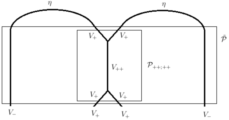
Figure 1: The construction of $\mathcal{P}_{++--}$, follows by composing $\mathcal{P}$ and two invariant pairings ($\eta$).

The RHS of the first line of (86) can be equivariantly mapped to $\mathbb{C}$ by using the invariant pairing between the first $V_{+}$ and first $V_{-}$ and the invariant pairing between second $V_{+}$ and second $V_{-}$. Composing $\tilde{\mathcal{P}}$ with these invariant pairings gives $\mathcal{P}_{++;--}$. We can evaluate this projector on position eigenstates

$$\mathcal{P}_{++--}(e^{-iP\cdot x_{1}}v^{+}\otimes e^{-iP\cdot x_{2}}v^{+}\otimes e^{iK\cdot x_{3}^{\prime}}v^{-}\otimes e^{iK\cdot x_{4}^{\prime}}v^{-})\equiv\mathcal{P}(x_{1},x_{2},x_{3}^{\prime},x_{4}^{\prime})$$ (88)

We can also evaluate it on spherical harmonics

$$\mathcal{P}_{++--}(Y^{l_{1}}_{m_{1}}(P)v^{+}\otimes Y^{l_{2}}_{m_{2}}(P)v^{+}\otimes Y^{l_{3}}_{m_{3}}(K)v^{-}\otimes Y^{l_{4}}_{m_{4}}(K)v^{-})\equiv\mathcal{P}^{l_{1},l_{2},l_{3},l_{4}}_{m_{1},m_{2},m_{3},m_{4}}$$ (89)

Our claim is that the power series expansion of ${1\over 2x_{13}^{2}x_{24}^{2}}F_{1}$ at small $x_{1},x_{2},x_{3}^{\prime},x_{4}^{\prime}$ coincides with that of $\mathcal{P}(x_{1},x_{2},x_{3}^{\prime},x_{4}^{\prime})$

$$\boxed{~{}~{}~{}~{}~{}{1\over 2x_{13}^{2}x_{24}^{2}}F_{1}(u(x_{1},x_{2},x_{3}^{\prime},x_{4}^{\prime}),s(x_{1},x_{2},x_{3}^{\prime},x_{4}^{\prime}))=x_{3}^{\prime 2}x_{4}^{\prime 2}\mathcal{P}(x_{1},x_{2},x_{3}^{\prime},x_{4}^{\prime})~{}~{}~{}~{}~{}~{}}$$ (90)

This is the main result of this section. This power series expansion can be conveniently organised in terms of the coefficients $\mathcal{P}^{l_{1},l_{2},l_{3},l_{4}}_{m_{1},m_{2},m_{3},m_{4}}$.

Consider the coefficient of the product of harmonics in the log term (72). The spherical harmonics $Y^{l}_{m}(x)$ are a basis for harmonic functions regular at $x=0$ and carry a representation of $so(4,2)$. Denote the corresponding function space $H_{+}$. Similarly, $(x^{\prime})^{2}Y^{l}_{m}(x^{\prime})$ are a basis for harmonic functions regular at $x^{\prime}=0$, i.e. $x=\infty$. They also carry a representation of $so(4,2)$. Denote the corresponding function space $H_{-}$. Picking up the coefficient of the harmonics is mapping $H_{+}\otimes H_{+}\otimes H_{-}\otimes H_{-}\rightarrow\mathbb{C}$. This coefficient is just the tensor $C_{l_{1},l_{2},l_{3},l_{4}}^{m_{1},m_{2},m_{3},m_{4}}$ defined in equations (35) and (36) in terms of the structure constants for multiplication of spherical harmonics. The 3-point structure constants involve the integration

$$\int{d^{3}\hat{x}}~{}~{}Y^{l_{1}}_{m_{1}}(\hat{x})Y^{l_{2}}_{m_{2}}(\hat{x})Y^{l_{5}}_{m_{5}}(\hat{x})$$ (91)

Thus picking up the coefficient of $Y^{l_{1}}_{m_{1}}(x_{1})Y^{l_{2}}_{m_{2}}(x_{2})$ involves mapping

$$Y^{l_{1}}_{m_{1}}(x_{1})\otimes Y^{l_{2}}_{m_{2}}(x_{2})\rightarrow r^{l_{1}+l_{2}}Y^{l_{1}}_{m_{1}}(\hat{x})Y^{l_{2}}_{m_{2}}(\hat{x})$$ (92)

$${Y^{l_{3}}_{m_{3}}(x_{3}^{\prime})\over|x_{3}|^{2}}\otimes{Y^{l_{4}}_{m_{4}}(x_{4}^{\prime})\over|x_{4}|^{2}}\rightarrow{Y^{l_{3}}_{m_{3}}(x^{\prime})\over|x|^{2}}\otimes{Y^{l_{4}}_{m_{4}}(x^{\prime})\over|x|^{2}}$$ (93)

These are applications of the equivariant maps $\mathcal{M}:H_{+}\otimes H_{+}\rightarrow H_{++}$ and $\mathcal{M}:H_{-}\otimes H_{-}\rightarrow H_{--}$ as explained in section 5.2 of [32]. From a physical perspective, this corresponds to the fact that the free scalar field $\phi(x)$ has modes transforming in $H_{+}$ (and $H_{-}$) while the field $\phi^{2}(x)$ has modes transforming in $H_{++}$ ( and $H_{--}$). After these maps are applied, the HPEM sets $l_{1}+l_{2}=l+3+l_{4}$ when we do the radial integral and pick up the log term. There remains an integral over $S^{3}$ which gives the factor $(l_{5}+1)^{-1}$. This corresponds, in the discussion of [32] (proposition 84) (see also equation (12) of [43]), to an integral over $U(2)$. Thus we have a direct link between the integration over a modified contour in complexified space-time (where we are integrating over $U(2)$ instead of MInkowski space) and the coefficient of the log term. This is likely to be an example of a general story that should hold for more general Feynman integrals.

We can use the vertex operators of TFT2 to further clarify the discussion. The natural language for the above discussion is in terms of a map $H_{+}\otimes H_{+}\otimes H_{-}\otimes H_{-}\rightarrow\mathbb{C}$. Using the vertex operators we will see that it is equally natural to employ a map $V_{+}\otimes V_{+}\otimes V_{-}\otimes V_{-}\rightarrow\mathbb{C}$. Start with (88) and expand the exponentials in $Y^{l}_{m}(P)Y^{m}_{l}(x)$ or $Y^{l}_{m}(K)Y^{m}_{l}(x^{\prime})$.

$$\sum_{l_{i},m_{i}}{(-i)^{l_{1}}\over 2^{l_{1}}l_{1}!}Y^{l_{1}}_{m_{1}}(x_{1}){(-i)^{l_{2}}\over 2^{l_{2}}l_{2}!}Y^{l_{2}}_{m_{2}}(x_{2}){(i)^{l_{3}}\over 2^{l_{3}}l_{3}!}Y^{l_{3}}_{m_{3}}(x_{3}^{\prime}){(i)^{l_{4}}\over 2^{l_{4}}l_{4}!}Y^{l_{4}}_{m_{4}}(x_{4}^{\prime})$$ (94)

$$\mathcal{P}_{++--}\left(Y_{l_{1}}^{m_{1}}(P)v^{+}\otimes Y_{l_{2}}^{m_{2}}(P)v^{+}\otimes Y_{l_{3}}^{m_{3}}(K)v^{-}\otimes Y_{l_{4}}^{m_{4}}(K)v^{-}\right)$$ (95)

$$=\sum_{l_{i},m_{i}}Y^{l_{1}}_{m_{1}}(x_{1})Y^{l_{2}}_{m_{2}}(x_{2})Y^{l_{3}}_{m_{3}}(x_{3}^{\prime})Y^{l_{4}}_{m_{4}}(x_{4}^{\prime})$$ (96)

$$\mathcal{P}_{++--}\left({Y_{l_{1}}^{m_{1}}(P)\over 2^{l_{1}}l_{1}!}v^{+}\otimes{Y_{l_{2}}^{m_{2}}(P)\over 2^{l_{2}}l_{2}!}v^{+}\otimes{Y_{l_{3}}^{m_{3}}(K)\over 2^{l_{3}}l_{3}!}v^{-}\otimes{Y_{l_{4}}^{m_{4}}(K)\over 2^{l_{4}}l_{4}!}v^{-}\right)$$ (97)

The vertex operators of TFT2 provide equivariant maps between the algebraic state spaces and the polynomial state spaces which makes it possible to express the projector in terms of these state spaces. Indeed, the above argument makes it clear that $\prod Y^{l_{i}}_{m_{i}}(x_{i})$ multiplies a projector acting on states in $V_{+}\otimes V_{+}\otimes V_{-}\otimes V_{-}$. This shows that the claim that the series expansion multiplying the log is the evaluation of an $so(4,2)$ invariant projection on states created from the $v^{\pm}$ by vertex operators, is equivalent to saying that the coefficient of the product of spherical harmonics has to be an equivariant map.

4.1 Analytic consequences

We have seen that the coefficient of the log term in the HPEM has an expansion in powers of $x_{1},x_{2},x_{3}^{\prime},x_{4}^{\prime}$. We will now see how the same expansion arises from the exact answer.

We want to consider the limit $s\rightarrow 0,t\rightarrow 1$, for the conformal cross ratios. It proves to be useful to set $t=1+u$ and then consider $u\rightarrow 0$. The coefficient of $\log s$ is

$$F_{1}={1\over\lambda}\log\left((1+\rho s)\over(1+\rho^{-1}t^{-1})\right)$$ (98)

We can expand this to low powers of $s,u$ using Mathematica, and analysing the results, we arrive at

$$F_{1}(s,u)=\sum_{k=0}^{\infty}{s^{k}\over u^{2k+1}}[Q_{k}(u)\log(1+u)]_{+}$$ (99)

Here $Q_{k}(u)$ is a polynomial in $u$ and $[Q_{k}(u)\log(1+u)]_{+}$ is the truncation of the power series in $u$ to powers $u^{n}$ with $n\geq 2k+1$. $Q_{k}(u)$ is order $k$

$$Q_{k}(u)=\sum_{l=0}^{k}b_{l}(k)u^{l}$$ (100)

where

$$b_{l}(k)={k\choose k-l}{2k+l\choose k-l}$$ (101)

Note that the existence of such an expansion is non-trivial. The individual factors such as $\rho,\lambda,$ when expanded in positive powers of $s$ contain, at each order, a finite number of negative powers of $u$. Nevertheless, the combination of terms appearing in $F_{1}$ is analytic in $u,s$ at $u,s\sim 0$. Appendix B explains how we arrived at the above formula, with the help of Mathematica. The Appendix also explains how the discussion implies a summation formula for products of $su(2)$ Clebsch-Gordan coefficients in terms of $F_{1}$.

5 Quantum Equation of motion, Indecomposable Representations and Equivariant maps

Using the harmonic expansion method, we have found

$$I=I_{1}+I_{2}+I_{3}+I_{4}+I_{5}$$ (102)

$$I=(I_{1;1}^{S}+I_{2;1}^{S})+(I_{2;2}^{S}+I_{3;2}^{S}+I_{3;2}^{L})+(I_{3;3}^{L}+I_{3;3}^{S}+I_{4;3}^{S})+(I_{4;5}^{S}+I_{5;5}^{S})$$ (103)

Rearrange these contributions by defining

$$I^{(1)}=(I_{1;1}^{S}+I_{2;1}^{S})$$ (104)

$$I^{(2)}=(I_{2;2}^{S}+I_{3;2}^{S}+I_{3;2}^{L})$$ (105)

$$I^{(3)}=(I_{3;3}^{L}+I_{3;3}^{S}+I_{4;3}^{S})$$ (106)

$$I^{(4)}=(I_{4;5}^{S}+I_{5;5}^{S})$$ (107)

This reorganization is such that $I^{(i)}$ arises from integration limits where the radial position of the interaction point coincides with the $i$’th external coordinate. In terms of the quantities just introduced, we have

$$I=I^{(1)}+I^{(2)}+I^{(3)}+I^{(4)}$$ (108)

Due to radial ordering, the order of the fields within the correlator swaps when moving from one term to the next. As a consequence of these discontinuities we expect that

$$\boxed{~{}~{}~{}~{}~{}~{}\Box_{j}I^{(i)}=-2\delta_{ij}\prod_{k\neq j}{1\over(x_{k}-x_{i})^{2}}~{}~{}~{}~{}~{}~{}}$$ (109)

We will demonstrate, using the explicit formulae from the HPEM, that this is indeed the case. The $I^{(i)}$ are also used to develop equivariant map interpretations for the full integral $I$. Each $I^{(i)}$ is the starting point for one equivariant map interpretation. We exhibit the complete story for $I^{(1)}$, while the discussion for $I^{(4)}$ is related by inversion. We outline the story for $I^{(2)}$ (and by inversion for $I^{(3)}$). It has an additional intricacy involving the use of a twisted co-product. This raises some technical problems which we leave for the future.

5.1 Quantum equations of motion

Consider the term $I^{(1)}$, which is given by

$$I^{(1)}=\sum_{l_{i},m_{i}}Y^{l_{1}}_{m_{1}}(x_{1}){Y^{l_{2}}_{m_{2}}(x_{2}^{\prime})\over r_{2}^{2}}{Y^{l_{3}}_{m_{3}}(x_{3}^{\prime})\over r_{3}^{2}}{Y^{l_{4}}_{m_{4}}(x_{4}^{\prime})\over r_{4}^{2}}C_{l_{1}l_{2}l_{3}l_{4}}^{m_{1}m_{2}m_{3}m_{4}}{(-2)(l_{1}+1)r_{1}^{2+l_{2}+l_{3}+l_{4}-l_{1}}\over(l_{1}+l_{2}+l_{3}+l_{4}+4)(-l_{1}+l_{2}+l_{3}+l_{4}+2)}$$ (110)

We have written the above formula in terms of a product of harmonic functions in $x_{1},x_{2}^{\prime},x_{3}^{\prime},x_{4}^{\prime}$ so that it has a smooth $x_{1}\rightarrow 0$ limit as well as a smooth $x_{2},x_{3},x_{4}\rightarrow\infty$ limit. To apply the Laplacian, to the above result the formulas

$${\partial^{2}\over\partial x_{1}^{\mu}\partial x_{1}^{\mu}}(r_{1}^{2})^{A}=4A(A+1)(r_{1}^{2})^{A-1}$$ (112)

$${\partial\over\partial x_{1}^{\mu}}(r_{1}^{2})^{A}=2A(r_{1}^{2})^{A-1}x_{1}^{\mu}$$ (113)

$${\partial\over\partial x_{1}^{\mu}}Y^{l_{1}}_{m_{1}}(x_{1}){\partial\over\partial x_{1}^{\mu}}(r_{1}^{2})^{A}=2Al_{1}(r_{1}^{2})^{A-1}Y^{l_{1}}_{m_{1}}(x_{1})$$ (114)

are useful. It is now simple to obtain

$${\partial^{2}\over\partial x_{1}^{\mu}\partial x_{1}^{\mu}}I^{(1)}=\sum_{l_{i},m_{i}}{-2(l_{1}+1)(r_{1})^{l_{2}+l_{3}+l_{4}-l_{1}+2}\over r_{2}^{2}r_{3}^{2}r_{4}^{2}}Y^{l_{1}}_{m_{1}}(x_{1})Y^{l_{2}}_{m_{2}}(x_{2}^{\prime})Y^{l_{3}}_{m_{3}}(x_{3}^{\prime})Y^{l_{4}}_{m_{4}}(x_{4}^{\prime})C_{l_{1}l_{2}l_{3}l_{4}}^{m_{1}m_{2}m_{3}m_{4}}$$ (115)

To recognize the right hand side, note that

$${1\over|x_{1}-x_{2}|^{2}|x_{1}-x_{3}|^{2}|x_{1}-x_{4}|^{2}} ={1\over r_{2}^{2}r_{3}^{2}r_{4}^{2}}\sum_{l_{i},m_{i}}Y^{l_{2}}_{m_{2}}(x_{1})Y^{l_{3}}_{m_{3}}(x_{1})Y^{l_{4}}_{m_{4}}(x_{1})Y^{l_{2}}_{m_{2}}(x_{2}^{\prime})Y^{l_{3}}_{m_{3}}(x_{3}^{\prime})Y^{l_{4}}_{m_{4}}(x_{4}^{\prime})$$ (118)

$$\!\!\!\!\!\!\!\!\!\!\!\!\!\!\!\!\!\!\!\!={(l_{1}+1)r_{1}^{l_{2}+l_{3}+l_{4}}\over r_{2}^{2}r_{3}^{2}r_{4}^{2}}\sum_{l_{i},m_{i}}C_{l_{1}l_{2}l_{3}l_{4}}^{m_{1}m_{2}m_{3}m_{4}}Y^{l_{1}}_{m_{1}}(x)Y^{l_{2}}_{m_{2}}(x_{2}^{\prime})Y^{l_{3}}_{m_{3}}(x_{3}^{\prime})Y^{l_{4}}_{m_{4}}(x_{4}^{\prime})$$

The $(l_{1}+1)$ in the numerator arises because of the normalization of the spherical harmonics. Clearly then, we have demonstrated (109).

The harmonic expansion method expands the propagators in spherical harmonics which solve Laplace’s equation. How then did we get a non-zero answer? The point is that when $|x|<|x_{1}|$ we are expanding in positive powers of $x_{1}^{\prime}$, and when $|x|>|x_{1}|$, we are expanding in positive powers of $x_{1}$. In each case although the $x_{1}$ dependent functions are harmonics, the integration produces an additional dependence on $x_{1}$ from the integration limits. In the operator formalism where we compute a radially ordered correlator the ordering of the interaction vertex changes relative to the external point $x_{1}$ when we move from the region $|x|<|x_{1}|$ to the region $|x|>|x_{1}|$. So, as expected the violation of the free equation has to do with collision of the integration point with an external coordinate.

The contribution $I^{(1)}$ did not include a log dependence. We will consider one more example, $I^{(2)}$, chosen because this term does include a log dependence

$$I^{(2)} = \sum_{l_{i},m_{i}}Y^{l_{1}}_{m_{1}}(x_{1})Y^{l_{2}}_{m_{2}}(x_{2})Y^{l_{3}}_{m_{3}}(x_{3}^{\prime})Y^{l_{4}}_{m_{4}}(x_{4}^{\prime})C_{l_{1}l_{2}l_{3}l_{4}}^{m_{1}m_{2}m_{3}m_{4}}{1\over l_{2}+l_{3}+l_{4}-l_{1}+2}{\delta(l_{1}+l_{2},l_{3}+l_{4})\over r_{3}^{2}r_{4}^{2}}$$

$$+\sum_{l_{i},m_{i}}Y^{l_{1}}_{m_{1}}(x_{1})Y^{l_{2}}_{m_{2}}(x_{2})Y^{l_{3}}_{m_{3}}(x_{3}^{\prime})Y^{l_{4}}_{m_{4}}(x_{4}^{\prime})C_{l_{1}l_{2}l_{3}l_{4}}^{m_{1}m_{2}m_{3}m_{4}}{1\over r_{3}^{2}r_{4}^{2}}$$

$$\times\left[-{r_{2}^{-l_{1}-l_{2}+l_{3}+l_{4}}2(l_{2}+1)\over(l_{2}+l_{3}+l_{4}-l_{1}+2)(l_{3}+l_{4}-l_{1}-l_{2})}(1-\delta(l_{1}+l_{2},l_{3}+l_{4}))-\delta(l_{1}+l_{2},l_{3}+l_{4}){\rm log}(r_{2})\right]$$

We will again make use of the formulas above in (112) as well as

$${\partial\over\partial x_{2}^{\mu}}Y^{l_{2}}_{m_{2}}(x_{2}){\partial\over\partial x_{2}^{\mu}}(r_{2}^{2})^{A}=2Al_{2}(r_{2}^{2})^{A-1}Y^{l_{2}}_{m_{2}}(x_{2})$$ (121)

$${\partial\over\partial x_{2}^{\mu}}{\rm log}r_{2}={x_{2}^{\mu}\over r_{2}^{2}}\qquad\qquad{\partial\over\partial x_{2}^{\mu}}{\partial\over\partial x_{2}^{\mu}}{\rm log}r_{2}={2\over r_{2}^{2}}$$ (122)

We find

$${\partial^{2}\over\partial x_{2}^{\mu}\partial x_{2}^{\mu}}I^{(2)}=-2\sum_{l_{i},m_{i}}(l_{2}+1){r_{2}^{-l_{1}-l_{2}+l_{3}+l_{4}-2}\over r_{3}^{2}r_{4}^{2}}Y^{l_{1}}_{m_{1}}(x_{1})Y^{l_{2}}_{m_{2}}(x_{2})Y^{l_{3}}_{m_{3}}(x_{3}^{\prime})Y^{l_{4}}_{m_{4}}(x_{4}^{\prime})C_{l_{1}l_{2}l_{3}l_{4}}^{m_{1}m_{2}m_{3}m_{4}}$$ (123)

The right hand side can again be identified with

$$-{2\over|x_{1}-x_{2}|^{2}|x_{2}-x_{3}|^{2}|x_{2}-x_{4}|^{2}}$$ (124)

The log contributes the term with $l_{1}+l_{2}=l_{3}+l_{4}$ in (123).

The discussion for the terms $I^{(3)}$ and $I^{(4)}$ is now straight forward.

5.2 QEOM, equivariant maps and their lifts

As we discussed there is an equivariant map between $V_{+}^{(p^{2})}$ and the irrep generated by the field $\phi^{3}$, i.e. the irrep $V_{+++}$ obtained by acting with $(P\cdots P)$ on $v^{+}\otimes v^{+}\otimes v^{+}$. Given the TFT2 construction of free field correlators [13], we know that there is an $so(4,2)$ equivariant map

$${\mathcal{F}}_{1}:V_{+++}\otimes V_{-}\otimes V_{-}\otimes V_{-}\rightarrow\mathbb{C}$$ (125)

such that

$${\mathcal{F}}_{1}(e^{-iP\cdot x_{1}}v_{+++}\otimes e^{iK\cdot x_{2}^{\prime}}v^{-}\otimes e^{iK\cdot x_{3}^{\prime}}v^{-}\otimes e^{iK\cdot x_{4}^{\prime}}v^{-})={x_{2}^{2}x_{3}^{2}x_{4}^{2}\over(x_{1}-x_{2})^{2}(x_{1}-x_{3})^{2}(x_{1}-x_{4})^{2}}$$ (126)

For completeness,we give a derivation in Appendix C. Given the isomorphism between $V_{+}^{(p^{2})}$ and $V_{+++}$, we have a map

$${\mathcal{F}}_{1}:V_{+}^{(p^{2})}\otimes V_{-}\otimes V_{-}\otimes V_{-}\rightarrow\mathbb{C}$$ (127)

It is given similarly by

$${\mathcal{F}}_{1}(e^{-iP\cdot x_{1}}P_{\mu}P_{\mu}v^{+}\otimes e^{iK\cdot x_{2}^{\prime}}v^{-}\otimes e^{iK\cdot x_{3}^{\prime}}v^{-}\otimes e^{iK\cdot x_{4}^{\prime}}v^{-})\!\!\! =~{}{x_{2}^{2}x_{3}^{2}x_{4}^{2}\over(x_{1}-x_{2})^{2}(x_{1}-x_{3})^{2}(x_{1}-x_{4})^{2}}$$ (129)

$$=~{}f(x_{1},x_{2}^{\prime})f(x_{1},x_{3}^{\prime})f(x_{1},x_{4}^{\prime})$$

The function $f(x_{1},x_{2}^{\prime})$ is the series in positive powers of $x_{1},x_{2}^{\prime}$ which sums to

$${1\over(1-2x_{1}\cdot x_{2}^{\prime}+x_{1}^{2}x_{2}^{\prime 2})}$$ (131)

A consistency check of this interpretation is that the Casimirs for each of the four $so(4,2)$’s, one for each coordinate $x_{i}$, gives the value $(-3)$ appropriate for $V_{\pm},\widetilde{V}_{\pm}$ (71).

This map $\mathcal{F}_{1}$ can be lifted from the subspace $V_{+}^{(p^{2})}$ to the larger space $\tilde{V}_{+}$

$$\widetilde{\mathcal{F}}_{1}:\widetilde{V}_{+}\otimes V_{-}\otimes V_{-}\otimes V_{-}\rightarrow\mathbb{C}$$ (132)

Using the relation between algebraic generators $P_{\mu}$ and derivatives in the presence of the vertex operators, this implies

$${\partial^{2}\over\partial x_{1}^{\mu}\partial x_{1}^{\mu}}{\widetilde{\mathcal{F}}_{1}}(e^{-iP\cdot x_{1}}v^{+}\otimes e^{iK\cdot x_{2}^{\prime}}v^{-}\otimes e^{iK\cdot x_{3}^{\prime}}v^{-}\otimes e^{iK\cdot x_{4}^{\prime}}v^{-})=f(x_{1},x_{2}^{\prime})f(x_{1},x_{3}^{\prime})f(x_{1},x_{4}^{\prime})$$ (133)

$\widetilde{\mathcal{F}}_{1}$ is determined by ${\mathcal{F}}_{1}$ up to terms harmonic in $x_{1}$. We know that $x_{2}^{2}x_{3}^{2}x_{4}^{2}I^{(1)}(x_{1},x_{2},x_{3},x_{4})$ solves this differential equation, so we can identify

$$x_{2}^{2}x_{3}^{2}x_{4}^{2}~{}~{}I^{(1)}(x_{1},x_{2},x_{3},x_{4})\rightarrow\widetilde{\mathcal{F}}_{1}(e^{-iP\cdot x_{1}}v^{+}\otimes e^{iK\cdot x_{2}^{\prime}}v^{-}\otimes e^{iK\cdot x_{3}^{\prime}}v^{-}\otimes e^{iK\cdot x_{4}^{\prime}}v^{-})$$ (134)

While $x_{3}^{2}x_{4}^{2}I^{(1)}$ is an $so(4)$-equivariant map, it is not $so(4,2)$ equivariant, even though the Laplacian in $x_{1}$ acting on it gives the $so(4,2)$ equivariant map $\mathcal{F}_{1}$. The equivariance condition under the action of the momentum operator

$$\widetilde{\mathcal{F}}_{1}(P_{\mu}e^{-iP\cdot x_{1}}v^{+}\otimes e^{iK\cdot x_{2}}v^{-}\otimes e^{iK\cdot x_{3}}v^{-}\otimes e^{iK\cdot x_{4}}v^{-})$$ (135)

$$+\widetilde{\mathcal{F}}_{1}(e^{-iP\cdot x_{1}}v^{+}\otimes P_{\mu}e^{iK\cdot x_{2}}v^{-}\otimes e^{iK\cdot x_{3}}v^{-}\otimes e^{iK\cdot x_{4}}v^{-})$$ (136)

$$+\widetilde{\mathcal{F}}_{1}(e^{-iP\cdot x_{1}}v^{+}\otimes e^{iK\cdot x_{2}}v^{-}\otimes P_{\mu}e^{iK\cdot x_{3}}v^{-}\otimes e^{iK\cdot x_{4}}v^{-})$$ (137)

$$+\widetilde{\mathcal{F}}_{1}(e^{-iP\cdot x_{1}}v^{+}\otimes e^{iK\cdot x_{2}}v^{-}\otimes e^{iK\cdot x_{3}}v^{-}\otimes P_{\mu}e^{iK\cdot x_{4}}v^{-})=0$$ (138)

implies that

$$\left({\partial\over\partial x_{1}^{\mu}}+x_{2}^{2}{\partial\over\partial x_{2}^{\mu}}{1\over x_{2}^{2}}+x_{3}^{2}{\partial\over\partial x_{3}^{\mu}}{1\over x_{3}^{2}}+x_{4}^{2}{\partial\over\partial x_{4}^{\mu}}{1\over x_{4}^{2}}\right)\widetilde{\mathcal{F}}_{1}=0$$ (139)

This condition is not satisfied if we identify $\widetilde{\mathcal{F}}_{1}\rightarrow x_{2}^{2}x_{3}^{2}x_{4}^{2}I^{(1)}$. We can add homogeneous terms, annihilated by $\Box_{1}$ to get $x_{2}^{2}x_{3}^{2}x_{4}^{2}(I^{(1)}+I^{(2)}+I^{(3)}+I^{(4)})=x_{2}^{2}x_{3}^{2}x_{4}^{2}I$. Now equivariance under $P_{\mu}$ action of $\widetilde{\mathcal{F}}_{1}$ follows from the standard translation invariance of the integral $I$

$$\left({\partial\over\partial x_{1}^{\mu}}+{\partial\over\partial x_{2}^{\mu}}+{\partial\over\partial x_{3}^{\mu}}+{\partial\over\partial x_{4}^{\mu}}\right)I=0$$ (140)

Similar remarks hold for invariance under the special conformal transformations $K_{\mu}$ and the dilatation operator $D$. Hence the quantum equation of motion along with the requirement of $so(4,2)$ equivariance condition identifies the lift $\widetilde{\mathcal{F}}_{1}$ as

$$\boxed{\widetilde{\mathcal{F}}_{1}(e^{-iP\cdot x_{1}}v^{+}\otimes e^{iK\cdot x_{2}}v^{-}\otimes e^{iK\cdot x_{3}}v^{-}\otimes e^{iK\cdot x_{4}}v^{-})=x_{2}^{2}x_{3}^{2}x_{4}^{2}I(x_{1},x_{2},x_{3},x_{4})={x_{2}^{2}x_{3}^{2}x_{4}^{2}\over x_{13}^{2}x_{24}^{2}}\Phi(s,t)}$$ (141)

By inversion, a similar discussion holds for $I^{(4)}$ and the QEOM for $x_{4}$.

$$\mathcal{F}_{4}:V_{+}\otimes V_{+}\otimes V_{+}\otimes\tilde{V}_{-}\rightarrow\mathbb{C}$$ (142)

with

$$\mathcal{F}_{4}(e^{-iP\cdot x_{1}}v^{+}\otimes e^{-iP\cdot x_{2}}v^{+}\otimes e^{-iP\cdot x_{3}}v^{+}\otimes e^{iK\cdot x_{4}^{\prime}}K_{\mu}K_{\mu}v^{-})={x_{1}^{\prime 2}x_{2}^{\prime 2}x_{3}^{\prime 2}\over(x_{1}^{\prime}-x_{3}^{\prime})^{2}(x_{2}^{\prime}-x_{3}^{\prime})^{2}(x_{3}^{\prime}-x_{4}^{\prime})^{2}}$$ (143)

The $x_{1}^{2}x_{2}^{2}x_{3}^{2}I^{(4)}$ integral is an $so(4)$ invariant lift of $\mathcal{F}_{4}$.

$$\mathcal{F}_{4}(e^{-iP\cdot x_{1}}v^{+}\otimes e^{-iP\cdot x_{2}}v^{+}\otimes e^{-iP\cdot x_{3}}v^{+}\otimes e^{iK\cdot x_{4}^{\prime}}v^{-})\rightarrow x_{1}^{\prime 2}x_{2}^{\prime 2}x_{3}^{\prime 2}~{}~{}I^{(4)}(x_{1},x_{2},x_{3},x_{4})$$ (145)

The $so(4,2)$ equivariant lift is again given by adding homogeneous terms

$$\mathcal{F}_{4}(e^{-iP\cdot x_{1}}v^{+}\otimes e^{-iP\cdot x_{2}}v^{+}\otimes e^{-iP\cdot x_{3}}v^{+}\otimes e^{iK\cdot x_{4}^{\prime}}v^{-})=x_{1}^{\prime 2}x_{2}^{\prime 2}x_{3}^{\prime 2}I(x_{1},x_{2},x_{3},x_{4})$$ (146)

5.3 QEOM and twisted equivariant map

In the above discussion the solution $I^{(1)}$ to the QEOM is not logarithmic. Logarithmic contributions are added to ensure $so(4,2)$ equivariance of the lift from $V_{+}^{(p^{2})}$ to $\widetilde{V}_{+}$. It is interesting to see how things are modified when we consider the case of $I^{(2)}$, which is a logarithmic solution to the quantum equation of motion. It is instructive to consider the free field correlator

$$\langle\phi(x_{1})\phi^{3}(x_{2})\phi(x_{3})\phi(x_{4})\rangle$$ (147)

In the range $|x_{1}|<|x_{2}|<|x_{3}|<|x_{4}|$ relevant to $I^{(2)}$, this free-field correlator, with the correct series expansion, is constructed by taking $\phi^{-}(x_{2}^{\prime})\otimes\phi^{+}(x_{2})\otimes\phi^{+}(x_{2})$ at $x_{2}$ and applying invariant pairings with $\phi^{+}(x_{1})$ and $\phi^{-}(x_{3}^{\prime})\otimes\phi^{-}(x_{4}^{\prime})$. In the free field CFT4/TFT2 construction we used $\phi=\phi^{+}+\phi^{-}$ and the composite field $\phi^{\otimes 3}$ involved sums including $\phi^{+}\otimes\phi^{+}\otimes\phi^{+}$ and $\phi^{-}\otimes\phi^{+}\otimes\phi^{+}$. For such sums to be $so(4,2)$ covariant we must use a twisted co-product.

There is a family of automorphisms of $so(4,2)$ parametrized by a number $\lambda$

$$\alpha_{\lambda}(P_{\mu})={K_{\mu}\over\lambda}\qquad\alpha_{\lambda}(K_{\mu})=\lambda P_{\mu}$$ (148)

$$\alpha_{\lambda}(M_{\mu\nu})=M_{\mu\nu}\qquad\alpha_{\lambda}(D)=-D$$ (149)

A homomorphism between $so(4,2)$ and $so(4,2)^{\otimes 4}$ is given by the twisted co-product

$$\Delta_{\lambda}(\mathcal{L}_{a})=\alpha_{\lambda}(\mathcal{L}_{a})\otimes 1\otimes 1\otimes 1+1\otimes\mathcal{L}_{a}\otimes 1\otimes 1+1\otimes 1\otimes\mathcal{L}_{a}\otimes 1+1\otimes 1\otimes 1\otimes\mathcal{L}_{a}$$ (150)

We can write a new version of (129)

$$\mathcal{F}_{2}(e^{iP\cdot x_{1}}v^{+}\otimes e^{-iP\cdot x_{2}}(P_{\mu}P_{\mu}v^{+})\otimes e^{iK\cdot x_{3}^{\prime}}v^{-}\otimes e^{iK\cdot x_{4}^{\prime}}v^{-})={x_{2}^{2}x_{3}^{2}x_{4}^{2}\over(x_{1}-x_{2})^{2}(x_{2}-x_{3})^{2}(x_{2}-x_{4})^{2}}$$ (151)

where the $so(4,2)$ acts on the tensor product via the above twisted homomorphism, with the choice $\lambda=x_{2}^{2}$. We will express this as

$$\mathcal{F}_{2}:V_{+}^{\prime}\oplus V_{+}^{(p^{2})}\otimes V_{-}\otimes V_{-}\rightarrow\mathbb{C}$$ (152)

The first factor is written as $V_{+}^{\prime}$ because the twist $\alpha_{\lambda}$ is being applied. In the appendix C.2, we show that (151) indeed follows from the equivariance with respect to the twisted co-product. As in the discussion of the $x_{1}$ QEOM above, consider lifts of this map to

$$\tilde{\mathcal{F}}_{2}:V_{+}^{\prime}\oplus\widetilde{V}_{+}\otimes V_{-}\otimes V_{-}\rightarrow\mathbb{C}$$ (153)

In this case converting $P\cdot P$ into a differential operator is quite subtle. This is because there is $x_{2}$ dependence in the vertex operator being inserted at the second slot, but also $x_{2}$ dependence in the twist which determines the map $\widetilde{\mathcal{F}}_{2}$. We will leave the problem of resolving this subtlety as an imporant techincal exercise for the future.

A similar discussion applies to $I^{(3)}$. There is an $so(4,2)$ equivariant map

$$\mathcal{F}_{3}:V_{+}\otimes V_{+}\otimes\widetilde{V}_{-}^{(p^{2})}\otimes V_{-}^{\prime}\rightarrow\mathbb{C}$$ (154)

which gives the RHS of the quantum equation of motion for $x_{3}$. In this case we use a coproduct twisted on the last factor by the automorphism $\alpha_{x_{3}^{\prime 2}}$.

$$\mathcal{F}_{3}(e^{-iP\cdot x_{1}}v^{+}\otimes e^{-iP\cdot x_{2}}v^{+}\otimes K_{\mu}K_{\mu}e^{iK\cdot x_{3}^{\prime}}v^{-}\otimes e^{-iK\cdot x_{4}^{\prime}}v^{-})={x_{1}^{\prime 2}x_{2}^{\prime 2}x_{3}^{\prime 2}\over(x_{1}^{\prime}-x_{3}^{\prime})^{2}(x_{2}^{\prime}-x_{3}^{\prime})^{2}(x_{3}^{\prime}-x_{4}^{\prime})^{2}}$$ (155)

6 Conclusions and Future Directions

Much of our discussion of the four-point integral in four dimensions should generalize to the case of the three-point integral in six dimensions and the six-point integral in three dimensions, when we use the appropriate coordinate space propagators.

6.1 Towards higher loops

We have focused attention on the case of the 1-loop conformal integral. We outline how some key aspects of the discussion generalizes to 2-loops. The 2-loop integral is

$$I_{2}=\int d^{4}x_{5}d^{4}x_{6}{x_{56}^{-2}\over x_{15}^{2}x_{25}^{2}x_{45}^{2}x_{26}^{2}x_{46}^{2}x_{36}^{2}}$$ (157)

where $x_{ij}^{2}=(x_{i}-x_{j})^{2}$. The exact answer is known. It has a term $(\log(s))^{2}F_{2}(s,t)$. The term $F_{2}(s,t)$ can be recovered from the HPEM of integration. Consider the order $|x_{1}|<|x_{2}|<|x_{3}|<|x_{4}|$. This term arises from the integration range $|x_{2}|<|x_{5}|<|x_{6}|<|x_{3}|$. The expansion of the function $F_{2}(s,t)$ has an interpretation in terms of $so(4,2)$ equivariant maps indicated by the diagram in Figure 2.

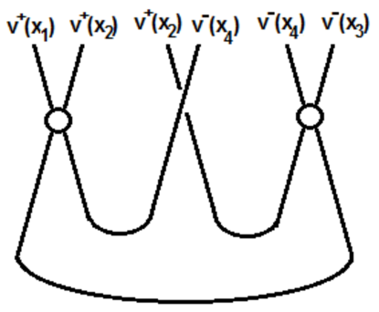
Figure 2: 2-loop conformal integral

It is an equivariant map acting on $e^{-iP\cdot x_{1}}v^{+}\otimes e^{-iP\cdot x_{2}}v^{+}\otimes e^{-iP\cdot x_{2}}v^{+}\otimes e^{iK\cdot x_{3}^{\prime}}v^{-}\otimes e^{iK\cdot x_{3}^{\prime}}v^{-}\otimes e^{iK\cdot x_{4}^{\prime}}v^{-}$. The map is constructed by composing two projectors, one for each integration variable. There is an invariant map pairing two of their indices, corresponding to the internal line. The projectors are the same ones we encountered in the 1-loop discussion $V_{+}\otimes V_{+}\rightarrow V_{++}\rightarrow V_{+}\otimes V_{+}$. It is also possible to modify the diagram, by attaching two external legs to each of $x_{2},x_{4}$ respectively (see Figure 3). In that case, the $x_{2},x_{4}$ become integrated internal vertices. The resulting integral has a fourth power of log which can be recovered from the HPEM method. The coefficient of this logarithmic term is interpreted in terms of a composition of four of the projectors, one for each internal vertex, and is closely related to the coefficient of the log-squared in $I_{2}$.

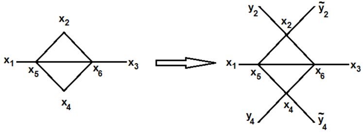
Figure 3: Closely-related-integral

We leave a more careful exposition of the 2-loop and higher loop cases to a forthcoming paper, but the above statements should be fairly plausible to the attentive reader based on the discussion in this paper so far.

6.2 TFT2 and renormalization

The original motivation for this work was to extend free CFT4/TFT2 to interacting theories. The discussion in this paper, developing the relation between Feynman integrals and equivariant maps, gives some useful clues in this direction for the case of perturbative interacting CFTs. Concrete cases to consider are $N=4$ SYM and the Wilson-Fischer fixed point. The connection between quantum equations of motion and indecomposable representations we have described should play a role. In the free CFT4/TFT2, we worked with a state space $\bigoplus Sym^{n}(V_{+}\oplus V_{-})$, where $V_{+}$ is the irreducible representation obtained from $\widetilde{V}_{+}$ by quotienting out the $V_{+}^{(p^{2})}$. For the interacting CFT4, the state space should involve tensor products involving $\widetilde{V}_{+}$ and $\widetilde{V}_{-}$. There will be a coupling dependent quotient given by the quantum equations of motion. Once the correlators are computed at a given order in the perturbation expansion, we know that there is a renormalized formulation where these correlators are reproduced from local operators having dimensions shifted away from their values in the free limit. A TFT2 formulation of perturbative CFT will presumably incorporate this renormalization in a sequence of TFT2s, one for each order of perturbation theory, such that the correlators computed at any stage of the sequence agree with each other. This will embed the renormalization for CFT4s in a TFT2 set-up: the benefit would be to keep, as much as possible, the conformal equivariance properties manifest in the process.

6.3 Conformal blocks and CFT4/TFT2

The existence of a TFT2 approach to CFT4 is made plausible by several known facts about CFT4. CFT4 (and in fact more generally CFT in any dimension) has a distinctively algebraic flavour. By the operator-state correspondence, local operators correspond to definite representations of $so(4,2)$. The spectrum of dimensions in the CFT4 along with the structure constants of the OPE determine the conformal field theory. The description of conformal blocks, which exploits Casimirs in a central way, has a distinct similarity to projectors in representation theory (see for example [34, 35, 36] and more recently in a superconformal setting [52]). While these facts strongly suggest the existence of a TFT2 formulation, the latter is not a trivial consequence. For example, to understand, from a purely representation theoretic point of view (as required in a TFT2 which by definition is about equivariant maps), the fact that the OPE of $\phi^{2}$ with $\phi^{2}$ in the free theory contains $\phi^{2}$ [13] exploits, in an important way, the representation in TFT2 of the quantum field as a linear combination involving both $V_{+}$ and $V_{-}$. The ordinary tensor product of $V_{++}\otimes V_{++}$ does not contain $V_{++}$. An interesting project in the CFT4/TFT2 programme is to understand in terms of equivariant maps, examples in perturbative CFT4 of 4-point functions where factorization involves analogous OPEs, with both the positive dimension representations and their negative dimension duals playing a role.

In special cases of OPEs of the type $\phi^{2}\otimes\phi^{2}\rightarrow\phi^{4}$, where the total number of fields in the intermediate operator is the same as in the external operators, which have a direct analog in the tensor products of positive representations without requiring negative energy representations in a crucial way, there should be a close relation between discussions of conformal blocks in the physics literature [34, 35, 36] and the equivariant map interpretation of integrals developed in [32] .

6.4 HPEM and the interaction/intertwiner connection

The HPEM has been an important tool in our discussion of conformal integrals. It has enabled us to make the connection between $so(4,2)$ equivariant maps involving indecomposable representations and the quantum equations of motion. This connection links a subtle aspect of representation theory with a consequence of the collision of interaction point with external vertex, a deep and generic property of interactions in quantum field theory. Using the HPEM the full integral was decomposed as a sum of terms $I^{(a)}$, each involving the collision of the interaction point with one of the external legs, and each associated with one of the QEOM. It will be very interesting to develop this physical picture for more general Feynman integrals (not necessarily conformal), uncovering the interplay between the collision of interaction points, quantum equations of motion, and equivariance.

As an example of a simple non-conformal integral consider in four dimensions an integration in coordinate space of an $n$-point scalar interaction (with $n\neq 4$). To interpet in terms of $so(4,2)$ equivariance, we would need to combine the scaling in spacetime, with a scaling of the coupling constant. In other words the equivariance would involve a “twisted” $so(4,2)^{\prime}$ which combines the space-time $so(4,2)$ with an $so(2)$ scaling the coupling constant. Twistings which combine space-time symmetries with other symmetries are known to be useful in topological field theories. The idea of employing a scaling of the coupling constant to arrive at a generalized conformal symmetry was developed in [53].

Acknowledgements

SR is supported by STFC Grant ST/J000469/1, String Theory, Gauge Theory, and Duality. RdMK is supported by the South African Research Chairs Initiative of the Department of Science and Technology and the National Research Foundation. We thank Gabriele Travaglini for very useful discussions at various stages of the project. We also thank Andi Brandhuber, Paul Heslop and Donovan Young for useful discussions. SR thanks the Simons summer workshop for hospitality at the Simons Centre for Geometry and Physics, and the Corfu workshop on non-commutative field theory and gravity for hospitality while part of this work was done.

Appendix A Basic formulae for HPEM (harmonic polynomial expansion method)

This Appendix summarizes the formulae used in the harmonic expansion method for integrals. This is also called the Gegenbauer Polynomial expansion technique.

$so(4)$ harmonics : Notation
We will expand the propagators using $so(4)$ spherical harmonics $Y^{l}_{m}(x)$. $x$ is a 4-vector $x^{i}$ in Euclidean space. The positive integer $l$ specifies a symmetric traceless $so(4)$ tensor with rank $l$. We will work with normalization

$${1\over 2\pi^{2}}\int dS^{3}Y^{l_{1}}_{m_{1}}(x)Y^{l_{2}}_{m_{2}}(x)=g_{m_{1}m_{2}}~{}{\delta^{l_{1},l_{2}}\over(l_{1}+1)}$$ (158)

where $dS^{3}$ is the standard metric on the unit sphere. We could work with more general bases where the $g$ factor depends on $l_{1}$, but we won’t use this freedom. One convenient basis is a real orthogonal basis for which

$$g_{m_{1},m_{2}}=\delta_{m_{1},m_{2}}$$ (159)

$$Y_{l}^{m_{1}}(x)=g^{m_{1}m_{2}}Y^{l}_{m_{2}}(x)=Y^{l}_{m_{1}}(x)$$ (160)

$$Y_{l}^{m}(x)=Y^{l}_{m}(x)$$ (161)

Another convenient basis uses the isomorphism $so(4)=su(2)\times su(2)$. A rank $l$ symmetric tensor specifies a representation of spins $({l\over 2},{l\over 2})$. The $so(4)$ state label $m$ is equivalent to a pair of $su(2)$ state labels $(m^{L},m^{R})$ each ranging from $-{l\over 2}$ to ${l\over 2}$. If we work with a basis which diagonalize the $J_{3}^{L},J_{3}^{R}$, then the state label is equivalent to a pair of $su(2)$ labels $(m^{L},m^{R})$

$$g_{m_{1},m_{2}}=\delta_{m_{1},-m_{2}}$$ (162)

$$Y_{l}^{m}(x)=Y^{l}_{-m}(x)$$ (163)

Using the explicit generators $J^{L}_{i},J^{R}_{i}$ given in [13], the charges $(J_{3}^{L},J_{3}^{R})$ for the basic variables are

$$z=x_{1}+ix_{2}\leftrightarrow({1\over 2},{1\over 2})$$ (164)

$$\bar{z}=x_{1}-ix_{2}\leftrightarrow(-{1\over 2},-{1\over 2})$$ (165)

$$w=x_{3}+ix_{4}\leftrightarrow({1\over 2},-{1\over 2})$$ (166)

$$\bar{w}=x_{3}-ix_{4}\leftrightarrow(-{1\over 2},{1\over 2})$$ (167)

We find that

$$Y^{l}_{(l/2,l/2)}=(x_{1}+ix_{2})^{l}=z^{l}$$ (168)

has normalization

$${1\over 2\pi^{2}}\int dS^{3}(Y^{l}_{({l\over 2},{l\over 2})})^{*}~{}~{}Y^{l}_{({l\over 2},{l\over 2})}={1\over(l+1)}$$ (169)

The remaining spherical harmonics are easily generated using the $su(2)$ lowering operators.

Expansion of the exponential vertex operator
The expansion of the exponential in terms of spherical harmonics is

$$e^{-iP\cdot x}v^{+}=\sum_{l,m}{(-i)^{l}\over 2^{l}l!}Y^{l}_{m}(x)Y_{l}^{m}(P)v^{+}$$ (170)

The invariant pairing $\eta:V_{+}\otimes V_{-}\rightarrow\mathbb{C}$ described in terms of harmonics in $P,K$ is

$$\eta\left(Y^{l_{1}}_{m_{1}}(P)v^{+},Y_{l_{2}}^{m_{2}}(K)v^{-}\right)=\delta_{l_{1},l_{2}}\delta_{m_{1},m_{2}}2^{2l_{1}}(l_{1}!)^{2}$$ (171)

The invariant pairing in terms of spherical harmonics in $x$ i.e. $\tilde{\eta}:H_{+}\otimes H_{-}\rightarrow\mathbb{C}$ is

$$\tilde{\eta}\left(Y^{l_{1}}_{m_{1}}(x),{Y_{l_{2}}^{m_{2}}(x^{\prime})\over x^{\prime 2}}\right)=\delta_{l_{1},l_{2}}\delta_{m_{1},m_{2}}$$ (172)

This can be written in terms of integration on the unit 3-sphere [32]

$$\tilde{\eta}\left(Y^{l_{1}}_{m_{1}}(x),{Y_{l_{2}}^{m_{2}}(x^{\prime})\over x^{\prime 2}}\right)={1\over 2\pi^{2}}\int_{S^{3}}{Y_{l_{2}}^{m_{2}}(x^{\prime})\over x^{\prime 2}}(x\cdot\partial_{x}+1)Y^{l_{1}}_{m_{1}}(x))$$ (173)

There are $so(4,2)$ equivariant maps

$$f_{+}:V_{+}\rightarrow H_{-}$$ (174)

$$f_{-}:V_{-}\rightarrow H_{+}$$ (175)

which can be read off from the expansion of the exponential

$$f_{+}:Y^{l}_{m}(P)v^{+}\rightarrow{2^{l}l!}(i)^{l}{Y^{l}_{m}(x^{\prime})\over x^{\prime 2}}$$ (176)

$$f_{-}:Y^{l}_{m}(K)v^{-}\rightarrow{2^{l}l!}(-i)^{l}Y^{l}_{m}(x)$$ (177)

Combining the two maps $f_{+}\otimes f_{-}=f$ gives a map $f:V_{+}\otimes V_{-}\rightarrow H_{-}\otimes H_{+}$. We have $\eta=f\circ\tilde{\eta}$.

Expansion of the 2-point function

$${1\over|\vec{x}-\vec{y}|^{2}} =\sum_{l=0}^{\infty}\sum_{m}{1\over y^{2}}Y^{l}_{m}(x)Y_{l}^{m}(y^{\prime})~{}~{}~{}\hbox{ if}~{}~{}~{}|y|>|x|$$ (179)

$$=\sum_{l=0}^{\infty}\sum_{m}{1\over x^{2}}Y^{l}_{m}(x^{\prime})Y_{l}^{m}(y)~{}~{}~{}\hbox{ if}~{}~{}~{}|x|>|y|$$

Using the addition theorem for spherical harmonics, the RHS can be written in terms of Gegenbauer polynomials of $x\cdot y$. This is a well-known way of doing complicated integrals [45]. We will not be writing expansions in terms of Gegenbauer polynomials, since our main purpose is to keep all four $so(4,2)$’s associated with the external legs manifest, rather than finding an efficient way to do the integrals.

Action of the quadratic $so(4,2)$ Casimir

$$C_{2}=-{1\over 2}L_{MN}L^{MN}=D^{2}-4D+\vec{P}\cdot\vec{K}+{1\over 2}M_{pq}M_{qp}$$ (180)

We will use the differential operator representation of the generators to compute the value of $C_{2}$ when acting on a product of a function of $r$ and a spherical harmonic. As usual, we use vertex operators to obtain the differential opetator corresponding to a particular generator. For example,

$$\vec{P}\cdot\vec{K}e^{-iP\cdot x}v^{+} = P_{p}\left(2ix_{p}x\cdot{\partial\over\partial x}-ix^{2}{\partial\over\partial x_{p}}+2ix_{p}\right)e^{-iP\cdot x}v^{+}$$ (181)

$$= \left(2ix_{p}x\cdot{\partial\over\partial x}-ix^{2}{\partial\over\partial x_{p}}+2ix_{p}\right)i{\partial\over\partial x_{p}}\,\,e^{-iP\cdot x}v^{+}$$ (182)

To obtain the first equality for example, commute $K_{\mu}$ past the vertex operator $e^{-iP\cdot x}$ using the $so(4,2)$ algebra and then use the fact that $K_{\mu}v^{+}=0$. Finally, express the result as a differential operator acting on the vertex operator. Similarly, we find

$$M_{pq}=x_{p}{\partial\over\partial x_{q}}-x_{q}{\partial\over\partial x_{p}}$$ (183)

so that when acting on a power of $r$ times a spherical harmonic we have

$${1\over 2}M_{pq}M_{qp}(r^{A}Y^{l}_{m}(x))={r^{A}\over 2}M_{pq}M_{qp}Y^{l}_{m}(x)=l(l+2)\,r^{A}Y^{l}_{m}(x)$$ (184)

We also have ($D=x\cdot{\partial\over\partial x}+1$ is shifted by 1 to account for the dimension of $v^{+}$)

$$(D^{2}-4D)\,r^{A}Y^{(}x)=[(A+l-2)(A+l)-3]\,r^{A}Y^{l}_{m}(x)$$ (185)

Finally, consider $\vec{P}\cdot\vec{K}$

$$\vec{P}\cdot\vec{K}r^{A}Y^{l}_{m}(x)=(A(A+2)+2Al-2(A+l)^{2})\,r^{A}Y^{l}_{m}(x)$$ (186)

Thus we have

$$C_{2}\,r^{A}Y^{l}_{m}(x)=-3\,r^{A}Y^{l}_{m}(x)$$ (187)

A very similar argument shows that

$$C_{2}\,{\rm log}(r)Y^{l}_{m}(x)=-3\,{\rm log}(r)Y^{l}_{m}(x)$$ (188)

Appendix B Expansion of projector using the exact answer

This section extends the discussion of section 2.2 by providing some of the details behind the expansion. We want to study the limit $s\rightarrow 0,$ $t\rightarrow 1$, i.e. $u\rightarrow 0$ where $t=1+u$. In this limit $\lambda\rightarrow 0$ and $\rho\rightarrow\infty$. The coefficient of the $\log s$ is

$$F_{1}={1\over\lambda}\log\left((1+\rho s)\over(1+\rho^{-1}t^{-1})\right)$$ (189)

Using Mathematica, we expand in $s$ and simplify the function of $u$ appearing at each order of $s$, to obtain

$$F_{1}={\log(1+u)\over u}+{s\over u^{3}}\left(2u-(2+u)\log(1+u)\right)+{s^{2}\over u^{5}}\left(3u(2+u)-6+6u+u^{2})\log(1+u)\right)$$ (190)

$$+{s^{3}\over 3u^{7}}\left(u(60+60u+11u^{2})-3(20+30u+12u^{2}+u^{3})\log(1+u)\right)$$ (191)

After subsequently expanding in powers of $u$, we have

$$F_{1}=\left(-1+{u\over 2}-{u^{2}\over 3}+{u^{3}\over 4}-\cdots\right)+{s}\left({-1\over 6}+{u\over 6}-{3u^{2}\over 20}+\cdots\right)+s^{2}\left({-1\over 30}+{u\over 20}-{2u^{2}\over 35}+\cdots\right)$$ (192)

$$+s^{3}\left({-1\over 140}+{u\over 70}-{5u^{2}\over 252}+\cdots\right)+\cdots$$ (193)

The term at $s^{k}$ is

$${s^{k}\over u^{2k+1}}\left(uP_{k}(u)-Q_{k}(u)\log(1+u)\right)$$ (194)

where $P_{k}(u)$ is a polynomial of degree $k-1$ and $Q_{k}(u)$ is a polynomial of degree $k$, both with positive coefficients. The polynomials have the property that the expansion at $s^{k}$ is regular at $u=0$. In other words

$$uP_{k}(u)-Q_{k}(u)\log(1+u)$$ (195)

only contains powers $u^{n}$ with $n>2k$. This gives $2k+1$ equations constraining the $(2k+1)$ unknown coefficients in $P_{k}$ and $Q_{k}$. These equations do not determine the overall normalization of the two polynomials. This is determined by observing that the leading coefficient in $P_{k}(u)$ is

$${(2k)!\over(k!)^{2}}$$ (196)

which is $(k+1)$ times the $k$’th Catalan number. Writing

$$Q_{k}(u)=\sum_{l=0}^{k}b_{l}u^{l}$$ (197)

we find the linear system of equations

$$\sum_{l=0}^{k}b_{l}{(-1)^{l}\over(i-l)}=0$$ (198)

as $i$ ranges from $k+1$ to $2k$. These come from the requirement that the coefficient of $x^{i}$ vanishes in (195). These equations allow us to solve $b_{1},b_{2},\cdots,b_{k}$ in terms of $b_{0}$. For example, when $k=5$ we have

$$b_{1}={5b_{0}\over 2},\quad b_{2}={20b_{0}\over 9},\quad b_{3}={5b_{0}\over 6},\quad b_{4}={5b_{0}\over 42},\quad b_{5}={b_{0}\over 252}$$ (199)

Interestingly the Catalan number $252$ comes from solving this system of linear equations. To solve (198) for any $k$, define $I=i-k$, where the range of $I$ is $1\leq I\leq k$ and we have

$$\sum_{l=0}^{k}M_{Il}b_{l}=0$$ (200)

where

$$M_{Il}={(-1)^{l}\over(I+k-l)}$$ (201)

The index $l$ ranges over $k+1$ values. We can rewrite (200) as

$$M_{I0}b_{0}=-\sum_{l=1}^{k}M_{Il}b_{l}$$ (202)

Define $\hat{M}_{ab}=M_{ab}$ with $a,b=1,...,k$. Using Mathematica to study a few examples, we have verified that $\hat{M}$ is invertible, so that we can write

$$b_{l}=\sum_{I}\hat{M}^{-1}_{JI}M_{I0}b_{0}$$ (203)

For a specific choice of $k$, it is easy to generate the inverses of $\hat{M}$ in Mathematica and hence to generate the $b_{I}/b_{0}$. For $k=2...7$, we find

$$b_{I}/b_{0}=\{1,1/6\}$$ (204)

$$b_{I}/b_{0}=\{3/2,3/5,1/20\}$$ (205)

$$b_{I}/b_{0}=\{2,9/7,2/7,1/70\}$$ (206)

$$b_{I}/b_{0}=\left\{\frac{5}{2},\frac{20}{9},\frac{5}{6},\frac{5}{42},\frac{1}{252}\right\}$$ (207)

$$b_{I}/b_{0}=\left\{3,\frac{75}{22},\frac{20}{11},\frac{5}{11},\frac{1}{22},\frac{1}{924}\right\}$$ (208)

$$b_{I}/b_{0}=\left\{\frac{7}{2},\frac{63}{13},\frac{175}{52},\frac{175}{143},\frac{63}{286},\frac{7}{429},\frac{1}{3432}\right\}$$ (209)

Using these numerical results from Mathematica and the Online Encyclopaedia of Integer Sequences[54], we find

$$b_{1}(k)/b_{0}=k/2$$ (211)

$$b_{k}(k)/b_{0}={k!^{2}\over(2k)!}$$ (212)

$$b_{k-1}(k)/b_{0}={k!^{2}\over(2k)!}k(k+1)$$ (213)

$$b_{k-2}(k)/b_{0}={k!^{2}\over(2k)!}{(k-1)k(k+1)(k+2)\over 4}$$ (214)

$$b_{k-3}(k)/b_{0}={k!^{2}\over(2k)!}{k\choose 3}{k+3\choose 3}$$ (215)

$$b_{k-m}(k)/b_{0}={k!^{2}\over(2k)!}{k\choose m}{k+m\choose m}$$ (216)

This gives the general formula for the $b$-coefficients. We also know $b_{0}={(2k)!\over k!^{2}}$, so that we have

$$b_{1}(k)=k/2{(2k)!\over k!^{2}}$$ (217)

$$b_{k}(k)=1$$ (218)

$$b_{k-1}(k)=k(k+1)$$ (219)

$$b_{k-2}(k)={(k-1)k(k+1)(k+2)\over 4}$$ (220)

$$b_{k-3}(k)={k\choose 3}{k+3\choose 3}$$ (221)

$$b_{k-m}(k)={k\choose m}{k+m\choose m}$$ (222)

Lets us now consider the polynomial $P_{k}(u)$

$$P_{k}(u)=\sum_{i=1}^{k}a_{i}u^{i-1}$$ (223)

By looking at powers $u^{i}$ in (195) for $1\leq i\leq k$, we obtain the linear equations

$$a_{i}-\sum_{l=0}^{i-1}b_{l}{(-1)^{i-l}\over(i-l)}=0$$ (224)

This gives the $a_{i}$ as sums of binomial coefficients, using the formula for $b$ above. We can again numerically work out the $a$-coefficients for small values of $k$ and then read off the analytic formulas from the patterns we find. For the first few values of $k$ we find

$$k=2:\qquad\vec{a}=\{a_{1},...a_{k}\}=\{6,3\}$$ (225)

$$k=3:\qquad\vec{a}={1\over 3}\times\{60,60,11\}$$ (226)

$$k=4:\qquad\vec{a}={5\over 6}\times\{84,126,52,5\}$$ (227)

$$k=5:\qquad\vec{a}={1\over 30}\times\{7560,15120,9870,2310,137\}$$ (228)

$$k=6:\qquad\vec{a}={7\over 10}\times\{13720,3300,2960,1140,174,7\}$$ (229)

which leads to

$$a_{1}(k)={(2k)!\over(k!)^{2}}$$ (230)

$$a_{k}(k)=2h(k)=2\sum_{l=1}^{k}{1\over l}$$ (231)

$h(k)$ is the k-th harmonic number. Thus, the $a_{i}(k)$ interpolate between Catalan numbers and harmonic numbers. In this way, the Catalan numbers, along with the form (194), has determined all the coefficients in the double Taylor expansion around $s,u=0$.

B.1 A summation formula for products of $su(2)$ Clebschs from Feynman Integrals

Our discussion implies a summation formula for products of $su(2)$-Clebsh Gordan coefficients, since these coefficients appear in the multiplication of spherical harmonics which enter the definition of the $so(4,2)$ equivariant map $\mathcal{M}$. Indeed, equating the result for the coefficient of the log obtained from HPEM to the coefficient of the same log appearing in the exact result, we have

$$\boxed{\begin{aligned} ~{}~{}~{}~{}&\sum_{l_{i}=0}^{\infty}\sum_{m_{i}}\sum_{t=0}^{\infty}\sum_{p}\delta_{l_{1}+l_{2},l_{3}+l_{4}}Y^{l_{1}}_{-m_{1}}(x_{1})Y^{l_{2}}_{-m_{2}}(x_{2})Y^{l_{3}}_{m_{3}}(x^{\prime}_{3})Y^{l_{4}}_{m_{4}}(x^{\prime}_{4})\times{C^{{l_{1}},{l_{2}};{t}}_{m_{1},m_{2};p}C^{l_{3},l_{4};t}_{-m_{3},-m_{4};-p}\over t+1}~{}~{}~{}~{}\\ &\qquad={x_{3}^{2}x_{4}^{2}\over x_{13}^{2}x_{24}^{2}}{1\over\lambda}\log\left((1+\rho s)\over(1+\rho^{-1}t^{-1})\right)~{}~{}~{}~{}~{}\end{aligned}}\\$$ (232)

Noting that the structure constants of the multiplication of $so(4)$-covariant harmonics on $S^{3}$ can be written in terms of Clebsch-Gordan coefficients of $su(2)$

$${{C^{~{}l_{1},~{}l_{2}~{};~{}~{}~{}l}_{m_{1},m_{2}~{};~{}m_{1}+m_{2}}}}=\left\langle\begin{tabular}[]{cc}${l_{1}\over 2}$&${l_{2}\over 2}$\\ ${m_{1}^{L}\over 2}$&${m_{2}^{L}\over 2}$\end{tabular}\Bigg{|}\begin{tabular}[]{c}${l\over 2}$\\ ${m_{1}^{L}+m_{2}^{L}\over 2}$\end{tabular}\right\rangle\left\langle\begin{tabular}[]{cc}${l_{1}\over 2}$&${l_{2}\over 2}$\\ ${m_{1}^{R}\over 2}$&${m_{2}^{R}\over 2}$\end{tabular}\Bigg{|}\begin{tabular}[]{c}${l\over 2}$\\ ${m_{1}^{R}+m_{2}^{R}\over 2}$\end{tabular}\right\rangle$$

we see that (232) is a highly nontrivial sum rule for $su(2)$-Clebsh Gordan coefficients.

To check this sum rule, it is useful to use the basis which diagonalizes the $(J_{3}^{L},J_{3}^{R})$ sub-algebra of $su(2)\times su(2)$, described in (167). Using this basis we can easily determine the coefficients of monomials of a specific form appearing on both side of (232). The simplest monomial arises from the terms in the sum with $t=0$ and

$$Y^{{n_{1}\over 2}}_{{n_{1}\over 2},{n_{1}\over 2}}(x_{1})Y^{{n_{2}\over 2}}_{{n_{2}\over 2},{n_{2}\over 2}}(x_{2})Y^{{n_{3}\over 2}}_{{-n_{3}\over 2},{-n_{3}\over 2}}(x_{1})Y^{{n_{4}\over 2}}_{{-n_{4}\over 2},{-n_{4}\over 2}}(x_{4})=z_{1}^{n_{1}}z_{2}^{n_{2}}\bar{z}_{3}^{n_{3}}\bar{z}_{4}^{n_{4}}$$ (233)

In this extremal case, the Clebsch Gordan coefficients are 1, so that the monomial $z_{1}^{n_{1}}z_{2}^{n_{2}}\bar{z}_{3}^{n_{3}}\bar{z}_{4}^{n_{4}}$ has coefficient ${1\over n_{1}+n_{2}+1}$. To recover this coefficient from the RHS of (232), note that

$$(x_{i}-x_{j})^{2} = 1-2x_{i}\cdot x_{j}+x_{i}^{2}x_{j}^{2}$$ (234)

$$= 1-z_{i}\bar{z}_{j}-\bar{z}_{i}z_{j}-w_{i}\bar{w}_{j}-\bar{w}_{i}w_{j}+(z_{i}\bar{z}_{i}+w_{i}\bar{w}_{i})(z_{j}\bar{z}_{j}+w_{j}\bar{w}_{j})$$ (235)

Inserting this into the RHS of (232) and expanding as described at the start of this Appendix, we can obtain the coefficient of any given monomial. In particular, we verify that $z_{1}^{n_{1}}z_{2}^{n_{2}}\bar{z}_{3}^{n_{3}}\bar{z}_{4}^{n_{4}}$ has coefficient ${1\over n_{1}+n_{2}+1}$. Next consider

$$Y^{n_{1}\over 2}_{{n_{1}\over 2},{n_{1}-2\over 2}}(x_{1})Y^{n_{2}\over 2}_{{n_{2}-2\over 2},{n_{2}\over 2}}(x_{2})Y^{n_{3}\over 2}_{-{n_{3}\over 2},-{n_{3}-2\over 2}}(x_{3})Y^{n_{4}\over 2}_{-{n_{4}-2\over 2},-{n_{4}\over 2}}(x_{4})$$ (236)

(237)

$$=\sqrt{n_{1}n_{2}n_{3}n_{4}}z_{1}^{n_{1}-1}\bar{w}_{1}z_{2}^{n_{2}-1}w_{2}\bar{z}_{3}^{n_{3}-1}w_{3}\bar{z}_{4}^{n_{4}-1}\bar{w}_{4}$$ (238)

which invloves terms in the sum with $t=0$ and $t=1$. We need two Clebsch Gordan coefficients

$$C^{{n_{1}\over 2},{n_{2}\over 2},{n_{1}+n_{2}\over 2}}_{\left({n_{1}\over 2},{n_{1}-2\over 2}\right),\left({n_{2}-2\over 2},{n_{2}\over 2}\right),\left({n_{1}+n_{2}-2\over 2},{n_{1}+n_{2}-2\over 2}\right)}={\sqrt{n_{1}n_{2}}\over n_{1}+n_{2}}$$ (239)

$$C^{{n_{1}\over 2},{n_{2}\over 2},{n_{1}+n_{2}-2\over 2}}_{\left({n_{1}\over 2},{n_{1}-2\over 2}\right),\left({n_{2}-2\over 2},{n_{2}\over 2}\right),\left({n_{1}+n_{2}-2\over 2},{n_{1}+n_{2}-2\over 2}\right)}={\sqrt{n_{1}n_{2}}\over n_{1}+n_{2}}$$ (240)

which easily follow from the following $su(2)$ coefficients

$$C^{{n_{1}\over 2},{n_{2}\over 2},{n_{1}+n_{2}\over 2}}_{{n_{1}\over 2},{n_{2}-2\over 2},{n_{1}+n_{2}-2\over 2}}=\sqrt{n_{2}\over n_{1}+n_{2}}$$ (241)

$$C^{{n_{1}\over 2},{n_{2}\over 2},{n_{1}+n_{2}-2\over 2}}_{{n_{1}\over 2},{n_{2}-2\over 2},{n_{1}+n_{2}-2\over 2}}=-\sqrt{n_{1}\over n_{1}+n_{2}}$$ (242)

Explicit formulae for the $su(2)$ Clebsch Gordan coefficients are available in [55]. Thus, the coefficient of $z_{1}^{n_{1}-1}\bar{w}_{1}z_{2}^{n_{2}-1}w_{2}\bar{z}_{3}^{n_{3}-1}w_{3}\bar{z}_{4}^{n_{4}-1}\bar{w}_{4}$ is

$$\sqrt{n_{1}n_{2}n_{3}n_{4}}\left[C^{{n_{1}\over 2},{n_{2}\over 2},{n_{1}+n_{2}\over 2}}_{\left({n_{1}\over 2},{n_{1}-2\over 2}\right),\left({n_{2}-2\over 2},{n_{2}\over 2}\right),\left({n_{1}+n_{2}-2\over 2},{n_{1}+n_{2}-2\over 2}\right)}{1\over n_{1}+n_{2}+1}\right.$$ (243)

$$\left.+C^{{n_{1}\over 2},{n_{2}\over 2},{n_{1}+n_{2}-2\over 2}}_{\left({n_{1}\over 2},{n_{1}-2\over 2}\right),\left({n_{2}-2\over 2},{n_{2}\over 2}\right),\left({n_{1}+n_{2}-2\over 2},{n_{1}+n_{2}-2\over 2}\right)}{1\over n_{1}+n_{2}}\right]$$ (244)

$$={2n_{1}n_{2}n_{3}n_{4}\over(n_{1}+n_{2}-1)(n_{1}+n_{2})(n_{1}+n_{2}+1)}$$ (245)

This again agrees with the coefficient obtained by expanding the RHS of (232).

Appendix C Equivariant maps related to Quantum Equations of Motion

This section gives the explicit evaluation of the maps $\mathcal{F}_{1}$ and $\mathcal{F}_{2}$ which are introduced in section 5.

C.1 Quantum equation of motion for $x_{1}$

When we evaluate the map $\mathcal{F}_{1}$ with the exponential states inserted, we get an expression which has a well defined expansion at small $x_{1},x_{2}^{\prime},x_{3}^{\prime},x_{4}^{\prime}$. Set $h(x_{1},x_{2}^{\prime},x_{3}^{\prime},x_{4}^{\prime})={\mathcal{F}}_{1}(e^{-iP\cdot x_{1}}v^{+++}\otimes e^{iK\cdot x_{2}^{\prime}}v^{-}\otimes e^{iK\cdot x_{3}^{\prime}}v^{-}\otimes e^{iK\cdot x_{4}^{\prime}}v^{-})$. Then

$${\partial h\over\partial x^{\mu}_{1}} = -i\mathcal{F}_{1}(P_{\mu}e^{-iP\cdot x_{1}}v^{+++}\otimes e^{iK\cdot x_{2}^{\prime}}v^{-}\otimes e^{iK\cdot x_{3}^{\prime}}v^{-}\otimes e^{iK\cdot x_{4}^{\prime}}v^{-})$$ (246)

$$= i{\mathcal{F}}_{1}(e^{-iP\cdot x_{1}}v^{+++}\otimes P_{\mu}e^{iK\cdot x_{2}^{\prime}}v^{-}\otimes e^{iK\cdot x_{3}^{\prime}}v^{-}\otimes e^{iK\cdot x_{4}^{\prime}}v^{-})$$ (249)

$$+i{\mathcal{F}}_{1}(e^{-iP\cdot x_{1}}v^{+++}\otimes e^{iK\cdot x_{2}^{\prime}}v^{-}\otimes P_{\mu}e^{iK\cdot x_{3}^{\prime}}v^{-}\otimes e^{iK\cdot x_{4}^{\prime}}v^{-})$$

$$+i{\mathcal{F}}_{1}(e^{-iP\cdot x_{1}}v^{+++}\otimes e^{iK\cdot x_{2}^{\prime}}v^{-}\otimes e^{iK\cdot x_{3}^{\prime}}v^{-}\otimes P_{\mu}e^{iK\cdot x_{4}^{\prime}}v^{-})$$

where the last line follows from the $so(4,2)$ invariance of $\mathcal{F}_{1}$. Now,

$$P_{\mu}e^{iK\cdot x_{3}^{\prime}}v^{-} = \left(2ix_{3\mu}^{\prime}x_{3}^{\prime}\cdot{\partial\over\partial x_{3}^{\prime}}-ix_{3}^{\prime 2}{\partial\over\partial x_{3\mu}^{\prime}}+2ix_{3\mu}^{\prime}\right)e^{iK\cdot x_{3}^{\prime}}v^{-}$$ (250)

$$= ix_{3}^{2}\,\,{\partial\over\partial x_{3}^{\mu}}\,\,{1\over x_{3}^{2}}e^{iK\cdot x_{3}^{\prime}}v^{-}$$ (251)

so that (249) becomes

$${\partial h\over\partial x^{\mu}_{1}} = -x_{2}^{2}\,\,{\partial\over\partial x_{2}^{\mu}}\,\,({1\over x_{2}^{2}}h)-x_{3}^{2}\,\,{\partial\over\partial x_{3}^{\mu}}\,\,({1\over x_{3}^{2}}h)-x_{4}^{2}\,\,{\partial\over\partial x_{4}^{\mu}}\,\,({1\over x_{4}^{2}}h)$$ (252)

which can be written as

$$x_{2}^{2}x_{3}^{2}x_{4}^{2}\left({\partial\over\partial x_{1}^{\mu}}+{\partial\over\partial x_{2}^{\mu}}+{\partial\over\partial x_{3}^{\mu}}+{\partial\over\partial x_{4}^{\mu}}\right)\left[{h\over x_{2}^{2}x_{3}^{2}x_{4}^{2}}\right]=0$$ (253)

This proves the map is only a function of the differences $x_{i}^{\mu}-x_{j}^{\mu}$. Next, consider

$$\left(x_{1\mu}{\partial\over\partial x_{1\nu}}-x_{1\nu}{\partial\over\partial x_{1\mu}}\right)h = \mathcal{F}_{1}(M_{\mu\nu}e^{-iP\cdot x_{1}}v^{+++}\otimes e^{iK\cdot x_{2}^{\prime}}v^{-}\otimes e^{iK\cdot x_{3}^{\prime}}v^{-}\otimes e^{iK\cdot x_{4}^{\prime}}v^{-})$$ (254)

$$= -{\mathcal{F}}_{1}(e^{-iP\cdot x_{1}}v^{+++}\otimes M_{\mu\nu}e^{iK\cdot x_{2}^{\prime}}v^{-}\otimes e^{iK\cdot x_{3}^{\prime}}v^{-}\otimes e^{iK\cdot x_{4}^{\prime}}v^{-})$$ (255)

$$- {\mathcal{F}}_{1}(e^{-iP\cdot x_{1}}v^{+++}\otimes e^{iK\cdot x_{2}^{\prime}}v^{-}\otimes M_{\mu\nu}e^{iK\cdot x_{3}^{\prime}}v^{-}\otimes e^{iK\cdot x_{4}^{\prime}}v^{-})$$ (256)

$$- {\mathcal{F}}_{1}(e^{-iP\cdot x_{1}}v^{+++}\otimes e^{iK\cdot x_{2}^{\prime}}v^{-}\otimes e^{iK\cdot x_{3}^{\prime}}v^{-}\otimes M_{\mu\nu}e^{iK\cdot x_{4}^{\prime}}v^{-})$$ (257)

which after a little algebra can be written as

$$x_{2}^{2}x_{3}^{2}x_{4}^{2}\left(x_{1\mu}{\partial\over\partial x_{1\nu}}-x_{1\nu}{\partial\over\partial x_{1\mu}}+x_{2\mu}{\partial\over\partial x_{2\nu}}-x_{2\nu}{\partial\over\partial x_{2\mu}}+x_{3\mu}{\partial\over\partial x_{3\nu}}-x_{3\nu}{\partial\over\partial x_{3\mu}}\right.$$ (258)

$$\left.+x_{4\mu}{\partial\over\partial x_{4\nu}}-x_{4\nu}{\partial\over\partial x_{4\mu}}\right)\left[{h\over x_{2}^{2}x_{3}^{2}x_{4}^{2}}\right]=0$$ (259)

This proves the map is only a function of the magnitudes of the differences $|x_{i}^{\mu}-x_{j}^{\mu}|$. Next, consider

$$\left(x_{1}\cdot{\partial\over\partial x_{1}}+3\right)h = \mathcal{F}_{1}(e^{-iP\cdot x_{1}}v^{+++}\otimes e^{iK\cdot x_{2}^{\prime}}v^{-}\otimes e^{iK\cdot x_{3}^{\prime}}v^{-}\otimes e^{iK\cdot x_{4}^{\prime}}v^{-})$$ (260)

$$= -\mathcal{F}_{1}(e^{-iP\cdot x_{1}}v^{+++}\otimes De^{iK\cdot x_{2}^{\prime}}v^{-}\otimes e^{iK\cdot x_{3}^{\prime}}v^{-}\otimes e^{iK\cdot x_{4}^{\prime}}v^{-})$$ (261)

$$- \mathcal{F}_{1}(e^{-iP\cdot x_{1}}v^{+++}\otimes e^{iK\cdot x_{2}^{\prime}}v^{-}\otimes De^{iK\cdot x_{3}^{\prime}}v^{-}\otimes e^{iK\cdot x_{4}^{\prime}}v^{-})$$ (262)

$$- \mathcal{F}_{1}(e^{-iP\cdot x_{1}}v^{+++}\otimes e^{iK\cdot x_{2}^{\prime}}v^{-}\otimes e^{iK\cdot x_{3}^{\prime}}v^{-}\otimes De^{iK\cdot x_{4}^{\prime}}v^{-})$$ (263)

This can be rewritten as

$$x_{2}^{2}x_{3}^{2}x_{4}^{2}\left(x_{1}\cdot{\partial\over\partial x_{1}}+x_{2}\cdot{\partial\over\partial x_{2}}+x_{3}\cdot{\partial\over\partial x_{3}}+x_{4}\cdot{\partial\over\partial x_{4}}+12\right)\left[{h\over x_{2}^{2}x_{3}^{2}x_{4}^{2}}\right]=0$$ (264)

This tells us the degree of the dependence on $|x_{i}^{\mu}-x_{j}^{\mu}|$. Thus, at this stage we know that

$${h\over x_{2}^{2}x_{3}^{2}x_{4}^{2}}={A\over|x_{1}-x_{2}|^{2\alpha}|x_{1}-x_{3}|^{2\beta}|x_{1}-x_{4}|^{2\gamma}|x_{2}-x_{3}|^{2\delta}|x_{2}-x_{4}|^{2\eta}|x_{3}-x_{4}|^{2\tau}}$$ (265)

and $\alpha+\beta+\gamma+\delta+\eta+\tau=6$. Thus, the map has now been reduced to determining 7 numbers. To determine these numbers start by noting that at $x_{1}=0$ and $x_{2}^{\prime}=x_{3}^{\prime}=x_{4}^{\prime}=0$ we have

$$h(0,0,0,0)=\mathcal{F}_{1}(v^{+++}\otimes v^{-}\otimes v^{-}\otimes v^{-})=1$$ (266)

i.e. $h$ has no singularities and takes the constant value 1. This implies that $\delta=\eta=\tau=0$, $\alpha=\beta=\gamma=1$ and $A=1$, which proves (126).

C.2 Quantum equation of motion for $x_{2}$

Using invariance of the map and the $so(4,2)$ algebra,we can easily prove (151). Towards this end, recall some results which follow from the invariant pairing

$$\eta(e^{-iP\cdot x_{1}}v^{+},e^{iK\cdot x_{2}^{\prime}}v^{-})=\sum_{n,m=0}^{\infty}{i^{m}(-1)^{n}\over n!m!}x_{1}^{\alpha_{1}}\cdots x_{1}^{\alpha_{n}}x_{2}^{\prime\beta_{1}}\cdots x_{2}^{\prime\beta_{m}}T_{\alpha_{1}\cdots\alpha_{n}\beta_{1}\cdots\beta_{m}}$$ (267)

where

$$T_{\alpha_{1}\cdots\alpha_{n}\beta_{1}\cdots\beta_{m}} = \eta(P_{\alpha_{1}}\cdots P_{\alpha_{n}}v^{+},K_{\beta_{1}}\cdots K_{\beta_{m}}v^{-})$$ (268)

$$= (-1)^{n}\eta(v^{+},P_{\alpha_{n}}\cdots P_{\alpha_{1}}K_{\beta_{1}}\cdots K_{\beta_{m}}v^{-})$$ (269)

$$= (-1)^{m}\eta(K_{\beta_{m}}\cdots K_{\beta_{1}}P_{\alpha_{1}}\cdots P_{\alpha_{n}}v^{+},v^{-})$$ (270)

and the last two lines above follow from the $so(4,2)$ invariance of the pairing. Now, setting

$$K_{\beta_{m}}\cdots K_{\beta_{1}}P_{\alpha_{1}}\cdots P_{\alpha_{n}}v^{+}=\delta_{nm}t_{\alpha_{1}\cdots\alpha_{n}\beta_{1}\cdots\beta_{m}}v^{+}$$ (271)

$$P_{\alpha_{n}}\cdots P_{\alpha_{1}}K_{\beta_{1}}\cdots K_{\beta_{m}}v^{-}=\delta_{nm}t_{\alpha_{1}\cdots\alpha_{n}\beta_{1}\cdots\beta_{m}}v^{-}$$ (272)

we find

$$T_{\alpha_{1}\cdots\alpha_{n}\beta_{1}\cdots\beta_{m}}=t_{\alpha_{1}\cdots\alpha_{n}\beta_{1}\cdots\beta_{m}}(-1)^{m}$$ (273)

and

$$\sum_{n=0}^{\infty}{(-1)^{n}\over n!m!}x_{1}^{\alpha_{1}}\cdots x_{1}^{\alpha_{n}}x_{2}^{\prime\beta_{1}}\cdots x_{2}^{\prime\beta_{n}}t_{\alpha_{1}\cdots\alpha_{n}\beta_{1}\cdots\beta_{n}}={1\over 1-2x_{2}^{\prime}\cdot x_{1}+x_{1}^{2}x_{2}^{\prime 2}}$$ (274)

We will make use of (271), (272) and (274) below. Consider the complete expansion

$$\mathcal{F}_{2}(e^{iP\cdot x_{1}}v^{+}\otimes e^{-iP\cdot x_{2}}v^{+++}\otimes e^{iK\cdot x_{3}^{\prime}}v^{-}\otimes e^{iK\cdot x_{4}^{\prime}}v^{-})$$ (275)

$$= \sum_{n_{1},n_{3},n_{4}=0}^{\infty}{1\over n_{1}!n_{3}!n_{4}!}\mathcal{F}_{2}((iP\cdot x_{1})^{n_{1}}v^{+}\otimes e^{-iP\cdot x_{2}}v^{+++}\otimes(iK\cdot x_{3}^{\prime})^{n_{3}}v^{-}\otimes(iK\cdot x_{4}^{\prime})^{n_{4}}v^{-})$$ (276)

Expand the remaining exponential and use equivariance of the map to transfer the $P\cdot x_{2}$ factors into the other three slots. Due to the twisting, when we move $P\cdot x_{2}$ into the first slot we get

$$\alpha(P\cdot x_{2})={1\over x_{2}^{2}}K\cdot x_{2}=K\cdot x_{2}^{\prime}$$ (278)

For a given term in the sum (i.e. a given $n_{1},n_{3},n_{3}$) only a specific power of $P\cdot x_{2}$ from the expansion of the exponential in slot 2 will contribute. Keeping only this power we have

$$\mathcal{F}_{2}(e^{iP\cdot x_{1}}v^{+}\otimes e^{-iP\cdot x_{2}}v^{+++}\otimes e^{iK\cdot x_{3}^{\prime}}v^{-}\otimes e^{iK\cdot x_{4}^{\prime}}v^{-})$$ (279)

$$= \sum_{n_{1},n_{3},n_{4}=0}^{\infty}{1\over n_{1}!n_{3}!n_{4}!(n_{1}+n_{3}+n_{4})!}$$ (281)

$$\times\mathcal{F}_{2}((iP\cdot x_{1})^{n_{1}}v^{+}\otimes(-iP\cdot x_{2})^{n_{1}+n_{3}+n_{4}}v^{+++}\otimes(iK\cdot x_{3}^{\prime})^{n_{3}}v^{-}\otimes(iK\cdot x_{4}^{\prime})^{n_{4}}v^{-})$$

$$= \sum_{n_{1},n_{3},n_{4}=0}^{\infty}{1\over n_{1}!n_{3}!n_{4}!(n_{1}+n_{3}+n_{4})!}{(n_{1}+n_{3}+n_{4})!\over n_{1}!n_{3}!n_{4}!}(-1)^{n_{1}+n_{3}+n_{4}}$$ (284)

$$\times\mathcal{F}_{2}((\alpha(P\cdot x_{2}))^{n_{1}}(P\cdot x_{1})^{n_{1}}v^{+}\otimes v^{+++}\otimes(P\cdot x_{2})^{n_{3}}(K\cdot x_{3}^{\prime})^{n_{3}}v^{-}\otimes(P\cdot x_{2})^{n_{4}}(K\cdot x_{4}^{\prime})^{n_{4}}v^{-})$$

$$= \sum_{n_{1}}^{\infty}{(-1)^{n_{1}}\over(n_{1}!)^{2}}x_{1}^{\alpha_{1}}\cdots x_{1}^{\alpha_{n_{1}}}x_{2}^{\prime\beta_{1}}\cdots x_{2}^{\prime\beta_{n_{1}}}t_{\alpha_{1}\cdots\alpha_{n_{1}}\beta_{1}\cdots\beta_{n_{1}}}$$ (288)

$$\times\,\sum_{n_{3}}^{\infty}{(-1)^{n_{3}}\over(n_{1}!)^{2}}x_{2}^{\gamma_{1}}\cdots x_{2}^{\gamma_{n_{3}}}x_{3}^{\prime\delta_{1}}\cdots x_{3}^{\prime\delta_{n_{3}}}t_{\gamma_{1}\cdots\gamma_{n_{3}}\delta_{1}\cdots\delta_{n_{3}}}$$

$$\times\sum_{n_{4}}^{\infty}{(-1)^{n_{4}}\over(n_{1}!)^{2}}x_{2}^{\mu_{1}}\cdots x_{2}^{\mu_{n_{4}}}x_{4}^{\prime\nu_{1}}\cdots x_{4}^{\prime\nu_{n_{4}}}t_{\mu_{1}\cdots\mu_{n_{4}}\nu_{1}\cdots\nu_{n_{4}}}\mathcal{F}_{2}(v^{+}\otimes v^{+++}\otimes v^{-}\otimes v^{-})$$

$$= {1\over 1-2x_{1}\cdot x_{2}^{\prime}+x_{1}^{2}x_{2}^{\prime 2}}{1\over 1-2x_{2}\cdot x_{3}^{\prime}+x_{2}^{2}x_{3}^{\prime 2}}{1\over 1-2x_{2}\cdot x_{4}^{\prime}+x_{2}^{2}x_{4}^{\prime 2}}$$ (290)

$$= {x_{2}^{2}x_{3}^{3}x_{4}^{2}\over(x_{1}-x_{2})^{2}(x_{2}-x_{3})^{2}(x_{2}-x_{4})^{2}}$$ (292)

which proves the result (151).

References

- [1] R. de Mello Koch and S. Ramgoolam, “Strings from Feynman Graph counting : without large N,” Phys. Rev. D 85 (2012) 026007 [arXiv:1110.4858 [hep-th]].
- [2] R. de Mello Koch, S. Ramgoolam and C. Wen, “On the refined counting of graphs on surfaces,” Nucl. Phys. B 870 (2013) 530 [arXiv:1209.0334 [hep-th]].
- [3] J. Pasukonis and S. Ramgoolam, “Quivers as Calculators: Counting, Correlators and Riemann Surfaces,” JHEP 1304 (2013) 094 [arXiv:1301.1980 [hep-th]].
- [4] Y. Kimura, “Multi-matrix models and Noncommutative Frobenius algebras obtained from symmetric groups and Brauer algebras,” Commun. Math. Phys. 337 (2015) 1, 1 [arXiv:1403.6572 [hep-th]].
- [5] V. Jejjala, S. Ramgoolam and D. Rodriguez-Gomez, “Toric CFTs, Permutation Triples and Belyi Pairs,” JHEP 1103 (2011) 065 [arXiv:1012.2351 [hep-th]].
- [6] T. W. Brown, “Complex matrix model duality,” Phys. Rev. D 83 (2011) 085002 [arXiv:1009.0674 [hep-th]].
- [7] S. Corley, A. Jevicki and S. Ramgoolam, “Exact correlators of giant gravitons from dual N=4 SYM theory,” Adv. Theor. Math. Phys. 5 (2002) 809 [hep-th/0111222].
- [8] R. d. M. Koch, M. Dessein, D. Giataganas and C. Mathwin, “Giant Graviton Oscillators,” JHEP 1110 (2011) 009 [arXiv:1108.2761 [hep-th]].
- [9] R. de Mello Koch and S. Ramgoolam, “A double coset ansatz for integrability in AdS/CFT,” JHEP 1206 (2012) 083 [arXiv:1204.2153 [hep-th]].
- [10] J. Ben Geloun and S. Ramgoolam, “Counting Tensor Model Observables and Branched Covers of the 2-Sphere,” arXiv:1307.6490 [hep-th].
- [11] J. A. Minahan and K. Zarembo, “The Bethe ansatz for N=4 superYang-Mills,” JHEP 0303 (2003) 013 [hep-th/0212208].
- [12] N. Beisert, C. Kristjansen and M. Staudacher, “The Dilatation operator of conformal N=4 superYang-Mills theory,” Nucl. Phys. B 664 (2003) 131 [hep-th/0303060].
- [13] R. de Mello Koch and S. Ramgoolam, “CFT4 as -invariant TFT2,” Nucl. Phys. B 890 (2014) 302 [arXiv:1403.6646 [hep-th]].
- [14] M. Atiyah, “Topological quantum field theory,” Publ. Math. I.H.E.S, tome 68 (1988), 175-186.
- [15] G. W. Moore and G. Segal, “D-branes and K-theory in 2D topological field theory,” hep-th/0609042.
- [16] J. M. Maldacena, “The Large N limit of superconformal field theories and supergravity,” Int. J. Theor. Phys. 38 (1999) 1113 [Adv. Theor. Math. Phys. 2 (1998) 231] doi:10.1023/A:1026654312961 [hep-th/9711200].
- [17] S. S. Gubser, I. R. Klebanov and A. M. Polyakov, Phys. Lett. B 428 (1998) 105 doi:10.1016/S0370-2693(98)00377-3 [hep-th/9802109].
- [18] E. Witten, Adv. Theor. Math. Phys. 2 (1998) 253 [hep-th/9802150].
- [19] Y. Kazama, S. Komatsu and T. Nishimura, “Novel construction and the monodromy relation for three-point functions at weak coupling,” JHEP 1501 (2015) 095 [JHEP 1508 (2015) 145] [arXiv:1410.8533 [hep-th]].
- [20] Y. Jiang, I. Kostov, A. Petrovskii and D. Serban, “String Bits and the Spin Vertex,” Nucl. Phys. B 897 (2015) 374 [arXiv:1410.8860 [hep-th]].
- [21] B. Basso, S. Komatsu and P. Vieira, “Structure Constants and Integrable Bootstrap in Planar N=4 SYM Theory,” arXiv:1505.06745 [hep-th].
- [22] L. F. Alday, J. R. David, E. Gava and K. S. Narain, “Towards a string bit formulation of N=4 super Yang-Mills,” JHEP 0604 (2006) 014 [hep-th/0510264].
- [23] L. Freidel, R. G. Leigh and D. Minic, “Quantum Gravity, Dynamical Phase Space and String Theory,” Int. J. Mod. Phys. D 23 (2014) 12, 1442006 [arXiv:1405.3949 [hep-th]].
- [24] L. Freidel, R. G. Leigh and D. Minic, “Metastring Theory and Modular Space-time,” JHEP 1506 (2015) 006 [arXiv:1502.08005 [hep-th]].
- [25] T. Banks, Phys. Rev. D 52 (1995) 2462 doi:10.1103/PhysRevD.52.2462 [hep-th/9503145].
- [26] A. Losev, G. W. Moore, N. Nekrasov and S. Shatashvili, Nucl. Phys. B 484 (1997) 196 doi:10.1016/S0550-3213(96)00612-8 [hep-th/9606082].
- [27] A. Losev, G. W. Moore, N. Nekrasov and S. Shatashvili, Nucl. Phys. Proc. Suppl. 46 (1996) 130 doi:10.1016/0920-5632(96)00015-1 [hep-th/9509151].
- [28] M. S. Costa, J. Penedones, D. Poland and S. Rychkov, “Spinning Conformal Correlators,” JHEP 1111, 071 (2011) [arXiv:1107.3554 [hep-th]].
- [29] L. J. Dixon, “A brief introduction to modern amplitude methods,” arXiv:1310.5353 [hep-ph].
- [30] J. M. Drummond, J. Henn, V. A. Smirnov and E. Sokatchev, “Magic identities for conformal four-point integrals,” JHEP 0701 (2007) 064 [hep-th/0607160].
- [31] J. M. Drummond, G. P. Korchemsky and E. Sokatchev, “Conformal properties of four-gluon planar amplitudes and Wilson loops,” Nucl. Phys. B 795 (2008) 385 [arXiv:0707.0243 [hep-th]].
- [32] I. Frenkel and M. Libine, “Quaternionic analysis, representation theory and physics,” Advances in Mathematics 218, no. 6 (2008): 1806-1877, arXiv:0711.2699 [math.RT].
- [33] N. Aizawa and V. K. Dobrev, “Intertwining Operator Realization of anti de Sitter Holography,” doi:10.1016/S0034-4877(15)30002-1 arXiv:1406.2129 [hep-th].
- [34] F. A. Dolan and H. Osborn, “Implications of N=1 superconformal symmetry for chiral fields,” Nucl. Phys. B 593 (2001) 599 [hep-th/0006098].
- [35] F. A. Dolan and H. Osborn, “Conformal four point functions and the operator product expansion,” Nucl. Phys. B 599 (2001) 459 [hep-th/0011040].
- [36] D. Simmons-Duffin, “Projectors, Shadows, and Conformal Blocks,” JHEP 1404, 146 (2014) [arXiv:1204.3894 [hep-th]].
- [37] N. I. Usyukina and A. I. Davydychev, “Exact results for three and four point ladder diagrams with an arbitrary number of rungs,” Phys. Lett. B 305 (1993) 136.
- [38] N. I. Usyukina and A. I. Davydychev, “Some exact results for two loop diagrams with three and four external lines,” Phys. Atom. Nucl. 56 (1993) 1553 [Yad. Fiz. 56N11 (1993) 172] [hep-ph/9307327].
- [39] S. Rychkov and Z. M. Tan, “The -expansion from conformal field theory,” J. Phys. A 48 (2015) 29, 29FT01 [arXiv:1505.00963 [hep-th]].
- [40] F. A. Dolan and H. Osborn, “On short and semi-short representations for four-dimensional superconformal symmetry,” Annals Phys. 307 (2003) 41 [hep-th/0209056].
- [41] J. Kinney, J. M. Maldacena, S. Minwalla and S. Raju, “An Index for 4 dimensional super conformal theories,” Commun. Math. Phys. 275 (2007) 209 [hep-th/0510251].
- [42] M. Bianchi, P. J. Heslop and F. Riccioni, “More on La Grande Bouffe,” JHEP 0508 (2005) 088 [hep-th/0504156].
- [43] M. Libine, “The Two-Loop Ladder Diagram and Representations of U(2,2),” arXiv:1309.5665 [math.RT].
- [44] M. Libine, “The Conformal Four-Point Integrals, Magic Identities and Representations of U(2,2),” arXiv:1407.2507 [math.RT]. ,VJS11,DoFlo08
- [45] A. V. Kotikov, “The Gegenbauer polynomial technique: The Evaluation of a class of Feynman diagrams,” Phys. Lett. B 375, 240 (1996) [hep-ph/9512270].
- [46] M. R. Gaberdiel, “Fusion rules and logarithmic representations of a WZW model at fractional level,” Nucl. Phys. B 618 (2001) 407 [hep-th/0105046].
- [47] R. Vasseur, J. L. Jacobsen and H. Saleur, “Indecomposability parameters in chiral Logarithmic Conformal Field Theory,” Nucl. Phys. B 851 (2011) 314 [arXiv:1103.3134 [math-ph]].
- [48] A. L. Do and M. Flohr, “Towards the construction of Local Logarithmic Conformal Field Theories,” Nucl. Phys. B 802 (2008) 475 [arXiv:0710.1783 [hep-th]].
- [49] F. A. Dolan and H. Osborn, “Conformal partial waves and the operator product expansion,” Nucl. Phys. B 678, 491 (2004) [hep-th/0309180].
- [50] F. A. Dolan, “Character formulae and partition functions in higher dimensional conformal field theory,” J. Math. Phys. 47 (2006) 062303 [hep-th/0508031].
- [51] W. Heidenreich, “Tensor Products of Positive Energy Representations of SO(3,2) and SO(4,2),” J. Math. Phys. 22 (1981) 1566.
- [52] R. Doobary and P. Heslop, “Superconformal partial waves in Grassmannian field theories,” arXiv:1508.03611 [hep-th].
- [53] A. Jevicki, Y. Kazama and T. Yoneya, “Generalized conformal symmetry in D-brane matrix models,” Phys. Rev. D 59 (1999) 066001 [hep-th/9810146].
- [54] See “The On-Line Encyclopedia of Integer Sequences,” available at http://oeis.org/.
- [55] https://en.wikipedia.org/wiki/Table_of_Clebsch%E2%80%93Gordan_coefficients