Thomson Scattering in the Solar Corona

The basis for the application of Thomson scattering to the analysis of coronagraph images has been laid decades ago [Schuster, 1879, Minnaert, 1930, Van de Hulst, 1950]. Even though the basic formulation is undebated, a discussion has grown in recent years about the spatial distribution of Thomson scatter sensitivity in the corona and the inner heliosphere. These notes are an attempt to clarify the understanding of this topic.
We reformulate the classical scattering calculations in a more transparent way using modern SI-compatible quantities extended to field correlation matrices. The resulting concise formulation is easily extended to the case of relativistic electrons.
For relativistic electrons we calculate the Stokes parameters of the scattered radiation and determine changes in degree and orientation of its polarisation, blue-shift and radiant intensities depending on the electron velocity magnitude and direction. We discuss the probability to see these relativistic effects in white-light coronagraph observations of the solar corona.
Many mathematical and some basic physical ingredients are made explicit in several chapters of the appendix.

1 Introduction – a brief view on history

The observation of the polarisation of the solar coronal brightness are among the earliest manifestations of Thomson scattering. In fact, the first observations and part of their correct interpretation were made decades before Thomson scattering and even the electron were known.

The first successful observation seem to have been made by François Arago in southern France on the occasion of the 1842 eclipse [Harvey, 2015]. His brief observation was followed by a number of other reports from researchers observing at subsequent eclipses . These observations were interpreted by Schuster [1879] in terms of Sun light scattered at small particles in the solar corona. Schuster’s work was very much inspired by prior calculations of Rayleigh [1871] on the scattering of Sun light by particles in the Earth’s atmosphere to explain the polarisation of the sky brightness.

At least for the corona, there was no idea at the time as to which particles were responsible for the scattering. Therefore Schuster simply adopted the differential scattering cross section derived by Rayleigh for scattering sources much smaller in size than the wavelength of the scattered light. Today we know that this scattering cross section applies much better to the corona than to the Earth’s atmosphere for which it was first derived. Since the electron was unknown at the time, the magnitude of the cross section as well as the number density of coronal scatterers were unknown. However, Schuster derived the ratio of the polarisation in directions tangential and radial to the Sun’s centre for which the absolute cross section is not required. The ratio he calculated for various distances $r$ from the Sun centre agreed with the poor observations known at the time. In fact, the integrals $C(r)$ and $C(r)-A(r)$ as they are called today, directly go back to Schuster’s paper.

It took another 23 years until Thomson proposed the existence of the electron from cathode ray experiments in 1896 and further eleven years to formulate what we know today as Thomson scattering [Thomson, 1907]. As coronal polarisation observations became more precise, it became evident that Schuster’s calculations had to be refined. In 1930, Minnaert [1930] extended them by taking the solar limb darkening into account. This involved two more integrals, termed $D(r)$ and $D(r)-B(r)$ by Minnaert. This notation has been popularised by [Billings, 1966] and is still used today in coronal physics.

For a long time, coronal brightness observations were one of the few confirmations of Thomson’s scattering theory. It was not before 1958 that ionospheric scattering experiments with radio waves by Bowles [1958] provided another verification. However his measurements revealed unexpected spectral details which could be explained only a few years later. At a wavelength of the scattered wave larger than the plasma Debye length the scattered signal is spectrally modified by the collective plasma response to its own thermal fluctuations [e.g., Hutchinson, 2002]. In the corona, the Debye length is typically a few cm, much larger than an optical wavelength, and similar effects do not occur in coronagraphy. Active laboratory experiments of Thomson scattering had to wait for the invention of the laser. They were first reported by Fiocco and Thompson [1963].

A relatively new aspect of Thomson scattering in the corona is the contribution from relativistic electrons. Even though the topic was first raised already decades ago by Molodensky [1973], it received little attention so far. To compensate for this deficiency, this review devotes a relatively large part to this topic. For the solar corona its effect may be marginal except for seldom events when the corona is locally extremely heated and energised during strong flares. In these cases, however, observed anomalies of the scattering signal may give hints on the local electron velocity distribution.

Thomson and Compton scattering is also relevant in laboratory plasmas where it is used as an important diagnostic tool [Hutchinson, 2002]. It also occurs in astrophysical objects of all sizes. Since they are often unresolved, the spectral and polarimetric characteristics of the observed light yields important additional information about these objects. Examples are protoplanetary disks of young stars [Wood et al., 1993, Wood and Brown, 1994, Vink et al., 2002, Oudmaijer, 2007], to accretion disks around active galactic nuclei [Sunyaev and Titarchuk, 1985, Antonucci and Miller, 1985, Wolf and Henning, 1999], and supernova clouds [Wang and Wheeler, 2008, Hoffman, 2015].

Almost 80 years after Minnaert’s refinements of the Thomson scattering formulae for the solar corona, the instruments employed in coronagraphy have again undergone considerable further improvements and time may have come to look for more details in the data which are not included in the classical theory. Also, the sensitivity of conventional Thomson scattering for viewing geometries which deviate largely from conventional Earth-bound and small field-of-view conditions have become an issue recently [e.g., Vourlidas and Howard, 2006, Howard and DeForest, 2012, DeForest et al., 2013]. The space craft of the STEREO mission and also of the future SOLAR ORBITER and SOLAR PROBE missions are all equipped with ordinary and partly with wide-angle coronagraphs [Howard et al., 2008] and provide or will provide views onto the solar corona with quite different fields-of-view, from different perspectives and closer distances from the centre of the Sun compared to conventional, Earth-bound observations.

The scattering calculations are sometimes not easy to visualise due to their geometric complexity. Therefore even modern reviews of the topic follow the original approach of [Schuster, 1879, Minnaert, 1930] when rederiving the Thomson scattering response from the corona. In this paper we attempt a more modern and hopefully more transparent approach which may more easily be extended to more complex situations when the surface radiance from the Sun (or a star) is more involved. For example, Sun spots may matter when Thomson scattering is observed closely above the solar limb and also for star coronae above huge star spots or with embedded polarised light sources.

There is sometimes confusion about the relevant physical terms needed to describe photon fluxes and quantities derived from them. We will use the official SI radiometric terms to give our calculations a sound physical basis. The SI quantities differ slightly from the quantities commonly used in astrophysics, but they are favourable here because they have systematic relativistic transformations. For readers which are not familiar with the SI quantities, we explain the relevant terms in an initial chapter. The next chapter provides a rederivation of the classical scattering expressions. In chapter 3 we evaluate them in line-of-sight integrals over some simplified but instructive coronal density distributions. The fourth chapter extends the classical calculations to relativistic electrons and presents the major deviations in polarisation degree and orientation, intensity and frequency compared to the classical non-relativistic case. All mathematical derivations are detailed in the appendix starting from textbook level. This hopefully enables the interested reader to follow all calculations. Readers who find the appendix helpful, might also want to consult Saito et al. [1970] for extended calculations on classical coronal Thomson scattering and the introduction by Prunty [2014] on scattering at relativistic electrons in the lab.

2 Radiation basics

Given the electric field of a directed monochromatic wave

$$\mathbfl{E}{k}(\mathbfl{r},t)=\mathcal{R}[\mathbfl{Z}{k}\,e^{i(\mathbfl{k}^{\mathsf{T}}\mathbfl{r}-ckt)}]$$

the mean wave energy density (including the wave magnetic field) and the mean Poynting energy flux in the direction $\mathbfl{\hat{k}}$ of the wave propagation are

$$W{k}= \epsilon_{0}<\!\mathbfl{E}{k}^{\mathsf{T}}(\mathbfl{r},t)\mathbfl{E}{k}(\mathbfl{r},t)\!>=\frac{\epsilon_{0}}{2}\mathbfl{Z}{k}^{\mathsf{T}}\mathbfl{Z}{k}^{*} [\mathrm{J/m^{3}}]$$ (2.1)

$$\mathbfl{S}{k}= c\,W(\mathbfl{k})\,\mathbfl{\hat{k}} [\mathrm{W/m^{2}}]$$

where $\epsilon_{0}$ is the vacuum dielectricity and $c$ the speed of light. The average $<\!\dots\!>$ is over the wave phase and introduces an additional factor 1/2 if the squared wave electric field is replaced by the squared wave amplitude.

Real wave fields have a finite directional and spectral width. The spectral distribution of the wave power does not matter much for our purposes here because Thomson scattering is wavelength independent over a wide range of wavelengths and in addition coronagraphs integrate over a wide wavelength range. We will therefore often ignore the magnitude of the wave vector $\mathbfl{k}$.

However we have to be concerned about the directional distribution of the Poynting flux. A real wave field can be thought of as being made up of many wave packets of different wave vectors $\mathbfl{k}$. In this case we have to replace $<\!\mathbfl{E}{k}^{\mathsf{T}}\mathbfl{E}{k}\!>$ above by the power spectral density in the sense of Wiener-Khinchine [Papoulis, 1981, see also appendix C.3]. We define

$$\mathbfl{\tilde{E}}_{V(\mathbfl{r})}(\mathbfl{k},t)=e^{ickt}\int_{V(\mathbfl{r})}\mathbfl{E}(\mathbfl{r}^{\prime},t)e^{i\mathbfl{k}^{\mathsf{T}}\mathbfl{r}^{\prime}}\;d^{3}\mathbfl{r}^{\prime}$$

as a tapered Fourier transform with the taper window centred at $\mathbfl{r}$ and with edge lengths larger than the electric field correlation length. Then the expectation value of the power spectral density is given by the Fourier transform of the spatial correlation $R(\Delta\mathbfl{r},t)$

$$w(\mathbfl{k})=\epsilon_{0}\lim_{V\rightarrow\infty}\frac{1}{V}<\!\mathbfl{\tilde{E}}^{\mathsf{T}}_{V}(\mathbfl{k},t)\mathbfl{\tilde{E}}^{*}_{V}(\mathbfl{k},t)\!>\;=\epsilon_{0}\int\!R(\Delta\mathbfl{r},t)\;e^{-i\mathbfl{k}^{\mathsf{T}}\Delta\mathbfl{r}}\;d^{3}\Delta\mathbfl{r}\qquad[\mathrm{J}]$$ (2.2)

$$\text{where}\quad R(\Delta\mathbfl{r},dt)=\;<\!\mathbfl{E}^{\mathsf{T}}\!(\mathbfl{r},t)\mathbfl{E}(\mathbfl{r}+\Delta\mathbfl{r},t)\!>$$

Due to random correlations, the expectation value $<\!\mathbfl{\tilde{E}}_{V}^{\mathsf{T}}\mathbfl{\tilde{E}}^{*}_{V}\!>$ does for a large window size not increase with $V^{2}$ but only proportional to $V$ so that the limit is well defined. The spatial power spectral density of the electric wave field can be used for a more general definition of the spectral densities of energy and Poynting flux compared to (2.1)

$$\begin{aligned} w(\mathbfl{k})\,d^{3}\mathbfl{k}=&\epsilon_{0}\lim_{V\rightarrow\infty}\frac{1}{V}<\!\mathbfl{\tilde{E}}_{V}^{\mathsf{T}}(\mathbfl{k})\mathbfl{\tilde{E}}^{*}_{V}(\mathbfl{k})\!>d^{3}\mathbfl{k}&[\mathrm{J/m^{3}}]\\ \mathbfl{s}(\mathbfl{k})\,d^{3}\mathbfl{k}=&c\,w(\mathbfl{k})\,\mathbfl{\hat{k}}\,d^{3}\mathbfl{k}&[\mathrm{W/m^{2}}]\end{aligned}$$ (2.3)

Note the expectation value $<\!\dots\!>$ implies a time averaging over many wave periods $2\pi/ck$.

The magnitude of the Poynting flux at a given wave vector $\mathbfl{k}$ is the spectral radiance

$$L_{\mathrm{spec}}(\mathbfl{k})=c\,w(\mathbfl{k})\qquad[\mathrm{W/m^{2}/nm^{-3}}]$$

White-light coronagraphs integrate over a wide spectral range so that only the ordinary radiance matters which is, however, still selective to the direction $\mathbfl{\hat{k}}$. Using $d^{3}\mathbfl{k}=k^{2}\,dk\,d\Omega(\mathbfl{\hat{k}})$ and choosing appropriate $k$-integration bounds (depending on wavelength passband $\Delta k$ of the instrument) we have for the relevant radiance

$$L(\mathbfl{\hat{k}})=c\int_{\Delta k}w(k\mathbfl{\hat{k}})\,k^{2}\,dk=\int_{\Delta k}|\mathbfl{s}(k\mathbfl{\hat{k}})|\,k^{2}\,dk\qquad[\mathrm{W/m^{2}/sr}]$$ (2.4)

which collects all photons within the passband in direction $\mathbfl{\hat{k}}$. More intuitively, the radiance and derived quantities are often expressed by the respective photon flux density. It is obtained after dividing $L$ by the photon energy $ck\hbar$, e.g.,

$$L_{\mathrm{phot}}(\mathbfl{\hat{k}})=\frac{1}{\hbar}\int w(k\mathbfl{\hat{k}})\,k\,dk\qquad[\mathrm{photons/s/m^{2}/sr}]$$

Integrating (2.4) over the directions of the relevant solid angle $Omega$ yields the local irradiance

$$Q=\int_{\Omega}L(\mathbfl{\hat{k}})d\Omega(\mathbfl{\hat{k}})=c\int_{\Omega}\int_{\Delta k}w(k\mathbfl{\hat{k}})\,k^{2}\,dk\;d\Omega(\mathbfl{\hat{k}})=c\int w(\mathbfl{k})\,d^{3}\mathbfl{k}\qquad[\mathrm{W/m^{2}}]$$ (2.5)

$$=c\epsilon_{0}R(0)=c\epsilon_{0}<\!\mathbfl{E}^{\mathsf{T}}\!(\mathbfl{r},t)\mathbfl{E}(\mathbfl{r},t)\!>$$ (2.6)

where $d\Omega(\mathbfl{\hat{k}})$ is the solid angle element around the flux direction $\mathbfl{\hat{k}}$. In the last line we assumed that there is no relevant light emission outside of the wavelength passband $\Delta k$ and the solid angle $\Omega$ so that we could extend the integration boundaries to $\pm\infty$ and $4\pi$, respectively. The last line then follows from (2.2) and constitutes a version of Parseval’s theorem. It is important to keep in mind that the irradiance characterises the local field fluctuations irrespective of the propagation direction of the light which causes the fluctuations. Obviously, $Q$ is the trace of a more general correlation matrix

$$\mathbfl{Q}=c\epsilon_{0}<\!\mathbfl{E}(\mathbfl{r},t)\mathbfl{E}^{\mathsf{T}}(\mathbfl{r},t)\!>$$

which will become relevant in our scattering calculations below because it retains to some extend the polarisation and propagation information of the wave field.

The above quantities only depend on the local photon field fluctuations. To assess transport of energy by photons, in particular in association with a measurement process, we need in addition quantities which reference an area element or its normal direction. The power of the photon wave field emitted from (or received on) a surface element $d\mathbfl{A}$, e.g., the area of an emitting surface element or the aperture area of a detecting instrument is obtained by a similar angular integration of the radiance (2.4) as in (2.5), however, weighted with the projection $\mathbfl{\hat{k}}^{\mathsf{T}}d\mathbfl{A}$ of the area element into direction $\mathbfl{\hat{k}}$. This way we obtain the radiant flux through the area element

$$d\Phi=\int_{\Omega}L(\mathbfl{\hat{k}})\;\mathbfl{\hat{k}}^{\mathsf{T}}d\mathbfl{A}\;d\Omega(\mathbfl{\hat{k}})=\int_{\Omega}L(\mathbfl{\hat{k}})\,\cos\zeta\,d\Omega(\mathbfl{\hat{k}})\;dA\qquad[\mathrm{W}]$$ (2.7)

Here $\zeta$ is the angle between $\mathbfl{\hat{k}}$ and the normal of $d\mathbfl{A}$ . If $d\mathbfl{A}$ is the area of a detector pixel, $d\Phi$ is the power received by the pixel. For an emitting surface, $d\Phi$ is the power radiated from the area element. An emitting surface is Lambertian when $L(\mathbfl{\hat{k}})$ is a constant for all emission directions $\mathbfl{\hat{k}}$. More generally, $L$ often depends only on the angle $\zeta$ with respect to the surface normal. In these cases $L$ can be expanded in powers of $\cos\zeta$. We will therefore often replace the argument $\mathbfl{\hat{k}}$ of $L$ by $\cos\zeta$. For a receiving instrument the effective radiance on the detector surface might include a $\cos\zeta$ dependence due to vignetting. The quantity $d\Phi/dA$ is the net photon flux density along the normal direction of the area element. It has the same units [W/m²] as the irradiance but is physically different: while $Q$ cannot become negative, $d\Phi/dA$ can if the area normal is reversed.

While $d\Phi$ integrates the radiation of all directions, the integrand in (2.7)

$$dI(\mathbfl{\hat{k}})=\frac{d\Phi}{d\Omega(\mathbfl{\hat{k}})}=L(\mathbfl{\hat{k}})\;\mathbfl{\hat{k}}^{\mathsf{T}}d\mathbfl{A}\qquad[\mathrm{W/sr}]$$ (2.8)

represents the radiant intensity into a specific direction $\mathbfl{\hat{k}}$. It vanishes for directions normal to the emitting or receiving surface $d\mathbfl{A}$.

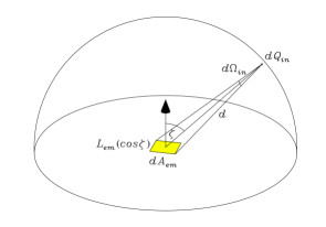
Figure 1: Sketch to illustrate the difference between emitted radiance $L_{\mathrm{em}}$, incident irradiance $dQ_{\mathrm{in}}$ and incident power $d\Phi_{\mathrm{in}}$.

name	variable in astrophysics	SI equivalent	SI unit
intensity, brightness	$I(\mathbfl{\hat{k}})$	$L(\mathbfl{\hat{k}})$	W m-2sr-1
energy density	$U=\frac{1}{c}\int_{4\pi}I(\mathbfl{\hat{k}})d\Omega$	$\frac{1}{c}Q$	Ws m-3
flux in direction $\mathbfl{\hat{a}}$	$F(\mathbfl{\hat{a}})=\int_{4\pi}I(\mathbfl{\hat{k}})\;\mathbfl{\hat{k}}^{\mathsf{T}}\mathbfl{\hat{a}}\;d\Omega$	$\frac{d\Phi}{dA}$	W m-2

Table 1: Table of commonly used radiometric quantities in astrophysics and their SI-compatible counterpart. All astrophysics quantities are often used in their spectral variant, i.e., per frequency or wave length interval. The direction $\mathbfl{\hat{a}}$ in the flux definition is the normal of the area element $d\mathbfl{A}$ in the SI definition of $\Phi$.

So far all quantities and their relations were local. Of interest is the situation were we have an emitting and an incident side. We illustrate the relations between either side by two examples. The quantities are marked by subscripts “em” and “in” depending on which site they relate to. Assume as in Fig. 1 that a surface $dA_{\mathrm{em}}$ is emitting into the entire half space $\Omega_{\mathrm{em}}=2\pi$. A small part of this flux is incident on an instrument at distance $d$ in direction $\mathbfl{\hat{k}}$ with aperture area $d\mathbfl{A}_{\mathrm{in}}$ pointing exactly in direction $-\mathbfl{\hat{k}}$. Then the power collected by the instrument is confined to the infinitesimal solid emission angle $d\Omega(\mathbfl{\hat{k}})=d\Omega_{\mathrm{em}}=dA_{\mathrm{in}}/d^{2}$. We have according to (2.7)

$$d\Phi_{\mathrm{em}} =L_{\mathrm{em}}(\mathbfl{\hat{k}})\,\cos\zeta\,dA_{\mathrm{em}}\;d\Omega_{\mathrm{em}}(\mathbfl{\hat{k}}) \text{flux emitted into}\;d\Omega_{\mathrm{em}}$$ (2.9)

$$=d\Phi_{\mathrm{in}} =L_{\mathrm{em}}(\mathbfl{\hat{k}})\,\cos\zeta\frac{dA_{\mathrm{em}}}{d^{2}}\,dA_{\mathrm{in}}=L_{\mathrm{em}}(\mathbfl{\hat{k}})\,d\Omega_{\mathrm{in}}dA_{\mathrm{in}} \text{flux collected from}\;d\Omega_{\mathrm{in}}$$ (2.10)

where $d\Omega_{\mathrm{in}}=\cos\zeta\,dA_{\mathrm{em}}/d^{2}$ is the solid angle subtended by the emitting surface at the observing instrument.

Figure 2: Sketch to illustrate $\cos^{4}\zeta$ dependence of $d\Phi_{\mathrm{in}}$ when $d\mathbfl{A}_{\mathrm{em}}$ and $d\mathbfl{A}_{\mathrm{in}}$ are parallel and their distance $z$ constant.

If instead we point the detector area $d\mathbfl{A}_{\mathrm{in}}$ vertically parallel to $-d\mathbfl{A}_{\mathrm{em}}$ (see Fig. 2), we have a reduced effective emission angle $d\Omega_{\mathrm{em}}=\mathbfl{\hat{k}}^{\mathsf{T}}d\mathbfl{A}_{\mathrm{in}}/d^{2}=\cos\zeta\,dA_{\mathrm{in}}/d^{2}$. If in addition we keep the vertical distance between emitter and receiver constant at a height $z$, their mutual distance becomes $d=z/\cos\zeta$. Altogether, the received power will in this setup be $d\Phi_{\mathrm{in}}=L_{\mathrm{em}}dA_{\mathrm{em}}dA_{\mathrm{in}}\cos^{2}\zeta/d^{2}=L_{\mathrm{em}}dA_{\mathrm{em}}dA_{\mathrm{in}}\cos^{4}\zeta/z^{2}$ instead of (2.10). The $\cos^{4}\zeta$ dependence represents the ideal vignetting for a pinhole camera. For large surfaces $dA_{\mathrm{em}}$ and imaging instruments, $d\Omega_{\mathrm{in}}$ is often constrained by the solid angle of the instrument resolution rather than by the size of $dA_{\mathrm{em}}$. In this case, $d\Omega_{\mathrm{in}}=A_{\mathrm{pixel}}/f^{2}$ depends on the focal length $f$ and the pixel area $A_{\mathrm{pixel}}$ of the instrument rather than on distance $d$ and the received power $d\Phi_{\mathrm{in}}$ per pixel does not change with distance form the emitting surface. From (2.10), the ratio

$$dQ_{\mathrm{in}}=\frac{d\Phi_{\mathrm{in}}}{dA_{\mathrm{in}}}=L_{\mathrm{em}}(\mathbfl{\hat{k}})\,\cos\zeta\;\frac{dA_{\mathrm{em}}}{d^{2}}=L_{\mathrm{em}}(\mathbfl{\hat{k}})d\Omega_{\mathrm{in}}\qquad[\mathrm{W/m^{2}}]$$ (2.11)

is the irradiance produced by photons from the small cone $d\Omega_{\mathrm{em}}=dA_{\mathrm{em}}/d^{2}$ around $\mathbfl{\hat{k}}$ at the site of the instrument. It is the relevant incident irradiance for a scattering particle at the location of the instrument in our example.

As a second example, consider the emitting surface replaced by a point source. Now, the emitting radiance $L_{\mathrm{em}}$ is not suitable any more to describe the source. However, we expect that we measure a radiant flux in direction $\mathbfl{\hat{k}}$ proportional to the solid angle $d\Omega_{\mathrm{em}}=dA_{\mathrm{in}}/d^{2}$ from photons which propagate inside this solid angle and hit the detector surface $dA_{\mathrm{in}}$ at distance $d$. Again we assume that the receiving aperture area $d\mathbfl{A}_{\mathrm{in}}$ points exactly to $-\mathbfl{\hat{k}}$ in direction to the source. We can therefore define a radiant intensity (2.8) of

$$I_{\mathrm{in}}(\mathbfl{\hat{k}})=\frac{d\Phi_{\mathrm{in}}}{d\Omega_{\mathrm{em}}}=\frac{d\Phi_{\mathrm{in}}}{dA_{\mathrm{in}}}\;d^{2}=Q_{\mathrm{in}}\;d^{2}\qquad[\mathrm{W/sr}]$$ (2.12)

which characterises the directional emission pattern of the point source. The radiant intensity is the relevant quantity to describe the far field of a scattering particle.

At first sight, there seems to be an inconsistency of units in (2.12) because irradiance $Q$ has units of [W/m²]. The problem can be traced back to the fact that $dA_{\mathrm{em}}/d^{2}$ was considered to be a solid angle. Since $dA_{\mathrm{em}}$ is an area, $d^{2}$ formally must have the units [m²/sr]. This unusual interpretation must be kept in mind when an area and the solid angle it subtends in some distant centre are compared.

The entire emitted power from the point source is

$$\Phi_{\mathrm{em}}=\Phi_{\mathrm{in}}=\int I_{\mathrm{in}}(\mathbfl{\hat{k}})d\Omega_{\mathrm{em}}(\mathbfl{\hat{k}})$$

An isotropic source with $I_{\mathrm{in}}=\mathrm{const}$ emits a power $\Phi_{\mathrm{em}}=4\pi I_{\mathrm{in}}$ and produces a local irradiance according to (2.12) of $Q_{\mathrm{in}}=\Phi_{\mathrm{em}}/4\pi d^{2}$.

3 Electrons at rest – classical Thomson scattering in the corona

In the following we will apply the above expressions to the scattering of Sun light at coronal electrons. The emitting area element will be extended to the visible solar surface, the receiving area element is replaced by the scattering electron. We will switch to a spherical coordinate system with its origin in the scattering site $\mathbfl{r}$ at distant $r$ from the solar centre and its zenith axis aligned with the radial direction from the Sun. Variable $d$ will continue to be the distance from the emitting surface element to the scattering site but because of the spherical symmetry, $\Phi_{\mathrm{in}}$ and $Q_{\mathrm{in}}$ will from now on depend on the distance $r$.

3.1 Irradiance of Sun light

The irradiance incident from the solar surface is obtained from (2.11) by extending $\Omega_{\mathrm{in}}=\Omega(r)$ over the part of the surface visible from distance $r$. In spherical coordinates $d\Omega=\sin\theta d\theta d\phi$ (for the geometry see Fig. 3), where $\theta$ and $\phi$ are the spherical zenith and azimuth angles.

$$Q_{\mathrm{in}}(r)=\int_{0}^{2\pi}\int_{0}^{\theta_{\mathrm{max}}}L(\cos\zeta)\;\sin\theta d\theta d\phi=2\pi\int_{0}^{\theta_{\mathrm{max}}}L(\cos\zeta)\;\sin\theta d\theta$$

$$=2\pi\int^{1}_{\cos\theta_{\mathrm{max}}}\mspace{-10.0mu}L(\cos\zeta)\;d\cos\theta\qquad[\mathrm{W/m^{2}}]$$ (3.1)

The ignorable azimuth angle $\phi$ could readily be integrated over because of the cylindrical symmetry about the zenith axis of the spherical coordinate system.

Figure 3: Sketch illustrating the geometry of the illumination of a point $S$ at finite distance $r$ (left) from the Sun’s centre and at infinite distance (right).

In (3.1), $\zeta$ is the zenith angle of the radiance beam direction with the surface normal. We have to find its relation with the integration variable $\theta$. By the law of sines we have at a distance $r$ and for a solar radius $R_{\odot}$ (see Fig. 3, note $\sin\zeta=\sin(\pi-\zeta$))

$$\frac{\sin\zeta}{r}=\frac{\sin\theta}{R_{\odot}},\qquad\frac{1}{r}=\frac{\sin\theta_{\mathrm{max}}}{R_{\odot}}$$ (3.2)

$$\text{so that}\quad\cos\zeta=\sqrt{1-(\frac{r}{R_{\odot}})^{2}\sin^{2}\theta}=\sqrt{1-(\frac{r}{R_{\odot}})^{2}+(\frac{r}{R_{\odot}})^{2}\cos^{2}\theta}$$ (3.3)

where the second equation in (3.2) refers to the view from the observer onto the solar limb with maximum $\theta$ such that $\zeta=\pi/2$. Equation (3.3) is used in the following to express the argument $\cos\zeta$ in terms of the integration variable $\cos\theta$.

For the Sun, the surface radiance is approximately given by [e.g., Neckel and Labs, 1994, Neckel, 1996]

$$L(\cos\zeta)=L_{\odot}(1-u+u\cos\zeta)$$ (3.4)

with $L_{\odot}$ the radiance in vertical direction. The limb darkening parameter $u$ has been empirically determined to about 0.6 in the optical wavelength range. If we insert (3.4) into (3.1) we find

$$Q_{\mathrm{in}}(r)=L_{\odot}[(1-u)I_{0}(r)+uI_{1}(r)]$$ (3.5)

which contains the two integrals

$$I_{0}(r)=2\pi\int_{\cos\theta_{\mathrm{max}}(r)}^{1}\mspace{-15.0mu}d\cos\theta,\quad I_{1}(r)=2\pi\int_{\cos\theta_{\mathrm{max}}(r)}^{1}\mspace{-15.0mu}\cos\zeta\,d\cos\theta$$ (3.6)

The integrals are calculated in the appendix A after expressing $\cos\zeta$ in terms of $\cos\theta$ by means of (3.3). Inserting the analytical expressions (A.3) and (A.5) for the integrals in (3.5) gives

$$Q_{\mathrm{in}}(r)=2\pi L_{\odot}[(1-u)(1-\cos\theta_{\mathrm{max}})+\frac{u}{2}\;\left[1-\frac{\cos^{2}\theta_{\mathrm{max}}}{\sin\theta_{\mathrm{max}}}\ln(\frac{1+\sin\theta_{\mathrm{max}}}{\cos\theta_{\mathrm{max}}})\right]]$$

$$=2\pi L_{\odot}[(1-\frac{u}{2})(1-\cos\theta_{\mathrm{max}})+\frac{u}{2}\cos\theta_{\mathrm{max}}\;\left[1-\frac{\cos\theta_{\mathrm{max}}}{\sin\theta_{\mathrm{max}}}\ln(\frac{1+\sin\theta_{\mathrm{max}}}{\cos\theta_{\mathrm{max}}})\right]]$$ (3.7)

For $r\rightarrow\infty$ we have $\theta_{\mathrm{max}}\rightarrow R_{\odot}/r$ and (see appendix A)

$$Q_{\mathrm{in}}(r)\xrightarrow{r\rightarrow\infty}L_{\odot}[(1-u)I^{\infty}_{0}+uI^{\infty}_{1}]$$

$$\simeq\pi L_{\odot}[(1-u)\theta^{2}_{\mathrm{max}}+u{\textstyle\frac{2}{3}}\theta^{2}_{\mathrm{max}}]=\pi L_{\odot}(1-\frac{u}{3})\theta^{2}_{\mathrm{max}}=\frac{\pi R_{\odot}^{2}}{r^{2}}\bar{L}_{\odot}$$

where $\bar{L}_{\odot}=L_{\odot}(1-u/3)$ is the average radiance of the solar disk. This is consistent with the integration of the original expression in (3.1) in the far-distance limit $r\rightarrow\infty$ such that $\sin\theta\simeq\theta\simeq\rho/r$ and $\cos\zeta=\sqrt{1-\sin^{2}\zeta}\simeq\sqrt{1-(\rho/R_{\odot})^{2}}$ (see Fig. 3)

$$Q_{\mathrm{in}}(r)\xrightarrow{r\rightarrow\infty}\frac{2\pi}{r^{2}}\int_{0}^{R_{\odot}}L(\sqrt{1-(\frac{\rho}{R_{\odot}})^{2}})\;\rho d\rho$$

$$=\pi(\frac{R_{\odot}}{r})^{2}\int_{0}^{1}L(\sqrt{1-(\frac{\rho}{R_{\odot}})^{2}})\;d(\frac{\rho}{R_{\odot}})^{2}\qquad\text{substitute}\;1-(\frac{\rho}{R_{\odot}})^{2}=\cos^{2}\zeta=x$$

$$=\pi(\frac{R_{\odot}}{r})^{2}L_{\odot}\int_{0}^{1}[1-u+ux^{1/2}]dx=\pi(\frac{R_{\odot}}{r})^{2}L_{\odot}[\left.(1-u)x\right|_{0}^{1}+\frac{2}{3}u\left.x^{3/2}\right|_{0}^{1}]$$

$$=\pi(\frac{R_{\odot}}{r})^{2}L_{\odot}[(1-u)+\frac{2}{3}u]=\pi(\frac{R_{\odot}}{r})^{2}\bar{L}_{\odot}$$ (3.8)

The power radiated from the entire solar surface (luminosity) is

$$\Phi_{\odot}=4\pi r^{2}\;Q_{\mathrm{in}}(r)=4\pi^{2}R_{\odot}^{2}\bar{L}_{\odot}=\pi\bar{L}_{\odot}\times\text{solar surface}\qquad[\mathrm{W}]$$

3.2 Anisotropy of solar irradiance

In the previous chapter we have only calculated the scalar irradiance of Sun light at a given distance from Sun. For treating the scattering adequately we also need to know how the electric field fluctuations of the light from the solar surface are oriented. In order to assess this property, we have to extend the scalar radiance and irradiance to space tensors. The concept is well known in optics to characterise the correlation and polarisation of electromagnetic wave fields [see e.g., Wolf, 2007]. Most often this concept is applied to beams of light propagating in a well defined direction for which the field correlation can be described by a 2$\times$2 coherency matrix spanning the plane normal to the beam propagation direction. Since we consider here a spatially extended source with light from different directions, a 3$\times$3 matrix is required instead. We first extend the definition of the power spectral density (2.2) in an obvious way

$$\lim_{V\rightarrow\infty}\frac{1}{V}<\!\mathbfl{\tilde{E}}_{V}(\mathbfl{k})\mathbfl{\tilde{E}}_{V}^{*\mathsf{T}}(\mathbfl{k})\!>\;=\int\!\mathbfl{R}(\Delta\mathbfl{r})\;e^{-i\mathbfl{k}^{\mathsf{T}}\Delta\mathbfl{r}}\;d^{3}\Delta\mathbfl{r}$$ (3.9)

$$\mathbfl{R}(\Delta\mathbfl{r})=\;<\!\mathbfl{E}(\mathbfl{r},t)\mathbfl{E}^{\mathsf{T}}(\mathbfl{r}+\Delta\mathbfl{r},t)\!>$$

where the correlation matrix $\mathbfl{R}$ is symmetric and has a trace of $R$ as defined in (2.2). The according radiance matrix is in analogy to (2.4)

$$\mathbfl{L}(\mathbfl{\hat{k}})=c\epsilon_{0}\lim_{V\rightarrow\infty}\frac{1}{V}\int\!<\!\mathbfl{\tilde{E}}_{V}(k\mathbfl{\hat{k}})\mathbfl{\tilde{E}}_{V}^{*\mathsf{T}}(k\mathbfl{\hat{k}})\!>k^{2}\,dk$$

Since the radiance selects only those wave field components from the spectrum which propagate along $\mathbfl{\hat{k}}$, we have $\mathbfl{L}(\mathbfl{\hat{k}})\mathbfl{\hat{k}}=0$. Hence $\mathbfl{L}(\mathbfl{\hat{k}})$ spans only the subspace perpendicular to $\mathbfl{\hat{k}}$ and could be reduced to a 2$\times$2 submatrix which has the same properties as a conventional coherency matrix (see appendix C.2). Finally, we need the same generalisation for the irradiance from (2.5) and (2.6)

$$\mathbfl{Q}=\int_{4\pi}\mathbfl{L}(\mathbfl{\hat{k}})d\Omega(\mathbfl{\hat{k}})=c\epsilon_{0}\lim_{V\rightarrow\infty}\frac{1}{V}\int\!<\!\mathbfl{\tilde{E}}_{V}(\mathbfl{k})\mathbfl{\tilde{E}}_{V}^{*\mathsf{T}}(\mathbfl{k})\!>\,d^{3}\mathbfl{k}$$ (3.10)

$$=c\epsilon_{0}\mathbfl{R}(0)=c\epsilon_{0}<\!\mathbfl{E}(\mathbfl{r},t)\mathbfl{E}^{\mathsf{T}}(\mathbfl{r},t)\!>$$

All these tensorialised quantities reduce to their scalar analogues used in the previous chapter by forming the trace.

In principle, we now have to repeat the integration (3.1) as in the previous chapter, however for each matrix element separately. For our problem the radiance $\mathbfl{L}(\mathbfl{\hat{k}})$ in (3.10) is non-zero only for a limited cone $\Omega(r)$ of directions $\mathbfl{\hat{k}}$ from the visible solar surface to the scattering site $\mathbfl{r}$. Therefore the integration is effectively over $\Omega(r)$ rather than over $4\pi$ as in the general case in (3.10). The integration is also greatly simplified by the assumption that the radiance from the solar surface is unpolarised [Kemp et al., 1987]. The radiance matrix is then (see appendix C.2)

$$\mathbfl{L}(\mathbfl{\hat{k}})=\frac{1}{2}L(\cos\zeta)\,(\mathbfl{\hat{e}}_{1}\mathbfl{\hat{e}}_{1}^{\mathsf{T}}+\mathbfl{\hat{e}}_{2}\mathbfl{\hat{e}}^{\mathsf{T}}_{2})=\frac{1}{2}L(\cos\zeta)\,(\boldsymbol{1}-\mathbfl{\hat{k}}\mathbfl{\hat{k}}^{\mathsf{T}})$$ (3.11)

where $L(\cos\zeta)$ is the scalar radiance (3.4), $\mathbfl{\hat{e}}_{1}$ and $\mathbfl{\hat{e}}_{2}$ are two mutually orthogonal polarisation vectors spanning the plane perpendicular to $\mathbfl{\hat{k}}$ and $\boldsymbol{1}$ is the identity matrix. In case that $\mathbfl{L}$ is polarised all matrix elements $\mathbfl{\hat{e}}_{i}\mathbfl{\hat{e}}^{\mathsf{T}}_{j}$ are needed and weighted with different coefficients related to the Stokes parameters. We then cannot use the second form in (3.11). But for the unpolarised incident radiation assumed here, the second form is favourable because $\mathbfl{\hat{e}}_{1}$ and $\mathbfl{\hat{e}}_{2}$ do not need to be specified. The final expression for the irradiance matrix at the scattering site is then from (3.10) and (3.11)

$$\mathbfl{Q}_{\mathrm{in}}(\mathbfl{r})=\frac{1}{2}\int_{\Omega}L(\cos\zeta)\,(\boldsymbol{1}-\mathbfl{\hat{k}}\mathbfl{\hat{k}}^{\mathsf{T}})d\Omega(\mathbfl{\hat{k}})$$ (3.12)

where instead of $4\pi$ we only integrate the directions $\mathbfl{\hat{k}}$ over the solar surface $\Omega(r)$ visible from distance $r$.

In the coordinate system of Fig. 4 we can write explicitly the propagation direction $\mathbfl{\hat{k}}$ of a given beam from a point on the solar surface to the scattering site (points E and S in Fig. 4) as

$$\mathbfl{\hat{k}}=\left(\begin{array}[]{c}\!\!\cos\phi\sin\theta\!\!\\ \!\!\sin\phi\sin\theta\!\!\\ \!\!\cos\theta\!\!\end{array}\right)$$ (3.13)

We can now express the radiance matrix elements in the integrand of (3.12) for different locations on the solar surface. From (3.11) and (3.13) we find

$$\mathbfl{\hat{x}}\mathbfl{L}(\mathbfl{\hat{k}})\mathbfl{\hat{x}} =\frac{1}{2}L(\cos\zeta)\,(1-\cos^{2}\phi\sin^{2}\theta)$$

$$\mathbfl{\hat{y}}\mathbfl{L}(\mathbfl{\hat{k}})\mathbfl{\hat{y}} =\frac{1}{2}L(\cos\zeta)\,(1-\sin^{2}\phi\sin^{2}\theta)$$

$$\mathbfl{\hat{z}}\mathbfl{L}(\mathbfl{\hat{k}})\mathbfl{\hat{z}} =\frac{1}{2}L(\cos\zeta)\,(1-\cos^{2}\theta)$$

$$\mathbfl{\hat{x}}\mathbfl{L}(\mathbfl{\hat{k}})\mathbfl{\hat{y}}=\mathbfl{\hat{y}}\mathbfl{L}(\mathbfl{\hat{k}})\mathbfl{\hat{x}} =\frac{1}{2}L(\cos\zeta)\,\cos\phi\sin\phi\sin^{2}\theta)$$

$$\mathbfl{\hat{x}}\mathbfl{L}(\mathbfl{\hat{k}})\mathbfl{\hat{z}}=\mathbfl{\hat{z}}\mathbfl{L}(\mathbfl{\hat{k}})\mathbfl{\hat{x}} =-\frac{1}{2}L(\cos\zeta)\,\cos\phi\sin\theta\cos\theta$$

$$\mathbfl{\hat{y}}\mathbfl{L}(\mathbfl{\hat{k}})\mathbfl{\hat{z}}=\mathbfl{\hat{z}}\mathbfl{L}(\mathbfl{\hat{k}})\mathbfl{\hat{y}} =-\frac{1}{2}L(\cos\zeta)\,\sin\phi\sin\theta\cos\theta$$

Note that the off-diagonal elements are all odd in $\phi$ and will therefore vanish in the subsequent integration over the visible solar surface. Note also that $\mathbfl{\hat{x}}\mathbfl{\hat{x}}^{\mathsf{T}}+\mathbfl{\hat{y}}\mathbfl{\hat{y}}^{\mathsf{T}}+\mathbfl{\hat{z}}\mathbfl{\hat{z}}^{\mathsf{T}}$ is the unit matrix and $\mathrm{trace}({\mathbfl{L}})$ reproduces the scalar $L(\cos\zeta)$ which was integrated in the previous chapter.

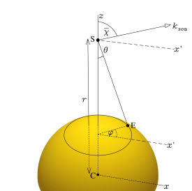
Figure 4: Sketch illustrating the geometry of scattering at point S. The centre of the coordinate system is the solar centre C, the radiation originates from a point E on the solar surface at distance $r$ along the $z$ axis. The scattered ray $\mathbfl{k}_{\mathrm{sc}}$ lies in the $\mathbfl{\hat{x}},\mathbfl{\hat{z}}$ plane which defines the $x$-axis. The dashed axes $x^{\prime}$ are drawn to help the eye and are all parallel to the $x$ axis. The $y$-axis is normal to $\mathbfl{\hat{x}}$ and $\mathbfl{\hat{z}}$.

The contributions of the emission from all points like E in Fig. 4 to the irradiance at point S at distance $r$ can now be summed up. Only elements which are even in $\phi$ survive the integration in azimuth angle so that we readily obtain after the $\phi$ integration using (3.12) and (3.13)

$$\mathbfl{Q}_{\mathrm{in}}(\mathbfl{r})=\frac{1}{2}\int_{\Omega}L(\cos\zeta)\,(\boldsymbol{1}-\mathbfl{\hat{k}}\mathbfl{\hat{k}}^{\mathsf{T}})\,\sin\theta d\theta d\phi$$ (3.14)

$$=\frac{2\pi}{2}\int_{0}^{\theta\mathrm{max}}L(\cos\zeta)\begin{pmatrix}{\textstyle\!\frac{1}{2}}+{\textstyle\!\frac{1}{2}}\cos^{2}\theta&0&0\\ 0&{\textstyle\!\frac{1}{2}}+{\textstyle\!\frac{1}{2}}\cos^{2}\theta&0\\ 0&0&1-\cos^{2}\theta\end{pmatrix}d\cos\theta$$ (3.15)

where $\sin^{2}\theta$ was replaced by $1-\cos^{2}\theta$ throughout. If we insert the limb-darkened solar radiance (3.4) into (3.15) we get

$$\mathbfl{Q}_{\mathrm{in}}(\mathbfl{r})=\frac{L_{\odot}}{2}[(1-u)\begin{pmatrix}\frac{I_{0}+J_{0}}{2}&0&0\\ 0&\frac{I_{0}+J_{0}}{2}&0\\ 0&0&I_{0}-J_{0}\end{pmatrix}+u\begin{pmatrix}\frac{I_{1}+J_{1}}{2}&0&0\\ 0&\frac{I_{1}+J_{1}}{2}&0\\ 0&0&I_{1}-J_{1}\end{pmatrix}]$$

where we introduced two new integrals $I_{1}$ and $J_{1}$. The integrals of the $\theta$-independent terms in the matrix elements in eq. 3.15) agree with the known integrals $I_{0}$, $I_{1}$. The contributions of the $\cos^{2}\theta$ terms in the matrix elements lead to two new integrals

$$J_{0}(r)=2\pi\int_{\cos\theta_{\mathrm{max}}(r)}^{1}\mspace{-15.0mu}\cos^{2}\theta\,d\cos\theta,\quad J_{1}(r)=2\pi\int_{\cos\theta_{\mathrm{max}}(r)}^{1}\mspace{-15.0mu}\cos\zeta\cos^{2}\theta\,d\cos\theta$$ (3.16)

The integrals are calculated in the appendix A again after expressing $\cos\zeta$ in terms of $\cos\theta$ as in (3.3). If instead of (3.4) we wanted to use limb-darkening laws with higher powers in $\cos\zeta$ we obtain corresponding integrals $I_{n}$ and $J_{n}$ for which we also derive analytic expressions in appendix A. Finally we can write the non-zero elements of the local irradiance matrix as

$$Q_{\mathrm{in},xx}(r)=Q_{\mathrm{in},yy}(r)= \;{\textstyle\!\frac{1}{4}}L_{\odot}((1-u)(I_{0}+J_{0})+u(I_{1}+J_{1}))$$

$$Q_{\mathrm{in},zz}(r)= \;{\textstyle\!\frac{1}{2}}L_{\odot}((1-u)(I_{0}-J_{0})+u(I_{1}-J_{1}))$$

A combination of the integrals introduced by [Minnaert, 1930] and often preferred in the literature is

$$C=\frac{I_{0}+J_{0}}{2\pi},\qquad D=\frac{I_{1}+J_{1}}{2\pi}$$

$$A=\frac{3J_{0}-I_{0}}{2\pi},\qquad B=\frac{3J_{1}-I_{1}}{2\pi}$$

$$Q_{\mathrm{in},xx}=Q_{\mathrm{in},yy}=\frac{\pi L_{\odot}}{2}((1-u)C+uD)$$ (3.17)

$$Q_{\mathrm{in},xx}-Q_{\mathrm{in},zz}={\textstyle\!\frac{1}{4}}L_{\odot}((1-u)[(I_{0}+J_{0})-2(I_{0}-J_{0})]$$

$$\hskip 80.00012pt+u[(I_{1}+J_{1})-2(I_{1}-J_{1})])$$

$$=\frac{L_{\odot}}{4}((1-u)(3J_{0}-I_{0})+u(3J_{1}-I_{1}))$$

$$=\frac{\pi L_{\odot}}{2}((1-u)A+uB)$$ (3.18)

$$\text{or}\quad\mathbfl{Q}_{\mathrm{in}}(\mathbfl{r})=\frac{\pi L_{\odot}}{2}\big{[}((1-u)C+uD)\boldsymbol{1}-((1-u)A+uB)\mathbfl{\hat{r}}\mathbfl{\hat{r}}^{\mathsf{T}}\big{]}$$ (3.19)

where in the last row we replaced $\mathbfl{\hat{z}}$ of the local coordinate system (see Fig. 4) by the more general unit vector $\mathbfl{\hat{r}}$ from the solar centre to the point for which the irradiance is calculated. The coefficients $A$, $B$, $C$ and $D$ depend only on the distance $r$ from the solar centre. Some useful properties of these coefficients are derived in appendix A.

To this end we are able to characterise the field fluctuations at a distance $r$ (point S in Fig. 4) from the solar centre. It is not surprising that due to symmetry their polarisations in $x$ and $y$ are identical. As also expected for $r\rightarrow\infty$,

$$Q_{\mathrm{in},xx}=Q_{\mathrm{in},yy}\rightarrow\frac{\pi L_{\odot}}{2}((1-u)-\frac{2}{3}u)(\frac{R_{\odot}}{r})^{2}=\frac{\pi}{2}(\frac{R_{\odot}}{r})^{2}\bar{L}_{\odot}$$ (3.20)

$$Q_{\mathrm{in},zz}=\frac{\pi L_{\odot}}{2}((1-u)(C-A)-u(D-B))\rightarrow r^{-4}$$ (3.21)

i.e., the radial element decreases much faster then the tangential elements. Each of the latter approach half the total asymptotic irradiance (3.8).

3.3 Scattering of solar irradiance

We start again with scalar variables to discuss the scattering process in general. The principle will then be extended to the matrix quantities derived in the previous chapter. We assume as in (2.11) that the irradiance $dQ_{\mathrm{in}}=L(\mathbfl{\hat{k}}_{\mathrm{in}})d\Omega_{\mathrm{in}}$ describes the field fluctuations of a narrow beam in direction $\mathbfl{\hat{k}}_{\mathrm{in}}$ incident at the scattering site $\mathbfl{r}$. If the total scattering cross section from a single scatterer is $\sigma$, the total number of scattered photons is equivalent to the totally scattered power (the hat on $\hat{\Phi}$ indicates normalisation to a single scattering centre)

$$d\hat{\Phi}=\sigma dQ_{\mathrm{in}}=\sigma L(\mathbfl{\hat{k}}_{\mathrm{in}})d\Omega_{\mathrm{in}}\qquad[\mathrm{W}]$$ (3.22)

The single scattering centre is the source of a scattered radiant intensity which describes the angular distribution of the scattered photons. If we only count the number of scattered photons in a special direction $\mathbfl{\hat{k}}_{\mathrm{sc}}$, we have to replace the total scattering cross section $\sigma=\int(d\sigma/d\Omega_{\mathrm{sc}})\;d\Omega_{\mathrm{sc}}$ by the differential cross section $d\sigma/d\Omega_{\mathrm{sc}}$. This yields a scattered radiant intensity in the scattering direction $\mathbfl{\hat{k}}_{\mathrm{sc}}$ of

$$dI(\mathbfl{r},\mathbfl{\hat{k}}_{\mathrm{sc}})=\frac{d\Phi_{\mathrm{sc}}}{d\Omega_{\mathrm{sc}}}=\frac{d\sigma}{d\Omega_{\mathrm{sc}}}(\mathbfl{\hat{k}}_{\mathrm{in}},\mathbfl{\hat{k}}_{\mathrm{sc}})dQ_{\mathrm{in}}(\mathbfl{r})=\frac{d\sigma}{d\Omega_{\mathrm{sc}}}(\mathbfl{\hat{k}}_{\mathrm{in}},\mathbfl{\hat{k}}_{\mathrm{sc}})L(\mathbfl{\hat{k}}_{\mathrm{in}})d\Omega_{\mathrm{in}}\qquad[\mathrm{W/sr}]$$ (3.23)

Integrating over all scattering directions yields again the total scattered power (3.22). We collect the scattered photons at $\mathbfl{r}_{\mathrm{obs}}=\mathbfl{r}+\ell\mathbfl{\hat{k}}_{\mathrm{sc}}$ in an aperture area $\mathbfl{A}_{\mathrm{aperture}}$ with normal in $-\mathbfl{\hat{k}}_{\mathrm{sc}}$. The aperture then subtends a solid angle $d\Omega_{\mathrm{sc}}=A_{\mathrm{aperture}}/\ell^{2}$ at the scattering site and the instrument integrates over all scattering directions $\mathbfl{\hat{k}}_{\mathrm{sc}}$ inside this solid angle. Hence from the single scattering centre we obtain a radiant flux in the instrument at distance $\ell$ equivalent to the power

$$d\hat{\Phi}(\mathbfl{r}_{\mathrm{obs}})=d\Omega_{\mathrm{sc}}\,dI(\mathbfl{r},\mathbfl{\hat{k}}_{\mathrm{sc}})=\frac{A_{\mathrm{aperture}}}{\ell^{2}}\,dI(\mathbfl{r},\mathbfl{\hat{k}}_{\mathrm{sc}})\qquad[\mathrm{W}]$$ (3.24)

which corresponds to an irradiance at the instrument of

$$dQ_{\mathrm{sc}}(\mathbfl{r}_{\mathrm{obs}})=\frac{d\hat{\Phi}(\mathbfl{r}_{\mathrm{obs}})}{A_{\mathrm{aperture}}}=\frac{dI(\mathbfl{r},\mathbfl{\hat{k}}_{\mathrm{sc}})}{\ell^{2}}\,=\frac{d\sigma}{\ell^{2}d\Omega_{\mathrm{sc}}}(\mathbfl{\hat{k}}_{\mathrm{in}},\mathbfl{\hat{k}}_{\mathrm{sc}})\;L(\mathbfl{\hat{k}}_{\mathrm{in}})d\Omega_{\mathrm{in}}$$

$$=\frac{d\sigma}{\ell^{2}d\Omega_{\mathrm{sc}}}(\mathbfl{\hat{k}}_{\mathrm{in}},\mathbfl{\hat{k}}_{\mathrm{sc}})\;dQ_{\mathrm{in}}\qquad[\mathrm{W/m^{2}}]$$ (3.25)

Note the difference between $d\sigma/d\Omega_{\mathrm{sc}}$ in (3.23) and $d\sigma/\ell^{2}d\Omega_{\mathrm{sc}}$ in (3.25). While the former has the units [m²/sr] the latter is the dimensionless ratio of two areas, namely the influx area $d\sigma$ from which incident photons are redirected into the solid angle $d\Omega_{\mathrm{sc}}$ around the scattering direction $\mathbfl{\hat{k}}_{\mathrm{sc}}$ which is subtended by the detection area $\ell^{2}d\Omega_{\mathrm{sc}}$ at distance $\ell$. Since the number of photons is preserved, this area ratio is just the ratio of scattered and incident irradiances. The problem here is the same as with $d^{2}$ in (2.12). Formally we require that $\ell^{2}$ in (3.25) has the units [m²/sr] so that $\ell^{2}d\Omega_{\mathrm{sc}}$ represents an area in [m²].

A distribution of many scattering centres results in an extended radiating volume. We call $N_{e}$ the local number density of the scattering centres. Then the number of scatterers which is visible in the instrument is $N_{e}(\mathbfl{r})\ell^{2}d\Omega_{\mathrm{obs}}d\ell$ where $d\ell$ is the depth of the scattering volume at $\mathbfl{r}$ along the line-of-sight direction $\mathbfl{\hat{k}}_{\mathrm{sc}}$. The solid angle $d\Omega_{\mathrm{obs}}$ is the smaller of either the angle which the scattering cloud subtends at the instrument or the angle of the instrument’s pixel field of view. Hence, $d\Omega_{\mathrm{obs}}$ plays the same role with respect to the projected area of the scattering volume as $d\Omega_{\mathrm{in}}$ with respect to the solar surface element $dA_{\mathrm{em}}$. For an imaging coronagraph which well resolves the cloud of scattering centres, the solid angle of the volume visible to a pixel is often limited by the pixel resolution of the instrument rather than the size of the cloud. In this case $d\Omega_{\mathrm{obs}}=A_{\mathrm{pixel}}/f^{2}$ where $A_{\mathrm{pixel}}$ is the physical pixel area and $f$ the instrument focal length. Instead of (3.24), the photon flux per pixel for an observer at $\mathbfl{r}_{\mathrm{obs}}=\mathbfl{r}+\ell\mathbfl{\hat{k}}_{\mathrm{sc}}$ in the case of volume scattering is

$$d\Phi(\mathbfl{r}_{\mathrm{obs}})=N_{e}(\mathbfl{r})\ell^{2}d\Omega_{\mathrm{obs}}\,d\ell\;d\hat{\Phi}_{\mathrm{sc}}(\mathbfl{r}_{\mathrm{obs}})=N_{e}(\mathbfl{r})\ell^{2}d\Omega_{\mathrm{obs}}\,d\ell\;d\Omega_{\mathrm{sc}}\,dI(\mathbfl{r},\mathbfl{\hat{k}}_{\mathrm{sc}})$$

$$=\frac{A_{\mathrm{pixel}}A_{\mathrm{aperture}}}{f^{2}}N_{e}(\mathbfl{r})\;d\ell\;dI(\mathbfl{r},\mathbfl{\hat{k}}_{\mathrm{sc}})\qquad[\mathrm{W}]$$ (3.26)

Different from the $d\hat{\Phi}$ in the single scattering case (3.24), $d\Phi_{\mathrm{sc}}$ in (3.26) has no more explicit dependence on distance $\ell$ (there is still an implicit dependence through $N_{e}(\mathbfl{r})$, $d\sigma/d\Omega_{\mathrm{sc}}$ and $dI(\mathbfl{r},\mathbfl{\hat{k}}_{\mathrm{sc}})$, though). The units of $\ell^{2}$ [m²/sr] in (3.25) are now adopted by $f^{2}$ since $f^{2}d\Omega_{\mathrm{obs}}$ is the pixel area in [m²].

We have not specified the nature of the scattering yet. Thomson scattering is one of the simplest possible scattering mechanisms. This is why Rayleigh (1871) could derive it with few basic assumptions (the particle is at rest, unbound and much smaller than $2\pi/k$) and without making any further guess about the nature of the particle. As we have seen, the solar irradiance at the scattering site at $\mathbfl{r}$ is anisotropic, i.e., it has different field strengths in tangential and radial direction. Thomson scattering of these fluctuations modifies this incident polarisation further. The scattering is due to the dipole excitation of free electrons such that the radiating dipole axis is directed along the incident electric field $\mathbfl{E}_{\mathrm{in}}$. Provided the driving field strength $E_{\mathrm{in}}$ is well below $m_{e}c^{2}k/e$ so that the electron is not oscillating with a relativistic velocity, the orientation of the scattered field is just the projection of the incident field $\mathbfl{E}_{\mathrm{in}}$ into the transverse polarisation modes of the scattered wave which propagates in direction $\mathbfl{\hat{k}}_{\mathrm{sc}}$. The scattered electric field at some distance $\ell$ from the scattering electron at $\mathbfl{r}$ is therefore [Jackson, 1998]

$$\mathbfl{E}_{\mathrm{sc}}(\mathbfl{r}+\ell\mathbfl{\hat{k}}_{\mathrm{sc}},t)=-\frac{r_{e}}{\ell}\mathcal{P}_{\mathbfl{\hat{k}}_{\mathrm{sc}}}\mathbfl{E}_{\mathrm{in}}(\mathbfl{r},t-\frac{\ell}{c})$$ (3.27)

where $r_{e}$ is the classical electron radius

$$r_{e}=\frac{e^{2}}{4\pi\epsilon_{0}m_{e}c^{2}}=2.8179\>10^{-15}\mathrm{m}$$

at which the Coulomb potential energy equals the electron rest mass energy $m_{e}c^{2}$. The minus sign in (3.27) accounts for the phase shift of $\pi$ between the electron oscillation and the driving field, the time retardation $\ell/c$ for the phase delay of the scattered field after travelling the distance $\ell$. Both will be irrelevant for the stationary irradiances calculated here. Finally, $\mathcal{P}_{\mathbfl{\hat{k}}_{\mathrm{sc}}}$ is a projection normal to the propagation direction $\mathbfl{\hat{k}}_{\mathrm{sc}}$ [Hutchinson, 2002], defined as

$$\mathcal{P}_{\mathbfl{\hat{k}}_{\mathrm{sc}}}=(\boldsymbol{1}-\mathbfl{\hat{k}}_{\mathrm{sc}}\mathbfl{\hat{k}}^{\mathsf{T}}_{\mathrm{sc}})\quad\text{which satisfies}$$

$$\mathcal{P}^{\mathsf{T}}_{\mathbfl{\hat{k}}_{\mathrm{sc}}}=\mathcal{P}_{\mathbfl{\hat{k}}_{\mathrm{sc}}},\qquad\mathcal{P}^{2}_{\mathbfl{\hat{k}}_{\mathrm{sc}}}=\mathcal{P}_{\mathbfl{\hat{k}}_{\mathrm{sc}}},\qquad\mathcal{P}_{\mathbfl{\hat{k}}_{\mathrm{sc}}}\mathbfl{\hat{k}}_{\mathrm{sc}}=0,\quad\text{and}\quad\mathcal{P}_{\mathbfl{\hat{k}}_{\mathrm{sc}}}\mathbfl{\hat{p}}=\mathbfl{\hat{p}}$$ (3.28)

for every polarisation direction $\mathbfl{\hat{p}}$ of the scattered radiation since it is normal to $\mathbfl{\hat{k}}_{\mathrm{sc}}$.

The basic Thomson scattering law (3.27) can easily be extended to describe the scattering effect on the irradiance matrix,

$$\mathbfl{Q}_{\mathrm{sc}}(\mathbfl{r}+\ell\mathbfl{\hat{k}}_{\mathrm{sc}})=c\epsilon_{0}<\!\mathbfl{E}_{\mathrm{sc}}(\mathbfl{r}+\ell\mathbfl{\hat{k}}_{\mathrm{sc}},t)\mathbfl{E}^{*\mathsf{T}}_{\mathrm{sc}}(\mathbfl{r}+\ell\mathbfl{\hat{k}}_{\mathrm{sc}},t)\!>$$

$$=c\epsilon_{0}\frac{r_{e}^{2}}{\ell^{2}}<\!\mathcal{P}_{\mathbfl{\hat{k}}_{\mathrm{sc}}}\mathbfl{E}_{\mathrm{in}}(\mathbfl{r},t-\frac{\ell}{c})(\mathcal{P}_{\mathbfl{\hat{k}}_{\mathrm{sc}}}\mathbfl{E}_{\mathrm{in}})^{\mathsf{T}}(\mathbfl{r},t-\frac{\ell}{c})\!>$$

$$=c\epsilon_{0}\frac{r_{e}^{2}}{\ell^{2}}\mathcal{P}_{\mathbfl{\hat{k}}_{\mathrm{sc}}}\!\!<\!\mathbfl{E}_{\mathrm{in}}\mathbfl{E}^{\mathsf{T}}_{\mathrm{in}}\!>\!(\mathbfl{r})\,\mathcal{P}_{\mathbfl{\hat{k}}_{\mathrm{sc}}}=\frac{r_{e}^{2}}{\ell^{2}}\mathcal{P}_{\mathbfl{\hat{k}}_{\mathrm{sc}}}\mathbfl{Q}_{\mathrm{in}}(\mathbfl{r})\,\mathcal{P}_{\mathbfl{\hat{k}}_{\mathrm{sc}}}$$ (3.29)

Obviously, for sufficiently large distance $\ell$ from the scattering source the scattered waves which contribute to $\mathbfl{Q}_{\mathrm{sc}}$ all propagate in direction $\mathbfl{\hat{k}}_{\mathrm{sc}}$. Therefore $\mathbfl{Q}_{\mathrm{sc}}\mathbfl{\hat{k}}_{\mathrm{sc}}=0$ and the 2$\times$2 submatrix spanning the space perpendicular to $\mathbfl{\hat{k}}_{\mathrm{sc}}$ characterises the polarisation state of the scattered beam. Note that the reverse reasoning is not generally true. Contrary to $\mathbfl{L}$, the irradiance $\mathbfl{Q}$ may be superposed of wave fields from different directions and $\mathbfl{Q}\mathbfl{\hat{k}}=0$ does not necessarily imply that these waves all propagate along $\mathbfl{\hat{k}}$. To estimate polarisation properties from a general 3$\times$3 correlation matrix has been an issue for a long time [see, e.g. Ellis et al., 2005]. In the scattering case and at a position $\mathbfl{r}_{\mathrm{obs}}=\mathbfl{r}+\ell\mathbfl{\hat{k}}_{\mathrm{sc}}$ in the far field of the scatterer, the irradiance component polarised along $\mathbfl{\hat{p}}\perp\mathbfl{\hat{k}}_{\mathrm{sc}}$ is therefore simply obtained from the matrix element

$$\mathbfl{\hat{p}}^{\mathsf{T}}\mathbfl{Q}_{\mathrm{sc}}(\mathbfl{r}_{\mathrm{obs}})\mathbfl{\hat{p}}=\frac{r_{e}^{2}}{\ell^{2}}\mathbfl{\hat{p}}^{\mathsf{T}}\mathcal{P}_{\mathbfl{\hat{k}}_{\mathrm{sc}}}\mathbfl{Q}_{\mathrm{in}}(\mathbfl{r})\,\mathcal{P}_{\mathbfl{\hat{k}}_{\mathrm{sc}}}\mathbfl{\hat{p}}=\frac{r_{e}^{2}}{\ell^{2}}\mathbfl{\hat{p}}^{\mathsf{T}}\mathbfl{Q}_{\mathrm{in}}(\mathbfl{r})\,\mathbfl{\hat{p}}$$ (3.30)

where we got rid of the scattering projection $\mathcal{P}_{\mathbfl{\hat{k}}_{\mathrm{sc}}}$ by means of (3.28). Furthermore, we can finally use (eq 2.12, with $\ell^{2}$ instead of $d^{2}$) to obtain the scattered radiant intensity for polarisation in direction $\mathbfl{\hat{p}}$

$$I_{\mathbfl{\hat{p}}}(\mathbfl{r},\mathbfl{\hat{k}}_{\mathrm{sc}})=\ell^{2}\mathbfl{\hat{p}}{{}^{\mathsf{T}}}\mathbfl{Q}_{\mathrm{sc}}(\mathbfl{r}+\ell\mathbfl{\hat{k}}_{\mathrm{sc}})\mathbfl{\hat{p}}=r_{e}^{2}\mathbfl{\hat{p}}^{\mathsf{T}}\mathbfl{Q}_{\mathrm{in}}(\mathbfl{r})\mathbfl{\hat{p}}$$ (3.31)

This last relation is all we need to relate the scattered radiant intensity to the radiance incident at the electron.

Assume a single incident unpolarised beam which propagates along $\mathbfl{\hat{k}}_{\mathrm{in}}$ to the scattering site at $\mathbfl{r}$. It produces an irradiance matrix at $\mathbfl{r}$ of

$$d\mathbfl{Q}_{\mathrm{in}}=\frac{1}{2}dQ_{\mathrm{in}}(\mathbfl{\hat{e}}_{1}\mathbfl{\hat{e}}^{\mathsf{T}}_{1}+\mathbfl{\hat{e}}_{2}\mathbfl{\hat{e}}^{\mathsf{T}}_{2})=\frac{1}{2}dQ_{\mathrm{in}}(\boldsymbol{1}-\mathbfl{\hat{k}}_{\mathrm{in}}\mathbfl{\hat{k}}^{\mathsf{T}}_{\mathrm{in}})$$ (3.32)

where $\mathbfl{\hat{e}}_{1}$ and $\mathbfl{\hat{e}}_{2}$ form a polarisation base perpendicular to the propagation direction $\mathbfl{\hat{k}}_{\mathrm{in}}$. Because $\mathbfl{\hat{p}}\perp\mathbfl{\hat{k}}_{\mathrm{sc}}$, the linear polarisation component of the scattered irradiation along $\mathbfl{\hat{p}}$ is using (3.30) and (3.32)

$$\mathbfl{\hat{p}}^{\mathsf{T}}d\mathbfl{Q}_{\mathrm{sc}}\mathbfl{\hat{p}}=\frac{r_{e}^{2}}{\ell^{2}}\;\mathbfl{\hat{p}}^{\mathsf{T}}d\mathbfl{Q}_{\mathrm{in}}\mathbfl{\hat{p}}$$

$$=\frac{r_{e}^{2}}{2\ell^{2}}((\mathbfl{\hat{p}}^{\mathsf{T}}\mathbfl{\hat{e}}_{1})^{2}+\mathbfl{\hat{p}}^{\mathsf{T}}\mathbfl{\hat{e}}_{2})^{2})\;dQ_{\mathrm{in}}=\frac{r_{e}^{2}}{2\ell^{2}}(1-(\mathbfl{\hat{k}}_{\mathrm{in}}^{\mathsf{T}}\mathbfl{\hat{p}})^{2})\;dQ_{\mathrm{in}}$$ (3.33)

By comparison with (3.25) we find for the differential Thomson cross section of an unpolarised incident beam scattered at a single electron into light polarised in direction $\mathbfl{\hat{p}}$

$$\frac{d\sigma_{T,\mathbfl{\hat{p}}}}{d\Omega_{\mathrm{sc}}}(\mathbfl{\hat{k}}_{\mathrm{in}},\mathbfl{\hat{k}}_{\mathrm{sc}})=\frac{r_{e}^{2}}{2}((\mathbfl{\hat{e}}_{1}^{\mathsf{T}}\mathbfl{\hat{p}})^{2}+(\mathbfl{\hat{e}}_{2}^{\mathsf{T}}\mathbfl{\hat{p}})^{2})=\frac{r_{e}^{2}}{2}(1-(\mathbfl{\hat{k}}_{\mathrm{in}}^{\mathsf{T}}\mathbfl{\hat{p}})^{2})\qquad[\mathrm{m^{2}/sr}]$$ (3.34)

Recall that $\mathbfl{\hat{e}}_{1}$ and $\mathbfl{\hat{e}}_{2}$ are two orthogonal polarisation directions of the incident radiation normal to $\mathbfl{\hat{k}}_{\mathrm{in}}$ and $\mathbfl{\hat{p}}$ is an arbitrary polarisation direction of the scattered radiation normal to $\mathbfl{\hat{k}}_{\mathrm{sc}}$. If we take $\mathbfl{\hat{p}}$ normal to the scattering plane, then $\mathbfl{\hat{k}}_{\mathrm{in}}^{\mathsf{T}}\mathbfl{\hat{p}}=0$ and the differential cross section for this polarisation is $r^{2}_{e}/2$. If we rotate $\mathbfl{\hat{p}}$ by $\pi/2$ into the scattering plane the angle between $\mathbfl{\hat{k}}_{\mathrm{in}}$ and $\mathbfl{\hat{p}}$ is just $\chi\pm\pi/2$ where $\chi$ is the scattering angle between $\mathbfl{\hat{k}}_{\mathrm{in}}$ and $\mathbfl{\hat{k}}_{\mathrm{sc}}$ so that $\mathbfl{\hat{k}}_{\mathrm{in}}^{\mathsf{T}}\mathbfl{\hat{p}}=\pm\sin\bar{\chi}$. The differential cross section for this polarisation is therefore $(r^{2}_{e}\cos^{2}\chi)/2$. The sum of the two polarised irradiances yields the total scattered irradiance, therefore the differential Thomson cross section for unpolarised photons is

$$\frac{d\sigma_{T}}{d\Omega_{\mathrm{sc}}}(\mathbfl{\hat{k}}_{\mathrm{in}},\mathbfl{\hat{k}}_{\mathrm{sc}})=\frac{r_{e}^{2}}{2}(1+\cos^{2}\chi)\qquad[\mathrm{m^{2}/sr}]$$

Integration over all scattering directions produces the total Thomson cross section

$$\sigma_{T}=\frac{r_{e}^{2}}{2}\int_{0}^{\pi}\int_{0}^{2\pi}(1+\cos^{2}\chi)\sin\chi d\phi d\chi=\pi r_{e}^{2}\int_{-1}^{1}(1+\cos^{2}\chi)d\cos\chi=\frac{8\pi}{3}r_{e}^{2}\qquad[\mathrm{m^{2}}]$$

After these preliminaries, we can proceed with our specific scattering problem. Inserting the irradiance matrix (3.14) from the previous chapter into (3.31) we can write the general expression for the radiant intensity scattered from a single electron at $\mathbfl{r}$ into direction $\mathbfl{\hat{k}}_{\mathrm{sc}}$ and polarised along $\mathbfl{\hat{p}}$

$$I_{\mathbfl{\hat{p}}}(\mathbfl{r},\mathbfl{\hat{k}}_{\mathrm{sc}})=r_{e}^{2}\mathbfl{\hat{p}}^{\mathsf{T}}\mathbfl{Q}_{\mathrm{in}}(\mathbfl{r})\mathbfl{\hat{p}}$$

$$=\frac{r_{e}^{2}}{2}\int_{\Omega(r)}L(\cos\zeta)\;[1-(\mathbfl{\hat{p}}^{\mathsf{T}}\mathbfl{\hat{k}}_{\mathrm{in}})^{2}]\;d\Omega(\mathbfl{\hat{k}}_{\mathrm{in}})$$ (3.35)

To evaluate the integral we maintain the geometry in Fig. 4. But now the situation is slightly complicated by the additional direction $\mathbfl{\hat{k}}_{\mathrm{sc}}$ of the scattered beam from the scattering site S towards the observer in the $\mathbfl{\hat{x}},\mathbfl{\hat{z}}$ plane. The scattered beam makes the angle $\bar{\chi}$ with the radial vector $\mathbfl{\hat{z}}$ from solar centre to the scattering site. We will call this angle the mean scattering angle and the $\mathbfl{\hat{x}},\mathbfl{\hat{z}}$ plane is the mean scattering plane. The actual scattering angle for a photon from some point E on the solar surface scattered at S to the observer could largely deviate from $\bar{\chi}$, but we will not need the actual angle explicitly in the calculation, at least for simple Thomson scatter.

For the observer looking in direction $-\mathbfl{\hat{k}}_{\mathrm{sc}}$ a natural base for his polariser orientation is $\mathbfl{\hat{p}}_{\mathrm{tan}}$, $\mathbfl{\hat{p}}_{\mathrm{rad}}$ defined such that they form a right-handed orthogonal system with $-\mathbfl{\hat{k}}_{\mathrm{sc}}$ as third direction. We define generally

$$\mathbfl{\hat{p}}_{\mathrm{tan}}=\frac{\mathbfl{\hat{k}}_{\mathrm{sc}}\times\mathbfl{\hat{r}}}{\sin\bar{\chi}},\qquad\mathbfl{\hat{p}}_{\mathrm{rad}}=\mathbfl{\hat{p}}_{\mathrm{tan}}\times\mathbfl{\hat{k}}_{\mathrm{sc}}=\frac{(\boldsymbol{1}-\mathbfl{\hat{k}}_{\mathrm{sc}}\mathbfl{\hat{k}}^{\mathsf{T}}_{\mathrm{sc}})\mathbfl{\hat{r}}}{\sin\bar{\chi}}$$ (3.36)

In the Cartesian coordinates of Fig. 4 we have

$$-\mathbfl{\hat{k}}_{\mathrm{sc}}=\left(\begin{array}[]{c}\!\!-\sin\bar{\chi}\!\!\\ \!\!0\!\!\\ \!\!-\cos\bar{\chi}\!\!\end{array}\right),\quad\mathbfl{\hat{p}}_{\mathrm{tan}}=\left(\begin{array}[]{c}\!\!0\!\!\\ \!\!-1\!\!\\ \!\!0\!\!\end{array}\right),\quad\mathbfl{\hat{p}}_{\mathrm{rad}}=\left(\begin{array}[]{c}\!\!-\cos\bar{\chi}\!\!\\ \!\!0\!\!\\ \!\!\sin\bar{\chi}\!\!\end{array}\right)$$

From the observer’s point of view $\mathbfl{\hat{p}}_{\mathrm{tan}}$ is always tangential to the solar surface and $\mathbfl{\hat{p}}_{\mathrm{rad}}$ always points away from the projected centre of the Sun. Note the mean scattering angle $\bar{\chi}$ varies from 0 (forward scatter) to $\pi$ (backscatter). The observed polarised irradiance components can now easily be determined from (3.35) and (3.19)

$$I_{\mathrm{tan}}(\mathbfl{r},\mathbfl{\hat{k}}_{\mathrm{sc}}) =r_{e}^{2}\;\mathbfl{\hat{p}}_{\mathrm{tan}}^{\mathsf{T}}\mathbfl{Q}_{\mathrm{in}}(\mathbfl{r})\mathbfl{\hat{p}}_{\mathrm{tan}}=r_{e}^{2}\;Q_{\mathrm{in},yy}(r)=\frac{\pi L_{\odot}r_{e}^{2}}{2}\,((1-u)C(r)+uD(r))$$ (3.37)

$$I_{\mathrm{rad}}(\mathbfl{r},\mathbfl{\hat{k}}_{\mathrm{sc}}) =r_{e}^{2}\;\mathbfl{\hat{p}}_{\mathrm{rad}}^{\mathsf{T}}\mathbfl{Q}_{\mathrm{in}}(\mathbfl{r})\mathbfl{\hat{p}}_{\mathrm{rad}}=r_{e}^{2}\;(Q_{\mathrm{in},xx}(r)\cos^{2}\bar{\chi}+Q_{\mathrm{in},zz}(r)\sin^{2}\bar{\chi})$$

$$=\frac{\pi L_{\odot}r_{e}^{2}}{2}\,\big{[}(1-u)C(r)+uD(r))-(1-u)A(r)+uB(r))\sin^{2}\bar{\chi}\big{]}$$ (3.38)

Keeping the projection properties of Thomson scattering in mind, (3.37) and (3.38) are intuitively clear: $I_{\mathrm{tan}}$ measures the polarisation normal to the scattering plane and is independent from the mean scattering angle and proportional to the solar irradiance at the scattering site polarised in this direction. $I_{\mathrm{rad}}$ measures the polarisation in the scattering plane and is proportional to the local irradiance projected normal to the line-of-sight in the scattering plane. Expressions similar to (3.37) and (3.38) were already mentioned by Van de Hulst [1950, eqs 14 and 15]. In the literature the polarised and total components of the radiant intensity (recall that $Q_{\mathrm{in},xx}=Q_{\mathrm{in},yy}$, eq. 3.17)

$$I_{\mathrm{pol}}=I_{\mathrm{tan}}-I_{\mathrm{rad}}=r_{e}^{2}(Q_{\mathrm{in},xx}-Q_{\mathrm{in},zz})\sin^{2}\bar{\chi}$$

$$I_{\mathrm{tot}}=I_{\mathrm{tan}}+I_{\mathrm{rad}}=2r_{e}^{2}Q_{\mathrm{in},xx}-I_{\mathrm{pol}}$$

are often preferred instead of (3.37) and (3.38). Recall that Thomson scattering contributes only very little to the complication of these expressions. The Minnaert’s coefficients already arise in (3.19) when the irradiance of the solar light is calculated at the scattering site.

It is instructive to consider the case of a single beam from the centre of the solar disk. This corresponds to the limit $r\rightarrow\infty$ of the expressions (3.37) and (3.38) such that the finite solid angle $\Omega(r)$ subtended by the solar disk shrinks to zero. In this case $\mathbfl{\hat{k}}_{\mathrm{in}}=\mathbfl{\hat{z}}$ and the beam produces radiant intensities (3.33) with polarisations

$$dI_{\mathrm{tan}}=r_{e}^{2}\mathbfl{\hat{p}}_{\mathrm{tan}}^{\mathsf{T}}d\mathbfl{Q}_{\mathrm{in}}\mathbfl{\hat{p}}_{\mathrm{tan}}=\frac{r_{e}^{2}}{2}dQ_{\mathrm{in}}(1-(\mathbfl{\hat{k}}_{\mathrm{in}}^{\mathsf{T}}\mathbfl{\hat{p}}_{\mathrm{tan}})^{2})=\frac{r_{e}^{2}}{2}dQ_{\mathrm{in}}$$

$$dI_{\mathrm{rad}}=r_{e}^{2}\mathbfl{\hat{p}}_{\mathrm{rad}}^{\mathsf{T}}d\mathbfl{Q}_{\mathrm{in}}\mathbfl{\hat{p}}_{\mathrm{rad}}=\frac{r_{e}^{2}}{2}dQ_{\mathrm{in}}(1-(\mathbfl{\hat{k}}_{\mathrm{in}}^{\mathsf{T}}\mathbfl{\hat{p}}_{\mathrm{rad}})^{2})$$

$$=r_{e}^{2}dQ_{\mathrm{in}}(1-(\mathbfl{\hat{z}}^{\mathsf{T}}\mathbfl{\hat{p}}_{\mathrm{rad}})^{2})=\frac{r_{e}^{2}}{2}dQ_{\mathrm{in}}\cos^{2}\chi$$

which gives a polarisation degree of

$$P=\frac{dI_{\mathrm{pol}}}{dI_{\mathrm{tot}}}=\frac{dI_{\mathrm{tan}}-dI_{\mathrm{rad}}}{dI_{\mathrm{tan}}+dI_{\mathrm{rad}}}=\frac{\sin^{2}\chi}{1+\cos^{2}\chi}$$ (3.39)

Note that $\mathbfl{\hat{k}}_{\mathrm{in}}^{\mathsf{T}}\mathbfl{\hat{p}}_{\mathrm{tan}}=0$ because $\mathbfl{\hat{k}}_{\mathrm{in}}$ is normal to the scattering plane. As we pointed out above the same polarisation degree is approached by (3.37) and (3.38) for large distances $r$ from the Sun except that $\chi$ is replaced by $\bar{\chi}$. The reason is, as we have seen in (3.21), that $C-A$ and $D-B$ decrease rapidly with $r$. The asymptotically scattered radiant intensity is obtained if we insert the asymptotic value (3.8) for $dQ_{\mathrm{in}}$. From (3.20) and (3.21) it is clear, that the power then resides only in the elements $Q_{\mathrm{in},xx}=Q_{\mathrm{in},yy}$ of the irradiance matrix and

$$dI_{\mathrm{tan}}=\frac{\pi r_{e}^{2}}{2}(\frac{R_{\odot}}{r})^{2}\bar{L},\qquad dI_{\mathrm{rad}}=\frac{\pi r_{e}^{2}}{2}(\frac{R_{\odot}}{r})^{2}\bar{L}\cos^{2}\chi$$ (3.40)

The final radiant flux into the pixel of an ideal instrument is obtained as in (3.26) by multiplying the radiant intensity (3.37) or (3.38) scattered from each electron with the number of electrons $N_{e}(\mathbfl{r})$, integrating over the line-of-sight and multiplying the appropriate instrument parameters

$$\Phi_{\mathrm{p}}(\mathbfl{r}_{\mathrm{obs}})=\frac{A_{\mathrm{pixel}}A_{\mathrm{aperture}}}{f^{2}}\int_{\mathrm{LOS}}I_{\mathrm{p}}(\mathbfl{r},\mathbfl{\hat{k}}_{\mathrm{sc}})\;N_{e}(\mathbfl{r})\,d\ell\qquad[\mathrm{W}]$$ (3.41)

where $\mathbfl{r}=\mathbfl{r}_{\mathrm{obs}}-\ell\mathbfl{\hat{k}}_{\mathrm{sc}}$ in the integrand has to be treated as a function of distance $\ell$ for fixed $\mathbfl{r}_{\mathrm{obs}}$. The subscript p in (3.41) stands for the polarisations “tan” or “pol” or any linear combination of the two, like $\Phi_{\mathrm{rad}}=\Phi_{\mathrm{tan}}-\Phi_{\mathrm{pol}}$ or $\Phi_{\mathrm{tot}}=\Phi_{\mathrm{tan}}+\Phi_{\mathrm{rad}}=2\Phi_{\mathrm{tan}}-\Phi_{\mathrm{pol}}$. An assumption made in (3.41) is that the scattering is incoherent , i.e., two-electron correlations in $<\!\mathbfl{E}_{\mathrm{sc}}\mathbfl{E}^{*\mathsf{T}}_{\mathrm{sc}}\!>$ of (3.29) average off because of random phase relations between the electric field scattered at different randomly positioned particles. In this case we can treat the contribution of each electron to the scattered power independently. In the corona this assumption is well justified for white-light wavelengths.

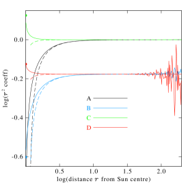
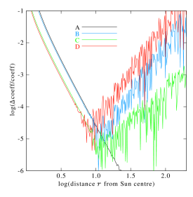
Figure 5: Radial variation of Minnaert’s coefficients $A$, $B$, $C$ and $D$ with distance from the solar centre. Asymptotically, the coefficients decrease as $r^{-2}$, the left diagram therefore shows the coefficients multiplied with $r^{2}$. The dashed curves represent the respective asymptotic expansions. The coloured dots on the ordinate represents the respective value for $r=R_{\odot}$ except for $A(r=R_{\odot})=0$. In the right diagram we display the logarithm of the absolute relative difference between the coefficients calculated in single precision and the asymptotic approximation.

In the left diagram of Fig. 5 we show the variation of Minnaert’s coefficients with distance $r$. For comparison, their respective asymptotic series expansion as derived in chapter A.4 of the appendix is also displayed (dashed). For large $r$ all coefficients have to decrease as $r^{-2}$ to reproduce the analogous decrease of the solar radiation at distances for which the Sun can be treated as a point source. At these large distances, the coefficients, especially $B$ and $D$, are prone to numerical roundoff errors. These numerical errors are even more dominant when the radial polarisation $I_{\mathrm{rad}}$ is calculated for which the combinations $C-A$ and $D-B$ of the coefficients are required which decrease as $r^{-4}$. In the right diagram we show the relative error between the coefficients and their asymptotic expansions. The error below $r\simeq 10R_{\odot}$ is caused by the insufficient expansion which takes only the two lowest order terms into account. Above $r\simeq 10R_{\odot}$ the error is due to the numerical instability of the full expressions for the coefficients $B$, $D$ and $C$ (here calculated with single precision). In view of the fact that the asymptotic terms are also much simpler to calculate, we suggest to switch to the latter when the argument $r$ exceeds about $10\;R_{\odot}$.

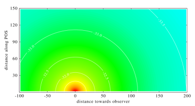
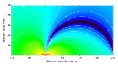
Figure 6: Radiant intensities $I_{\mathrm{tan}}$ (top) and $I_{\mathrm{rad}}$ (bottom) Thomson scattered from a single electron and polarised in tangential and radial direction. The distribution of the radiant intensities is displayed in the mean scattering plane according to (3.37) and (3.38), respectively. The Sun is at the origin, the spatial units are $R_{\odot}$, the observer is assumed at (200,0) $R_{\odot}$. The contour labels refer to the decadic logarithm of the radiant intensity [W/sr] for a unit mean solar radiance, i.e., setting $L_{\odot}=(1-u/3)^{-1}$ W/m²/sr.

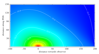
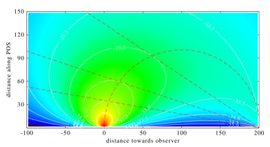
Figure 7: Total and polarised radiant intensities $I_{\mathrm{tan}}+I_{\mathrm{rad}}$ and $I_{\mathrm{tan}}-I_{\mathrm{rad}}$, respectively, Thomson scattered from a single electron. Parameters are as in Fig. 6, in particular the Sun is at the origin, the spatial units are $R_{\odot}$ and the observer is assumed at (200,0) $R_{\odot}$.

In Fig. 6 we show the spatial distribution of the radiant intensity scattered from a single electron in the mean scattering plane around the Sun. The contours of the tangential component $I_{\mathrm{tan}}(\mathbfl{r})$ (upper panel) are concentric around the Sun because it does not depend on the mean scattering angle $\bar{\chi}$ but only on the radial distance $r$. This is different for $I_{\mathrm{rad}}(\mathbfl{r})$ (lower panel) which for $\bar{\chi}=\pi/2$ only represents the small radial $Q_{\mathrm{sc},zz}$ component (see eqs.  3.17 and 3.18) of the Sun’s incident irradiance. The latter is due to the Sun’s finite apparent size and $Q_{\mathrm{sc},zz}$ rapidly decreases with distance $r$. The condition $\bar{\chi}=\pi/2$ defines the “Thomson scattering sphere” [Vourlidas and Howard, 2006]. In the spatial distribution $I_{\mathrm{rad}}$ this surface is marked by a deep depletion.

This minimum of $I_{\mathrm{rad}}$ is filled by forming combinations of $I_{\mathrm{tan}}$ and $I_{\mathrm{rad}}$ which are shown in Fig. 7. Here we display the combinations $I_{\mathrm{rad}}\pm I_{\mathrm{rad}}$, the total ($+$) and the polarised ($-$) components of the radiant intensity. For $I_{\mathrm{tot}}$, the depletion of $I_{\mathrm{rad}}$ at $\bar{\chi}=\pi/2$ leads to a flattening of the contours at this mean scattering angle, while $I_{\mathrm{pol}}$ is naturally suppressed in the forward and backward scattering direction, i.e. at $\bar{\chi}=0$ and $\pi/2$. At these scattering angles the tangential and radial polarisations become indistinguishable and $I_{\mathrm{tan}}$ and $I_{\mathrm{rad}}$ become equal. A halo-CME might be considerably dimmed in polarised brightness relative to the near-Sun coronal background and it should be much better visible in radial polarisation. The exact limits $\bar{\chi}=0$ or $\pi$ are, of course, hidden behind a coronagraph by the occulter.

When the observer receives a signal from a certain line-of-sight he in general does not know how $N_{e}(\mathbfl{r}(\ell))$ is distributed. With the distribution of the radiant intensity as the only a-priori information at hand, we might be tempted to argue that the most probable scattering site is where $I(\mathbfl{r}(\ell))$ maximises for this line-of-sight as function of $\ell$. It is easily confirmed that the radiant intensity for all polarisations except $I_{\mathrm{rad}}$ maximises at a point near $\bar{\chi}=\pi/2$. The locus of these points agrees therefore with the Thomson sphere mentioned above. In the bottom diagram of Fig. 7 we have drawn as an example three such lines-of-sights as dashed lines from the observer at (200,0) and the Thomson sphere as a dashed circle. The line-of-sight beams tangentially touch the contour of their highest radiant intensity at the Thomson sphere. In this way, $\bar{\chi}=\pi/2$ is defined graphically as the locus of the largest scattering probability on each individual line-of-sight. From the distance between the line-of-sight and its maximum intensity contour at $\bar{\chi}=\pi/2$ we can infer the slow decrease of the radiant intensity from its maximum along a line-of-sight. It is obviously much slower for $I_{\mathrm{tot}}$ than for $I_{\mathrm{pol}}$ as was noted by Howard and DeForest [2012]. They also pointed out that the reason for the maximum of the radiant intensity on the Thomson sphere is its comparatively rapid radial decrease which can be traced back to the $r$-dependence of Minnaert’s coefficients. It therefore does not reflect any peculiarity of Thomson scattering.

It is difficult to say how much significance the Thomson sphere has for practical observations. It has to be kept in mind, that the respective radiant intensity per electron must still be multiplied with the density $N_{e}$ before the line-of-sight signal can be integrated. The fact that the density can vary by orders of magnitude considerably reduces the relevance of the line-of-sight variation of the radiant intensity. Moreover, the radiant intensity also decreases in radial direction. A plasma cloud propagating away from the Sun with $\bar{\chi}$ well away from $\pi/2$ produces a somewhat attenuated scattering signal and will therefore be visible out to a slightly shorter radial distance until its brightness contrast is drowned in noise. A propagation well off the Thomson sphere will therefore probably not completely prevent the detection of the cloud.

4 Integration of simple coronal density models

Figure 8: Geometry of the line-of-sight. We use two alternative length parameters along the line-of-sight: $\ell$ is the distance from the observer, $s$ is the distance from the point of closest approach of the line-of-sight to the Sun. The angle $\bar{\chi}$ is the mean scattering angle at the scattering site $\mathbfl{r}$.

In some simple cases, the line-of-sight integrals (3.41) can be calculated analytically but in most practical cases numerical methods are needed. Either way, the line-of-sight integration should be arranged suitably. For that purpose we replace the line-of-sight parameter $\ell$ by a new parameter $s$ which measures the (signed) geometrical distance along the line-of-sight from the point of closest approach to the solar centre at $\bar{\chi}=\pi/2$. The new line-of-sight parameter $s=\ell+s_{\mathrm{obs}}$ ranges from $s=s_{\mathrm{obs}}<0$ to $s\rightarrow+\infty$. The distance of the line-of-sight at $s=0$ from the solar centre is $\rho$. Then we have the following relations between $s$ and $\bar{\chi}$ along a line-of-sight specified by either $\rho$ or $\varepsilon$ (see Fig. 8)

$$\begin{gathered}r=\sqrt{\rho^{2}+s^{2}},\qquad s=-r\cos\bar{\chi},\qquad\rho=r\sin\bar{\chi}\\ \text{especially},\;s_{\mathrm{obs}}=-r_{\mathrm{obs}}\cos\varepsilon,\qquad r_{\mathrm{obs}}=\rho/\sin\varepsilon\end{gathered}$$ (4.1)

Here $r_{\mathrm{obs}}$ is the distance of the observer from the Sun centre and $\varepsilon$ is the elongation of the line-of-sight path as seen from the observer. In (3.41) we have to read $r$ and $\bar{\chi}$ as functions of $s$ and the line-of-sight constant $\rho$

$$r(s)=\sqrt{\rho^{2}+s^{2}},\qquad\bar{\chi}(s)=\mathrm{acos}(\frac{s}{r(s)})$$

For practical calculations we want avoid the infinite upper integration boundary of $s$. We therefore substitute $s\longrightarrow\bar{\chi}$ as integration variable. The Jacobian of this variable transformation is

$$\frac{ds}{d\bar{\chi}}=-(\frac{dr}{d\bar{\chi}})\cos\bar{\chi}+r\sin\bar{\chi}=-\rho(\frac{d}{d\bar{\chi}}\frac{1}{\sin\bar{\chi}})\cos\bar{\chi}+\rho=\rho(\frac{\cos^{2}\bar{\chi}}{\sin^{2}\bar{\chi}}+1)=\frac{\rho}{\sin^{2}\bar{\chi}}$$ (4.2)

We insert the Minnaert expressions (3.37) and (3.38) for the radiant intensities in the integrand of (3.41) with $r(\bar{\chi})=\rho/\sin\bar{\chi}$ and use the above variable transformation to express $N_{e}(\mathbfl{r}(\ell))=N_{e}(r,\bar{\chi})$. Then the observed radiant fluxes (3.41) into a pixel in various polarisations read

$$\Phi_{\mathrm{p}}=\frac{A_{\mathrm{aperture}}A_{\mathrm{pixel}}}{f^{2}}\;\frac{\pi r_{e}^{2}L_{\odot}}{2}K_{\mathrm{p}}(\rho)\quad\text{for p=``tan'', ``rad'', ``pol'', ``tot''}$$ (4.3)

$$K_{\mathrm{tan}}(\rho)=\rho\int_{\varepsilon}^{\pi}N_{e}(r,\bar{\chi})\;((1-u)C(r)+uD(r))\;\frac{d\bar{\chi}}{\sin^{2}\bar{\chi}}\qquad[\mathrm{1/m^{2}}]$$

$$K_{\mathrm{pol}}(\rho)=\rho\int_{\varepsilon}^{\pi}N_{e}(r,\bar{\chi})\;((1-u)A(r)+uB(r))\;d\bar{\chi}$$

$$K_{\mathrm{tot}}=2K_{\mathrm{tan}}-K_{\mathrm{pol}},\qquad K_{\mathrm{rad}}=K_{\mathrm{tan}}-K_{\mathrm{pol}}$$

$$\text{where}\quad r(\bar{\chi})=\frac{\rho}{\sin\bar{\chi}}\quad\text{has to be used in the integrands}$$

These equations will serve as the basis for the numerical and analytical line-of-sight integrations below.

4.1 Axially symmetric coronal density

To simplify the above integrations in (4.3) we will make two assumptions in this section:
       1) $N_{e}(r,\bar{\chi})$ only depends on the distance from the solar centre $r$
       2) we approximate the lower integration boundary in (4.3) by $\varepsilon=0$ assuming an infinite distance $r_{\mathrm{obs}}$ of the observer.
Condition 1 may be relaxed in that the dependence $N_{e}(r)$ may differ in each azimuthal scattering plane. However, even this assumption is unrealistic for the coronal density distribution at a given time. Yet it sometimes may be meaningful when a long time mean or background density is considered [Hayes et al., 2001, Quémerais and Lamy, 2002]. Since (3.41) is linear in density $N_{e}$, any averaging of coronagraph images is likewise implicitly applied to the density $N_{e}(r)$. This way image data can be generated for which the averaged $N_{e}$ may come close to condition 1.

Condition 2 may be satisfied by an appropriate combination of measured data if we add to the radiant flux per pixel $\Phi(\varepsilon)$ observed at finite distance $r_{\mathrm{obs}}$ the data from $\Phi(\pi-\varepsilon)$ observed in the exact opposite direction. Since the dependence of the integrand on the mean scattering angle $\bar{\chi}$ is only through $\sin\bar{\chi}=\sin(\pi-\bar{\chi})$, the sum of these observations represents the integral over the entire line-of-sight from $s=-\infty$ to $+\infty$ or from a virtual space craft at infinite distance from Sun made at $\varepsilon\simeq 0$. In most cases, e.g., for observations from a distance of 1 AU, these “anti-sunward” observations $\Phi(\pi-\varepsilon)$ will not be considered to make a significant contribution and condition 2 is therefore not very restrictive.

Accepting the above assumptions, the integration (4.3) becomes equivalent to an Abel transformation we denote by $f(\rho)=\mathcal{A}(g(r))$ (see chapter B in the appendix). Multiplying $1=(\rho/r\sin\bar{\chi})^{2}$ to the integrand of $K_{\mathrm{pol}}$ of (4.3), we can write the line-of-sight integrals as

$$K_{\mathrm{tan}}(\rho)=\mathcal{A}[N_{e}(r)\;((1-u)C(r)+uD(r))]$$ (4.4)

$$K_{\mathrm{pol}}(\rho)=\;\rho^{2}\;\mathcal{A}[N_{e}(r)\;\frac{(1-u)A(r)+uB(r)}{r^{2}}]$$ (4.5)

The inversion of the two above Abel transforms independently yields the density $N_{e}(r)$ from the two polarisation observations $K_{\mathrm{tan}}$ and $K_{\mathrm{pol}}$ by

$$N_{e}(r)=\frac{1}{(1-u)C(r)+uD(r)}\;\mathcal{A}^{-1}[K_{\mathrm{tan}}(\rho)]$$

$$\hskip 34.44434pt=\frac{r^{2}}{(1-u)A(r)+uB(r)}\;\mathcal{A}^{-1}[\frac{K_{\mathrm{pol}}(\rho)}{\rho^{2}}]$$ (4.6)

In principle, this relation could serve as a check of the assumption that $N_{e}$ has spherical symmetry. For real measurements, however, (4.6) is never satisfied because both, $K_{\mathrm{tan}}(\rho)$ and $K_{\mathrm{pol}}(\rho)$, are contaminated by Rayleigh scattering and defraction at dust particles and stray light produced inside the instrument [Koutchmy and Lamy, 1985, Llebaria et al., 2010]. The latter two contributions are often assumed unpolarised and therefore contribute only to $K_{\mathrm{tan}}(\rho)$. Rayleigh scattering at irregularly formed dust particles has an increasing polarisation with scattering angles deviating from forward scattering. As a result, it yields a non-negligible contribution also to $K_{\mathrm{pol}}(\rho)$ at distances $\rho>4$ to 5 $R_{\odot}$ [e.g., Levasseur-Regourd et al., 2001]. In many studies, (4.6) is therefore rather used to separate the Thomson scattered signal (K-corona) from the Rayleigh scattered contribution (F-corona) and from instrument stray light. Another way to distinguish the Thomson scattered part from the rest is by spectroscopy. The large Doppler shift in scattering at fast electrons smears out the Fraunhofer lines which remain detectable in the other contributions.

Figure 9: The polarisation degree from a spherically symmetric electron corona with a density $N_{e}(r)=N(R_{\odot}/r)^{-\gamma}$ for different values of $\gamma$. The formal limit $\gamma\rightarrow\infty$ can of of course never be observed because the rapid drop of the density for large $\gamma$ eventually reduces the absolute signal strength below measurability.

Some additional considerations how to calculate the inverse Abel transformation numerically and analytically can be found in appendix B. As a simple application, let us determine the polarisation degree for a power-law coronal electron density. This was already treated by [Van de Hulst, 1950]. Even Schuster [1879] made the first calculations of this ratio because it is independent from the then unknown scattering cross section and the radial dependence of the polarisation degree was a first test of the scattering theory in those days. Because of the complex radial dependence of the Minnaert’s coefficients in (4.4) and (4.5), the integrals still have to be evaluated numerically, but at a large enough distance $r$ we can use the asymptotic dependence for the Minnaert coefficients (see chapter A.5 in the appendix)

$$(1-u)C(r)+uD(r)\xrightarrow{\rho\rightarrow\infty}(1-u/3)L_{\odot}(\frac{R_{\odot}}{r})^{2}$$

$$(1-u)A(r)+uB(r)\xrightarrow{\rho\rightarrow\infty}(1-u/3)L_{\odot}(\frac{R_{\odot}}{r})^{2}$$

If we further assume a power law dependence for the density of $N_{e}(r)=N(R_{\odot}/r)^{-\gamma}$ we find

$$K_{\mathrm{tan}}(\rho)\xrightarrow{\rho\rightarrow\infty}(1-u/3)L_{\odot}NR_{\odot}^{2+\gamma}\mathcal{A}[\frac{1}{r^{2+\gamma}}]$$

$$K_{\mathrm{pol}}(\rho)\xrightarrow{\rho\rightarrow\infty}(1-u/3)L_{\odot}NR_{\odot}^{2+\gamma}\rho^{2}\mathcal{A}[\frac{1}{r^{4+\gamma}}]$$

For the Abel transform of a power law we have (see chapter B.1 in the appendix)

$$\mathcal{A}(r^{-\alpha})=\frac{2\pi}{\alpha-1}\frac{1}{\displaystyle B(\frac{\alpha}{2},\frac{1}{2})}\rho^{1-\alpha},\quad\mathcal{A}^{-1}(\rho^{-\beta})=\frac{\beta}{2\pi}B(\frac{\beta+1}{2},\frac{1}{2})r^{-1-\beta}$$

where $B(x,y)$ is the beta function (B.10). This yields

$$K_{\mathrm{tan}}(\rho)\xrightarrow{\rho\rightarrow\infty}(1-u/3)L_{\odot}NR_{\odot}^{2+\gamma}\frac{2\pi}{\gamma+1}\frac{1}{B(\frac{\gamma+2}{2},\frac{1}{2})}\rho^{-\gamma-1}$$

$$K_{\mathrm{pol}}(\rho)\xrightarrow{\rho\rightarrow\infty}(1-u/3)L_{\odot}NR_{\odot}^{2+\gamma}\frac{2\pi}{\gamma+3}\frac{1}{B(\frac{\gamma+4}{2},\frac{1}{2})}\rho^{-\gamma-1}$$

$$\frac{K_{\mathrm{tan}}}{K_{\mathrm{pol}}}\xrightarrow{\rho\rightarrow\infty}\frac{\gamma+3}{\gamma+1}\frac{B(\frac{\gamma+4}{2},\frac{1}{2})}{B(\frac{\gamma+2}{2},\frac{1}{2})}=\frac{\gamma+3}{\gamma+1}\frac{\Gamma(\frac{\gamma+4}{2})}{\Gamma(\frac{\gamma+5}{2})}\frac{\Gamma(\frac{\gamma+3}{2})}{\Gamma(\frac{\gamma+2}{2})}=\frac{\gamma+3}{\gamma+1}\frac{\frac{\gamma+2}{2}}{\frac{\gamma+3}{2}}=\frac{\gamma+2}{\gamma+1}$$

For the asymptotic polarisation degree we find

$$P=\frac{K_{\mathrm{pol}}}{K_{\mathrm{tot}}}=\frac{K_{\mathrm{pol}}}{2K_{\mathrm{tan}}-K_{\mathrm{pol}}}=\frac{1}{2\frac{K_{\mathrm{tan}}}{K_{\mathrm{pol}}}-1}=\frac{\gamma+1}{2(\gamma+2)-\gamma-1}=\frac{\gamma+1}{\gamma+3}$$ (4.7)

In Fig. 9 we show the degree $P$ of a mere electron corona as function of the line-of-sight distance $\rho$ for different power laws of the coronal density. The polarisation degree is calculated from (4.4) and (4.5), their asymptotic value (4.7) is marked by a horizontal line. Again, the measured polarisation degree differs from Fig. 9 [e.g., Saito et al., 1970, Koutchmy and Lamy, 1985, Badalyan et al., 1993] because of additional contributions from scattering at dust and from instrument stray light. Since the electron density drops rapidly with distance from the Sun, the relative influence of these additional sources increase with distance. They contribute mainly to the unpolarised signal and as a result the measured polarisation degree drops with distance $\rho$ beyond 1.5 to 2 $R_{\odot}$.

4.2 CME-like density perturbation

In this section discuss the observation of a CME-like density perturbation and how a varying width of the CME may modify our estimate of its propagation direction, its column mass density and of the entire CME mass. From a single image alone, the width of a CME in heliographic longitude cannot be perceived. Attempts have been made to use two (or more) images from the STEREO space craft from different perspectives or to use two different polarisations from a single perspective to make a guess of the propagation direction and the width of a CME [e.g., Mierla et al., 2011]. As the width estimate often rather crude, so will be our CME model.

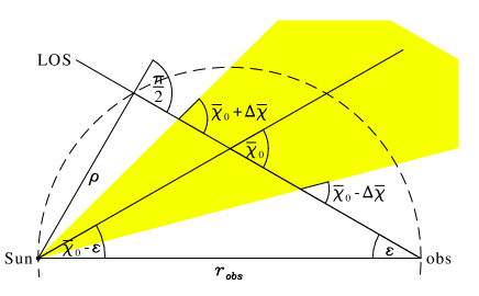
Figure 10: Geometry of the model CME discussed in the text. The CME centre propagates from the Sun at the lower left at an angle $\bar{\chi}_{0}-\varepsilon$ with respect to the Sun-observer line. The CME cone of width $\pm\Delta\bar{\chi}$ around the CME centre axis is shaded in yellow. The line-of-sight starting at the observer (at the lower right) makes an angle of the elongation $\varepsilon$ with the Sun-observer line.

We assume for a given line-of-sight at elongation $\varepsilon$ (see Fig. 10) a CME the centre of which crosses the line-of-sight at a central mean scattering angle $\bar{\chi}_{0}$. Along the line-of-sight, the electron density may be distributed like a Gaussian in the variable $\bar{\chi}-\bar{\chi}_{0}$ with width $\Delta\bar{\chi}$. In the case that the background has been successfully eliminated from observed data by forming difference images, the density perturbation responsible for the residual signal power is then

$$N_{e}(r,\bar{\chi})=N_{0}\frac{R^{2}_{\odot}}{r^{2}}g(\bar{\chi};\bar{\chi}_{0},\Delta\bar{\chi}),\quad g(\bar{\chi};\bar{\chi}_{0},\Delta\bar{\chi})=\frac{1}{\sqrt{\pi}\Delta\bar{\chi}}\exp(-(\frac{\bar{\chi}-\bar{\chi}_{0}}{\Delta\bar{\chi}})^{2})$$ (4.8)

where we used once again $r=\rho/\sin\bar{\chi}$. This model CME has a column density integral of

$$n_{\mathrm{col}}=\int_{-\infty}^{\infty}N_{e}(r,\bar{\chi})\;ds=N_{0}\int_{-\infty}^{\infty}\frac{R^{2}_{\odot}\sin^{2}\bar{\chi}}{\rho^{2}}g(\bar{\chi})\frac{\rho d\bar{\chi}}{\sin^{2}\bar{\chi}}$$

$$=N_{0}\frac{R^{2}_{\odot}}{\rho}\int_{-\infty}^{\infty}g(\bar{\chi})\;d\bar{\chi}=N_{0}\frac{R^{2}_{\odot}}{\rho}\qquad[\mathrm{1/m^{2}}]$$ (4.9)

Its geometry is sketched in Fig. 10. For $\bar{\chi}_{0}=\pi/2$ the intersection of the CME centre with the line-of-sight is located on the Thomson sphere, for $\bar{\chi}_{0}<\pi/2$ it is inside and for $\bar{\chi}_{0}>\pi/2$ it is outside of the Thomson sphere. The CME propagation angle with respect to the Sun-observer line is $\bar{\chi}_{0}-\varepsilon=\bar{\chi}_{0}-\mathrm{asin}(\rho/r_{\mathrm{obs}})$.

The line-of-sight integrations to be performed in (4.3) are then

$$K_{\mathrm{tan}}(\rho)=N_{0}R^{2}_{\odot}\rho\int_{\varepsilon}^{\pi}((1-u)C(r)+uD(r))\;g(\bar{\chi})\;\frac{d\bar{\chi}}{r^{2}\sin^{2}\bar{\chi}}$$

$$=n_{\mathrm{col}}\int_{\varepsilon}^{\pi}((1-u)C(r)+uD(r))\;g(\bar{\chi})\;d\bar{\chi}$$ (4.10)

$$K_{\mathrm{pol}}(\rho)=N_{0}R^{2}_{\odot}\rho\int_{\varepsilon}^{\pi}((1-u)A(r)+uB(r))\;g(\bar{\chi})\;\frac{d\bar{\chi}}{r^{2}}$$

$$=n_{\mathrm{col}}\int_{\varepsilon}^{\pi}((1-u)A(r)+uB(r))\;g(\bar{\chi})\sin^{2}\bar{\chi}\,d\bar{\chi}$$ (4.11)

where we used again $r\sin\bar{\chi}=\rho$. For $\Delta\bar{\chi}\rightarrow 0$ these expressions become independent on the special shape function $g(\bar{\chi})$

$$\lim_{\Delta\bar{\chi}\rightarrow 0}K_{\mathrm{tan}}=n_{\mathrm{col}}\;((1-u)C(\frac{\rho}{\sin\bar{\chi}_{0}})+uD(\frac{\rho}{\sin\bar{\chi}_{0}}))$$

$$\lim_{\Delta\bar{\chi}\rightarrow 0}K_{\mathrm{pol}}=n_{\mathrm{col}}\;((1-u)A(\frac{\rho}{\sin\bar{\chi}_{0}})+uB(\frac{\rho}{\sin\bar{\chi}_{0}}))\sin^{2}\bar{\chi}_{0}$$

and given that $\bar{\chi}_{0}$ is known the observations can be inverted to yield an estimate of the column density $n_{\mathrm{col}}$. These relations have often been used for CME mass estimates which are obtained by summing the column densities pixel by pixel and multiplying with a mean coronal ion mass per electron charge.

Figure 11: Plot of $K(\bar{\chi}_{0},\Delta\bar{\chi},\rho)$ for a CME cone with Gaussian cross section vs the propagation angle $\bar{\chi}_{0}-\varepsilon$ of the CME and for different widths $\Delta\bar{\chi}$. The widths are varied from $\Delta\bar{\chi}=$ 0^∘ to 60^∘ in steps of 10^∘ and the line-of-sight distance to the solar centre was chosen to $\rho=$ 5 $R_{\odot}$. The $K$-values are normalised by $K(\rho,\pi/2,0)$ of a CME density concentrated entirely on the Thomson sphere. The left diagram displays the total signal, the right diagram the polarised signal.

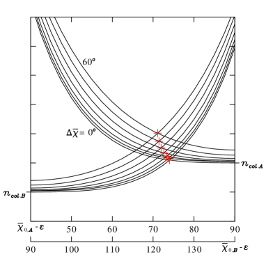
Figure 12: Example of the determination of the propagation angle and a consistent column mass density from the observation of $K_{\mathrm{tot}}$ form two vantage points $A$ and $B$ at $\rho=5R_{\odot}$ for both of them. The two observers are $50^{\circ}$ apart. The curves represent the column mass density obtained from $K_{\mathrm{tot}}(\rho;\bar{\chi}_{0},\Delta\bar{\chi})$ as function of the propagation angle with respect to spacecraft A (decreasing curves) and B (increasing curves) and for different assumed widths $\Delta\bar{\chi}$. $n_{\mathrm{col,A}}$ and $n_{\mathrm{col,B}}$ are the respective minimal column mass density corresponding to $K_{\mathrm{tot}}(\rho;\pi/2,0)$. The consistent propagation angle and column mass density is obtained from the intersection of the curve from A and B with the same assumed width $\Delta\bar{\chi}$. The tick marks on the ordinate are in units of 0.1 $n_{\mathrm{col,A}}$. For further an explanation see the text.

In Fig. 11 we show the total $K_{\mathrm{tot}}(\rho;\bar{\chi}_{0},\Delta\bar{\chi})$ and the polarised signal $K_{\mathrm{pol}}(\rho;\bar{\chi}_{0},\Delta\bar{\chi})$ to be observed for such an idealised CME cone on a line-of-sight with $\rho=5R_{\odot}$ (i.e., for constant elongation $\varepsilon$) and for different $\bar{\chi}_{0}$ and $\Delta\bar{\chi}$. In both cases we normalise $K(\rho;\bar{\chi}_{0},\Delta\bar{\chi})$ by the respective limit $K(\rho;\pi/2,0)$ obtained for a CME density entirely concentrated on the Thomson sphere. This choice $\bar{\chi}_{0}=\pi/2$ and $\Delta\bar{\chi}=0$ was the general assumption for CME mass estimates before the STEREO era. As noted by Vourlidas and Howard [2006] this assumption could result in a considerable underestimate of $n_{\mathrm{col}}$ when the true propagation angle $\bar{\chi}_{0}$ differs from $\pi/2$. Fig .11 shows that a neglect of a finite CME width $\Delta\bar{\chi}$ even enhances this underestimate by up to 20% when $\bar{\chi}_{0}$ is less than 50^∘ off the Thomson sphere for $K_{\mathrm{tot}}$ and less than 30^∘ off for $K_{\mathrm{pol}}$.

With the stereo information from two space craft, either the propagation direction could be determined by triangulation or by adjusting the propagation angles relative to the two space craft until the mass estimate from both space craft is consistent [Colaninno and Vourlidas, 2009]. This latter method can be applied graphically by plotting the estimated mass vs propagation angle dependence for both view points into one diagram with the propagation angles appropriately shifted by the heliospheric longitude difference of the tow observing spacecraft (assuming both space craft have the same distance from Sun). The intersection of these curves yields the consistent mass and the associated propagation angles with respect to each spacecraft. An example for such a diagram is shown in Fig. 11 for different assumed CME widths. Two observers A and B with a 50^∘ heliographic longitude difference measure $K_{\mathrm{tot}}(\rho)$ at the same $\rho=5R_{\odot}$ and corresponding to $n_{\mathrm{col,A}}$ and $n_{\mathrm{col,B}}$, respectively, under the assumption $\bar{\chi}_{0}=\pi/2$ and $\Delta\bar{\chi}=0$. The intersection for curves with the same assumed width are marked with a red cross. Each width yields a slightly different propagation direction and a different column mass estimate. If the finite width of the CME is ignored and $\Delta\bar{\chi}=0$ is assumed (lowest curves in Fig. 11), the column density could still be appreciably underestimated. The consistent propagation angle varies within $\pm 5^{\circ}$ in the idealised case treated here.

To apply this method to just a column integral is only justified here because we use an idealised cone as CME model. However, the method could in principle be extended to the sum over all pixels illuminated by a CME and the respective CME mass estimates from both view point could be used instead of the column density integrals. A slight complication arises because there is a difference between $\bar{\chi}_{0}$ and the propagation angle $\bar{\chi}_{0}-\varepsilon$. For $\rho=5R_{\odot}$ and $r_{\mathrm{obs}}=200R_{\odot}$ as in our example $\varepsilon$ is less than a degree and $\bar{\chi}_{0}$ practically agrees with the propagation angle. For larger $\varepsilon$, as they occur in heliospheric imager observations this difference cannot be neglected anymore. It varies with $\rho$ and has to be taken into account when column density integrals are summed to estimate the total CME mass.

Figure 13: Plot of the polarisation ratio $K_{\mathrm{pol}}(\bar{\chi}_{0},\Delta\bar{\chi},\rho)$ to $K_{\mathrm{tot}}(\bar{\chi}_{0},\Delta\bar{\chi},\rho)$ for a CME cone of Gaussian cross section vs the angle $\bar{\chi}_{0}-\pi/2$ off the plane of the sky for different widths from $\Delta\bar{\chi}=$ 0 to 60^∘ in steps of 10^∘ and for $\rho=$ 5 $R_{\odot}$.

A similar error could affect the polarisation ratio method [Moran and Davila, 2004] which uses the ratio $K_{\mathrm{pol}}/K_{\mathrm{tot}}$ to estimate the scattering position $|\bar{\chi}_{0}-\pi/2|$ off the Thomson sphere. For small elongations $\varepsilon$, this corresponds to the CME propagation angle off the plane of the sky. Again a vanishing CME width $\Delta\bar{\chi}$ is traditionally assumed. In Fig. 13, we display this ratio for varying cone widths. A neglect of the width could again lead to a wrong estimate of $|\bar{\chi}_{0}-\pi/2|$. E.g., a wide CME with $\Delta\bar{\chi}=60^{\circ}$ propagating at $\bar{\chi}_{0}=0$ yields a ratio of 0.8 which could be interpreted as a CME propagating at 20^∘ if the width is ignored. From Fig. 13 we see that this way the propagation angle could be overestimated by up to 20^∘ for $K_{\mathrm{pol}}/K_{\mathrm{tot}}>0.7$ and may be underestimated even more for $K_{\mathrm{pol}}/K_{\mathrm{tot}}<0.6$, all depending on the true width $\Delta\bar{\chi}$.

A major simplification of (4.10) and (4.11) is obtained if the column density integrals are evaluated on line-of-sights with large $\rho=r_{\mathrm{obs}}\sin\varepsilon$, i.e. for large spacecraft distances and sufficiently large elongations $\varepsilon$. Since $r\geq\rho$ we have from appendix A.4

$$\lim_{r\rightarrow\infty}A(r)=\lim_{r\rightarrow\infty}C(r)=\theta^{2}_{\mathrm{max}}\simeq\frac{R^{2}_{\odot}}{r^{2}},\quad\lim_{r\rightarrow\infty}B(r)=\lim_{r\rightarrow\infty}D(r)=\frac{2}{3}\theta^{2}_{\mathrm{max}}\simeq\frac{2R^{2}_{\odot}}{3r^{2}}$$

and setting $r=\rho/\sin\bar{\chi}$, we obtain

$$K_{\mathrm{tan}}(\rho)\xrightarrow{\rho\rightarrow\infty}n_{\mathrm{col}}\;(1-u/3)\frac{R^{2}_{\odot}}{\rho^{2}}\int_{\varepsilon}^{\pi}g(\bar{\chi})\sin^{2}\bar{\chi}d\bar{\chi}$$ (4.12)

$$K_{\mathrm{pol}}(\rho)\xrightarrow{\rho\rightarrow\infty}n_{\mathrm{col}}\;(1-u/3)\frac{R^{2}_{\odot}}{\rho^{2}}\int_{\varepsilon}^{\pi}g(\bar{\chi})\sin^{4}\bar{\chi}d\bar{\chi}$$ (4.13)

$$K_{\mathrm{tot}}(\rho)=2K_{\mathrm{tan}}(\rho)-K_{\mathrm{pol}}(\rho)\hskip 130.0002pt$$

$$\hskip 60.00009pt\xrightarrow{\rho\rightarrow\infty}n_{\mathrm{col}}\;(1-u/3)\frac{R^{2}_{\odot}}{\rho^{2}}\int_{\varepsilon}^{\pi}g(\bar{\chi})(1-\cos^{4}\bar{\chi})d\bar{\chi}$$ (4.14)

The interpretation of these formulas is straight forward. The factor $1-u/3$ arises because for the Sun as a point source the radiation form the entire Sun matters rather than its central radiance $L_{\odot}$ (see also eq. 3.8). The observed $K(\rho)$ effectively decreases with $\rho^{-3}$ because $n_{\mathrm{col}}\propto\rho^{-1}$ (see eq 4.9). Both the solar irradiance and the density decrease with $r^{-2}=\sin^{2}\bar{\chi}/\rho^{2}$ while the length of the line-of-sight section which intersects the CME cone grows as $\rho/\sin^{2}\bar{\chi}$ (see eq. 4.2). Together this yields the $\sin^{2}\bar{\chi}/\rho^{3}$ dependence of the tangential signal $K_{\mathrm{tan}}$. The $\bar{\chi}$ dependence of $K_{\mathrm{pol}}$ and $K_{\mathrm{tot}}$ is further modified by the additional dependence of the radiant intensity for these polarisations on the mean scattering angle through the Thomson scattering cross section Howard and DeForest [2012].

5 Electrons in motion – relativistic effects

So far, we have neglected relativistic effects. Most coronagraphs operate at optical wavelengths and integrate over a wide wavelength range. The Compton wavelength shift at these wavelengths is tiny and is only of the order of $\lambda/\lambda_{\mathrm{Compton}}=\mathcal{O}(10^{-5})$. However, even if the energy of the observed photons is small, relativistic effects may come into play due to the finite energy of the electrons. For a temperature of 10⁶ K, the ratio $\beta$ of the electron velocity to the speed of light for a thermal electron is $\mathcal{O}(10^{-2})$ which is not too far away from speeds where relativistic effects matter. Electron beams with higher energy are likely to exist in the solar corona at least sporadically close to X-ray flares and in the source region of type radio bursts.

5.1 Expected effects – a qualitative discussion

It can immediately be seen by an argument from Molodensky [1973] that a finite electron energy has an influence. Due to aberration, a relativistic electron moving to or away from the centre of the Sun will see the Sun’s size in its rest frame at a reduced or an enhanced viewing angle $\theta_{\mathrm{max}}$, respectively, compared to the value of (3.2) we found for an electron at rest. The scattering at an electron moving in one of these directions is therefore to some extent equivalent to the scattering at a stationary electron but at a different apparent distance from the Sun. Since the scattering takes place in the electron rest frame, the polarisation properties of the scattered radiation will correspond to the respective apparent distance, except that the observer will see the scattered light coming from the electron’s true (i.e., retarded) distance from the Sun in his own rest frame.

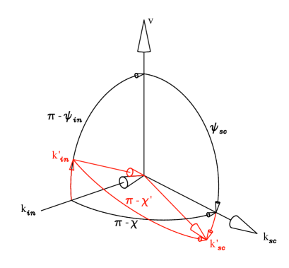
Figure 14: Illustration of the scattering of a photon at an electron moving with a relativistic velocity. The incident and scattered wave vectors are $\mathbfl{k}_{\mathrm{in}}$ and $\mathbfl{k}_{\mathrm{sc}}$, respectively. If the electron is at rest, they span the scattering plane with the scattering angle $\chi$ between them. If the electron is in motion its velocity $\mathbfl{v}$ spans two aberration planes with each of the wave vectors. The aberrated wave vectors $\mathbfl{k}^{\prime}_{\mathrm{in}}$ and $\mathbfl{k}^{\prime}_{\mathrm{sc}}$ in the electron rest frame both lie in the same respective plane. These wave vectors then span the scattering plane in the rest frame of the electron (drawn in red).

Therefore even if the photon energy is moderate in the electron rest frame and Thomson scattering applies, the transformations into and out of the electron rest frame can make a substantial difference in the energy and polarisation of the scattered photon compared to Thomson scatter at an electron at rest. Before we present the calculations in detail, we will first give a qualitative description of how to approach the problem. Consider an electron with a velocity $\mathbfl{v}=c\boldsymbol{\beta}$ in the Sun’s reference frame $S$. Let $\nu_{\mathrm{in}}$ be the frequency of the incident photon and $\psi_{\mathrm{in}}$ the angle between its propagation direction $\mathbfl{\hat{k}}_{\mathrm{in}}$ and $\mathbfl{v}$ as in Fig. 14. In general, we will denote quantities in the electron rest frame $S^{\prime}$ by a dash attached to the equivalent variable name used in the Sun’s rest frame $S$. Then $\nu^{\prime}$ and $\psi^{\prime}_{\mathrm{in}}$ are the respective parameters seen in the electron rest frame $S^{\prime}$. They transform as (see eqs. D.14 and D.11 in appendix D)

$$\nu^{\prime}=\frac{\nu_{\mathrm{in}}}{D(\mathbfl{\hat{k}}_{\mathrm{in}},\boldsymbol{\beta})}=\nu_{\mathrm{in}}\gamma(1-\beta\cos\psi_{\mathrm{in}})$$ (5.1)

$$\cos\psi^{\prime}_{\mathrm{in}}=\frac{\cos\psi_{\mathrm{in}}-\beta}{1-\beta\cos\psi_{\mathrm{in}}}$$ (5.2)

where $\gamma=1/\sqrt{1-\beta^{2}}$ is the Lorentz factor and $D(\mathbfl{\hat{k}}_{\mathrm{in}},\boldsymbol{\beta})$ is commonly called the frequency shift factor (note it is larger than one for a redshift). The maximum frequency upshift is achieved for $\psi_{\mathrm{in}}=\pi$ when $\mathbfl{k}_{\mathrm{in}}$ and $\mathbfl{v}$ are antiparallel. Then the upshift amounts to a factor $\nu^{\prime}/\nu_{\mathrm{in}}=\sqrt{(1+\beta)/(1-\beta)}$. Unless $\beta$ is close to unity, incident white light photons with a wave length around $5\;10^{-7}$ m will remain far from the Compton regime in the rest frame of the electron. For the photon momentum to matter the photon must be transformed to a wave length near $\lambda_{C}=2\pi\hbar/m_{e}c=2.4\;10^{-12}$ m equivalent to a frequency blueshift of $\nu^{\prime}/\nu_{\mathrm{in}}\simeq 2\gamma\simeq 10^{5}$. We can therefore well approximate the photon scattering in the electron rest frame $S^{\prime}$ by elastic Thomson scattering.

After being scattered, the photon has to be transformed back into the Sun’s reference frame $S$. We call $\psi_{\mathrm{sc}}$ the angle between the direction of $\mathbfl{v}$ and the direction $\mathbfl{\hat{k}}_{\mathrm{sc}}$ from the scattering site to the observer in the Sun’s rest frame. Given $\mathbfl{\hat{k}}_{\mathrm{sc}}$ and its angle $\psi_{\mathrm{sc}}$ with the electron velocity, the scattered photon transforms according to (see eqs. D.15 and D.11 in appendix D)

$$\nu_{\mathrm{sc}}=\frac{\nu^{\prime}}{D(\mathbfl{\hat{k}}_{\mathrm{sc}},-\boldsymbol{\beta})}=\nu^{\prime}\;D(\mathbfl{\hat{k}}_{\mathrm{sc}},\boldsymbol{\beta})=\frac{\nu^{\prime}}{\gamma(1-\beta\cos\psi_{\mathrm{sc}})}$$ (5.3)

$$\cos\psi^{\prime}_{\mathrm{sc}}=\frac{\cos\psi_{\mathrm{sc}}-\beta}{1-\beta\cos\psi_{\mathrm{sc}}}$$ (5.4)

The second equation determines the direction $\mathbfl{\hat{k}^{\prime}}_{\mathrm{sc}}$ into which the photon has to be scattered in the electron rest frame to reach the observer.

The geometry of the scattering process is illustrated in Fig. 14. The incident direction $\mathbfl{\hat{k}}_{\mathrm{in}}$ and $\mathbfl{v}$ span the incident aberration plane which also contains $\mathbfl{\hat{k}^{\prime}}_{\mathrm{in}}$, however, tilted with respect to $\mathbfl{\hat{k}}_{\mathrm{in}}$ according to (5.2). Similarly, we have a scattering aberration plane formed by $\mathbfl{\hat{k}}_{\mathrm{sc}}$ and $\mathbfl{v}$ also containing $\mathbfl{\hat{k}^{\prime}}_{\mathrm{sc}}$. These planes differ in general from the scattering plane formed by $\mathbfl{\hat{k}}_{\mathrm{in}}$ and $\mathbfl{\hat{k}}_{\mathrm{sc}}$ unless $\mathbfl{v}$ lies in the scattering plane. Except for this latter case, the scattering plane in the electron’s rest frame formed by $\mathbfl{\hat{k}}^{\prime}_{\mathrm{in}}$ and $\mathbfl{\hat{k}}^{\prime}_{\mathrm{sc}}$ is inclined with respect to the scattering plane in the Sun’s rest frame. Since the former plane (drawn in red in Fig. 14) is relevant for the scattering process, the observed polarisation in the Sun’s reference frame is in general inclined with respect to an observation with the electron at rest.

The total observed frequency shift from (5.1) and (5.3) is

$$\nu_{\mathrm{sc}}=\nu_{\mathrm{in}}\frac{1-\beta\cos\psi_{\mathrm{in}}}{1-\beta\cos\psi_{\mathrm{sc}}}=\nu_{\mathrm{in}}\frac{D(\mathbfl{\hat{k}}_{\mathrm{sc}},\boldsymbol{\beta})}{D(\mathbfl{\hat{k}}_{\mathrm{in}},\boldsymbol{\beta})}$$ (5.5)

Whether the frequency is red- or blueshifted depends on the angles $\psi_{\mathrm{in}}$ and $\psi_{\mathrm{sc}}$. The locus of electron velocities $\boldsymbol{\beta}$ which produce a given Doppler shift $\Delta\nu=\nu_{\mathrm{sc}}-\nu_{\mathrm{in}}$ is given by the plane in velocity space

$$\boldsymbol{\beta}^{\mathsf{T}}(\nu_{\mathrm{sc}}\mathbfl{\hat{k}}_{\mathrm{sc}}-\nu_{\mathrm{in}}\mathbfl{\hat{k}}_{\mathrm{in}})=\Delta\nu$$ (5.6)

The planes for different $\Delta\nu$ are not parallel but all planes intersect along the line given by $\boldsymbol{\beta}^{\mathsf{T}}\mathbfl{\hat{k}}_{\mathrm{sc}}=\boldsymbol{\beta}^{\mathsf{T}}\mathbfl{\hat{k}}_{\mathrm{in}}=1$. Hence, any real particle with $\beta<1$ produces a unique Doppler shift. It turns out that the headlight effect makes the scattering of photons in an upshift direction much more probable than in a direction which downshifts the frequency (for the headlight or searchlight effect, see appendix D). If we assume an isotropic distribution of incident photons, the scattering electron will see the photons coming preferentially from ahead. But Thomson scattering is only mildly anisotropic so that the photons are scattered again more or less isotropically in the electron rest frame. In the lab frame, however, these photons appear beamed preferentially in forward direction. For $\beta$ close to unity this effect is very pronounced and we can estimate the mean Doppler shift factor by integrating (5.5) over the entire sphere of unit directions $\mathbfl{\hat{k}}_{\mathrm{in}}$ while we confine $\psi_{\mathrm{sc}}$ to about zero. We then obtain as an estimate for the mean frequency shift

$$\frac{\nu_{\mathrm{sc}}}{\nu_{\mathrm{in}}}\simeq\frac{2\pi}{4\pi}\int_{-\pi}^{\pi}\frac{1-\beta\cos\psi_{\mathrm{in}}}{1-\beta}\sin\psi_{\mathrm{in}}d\psi_{\mathrm{in}}=\frac{(1+\beta)}{2(1-\beta^{2})}\int_{-1}^{1}(1-\beta\cos\psi_{\mathrm{in}})d\cos\psi_{\mathrm{in}}\simeq 2\gamma^{2}$$

For $\beta\rightarrow 1$, the Lorentz factor may greatly exceed unity and the photons are on average strongly blueshifted (inverse Compton effect). By repeated scattering the photon energy may rise eventually until Thomson scattering in the electron frame becomes invalid. Thomson scattering then has to be replaced by the more general Compton scattering process which takes proper account of the momentum and energy exchange between electron and photon. This way the cold photons and hot electrons may eventually come to an equilibrium. The inverse Compton process occurs in hot coronae of, e.g., active galactic nuclei but neither multiple scattering nor a huge $\gamma$ are likely in the solar corona.

5.2 The details – a quantitative treatment

A quantitative evaluation of the radiant intensity in the case that the scattering electron has a relativistic velocity proceeds similarly as for the electron at rest. We recall that for the case $\beta=0$ in chapter 3.2 the irradiance at a distance $r$ from the solar centre was (3.15)

$$\mathbfl{Q}_{\mathrm{in}}(r)=\int_{\Omega(r)}\mathbfl{L}(\mathbfl{\hat{k}}_{\mathrm{in}})\;d\Omega(\mathbfl{\hat{k}}_{\mathrm{in}})$$ (5.7)

where the integration over $\Omega(r)$ covers all photon propagation directions $\mathbfl{\hat{k}}_{\mathrm{in}}$ from the solar surface which can directly reach the scattering site $\mathbfl{r}$. The radiance matrix of each beam of the unpolarised radiation from the solar surface was expressed in terms of two mutually orthogonal polarisation vectors $\mathbfl{\hat{e}}_{1}$ and $\mathbfl{\hat{e}}_{2}$ normal to $\mathbfl{\hat{k}}_{\mathrm{in}}$ as

$$\mathbfl{L}(\mathbfl{\hat{k}}_{\mathrm{in}})=\frac{L(\mathbfl{\hat{k}}_{\mathrm{in}})}{2}(\mathbfl{\hat{e}}_{1}{\mathbfl{\hat{e}}_{1}}^{\mathsf{T}}+\mathbfl{\hat{e}}_{2}{\mathbfl{\hat{e}}_{2}}^{\mathsf{T}})=\frac{L(\mathbfl{\hat{k}}_{\mathrm{in}})}{2}(\boldsymbol{1}-\mathbfl{\hat{k}}_{\mathrm{in}}{\mathbfl{\hat{k}}}^{\mathsf{T}}_{\mathrm{in}})$$ (5.8)

Here $L(\mathbfl{\hat{k}}_{\mathrm{in}})$ is the scalar radiance (3.4) of the visible solar disk in the Sun’s rest frame in the direction $\mathbfl{\hat{k}}_{\mathrm{in}}$ to the scattering site $\mathbfl{r}$ which makes an angle $\zeta$ with the local solar surface normal. This was our approach in (3.1) and (3.15). The integration over the visible solar surface was performed in a spherical coordinate system centred at $\mathbfl{r}$ and with its zenith axis through the centre of the Sun so that the integration became analytically tractable.

In the case of a moving electron, we need the irradiance in the rest frame of the electron. This is the same as above, however, all variables have to be transformed into the electron rest frame, i.e.,

$$\mathbfl{Q^{\prime}}_{\mathrm{in}}=\int_{\Omega^{\prime}}\mathbfl{L}^{\prime}(\mathbfl{\hat{k}^{\prime}}_{\mathrm{in}})\;d\Omega^{\prime}(\mathbfl{\hat{k}^{\prime}}_{\mathrm{in}})$$ (5.9)

The direction vectors $\mathbfl{\hat{k}^{\prime}}_{\mathrm{in}}$ in the electron rest frame and $\mathbfl{\hat{k}}_{\mathrm{in}}$ in the Sun’s rest frame are related by aberration (D.21). Likewise, $\Omega^{\prime}$ denotes the aberrated solid angle of feasible directions $\mathbfl{\hat{k}^{\prime}}_{\mathrm{in}}$ and $\mathbfl{L}^{\prime}(\mathbfl{\hat{k}^{\prime}}_{\mathrm{in}})$ is the radiance of an unpolarised beam incident in direction $\mathbfl{\hat{k}^{\prime}}_{\mathrm{in}}$ from the solar surface to the electron, however, transformed to the electron rest frame. The incident beam is unpolarised as in the Sun’s rest frame but the polarisation plane is tilted according to the aberrated propagation direction such that the polarisation base vectors $\mathbfl{\hat{e}^{\prime}}_{1}$ and $\mathbfl{\hat{e}^{\prime}}_{2}$ are orthogonal to $\mathbfl{\hat{k}^{\prime}}_{\mathrm{in}}$ (see Cocke and Holm [1972] or chapter D.4 in the appendix). Then like (5.8) above we have

$$\mathbfl{L}^{\prime}(\mathbfl{\hat{k}^{\prime}}_{\mathrm{in}})=\frac{L^{\prime}(\mathbfl{\hat{k}^{\prime}}_{\mathrm{in}})}{2}(\mathbfl{\hat{e}^{\prime}}_{1}{\mathbfl{\hat{e}^{\prime}}_{1}}{}^{\mathsf{T}}+\mathbfl{\hat{e}^{\prime}}_{2}{\mathbfl{\hat{e}^{\prime}}_{2}}{}^{\mathsf{T}})=\frac{L^{\prime}(\mathbfl{\hat{k}^{\prime}}_{\mathrm{in}})}{2}(\boldsymbol{1}-\mathbfl{\hat{k}^{\prime}}_{\mathrm{in}}\mathbfl{\hat{k}^{\prime}}{{}^{\mathsf{T}}_{\mathrm{in}}})$$ (5.10)

In the appendix (chapter D.5) we illustrate how the shape $\Omega^{\prime}(\mathbfl{\hat{k}}^{\prime}_{\mathrm{in}})$ and the apparent radiance distribution $L^{\prime}(\mathbfl{\hat{k}}^{\prime}_{\mathrm{in}})$ from the solar surface change with increasing $\beta$. The scalar radiance in the electron frame is related to the respective distribution in the Sun’s rest frame by the transformation (see e.g., McKinley [1980], Eriksen and Grøn [1992], Weiskopf et al. [1999] or chapter D.5 in the appendix)

$$L^{\prime}(\mathbfl{\hat{k}^{\prime}}_{\mathrm{in}})=\frac{L(\mathbfl{\hat{k}}_{\mathrm{in}})}{D^{4}(\mathbfl{\hat{k}}_{\mathrm{in}},\boldsymbol{\beta})}$$ (5.11)

where $D$ is the frequency shift factor (5.1) and $L(\mathbfl{\hat{k}}_{\mathrm{in}})$ is the scalar radiance distribution (5.8) in the Sun’s rest frame.

Upon substituting the integration variable $\mathbfl{\hat{k}^{\prime}}_{\mathrm{in}}$ for integration over $\Omega^{\prime}$ in the electron rest frame by the unaberrated direction $\mathbfl{\hat{k}}_{\mathrm{in}}$ over the Sun’s disk $\Omega$ in the solar rest frame we obtain from (5.9), (5.10) and (5.11)

$$\mathbfl{Q^{\prime}}_{\mathrm{in}}={\textstyle\!\frac{1}{2}}\int_{\Omega(r)}\frac{L(\mathbfl{\hat{k}}_{\mathrm{in}})}{D^{2}(\mathbfl{\hat{k}}_{\mathrm{in}},\boldsymbol{\beta})}(\boldsymbol{1}-\mathbfl{\hat{k}^{\prime}}_{\mathrm{in}}\mathbfl{\hat{k}^{\prime}}{{}^{\mathsf{T}}_{\mathrm{in}}})\;d\Omega(\mathbfl{\hat{k}}_{\mathrm{in}})$$ (5.12)

Note that the Jacobian of this transformation yields $d\Omega^{\prime}(\mathbfl{\hat{k}}^{\prime}_{\mathrm{in}})=D^{2}(\mathbfl{\hat{k}}_{\mathrm{in}},\boldsymbol{\beta})d\Omega(\mathbfl{\hat{k}}_{\mathrm{in}})$ (see eq. D.27 in appendix D). We can therefore integrate in the Sun’s frame of reference as in chapter 3.2 except that we have to bend the photon direction in the radiance matrix of the incident field into the aberrated direction and divide its field energy density by $D^{2}(\mathbfl{\hat{k}}_{\mathrm{in}},\boldsymbol{\beta})$.

The details of the transformation of the propagation directions and the associated polarisation into the electron rest frame and back is more involved. We will introduce a local orthonormal base attached to each of the aberration planes (see Fig. 14) and mark the respective base vectors by subscripts “in” and “sc” for the incident and the scattering aberration plane, respectively. The incident aberration plane is spanned by the electron velocity direction $\boldsymbol{\hat{\beta}}$ and the propagation direction $\mathbfl{\hat{k}}_{\mathrm{in}}$ of the incident photon. The attached orthogonal base vectors $\boldsymbol{\hat{\beta}}$, $\boldsymbol{\hat{\mu}}_{\mathrm{in}}$ and $\boldsymbol{\hat{\nu}}_{\mathrm{in}}$ form a right-handed system such that $\boldsymbol{\hat{\nu}}_{\mathrm{in}}$ is normal to the incident aberration plane. With the angle $\psi_{\mathrm{in}}$ between $\mathbfl{\hat{k}}_{\mathrm{in}}$ and $\boldsymbol{\hat{\beta}}$, we define

$$\boldsymbol{\hat{\nu}}_{\mathrm{in}}=\frac{\boldsymbol{\hat{\beta}}\times\mathbfl{\hat{k}}_{\mathrm{in}}}{\sin\psi_{\mathrm{in}}}\qquad\boldsymbol{\hat{\mu}}_{\mathrm{in}}=\boldsymbol{\hat{\nu}}_{\mathrm{in}}\times\boldsymbol{\hat{\beta}}$$ (5.13)

We restrict $\psi_{\mathrm{in}}=\mathrm{acos}(\mathbfl{\hat{k}}_{\mathrm{in}}^{\mathsf{T}}\boldsymbol{\hat{\beta}})$ to values $0\dots\pi$ so that $\sin\psi_{\mathrm{in}}$ is never negative. The aberration plane is the same in both frames $S$ and $S^{\prime}$. Its normal $\boldsymbol{\hat{\nu}}_{\mathrm{in}}$ is therefore unaffected by the transformation into the electron rest frame. This clearly holds also for $\boldsymbol{\hat{\beta}}$ and therefore $\boldsymbol{\hat{\mu}}_{\mathrm{in}}$ is also invariant.

The vector $\mathbfl{\hat{k}}_{\mathrm{in}}$ lies in the aberration plane and is transformed according to

$$\mathbfl{\hat{k}}_{\mathrm{in}}=\cos\psi_{\mathrm{in}}\boldsymbol{\hat{\beta}}+\sin\psi_{\mathrm{in}}\boldsymbol{\hat{\mu}}_{\mathrm{in}},\quad\xrightarrow{S\rightarrow S^{\prime}}\quad\mathbfl{\hat{k}^{\prime}}_{\mathrm{in}}=\cos\psi^{\prime}_{\mathrm{in}}\boldsymbol{\hat{\beta}}+\sin\psi^{\prime}_{\mathrm{in}}\boldsymbol{\hat{\mu}}_{\mathrm{in}},$$ (5.14)

where $\cos\psi^{\prime}_{\mathrm{in}}$ follows from (5.2) and $\sin\psi^{\prime}_{\mathrm{in}}$ accordingly (see eq. D.12 in appendix D).

We introduce a similar right-handed orthogonal base $\boldsymbol{\hat{\beta}}$, $\boldsymbol{\hat{\mu}}_{\mathrm{sc}}$ and $\boldsymbol{\hat{\nu}}_{\mathrm{sc}}$ for the scattering aberration plane spanned by $\boldsymbol{\hat{\beta}}$ and $\mathbfl{\hat{k}}_{\mathrm{sc}}$ and with normal $\boldsymbol{\hat{\nu}}_{\mathrm{sc}}$. Definitions (5.13) and (5.14) can straight forwardly be adapted with subscript “in” replaced by “sc”.

Finally, we have to define two orthogonal polarisation directions $\mathbfl{\hat{p}}_{1}$ and $\mathbfl{\hat{p}}_{2}$ of the scattered beam which span the plane-of-sky through the scattering site $\mathbfl{r}$ so that they are orthogonal to $\mathbfl{\hat{k}}_{\mathrm{sc}}$. We chose $\mathbfl{\hat{p}}_{1}$ along the normal of the aberration plane and $\mathbfl{\hat{p}}_{2}=\boldsymbol{\hat{\nu}}_{\mathrm{sc}}\times\mathbfl{\hat{k}}_{\mathrm{sc}}$. The signs are chosen so that $\mathbfl{\hat{p}}_{1}$, $\mathbfl{\hat{p}}_{2}$ and the view direction $-\mathbfl{\hat{k}}_{\mathrm{sc}}$ form a right-handed orthogonal system. This way, the observer’s plane-of-sky can easily be transformed from the Sun’s rest frame to that of the electron. With these requirements we have

$$\hskip 40.00006pt\mathbfl{\hat{p}}_{1}=\boldsymbol{\hat{\nu}}_{\mathrm{sc}},\qquad\mathbfl{\hat{p}}_{2}=\cos\psi_{\mathrm{sc}}\boldsymbol{\hat{\mu}}_{\mathrm{sc}}-\sin\psi_{\mathrm{sc}}\boldsymbol{\hat{\beta}}$$ (5.15)

$$\xrightarrow{S\rightarrow S^{\prime}}\quad\mathbfl{\hat{p}^{\prime}}_{1}=\boldsymbol{\hat{\nu}}_{\mathrm{sc}},\qquad\mathbfl{\hat{p}^{\prime}}_{2}=\cos\psi^{\prime}_{\mathrm{sc}}\boldsymbol{\hat{\mu}}_{\mathrm{sc}}-\sin\psi^{\prime}_{\mathrm{sc}}\boldsymbol{\hat{\beta}}$$ (5.16)

where $\cos\psi^{\prime}_{\mathrm{sc}}$ is related to $\cos\psi_{\mathrm{sc}}$ in frame $S$ by (5.4).

With this polarisation base the irradiance matrix (5.12) can be reduced to the coherency matrix $\mathbfl{I}^{\prime}$ for the far-field beam in the scattering direction $\mathbfl{\hat{k}}^{\prime}_{\mathrm{sc}}$ (Recall that $\mathbfl{Q}$ is 3$\times$3 while $\mathbfl{I}$ is 2$\times$2). In complete analogy to (3.35) but in the electron rest frame $S^{\prime}$, the elements $\mathbfl{I}^{\prime}$ of can be written down explicitly

$$I^{\prime}_{ij}(\mathbfl{r},\mathbfl{\hat{k}^{\prime}}_{\mathrm{sc}})={\ell^{\prime}}^{2}\mathbfl{\hat{p}^{\prime}}_{i}{}^{\mathsf{T}}\mathbfl{Q^{\prime}}_{\mathrm{sc}}(\mathbfl{r}+\ell^{\prime}\mathbfl{\hat{k}^{\prime}}_{\mathrm{sc}})\mathbfl{\hat{p}^{\prime}}_{j}=r_{e}^{2}\mathbfl{\hat{p}^{\prime}}_{i}{}^{\mathsf{T}}\mathbfl{Q^{\prime}}_{\mathrm{in}}(\mathbfl{r})\mathbfl{\hat{p}^{\prime}}_{j}$$

$$=\frac{r_{e}^{2}}{2}\int_{\Omega}\frac{L(\mathbfl{\hat{k}}_{\mathrm{in}})}{D^{2}(\mathbfl{\hat{k}}_{\mathrm{in}},\boldsymbol{\beta})}(\delta_{ij}-(\mathbfl{\hat{p}^{\prime}}_{i}{}^{\mathsf{T}}\mathbfl{\hat{k}^{\prime}}_{\mathrm{in}})(\mathbfl{\hat{p}^{\prime}}_{j}{}^{\mathsf{T}}\mathbfl{\hat{k}^{\prime}}_{\mathrm{in}}))\;d\Omega(\mathbfl{\hat{k}}_{\mathrm{in}})$$ (5.17)

$$\text{where}\qquad\mathbfl{\hat{p}^{\prime}}_{1}{}^{\mathsf{T}}\mathbfl{\hat{k}^{\prime}}_{\mathrm{in}}=\sin\psi^{\prime}_{\mathrm{in}}\;(\boldsymbol{\hat{\nu}}_{\mathrm{sc}}^{\mathsf{T}}\boldsymbol{\hat{\mu}}_{\mathrm{in}})\hskip 150.00023pt$$ (5.18)

$$\mathbfl{\hat{p}^{\prime}}_{2}{}^{\mathsf{T}}\mathbfl{\hat{k}^{\prime}}_{\mathrm{in}}=\sin\psi^{\prime}_{\mathrm{in}}\cos\psi^{\prime}_{\mathrm{sc}}\;(\boldsymbol{\hat{\mu}}_{\mathrm{sc}}^{\mathsf{T}}\boldsymbol{\hat{\mu}}_{\mathrm{in}})-\cos\psi^{\prime}_{\mathrm{in}}\sin\psi^{\prime}_{\mathrm{sc}}$$ (5.19)

Contrary to (3.35), we now need all four elements of $I^{\prime}_{ij}$ (in fact only three since $\mathbfl{I}^{\prime}$ is symmetric) because we cannot expect that $\mathbfl{I}^{\prime}$ is diagonal as it turned out for the electron at rest and the polarisation base chosen in chapter 3.3. For (5.18) and (5.19) we used definitions (5.16) and (5.14) and the fact that $\boldsymbol{\hat{\beta}}\perp\boldsymbol{\hat{\nu}}$ and $\boldsymbol{\hat{\beta}}\perp\boldsymbol{\hat{\mu}}$ for both aberration planes “in” and “sc”. The remaining non-zero scalar products of base vectors which specify the incident and scattered aberration planes can be expressed entirely in terms of $\boldsymbol{\hat{\beta}}$, $\mathbfl{\hat{k}}_{\mathrm{in}}$ and $\mathbfl{\hat{k}}_{\mathrm{sc}}$ using their definitions (5.13) and the equivalent for the “sc” base. By insertion,

$$\boldsymbol{\hat{\mu}}_{\mathrm{sc}}^{\mathsf{T}}\boldsymbol{\hat{\mu}}_{\mathrm{in}} =(\boldsymbol{\hat{\nu}}_{\mathrm{sc}}\times\boldsymbol{\hat{\beta}})^{\mathsf{T}}(\boldsymbol{\hat{\nu}}_{\mathrm{in}}\times\boldsymbol{\hat{\beta}})=-\boldsymbol{\hat{\beta}}^{\mathsf{T}}(\boldsymbol{\hat{\nu}}_{\mathrm{sc}}\times\boldsymbol{\hat{\nu}}_{\mathrm{in}}\times\boldsymbol{\hat{\beta}})=\boldsymbol{\hat{\nu}}^{\mathsf{T}}_{\mathrm{sc}}\boldsymbol{\hat{\nu}}_{\mathrm{in}}$$ (5.20)

$$\boldsymbol{\hat{\nu}}_{\mathrm{in}}^{\mathsf{T}}\boldsymbol{\hat{\nu}}_{\mathrm{sc}} =\frac{(\boldsymbol{\hat{\beta}}\times\mathbfl{\hat{k}}_{\mathrm{in}})^{\mathsf{T}}(\boldsymbol{\hat{\beta}}\times\mathbfl{\hat{k}}_{\mathrm{sc}})}{\sin\psi_{\mathrm{in}}\;\sin\psi_{\mathrm{sc}}}=\frac{\mathbfl{\hat{k}}_{\mathrm{in}}^{\mathsf{T}}\mathbfl{\hat{k}}_{\mathrm{sc}}-(\boldsymbol{\hat{\beta}}^{\mathsf{T}}\mathbfl{\hat{k}}_{\mathrm{in}})(\boldsymbol{\hat{\beta}}^{\mathsf{T}}\mathbfl{\hat{k}}_{\mathrm{sc}})}{\sin\psi_{\mathrm{in}}\;\sin\psi_{\mathrm{sc}}}=\frac{\mathbfl{\hat{k}}_{\mathrm{in}}^{\mathsf{T}}(\boldsymbol{1}-\boldsymbol{\hat{\beta}}\boldsymbol{\hat{\beta}}^{\mathsf{T}})\mathbfl{\hat{k}}_{\mathrm{sc}}}{\sin\psi_{\mathrm{in}}\;\sin\psi_{\mathrm{sc}}}$$

$$=\frac{\cos\chi-\cos\psi_{\mathrm{in}}\cos\psi_{\mathrm{sc}}}{\sin\psi_{\mathrm{in}}\;\sin\psi_{\mathrm{sc}}}$$ (5.21)

$$\boldsymbol{\hat{\nu}}_{\mathrm{sc}}^{\mathsf{T}}\boldsymbol{\hat{\mu}}_{\mathrm{in}} =-\boldsymbol{\hat{\nu}}_{\mathrm{in}}^{\mathsf{T}}\boldsymbol{\hat{\mu}}_{\mathrm{sc}}=\boldsymbol{\hat{\nu}}^{\mathsf{T}}_{\mathrm{sc}}(\boldsymbol{\hat{\nu}}_{\mathrm{in}}\times\boldsymbol{\hat{\beta}})=\boldsymbol{\hat{\beta}}^{\mathsf{T}}(\boldsymbol{\hat{\nu}}_{\mathrm{sc}}\times\boldsymbol{\hat{\nu}}_{\mathrm{in}})$$

$$=\boldsymbol{\hat{\beta}}^{\mathsf{T}}\frac{(\mathbfl{\hat{k}}_{\mathrm{sc}}\times\boldsymbol{\hat{\beta}})\times(\mathbfl{\hat{k}}_{\mathrm{in}}\times\boldsymbol{\hat{\beta}})}{\sin\psi_{\mathrm{sc}}\;\sin\psi_{\mathrm{in}}}=-\frac{(\mathbfl{\hat{k}}_{\mathrm{sc}}\times\boldsymbol{\hat{\beta}})^{\mathsf{T}}\mathbfl{\hat{k}}_{\mathrm{in}}}{\sin\psi_{\mathrm{sc}}\;\sin\psi_{\mathrm{in}}}=\frac{\boldsymbol{\hat{\beta}}^{\mathsf{T}}(\mathbfl{\hat{k}}_{\mathrm{sc}}\times\mathbfl{\hat{k}}_{\mathrm{in}})}{\sin\psi_{\mathrm{sc}}\;\sin\psi_{\mathrm{in}}}$$ (5.22)

The transformation of $I^{\prime}_{i,j}$ into the observer frame now is straight forward since the polarisation base $\mathbfl{\hat{p}}_{i}$ and the electric field transform alike [Cocke and Holm, 1972], except that the field strength and the distance $\ell^{\prime}$ to the observer each have to be divided by $D(\mathbfl{\hat{k}^{\prime}}_{\mathrm{sc}},-\boldsymbol{\beta})=1/D(\mathbfl{\hat{k}}_{\mathrm{sc}},\boldsymbol{\beta})$ for a transformation $S^{\prime}\rightarrow S$. For the radiant intensity, this gives all together a factor $D^{4}(\mathbfl{\hat{k}}_{\mathrm{sc}},\boldsymbol{\beta})$ (see chapters D.4 and eq. D.32 in D.5 in the appendix).

$$I_{ij}(\mathbfl{r},\mathbfl{\hat{k}}_{\mathrm{sc}})=\ell^{2}\mathbfl{\hat{p}}_{i}\mathbfl{Q}_{\mathrm{sc}}\mathbfl{\hat{p}}_{j}=D^{4}(\mathbfl{\hat{k}}_{\mathrm{sc}},\boldsymbol{\beta})\;\ell^{\prime 2}\mathbfl{\hat{p}^{\prime}}_{i}\mathbfl{Q}^{\prime}_{\mathrm{sc}}\mathbfl{\hat{p}^{\prime}}_{j}$$

$$=\frac{r_{e}^{2}}{2}D^{4}(\mathbfl{\hat{k}}_{\mathrm{sc}},\boldsymbol{\beta})\int_{\Omega}\frac{L(\mathbfl{\hat{k}}_{\mathrm{in}})}{D^{2}(\mathbfl{\hat{k}}_{\mathrm{in}},\boldsymbol{\beta})}(\delta_{ij}-(\mathbfl{\hat{p}^{\prime}}_{i}{}^{\mathsf{T}}\mathbfl{\hat{k}^{\prime}}_{\mathrm{in}})(\mathbfl{\hat{p}^{\prime}}_{j}{}^{\mathsf{T}}\mathbfl{\hat{k}^{\prime}}_{\mathrm{in}}))\;d\Omega(\mathbfl{\hat{k}}_{\mathrm{in}})$$ (5.23)

While (5.23) along with (5.18) and (5.19) are all we need to calculate the scattered radiant intensity numerically, we can further reduce (5.18) and (5.19) in terms of the equivalent products $\mathbfl{\hat{p}}_{1}^{\mathsf{T}}\mathbfl{\hat{k}}_{\mathrm{in}}$ and $\mathbfl{\hat{p}}_{2}^{\mathsf{T}}\mathbfl{\hat{k}}_{\mathrm{in}}$ in the observer frame. As result we find (see chapter D.8 of appendix D)

$$\mathbfl{\hat{p}}^{\prime}{{}_{i}^{\mathsf{T}}}\mathbfl{\hat{k}}^{\prime}_{\mathrm{in}}=D(\mathbfl{\hat{k}}_{\mathrm{in}},\boldsymbol{\beta})\mathbfl{\hat{p}}_{i}^{\mathsf{T}}(\mathbfl{\hat{k}}_{\mathrm{in}}-\frac{1-\cos\chi(\mathbfl{\hat{k}}_{\mathrm{in}},\mathbfl{\hat{k}}_{\mathrm{sc}})}{1-\beta\cos\psi_{\mathrm{sc}}}\boldsymbol{\hat{\beta}})$$ (5.24)

Here, $\cos\chi(\mathbfl{\hat{k}}_{\mathrm{in}},\mathbfl{\hat{k}}_{\mathrm{sc}})$ denotes the scattering angle between $\mathbfl{\hat{k}}_{\mathrm{in}}$ and $\mathbfl{\hat{k}}_{\mathrm{sc}}$ in the Sun’s frame. Moreover, we rederive our central result (5.23) and (5.24) in a completely different and more tedious way avoiding transformations between solar and electron frame. The derivation of this alternative is also deferred to an appendix (see appendix E).

Our result (5.23) needs to be analysed further to produce quantities which are actually observed like the Stokes parameters of the scattered radiant intensity. We now have to account for a more complicated polarisation state compared to the situation when the electron is at rest because we also require the non-diagonal elements of the radiant intensity coherency matrix. In chapter 3.3 the geometry was simpler and $I_{ij}$ was diagonalised by the choice of the polarisation base vectors $\mathbfl{\hat{p}}_{1}\rightarrow\mathbfl{\hat{p}}_{\mathrm{tan}}$ and $\mathbfl{\hat{p}}_{2}\rightarrow\mathbfl{\hat{p}}_{\mathrm{rad}}$. Now, the polarisation base vectors $\mathbfl{\hat{p}}_{1}$ and $\mathbfl{\hat{p}}_{2}$ had to be chosen in (5.15) according to the orientation of the scattering aberration plane in order to enable the simple transformation of the polarisation of the scattered beam. In this special polarisation reference we express the radiant intensity coherency matrix $\mathbfl{I}$ in terms of Stokes parameters (see chapter C.2 in the appendix)

$$\mathbfl{I}(\mathbfl{\hat{k}}_{\mathrm{sc}})=c\epsilon_{0}r_{e}^{2}\mathbfl{J}=c\epsilon_{0}\frac{r_{e}^{2}}{2}\begin{pmatrix}S_{I}+S_{Q}&S_{U}\\ S_{U}&S_{I}-S_{Q}\end{pmatrix}$$ (5.25)

By the choice of the constants, the elements of $\mathbfl{J}$ have the units of the electric field squared. From the matrix $\mathbfl{J}$ we can readily derive the total intensity and the polarisation properties of the radiant intensity scattered from the relativistic electron

$$I_{\mathrm{tot}}=c\epsilon_{0}\,\frac{r_{e}^{2}}{2}\;\mathrm{trace}(\mathbfl{J})=c\epsilon_{0}\,r_{e}^{2}\;S_{I},\qquad I_{\mathrm{pol}}=PI_{\mathrm{tot}}$$ (5.26)

where the polarisation degree $P$ and the orientation angle $\alpha$ of the major polarisation axis are

$$P=\frac{\sqrt{S_{Q}^{2}+S_{U}^{2}}}{S_{I}},\quad\alpha={\textstyle\!\frac{1}{2}}\mathrm{atan}\frac{S_{U}}{S_{Q}}$$ (5.27)

(see eqs. C.2 and C.3 in the appendix C).

Note however that the polarisation angle $\alpha$ above is measured in the Sun’s rest frame in the plane-of-sky starting from vector $\mathbfl{\hat{p}}_{1}$ of our polarisation base. In practical observations, the reference directions most often used are $\mathbfl{\hat{p}}_{\mathrm{tan}}$ and $\mathbfl{\hat{p}}_{\mathrm{rad}}$ from (3.36), i.e,

$$\mathbfl{\hat{p}}_{\mathrm{tan}}=\frac{\mathbfl{\hat{k}}_{\mathrm{sc}}\times\mathbfl{\hat{r}}}{\sin\bar{\chi}},\qquad\mathbfl{\hat{p}}_{\mathrm{rad}}=\mathbfl{\hat{p}}_{\mathrm{tan}}\times\mathbfl{\hat{k}}_{\mathrm{sc}}$$

and $\bar{\chi}$ is the angle between $\mathbfl{r}$ and $\mathbfl{\hat{k}}_{\mathrm{sc}}$ we termed the mean mean scattering angle. The polarisation reference directions $\mathbfl{\hat{p}}_{\mathrm{tan}}$ and $\mathbfl{\hat{p}}_{1}$ differ by an angle $\alpha_{0}$ which is given by

$$\left(\begin{array}[]{c}\!\!\cos\alpha_{0}\!\!\\ \!\!\sin\alpha_{0}\!\!\end{array}\right)=\left(\begin{array}[]{c}\!\!\mathbfl{\hat{p}}_{\mathrm{tan}}^{\mathsf{T}}\mathbfl{\hat{p}}_{1}\!\!\\ \!\!\mathbfl{\hat{p}}_{\mathrm{tan}}^{\mathsf{T}}\mathbfl{\hat{p}}_{2}\!\!\end{array}\right)=\frac{1}{\sin\bar{\chi}}\left(\begin{array}[]{c}\!\!\mathbfl{\hat{r}}^{\mathsf{T}}(\mathbfl{\hat{p}}_{1}\times\mathbfl{\hat{k}}_{\mathrm{sc}})\!\!\\ \!\!\mathbfl{\hat{r}}^{\mathsf{T}}(\mathbfl{\hat{p}}_{2}\times\mathbfl{\hat{k}}_{\mathrm{sc}})\!\!\end{array}\right)=\frac{1}{\sin\bar{\chi}}\left(\begin{array}[]{c}\!\!\mathbfl{\hat{r}}^{\mathsf{T}}\mathbfl{\hat{p}}_{2}\!\!\\ \!\!-\mathbfl{\hat{r}}^{\mathsf{T}}\mathbfl{\hat{p}}_{1}\!\!\end{array}\right)$$ (5.28)

Here we made use of the above definition of $\mathbfl{\hat{p}}_{\mathrm{tan}}$ and the fact that $-\mathbfl{\hat{k}}_{\mathrm{sc}}$, $\mathbfl{\hat{p}}_{1}$ and $\mathbfl{\hat{p}}_{2}$ form a right-handed orthogonal base. A similar base is formed by $-\mathbfl{\hat{k}}_{\mathrm{sc}}$, $\mathbfl{\hat{p}}_{\mathrm{tan}}$ and $\mathbfl{\hat{p}}_{\mathrm{rad}}$, except the latter is rotated by $\alpha_{0}$ with respect to the former.

5.3 Case $r\rightarrow\infty$ – a single incident beam

We now have all relations we need to determine the propertied of the scattered radiant intensity. The relationship between the observable radiant intensity matrix, the scattering geometry and $\boldsymbol{\beta}$ can be made more transparent if we first restrict to the scattering of a single beam from direction $\mathbfl{\hat{k}}_{\mathrm{in}}$ and an infinitesimal angular width $d\Omega(\mathbfl{\hat{k}}_{\mathrm{in}})$. Practically, this corresponds to the limit $r\rightarrow\infty$ where the apparent Sun’s disk shrinks to a point. For such an isolated incident beam we have, using (5.27), (5.25) and (5.23)

$$\begin{pmatrix}S_{I}+S_{Q}&S_{U}\\ S_{U}&S_{I}-S_{Q}\end{pmatrix}_{ij}=\frac{2I_{ij}(\mathbfl{\hat{k}}_{\mathrm{sc}})}{c\epsilon_{0}r_{e}^{2}}=\frac{1}{c\epsilon_{0}}\frac{D^{4}(\mathbfl{\hat{k}}_{\mathrm{sc}},\boldsymbol{\beta})}{D^{2}(\mathbfl{\hat{k}}_{\mathrm{in}},\boldsymbol{\beta})}L(\mathbfl{\hat{k}}_{\mathrm{in}})d\Omega\;[\delta_{i,j}-(\mathbfl{\hat{p}^{\prime}}_{i}{}^{\mathsf{T}}\mathbfl{\hat{k}^{\prime}}_{\mathrm{in}})(\mathbfl{\hat{p}^{\prime}}_{j}{}^{\mathsf{T}}\mathbfl{\hat{k}^{\prime}}_{\mathrm{in}})]$$

where $L(\mathbfl{\hat{k}}_{\mathrm{in}})d\Omega$ is the beam irradiance. Then

$$c\epsilon_{0}S_{I}=\frac{1}{2}\frac{D^{4}(\mathbfl{\hat{k}}_{\mathrm{sc}},\boldsymbol{\beta})}{D^{2}(\mathbfl{\hat{k}}_{\mathrm{in}},\boldsymbol{\beta})}L(\mathbfl{\hat{k}}_{\mathrm{in}})d\Omega\;(2-(\mathbfl{\hat{k}^{\prime}}{{}^{\mathsf{T}}_{\mathrm{in}}}\mathbfl{\hat{p}^{\prime}}_{1})^{2}-(\mathbfl{\hat{k}^{\prime}}{{}^{\mathsf{T}}_{\mathrm{in}}}\mathbfl{\hat{p}^{\prime}}_{2})^{2})$$

$$c\epsilon_{0}S_{Q}=\frac{1}{2}\frac{D^{4}(\mathbfl{\hat{k}}_{\mathrm{sc}},\boldsymbol{\beta})}{D^{2}(\mathbfl{\hat{k}}_{\mathrm{in}},\boldsymbol{\beta})}L(\mathbfl{\hat{k}}_{\mathrm{in}})d\Omega\;((\mathbfl{\hat{k}^{\prime}}{{}^{\mathsf{T}}_{\mathrm{in}}}\mathbfl{\hat{p}^{\prime}}_{2})^{2}-(\mathbfl{\hat{k}^{\prime}}{{}^{\mathsf{T}}_{\mathrm{in}}}\mathbfl{\hat{p}^{\prime}}_{1})^{2})$$

$$c\epsilon_{0}S_{U}=-\frac{D^{4}(\mathbfl{\hat{k}}_{\mathrm{sc}},\boldsymbol{\beta})}{D^{2}(\mathbfl{\hat{k}}_{\mathrm{in}},\boldsymbol{\beta})}L(\mathbfl{\hat{k}}_{\mathrm{in}})d\Omega\;\mathbfl{\hat{k}^{\prime}}{{}^{\mathsf{T}}_{\mathrm{in}}}\mathbfl{\hat{p}^{\prime}}_{1}\;\mathbfl{\hat{k}^{\prime}}{{}^{\mathsf{T}}_{\mathrm{in}}}\mathbfl{\hat{p}^{\prime}}_{2}$$

$$P=\frac{\sqrt{S_{Q}^{2}+S_{U}^{2}}}{S_{I}}=\frac{\sqrt{((\mathbfl{\hat{k}^{\prime}}{{}^{\mathsf{T}}_{\mathrm{in}}}\mathbfl{\hat{p}^{\prime}}_{2})^{2}-(\mathbfl{\hat{k}^{\prime}}{{}^{\mathsf{T}}_{\mathrm{in}}}\mathbfl{\hat{p}^{\prime}}_{1})^{2})^{2}+4(\mathbfl{\hat{k}^{\prime}}{{}^{\mathsf{T}}_{\mathrm{in}}}\mathbfl{\hat{p}^{\prime}}_{1})^{2}(\mathbfl{\hat{k}^{\prime}}{{}^{\mathsf{T}}_{\mathrm{in}}}\mathbfl{\hat{p}^{\prime}}_{2})^{2}}}{2-(\mathbfl{\hat{k}^{\prime}}{{}^{\mathsf{T}}_{\mathrm{in}}}\mathbfl{\hat{p}^{\prime}}_{1})^{2}-(\mathbfl{\hat{k}^{\prime}}{{}^{\mathsf{T}}_{\mathrm{in}}}\mathbfl{\hat{p}^{\prime}}_{2})^{2}}$$

$$=\frac{(\mathbfl{\hat{k}^{\prime}}{{}^{\mathsf{T}}_{\mathrm{in}}}\mathbfl{\hat{p}^{\prime}}_{1})^{2}+(\mathbfl{\hat{k}^{\prime}}{{}^{\mathsf{T}}_{\mathrm{in}}}\mathbfl{\hat{p}^{\prime}}_{2})^{2}}{2-(\mathbfl{\hat{k}^{\prime}}{{}^{\mathsf{T}}_{\mathrm{in}}}\mathbfl{\hat{p}^{\prime}}_{1})^{2}-(\mathbfl{\hat{k}^{\prime}}{{}^{\mathsf{T}}_{\mathrm{in}}}\mathbfl{\hat{p}^{\prime}}_{2})^{2}}$$ (5.29)

$$\frac{S_{U}}{S_{Q}}=\frac{-2\mathbfl{\hat{k}^{\prime}}{{}^{\mathsf{T}}_{\mathrm{in}}}\mathbfl{\hat{p}^{\prime}}_{1}\;\mathbfl{\hat{k}^{\prime}}{{}^{\mathsf{T}}_{\mathrm{in}}}\mathbfl{\hat{p}^{\prime}}_{2}}{(\mathbfl{\hat{k}^{\prime}}{{}^{\mathsf{T}}_{\mathrm{in}}}\mathbfl{\hat{p}^{\prime}}_{2})^{2}-(\mathbfl{\hat{k}^{\prime}}{{}^{\mathsf{T}}_{\mathrm{in}}}\mathbfl{\hat{p}^{\prime}}_{1})^{2}}=\tan 2\alpha=\frac{2\tan\alpha}{1-\tan^{2}\alpha}=\frac{2\sin\alpha\cos\alpha}{\cos^{2}\alpha-\sin^{2}\alpha}$$ (5.30)

The last line suggests to associate with yet unknown constant $a$

$$\mathbfl{\hat{k}^{\prime}}{{}^{\mathsf{T}}_{\mathrm{in}}}\mathbfl{\hat{p}^{\prime}}_{1}=a\sin\alpha,\quad\mathbfl{\hat{k}^{\prime}}{{}^{\mathsf{T}}_{\mathrm{in}}}\mathbfl{\hat{p}^{\prime}}_{2}=-a\cos\alpha,$$ (5.31)

An alternatively possible choice would be $\mathbfl{\hat{k}^{\prime}}{{}^{\mathsf{T}}_{\mathrm{in}}}\mathbfl{\hat{p}^{\prime}}_{1}=a\cos\alpha$ and $\mathbfl{\hat{k}^{\prime}}{{}^{\mathsf{T}}_{\mathrm{in}}}\mathbfl{\hat{p}^{\prime}}_{2}=a\sin\alpha$ equivalent to shifting $\alpha$ by $\pi/2$. We fix this ambiguity by requiring that $\alpha$ shall be zero if $\mathbfl{\hat{p}^{\prime}}_{1}$ points normal to the scattering plane in the electron rest frame and therefore also normal to $\mathbfl{\hat{k}}^{\prime}_{\mathrm{in}}$. This requires $\mathbfl{\hat{k}^{\prime}}{{}^{\mathsf{T}}_{\mathrm{in}}}\mathbfl{\hat{p}^{\prime}}_{1}\propto\sin\alpha$. The magnitude of the constant $a$ is determined from

$$1=\cos^{2}\alpha+\sin^{2}\alpha=\frac{(\mathbfl{\hat{k}^{\prime}}{{}^{\mathsf{T}}_{\mathrm{in}}}\mathbfl{\hat{p}^{\prime}}_{2})^{2}+(\mathbfl{\hat{k}^{\prime}}{{}^{\mathsf{T}}_{\mathrm{in}}}\mathbfl{\hat{p}^{\prime}}_{1})^{2}}{a^{2}}$$

$$=\frac{\mathbfl{\hat{k}^{\prime}}{{}^{\mathsf{T}}_{\mathrm{in}}}(\boldsymbol{1}-\mathbfl{\hat{k}^{\prime}}_{\mathrm{sc}}\mathbfl{\hat{k}^{\prime}}{{}^{\mathsf{T}}_{\mathrm{sc}}})\mathbfl{\hat{k}^{\prime}}_{\mathrm{in}}}{a^{2}}=\frac{1-(\mathbfl{\hat{k}^{\prime}}{{}^{\mathsf{T}}_{\mathrm{in}}}\mathbfl{\hat{k}^{\prime}}_{\mathrm{sc}})^{2}}{a^{2}}=\frac{\sin^{2}\chi^{\prime}}{a^{2}}$$

We therefore find $a=\pm\sin\chi^{\prime}$ where $\chi^{\prime}(\mathbfl{\hat{k}^{\prime}}_{\mathrm{in}},\mathbfl{\hat{k}^{\prime}}_{\mathrm{sc}})$ is the scattering angle of the beam in the electron rest frame. The alternating signs do not matter here because they correspond to a shift of $\alpha$ by $\pi$ which does not matter for the polarisation angle. Insertion into (5.29) and (5.31) yields

$$P=\frac{\sin^{2}\chi^{\prime}}{1+\cos^{2}\chi^{\prime}},\qquad\left(\begin{array}[]{c}\!\!\cos\alpha\!\!\\ \!\!\sin\alpha\!\!\end{array}\right)=\frac{\pm 1}{\sin\chi^{\prime}}\left(\begin{array}[]{c}\!\!-\mathbfl{\hat{k}^{\prime}}{{}^{\mathsf{T}}_{\mathrm{in}}}\mathbfl{\hat{p}^{\prime}}_{2}\!\!\\ \!\!\mathbfl{\hat{k}^{\prime}}{{}^{\mathsf{T}}_{\mathrm{in}}}\mathbfl{\hat{p}^{\prime}}_{1}\!\!\end{array}\right)$$ (5.32)

For a single incident beam the polarisation degree $P$ therefore depends only on the scattering angle $\chi^{\prime}$ in the rest frame of the electron. A similar result was obtained in (3.39) for the electron at rest, except that there the mean scattering angle $\bar{\chi}$ in the Sun’s rest frame was responsible. The angle $\alpha$ of the major polarisation axis only depends on the orientation of the incident beam projected in the plane-of-sky in the electron rest frame. Using (5.28) and (5.32) we find for the deviation $\alpha-\alpha_{0}$ of the major polarisation axis from the tangential direction $\mathbfl{\hat{p}}_{\mathrm{tan}}$

$$\left(\begin{array}[]{c}\!\!\cos(\alpha-\alpha_{0})\!\!\\ \!\!\sin(\alpha-\alpha_{0})\!\!\end{array}\right)=\left(\begin{array}[]{c}\!\!\cos\alpha\cos\alpha_{0}+\sin\alpha\sin\alpha_{0}\!\!\\ \!\!\sin\alpha\cos\alpha_{0}-\cos\alpha\sin\alpha_{0}\!\!\end{array}\right)$$ (5.37)

$$=\frac{\mp 1}{\sin\chi^{\prime}\sin\bar{\chi}}\left(\begin{array}[]{c}\!\!\mathbfl{\hat{k}^{\prime}}{{}^{\mathsf{T}}_{\mathrm{in}}}\mathbfl{\hat{p}^{\prime}}_{2}\;\mathbfl{\hat{r}}^{\mathsf{T}}\mathbfl{\hat{p}}_{2}+\mathbfl{\hat{k}^{\prime}}{{}^{\mathsf{T}}_{\mathrm{in}}}\mathbfl{\hat{p}^{\prime}}_{1}\;\mathbfl{\hat{r}}^{\mathsf{T}}\mathbfl{\hat{p}}_{1}\!\!\\ \!\!-\mathbfl{\hat{k}^{\prime}}{{}^{\mathsf{T}}_{\mathrm{in}}}\mathbfl{\hat{p}^{\prime}}_{1}\;\mathbfl{\hat{r}}^{\mathsf{T}}\mathbfl{\hat{p}}_{2}+\mathbfl{\hat{k}^{\prime}}{{}^{\mathsf{T}}_{\mathrm{in}}}\mathbfl{\hat{p}^{\prime}}_{2}\;\mathbfl{\hat{r}}^{\mathsf{T}}\mathbfl{\hat{p}}_{1}\!\!\end{array}\right)$$ (5.40)

$$=\frac{\mp 1}{\sin\chi^{\prime}\sin\bar{\chi}}\begin{pmatrix}\mathbfl{\hat{k}^{\prime}}{{}^{\mathsf{T}}_{\mathrm{in}}}\mathbfl{\hat{p}^{\prime}}_{2}&\mathbfl{\hat{k}^{\prime}}{{}^{\mathsf{T}}_{\mathrm{in}}}\mathbfl{\hat{p}^{\prime}}_{1}\\ -\mathbfl{\hat{k}^{\prime}}{{}^{\mathsf{T}}_{\mathrm{in}}}\mathbfl{\hat{p}^{\prime}}_{1}&\mathbfl{\hat{k}^{\prime}}{{}^{\mathsf{T}}_{\mathrm{in}}}\mathbfl{\hat{p}^{\prime}}_{2}\end{pmatrix}\left(\begin{array}[]{c}\!\!\mathbfl{\hat{r}}^{\mathsf{T}}\mathbfl{\hat{p}}_{2}\!\!\\ \!\!\mathbfl{\hat{r}}^{\mathsf{T}}\mathbfl{\hat{p}}_{1}\!\!\end{array}\right)$$ (5.43)

Explicit expressions for the products $\mathbfl{\hat{k}^{\prime}}{{}^{\mathsf{T}}_{\mathrm{in}}}\mathbfl{\hat{p}^{\prime}}_{i}$ were given in (5.18) and (5.19). The other products required can also be expressed in terms of the directions $\boldsymbol{\hat{\beta}}$, $\boldsymbol{\hat{k}}_{\mathrm{sc}}$ and, since $r\rightarrow\infty$ here, $\boldsymbol{\hat{k}}_{\mathrm{in}}=\boldsymbol{\hat{r}}$ if we use (5.15) and (5.13)

$$\mathbfl{\hat{r}}^{\mathsf{T}}\mathbfl{\hat{p}}_{1}=\mathbfl{\hat{r}}^{\mathsf{T}}\boldsymbol{\hat{\nu}}_{\mathrm{sc}}=\frac{\mathbfl{\hat{r}}^{\mathsf{T}}(\boldsymbol{\hat{\beta}}\times\mathbfl{\hat{k}}_{\mathrm{sc}})}{\sin\psi_{\mathrm{sc}}}$$

$$\mathbfl{\hat{r}}^{\mathsf{T}}\mathbfl{\hat{p}}_{2}=\mathbfl{\hat{r}}^{\mathsf{T}}\boldsymbol{\hat{\mu}}_{\mathrm{sc}}\cos\psi_{\mathrm{sc}}-\mathbfl{\hat{r}}^{\mathsf{T}}\boldsymbol{\hat{\beta}}\sin\psi_{\mathrm{sc}}$$

$$\mathbfl{\hat{r}}^{\mathsf{T}}\boldsymbol{\hat{\mu}}_{\mathrm{sc}}=\mathbfl{\hat{r}}^{\mathsf{T}}(\boldsymbol{\hat{\nu}}_{\mathrm{sc}}\times\boldsymbol{\hat{\beta}})=-\frac{\mathbfl{\hat{r}}^{\mathsf{T}}(\boldsymbol{\hat{\beta}}\times(\boldsymbol{\hat{\beta}}\times\mathbfl{\hat{k}}_{\mathrm{sc}}))}{\sin\psi_{\mathrm{sc}}}=\frac{\mathbfl{\hat{r}}^{\mathsf{T}}(\boldsymbol{1}-\boldsymbol{\hat{\beta}}\boldsymbol{\hat{\beta}}^{\mathsf{T}})\mathbfl{\hat{k}}_{\mathrm{sc}}}{\sin\psi_{\mathrm{sc}}}$$

The limit $\beta=0$ can easily be verified. In the irradiance matrix (5.17) we set $D^{2}(\mathbfl{\hat{k}}_{\mathrm{in}},\boldsymbol{\beta})=1$ and all dashed terms equal their non-dashed counterparts, however $\boldsymbol{\hat{\beta}}$ may be arbitrary. This is exactly what we had in (3.35), except that there the polarisation base was chosen to be aligned with $\mathbfl{\hat{p}}_{\mathrm{tan}}$ and $\mathbfl{\hat{p}}_{\mathrm{rad}}$ while here, we align it with the scattering aberration plane along $\mathbfl{\hat{p}}_{1}$ and $\mathbfl{\hat{p}}_{2}$, i.e., it is rotated by an angle $\alpha_{0}$. However, setting $\mathbfl{\hat{p}^{\prime}}_{i}=\mathbfl{\hat{p}}_{i}$ in (5.43) the vector term becomes independent of the special orientation of the polarisation base. We assume that the beam comes from the disk centre so that $\mathbfl{\hat{k}^{\prime}}_{\mathrm{in}}=\mathbfl{\hat{k}}_{\mathrm{in}}=\mathbfl{\hat{r}}$. Then $\bar{\chi}=\chi^{\prime}=\chi$ and from (5.43)

$$\left(\begin{array}[]{c}\!\!\cos(\alpha-\alpha_{0})\!\!\\ \!\!\sin(\alpha-\alpha_{0})\!\!\end{array}\right)=\frac{\mp 1}{\sin^{2}\chi}\begin{pmatrix}\mathbfl{\hat{k}}_{\mathrm{in}}^{\mathsf{T}}(\mathbfl{\hat{p}}_{2}\mathbfl{\hat{p}}_{2}^{\mathsf{T}}+\mathbfl{\hat{p}}_{1}\mathbfl{\hat{p}}_{1}^{\mathsf{T}})\mathbfl{\hat{r}}\\ 0\end{pmatrix}$$

$$=\frac{\mp 1}{\sin^{2}\chi}\begin{pmatrix}\mathbfl{\hat{k}}_{\mathrm{in}}^{\mathsf{T}}(\boldsymbol{1}-\mathbfl{\hat{k}}_{\mathrm{sc}}\mathbfl{\hat{k}}_{\mathrm{sc}}^{\mathsf{T}})\mathbfl{\hat{k}}_{\mathrm{in}}\\ 0\end{pmatrix}=\frac{\mp 1}{\sin^{2}\chi}\begin{pmatrix}\sin^{2}\chi\\ 0\end{pmatrix}=\begin{pmatrix}\mp 1\\ 0\end{pmatrix}$$

or $\alpha-\alpha_{0}=0$ or $\pm\pi$, i.e., the major polarisation direction is tangential. Since $\beta=0$ the result can not depend any more on the orientation of $\boldsymbol{\hat{\beta}}$.

5.4 Results

The polarisation degree and tilt of the scattered beam, its frequency shift and the total radiant intensity per electron depend on the mean scattering angle $\bar{\chi}$ and on the electron velocity $\boldsymbol{\beta}$. We can present here only examples of the results for a few of these input parameters. In this manuscript we concentrate on the dependence on the direction $\boldsymbol{\hat{\beta}}$ and select three representative values of the magnitude $\beta$. Concerning the scattering angle, we restrict to $\bar{\chi}=\pi/2$.

As in the coordinate system used in Fig. 4, the Sun centre is in $-\mathbfl{\hat{z}}$ direction and $\mathbfl{\hat{k}}_{\mathrm{sc}}$ along $\mathbfl{\hat{x}}$. The directions of $\boldsymbol{\beta}$ are given in spherical coordinates with the zenith angle $\vartheta$ with respect to $\mathbfl{\hat{z}}$ and a spherical azimuth angle $\phi$, i.e., $\boldsymbol{\hat{\beta}}=(\cos\phi\sin\vartheta,\sin\phi\sin\vartheta,\cos\vartheta)$. Then $\boldsymbol{\hat{\beta}}$ is radially outward form the Sun centre, i.e. parallel to $\mathbfl{\hat{z}}$, for $\vartheta=0$ and it is parallel to $\mathbfl{\hat{k}}_{\mathrm{sc}}$ for $(\phi,\vartheta)=(0,\pi/2)$. The angle of $\boldsymbol{\hat{\beta}}$ off the mean scattering plane spanned by the $\mathbfl{\hat{x}}$ and $\mathbfl{\hat{z}}$ axes is $\mathrm{asin}(\sin\phi\sin\vartheta)$.

We have selected four quantities to demonstrate the effect of relativistic electrons on scattering observations. The quantities shown in the figures below are
Polarisation degree $P$ as in (5.27) Polarisation tilt $\alpha-\alpha_{0}$ as in (5.27) and (5.28) Total intensity amplification $\displaystyle\frac{I_{\mathrm{tot}}}{I_{\mathrm{ref}}}=\frac{I_{11}+I_{22}}{2I_{\mathrm{ref}}}$         $\displaystyle=\frac{r_{e}^{2}D^{4}(\mathbfl{\hat{k}}_{\mathrm{sc}},\boldsymbol{\beta})}{4I_{\mathrm{ref}}}\int_{\Omega}\frac{L(\mathbfl{\hat{k}}_{\mathrm{in}})}{D^{2}(\mathbfl{\hat{k}}_{\mathrm{in}},\boldsymbol{\beta})}\big{(}2-\sum_{i=1}^{2}(\mathbfl{\hat{p}^{\prime}}_{i}{}^{\mathsf{T}}\mathbfl{\hat{k}^{\prime}}_{\mathrm{in}})^{2}\big{)}\;d\Omega(\mathbfl{\hat{k}}_{\mathrm{in}})$ Effective frequency shift $\displaystyle\frac{\nu_{\mathrm{sc}}}{\nu_{\mathrm{in}}}=\frac{r_{e}^{2}D^{5}(\mathbfl{\hat{k}}_{\mathrm{sc}},\boldsymbol{\beta})}{2(I_{11}+I_{22})}\int_{\Omega}\frac{L(\mathbfl{\hat{k}}_{\mathrm{in}})}{D^{3}(\mathbfl{\hat{k}}_{\mathrm{in}},\boldsymbol{\beta})}\big{(}2-\sum_{i=1}^{2}(\mathbfl{\hat{p}^{\prime}}_{i}{}^{\mathsf{T}}\mathbfl{\hat{k}^{\prime}}_{\mathrm{in}})^{2}\big{)}\;d\Omega(\mathbfl{\hat{k}}_{\mathrm{in}})$
They vary with $\boldsymbol{\hat{\beta}}$ and deviate from the non-relativistic limit with increasing $\beta$. For the total intensity amplification the reference intensity $I_{\mathrm{ref}}$ is the respective value for $\beta=0$. For the effective frequency shift recall that $D(\mathbfl{\hat{k}}_{\mathrm{sc}},\boldsymbol{\beta})/D(\mathbfl{\hat{k}}_{\mathrm{in}},\boldsymbol{\beta})$ is the frequency shift by scattering for the individual photon.

$\vartheta$

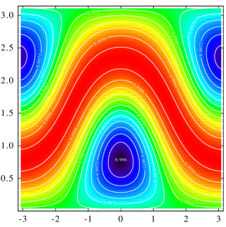
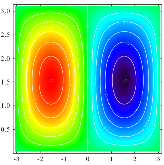
$\vartheta$

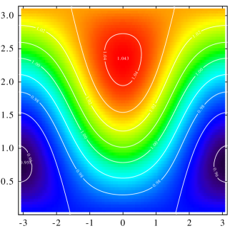
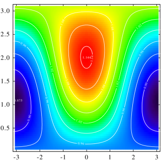
$\phi$                                                                      $\phi$

Figure 15: For $\beta=0.03$ from top left to bottom right: Degree of polarisation $P$ (5.32), deviation $\alpha-\alpha_{0}$ of the major polarisation direction from tangential in degrees (5.43) frequency blueshift factor $\nu_{\mathrm{sc}}/\nu_{\mathrm{in}}$ (5.5) and total intensity amplification per electron relative to the standard intensity $\pi r_{e}^{2}/2\,\bar{L}_{\odot}(R_{\odot}/r)^{2}$. The values refer to a single beam scattered at $\chi=\pi/2$. The angles $\phi$ and $\vartheta$ are the spherical angles of $\boldsymbol{\hat{\beta}}$ such that $\boldsymbol{\hat{\beta}}\parallel\mathbfl{\hat{k}}_{\mathrm{in}}$ for $\vartheta=0$ and $\boldsymbol{\hat{\beta}}\parallel\mathbfl{\hat{k}}_{\mathrm{sc}}$ for $\phi=0,\vartheta=\pi/2$.

We first present the results for a single beam equivalent to a scattering site at $r\rightarrow\infty$. There is just a single incident beam $\mathbfl{\hat{k}}_{\mathrm{in}}$ along the $\mathbfl{\hat{z}}$-direction and the angle $\vartheta$ between $\mathbfl{\hat{\beta}}$ and $\mathbfl{\hat{k}}_{\mathrm{in}}$ is exactly $\psi_{\mathrm{in}}$. For the scattering angle $\chi=\pi/2$ and for an electron at rest the scattered beam has a polarisation degree of $P=1$ (see eq. 3.39), a tilt of the polarisation from the tangential direction of $\alpha-\alpha_{0}=0$, a frequency shift of unity and a radiant intensity per electron of $I_{\mathrm{tot}}=I_{\mathrm{tan}}=r_{e}^{2}/2\;\bar{L}_{\odot}(R_{\odot}/r)^{2}$ (see eq 3.40). We will take the last value as reference $I_{\mathrm{ref}}$ for the intensity amplification presented for the relativistic case.

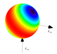
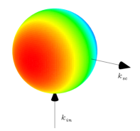
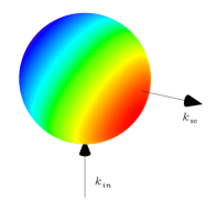
Figure 16: Results of Fig. 15 replotted on a 3D sphere to better illustrate the 3D variation with $\mathbfl{\hat{\beta}}$ in space and their relation to the incident and scattered beam direction. From left to right: Degree of polarisation, deviation of the major polarisation direction from tangential and total intensity amplification per electron. The colour code is the same as in Fig. 15.

On the top left panels of Figs. 15 we show the small deviations from these non-relativistic values for $\beta$=0.03 which is about twice the thermal speed of a coronal electron. The polarisation degree varies between $P=0.996$ and 1 and the polarisation axis is titled away from the tangential direction between $\pm 1.7^{\circ}$. The photon frequency is shifted by up to $\pm$4% and the total intensity is amplified by up to $\pm$11%. All these variations depend on the direction of $\boldsymbol{\hat{\beta}}$. To better illustrate this dependency, we have replotted $P$, $\alpha-\alpha_{0}$ and $I_{\mathrm{tot}}/I_{\mathrm{ref}}$ on a unit sphere in Fig. 16.

From this representation it can be seen that the minimum degree of the polarisation is reached at directions of $\boldsymbol{\hat{\beta}}$ along $\pm(\mathbfl{\hat{k}}_{\mathrm{sc}}+\mathbfl{\hat{k}}_{\mathrm{in}})$. For $\boldsymbol{\hat{\beta}}$ in the plane normal to this axis we have $P=1$. As can be easily checked for electron velocities in the plane $\boldsymbol{\hat{\beta}}{}^{\mathsf{T}}(\mathbfl{\hat{k}}_{\mathrm{sc}}+\mathbfl{\hat{k}}_{\mathrm{in}})=0$ the scattering angle in the electron rest frame is $\chi^{\prime}=\pi/2$. The strongest polarisation tilt occurs for $\boldsymbol{\hat{\beta}}$ pointing normal to the scattering plane. If $\boldsymbol{\hat{\beta}}$ lies in the scattering plane, the aberration planes coincide with the scattering planes in the Sun’s frame and the scattering plane in the electron’s frame is unchanged from the Sun’s frame. The strongest frequency blueshift and intensity amplification occur when $\boldsymbol{\hat{\beta}}$ points to $\mathbfl{\hat{k}}_{\mathrm{sc}}-\mathbfl{\hat{k}}_{\mathrm{in}}$. For this electron velocity direction the scattered photon frequency is upshifted twice because electron sees the incident electron upshifted and the observer sees the electron scattered emission upshifted. The parameters $P$, $\nu_{\mathrm{sc}}/\nu_{\mathrm{in}}$ and $I_{\mathrm{tot}}/I_{\mathrm{ref}}$ vary symmetrically with angle $\phi$, i.e. there is symmetry for $\boldsymbol{\hat{\beta}}$ with respect to the scattering plane in the Sun’s rest frame. The polarisation tilt angle $\alpha-\alpha_{0}$ varies antisymmetrically instead. In general, we find that for this small value of $\beta$ all four beam parameters change sign when $\boldsymbol{\hat{\beta}}$ reverses sign which indicates that they are perturbed only linearly by $\boldsymbol{\beta}$.

$\vartheta$

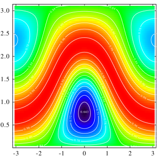
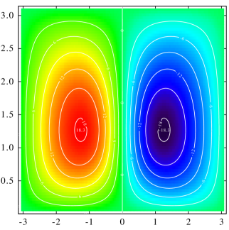
$\vartheta$

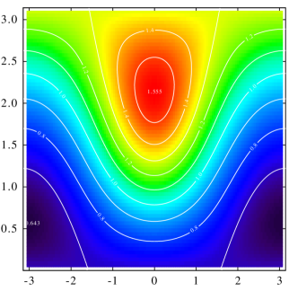
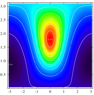
$\phi$                                                                      $\phi$
.

Figure 17: Same as Fig. 15 but for $\beta=0.3$ From top left to bottom right: Degree of polarisation, deviation of the major polarisation direction from tangential in degrees, frequency blueshift factor and total intensity amplification per electron.

$\vartheta$

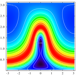
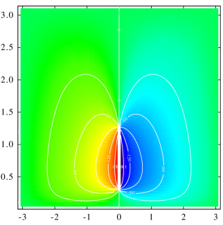
$\vartheta$

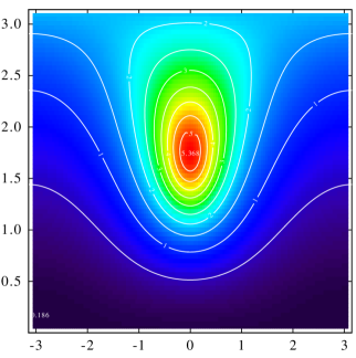
$\phi$                                                                      $\phi$

Figure 18: Same as Fig. 15 but for $\beta=0.8$ From top left to bottom right: Degree of polarisation, deviation of the major polarisation direction from tangential in degrees, frequency blueshift factor and total radiant intensity amplification per electron.

This antisymmetry with respect to $\pm\boldsymbol{\hat{\beta}}$ is lost when $\beta$ is enhanced, only the (anti)symmetry with respect to the scattering plane remains. In Figs. 17 and 18 we show the four beam parameters for $\beta=0.3$ and 0.8, respectively. The minimum degree of the polarisation reached is $P=0.643$ for $\beta=0.3$ and even $P=0$ for $\beta=0.8$. The direction of $\boldsymbol{\hat{\beta}}$ for this minimal $P$ concentrates more and more on the scattering plane with directions in the quadrant between $\mathbfl{\hat{k}}_{\mathrm{in}}$ and $\mathbfl{\hat{k}}_{\mathrm{sc}}$. In the reverse direction the minimum is much less pronounced with $P=0.75$ and 0.18 for $\beta=0.3$ and 0.8, respectively. The surface $P=1$ has its normal inclined closer to $\mathbfl{\hat{k}}_{\mathrm{in}}$ as $\beta$ is enhanced and it is not dissolved despite the relativistic speed of the electron.

The most extreme values of the polarisation tilt angle for $\beta=0.3$ are $\alpha-\alpha_{0}=\pm 18.3^{\circ}$. They are assumed for $\boldsymbol{\hat{\beta}}$ not any more exactly normal to the scattering plane but inclined by 18^∘ towards the quadrant between $\mathbfl{\hat{k}}_{\mathrm{in}}$ and $\mathbfl{\hat{k}}_{\mathrm{sc}}$. For larger $\beta$ this tendency continues so that for $\beta=0.8$ the extreme tilt angles reach $\alpha-\alpha_{0}=\pm 180^{\circ}$ in directions for $\boldsymbol{\hat{\beta}}$ which collapse on the quadrant between $\mathbfl{\hat{k}}_{\mathrm{in}}$ and $\mathbfl{\hat{k}}_{\mathrm{sc}}$. Note that polarisation tilt angles of $\pm 180^{\circ}$ and $0^{\circ}$ are equivalent so that the tilt angle rotates continuously through the tangential direction as $\boldsymbol{\hat{\beta}}$ crosses the scattering plane at the quadrant between $\mathbfl{\hat{k}}_{\mathrm{in}}$ and $\mathbfl{\hat{k}}_{\mathrm{sc}}$.

The frequency shift and the radiant intensity also concentrate their maximum with increasing $\beta$ in the forward direction $\boldsymbol{\hat{\beta}}$ of the electron. This complies with the headlight effect discussed qualitatively above. For $\beta$=0.3, a maximum blueshift factor of 1.55 is obtained when $\boldsymbol{\hat{\beta}}$ points only 122^∘ away from $\mathbfl{\hat{k}}_{\mathrm{in}}$ and 32^∘ from $\mathbfl{\hat{k}}_{\mathrm{sc}}$. In the reverse direction, the factor is 0.643 which corresponds to a red shift of 1/0.643=1.55. For $\beta=0.8$ the maximum blueshift factor is 5.37 reached when $\boldsymbol{\hat{\beta}}$ is almost parallel to $\mathbfl{\hat{k}}_{\mathrm{sc}}$, i.e., when the electron emission is seen with maximum blueshift. Accordingly, the strongest redshift is by factor 0.186=1/5.37 in direction $\boldsymbol{\hat{\beta}}\parallel\mathbfl{\hat{k}}_{\mathrm{in}}$ when the scattering electron sees the incoming photon with the strongest redshift. The maximum radiant intensity is enhanced by a factor 4.30 above the non-relativistic value for $\beta=0.3$ and even by 370 at $\beta=0.8$. This strong amplification in the forward direction of the electron is due to the headlight effect and is formally a consequence of the factor $D^{4}(\mathbfl{\hat{k}}_{\mathrm{sc}},\boldsymbol{\beta})/D^{2}(\mathbfl{\hat{k}}_{\mathrm{in}},\boldsymbol{\beta})$ in (5.23). In forward direction, i.e. for $\psi_{\mathrm{sc}}=0$ and $\psi_{\mathrm{in}}=0$, this alone factor amounts to $\beta(1+\beta)/(1-\beta)^{3}=180$ for $\beta=0.8$.

$\vartheta$

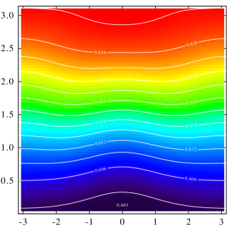
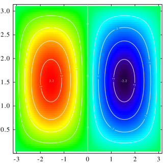
$\vartheta$

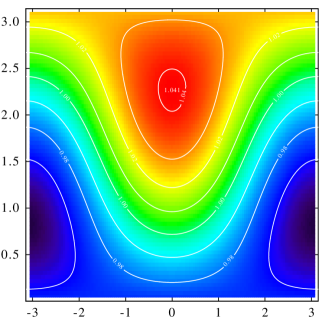
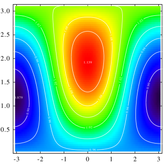
$\phi$                                                                      $\phi$

Figure 19: For $\beta=0.03$ from top left to bottom right: Degree of polarisation $P$ and deviation $\alpha-\alpha_{0}$ of the major polarisation direction from tangential in degrees (5.27), intensity-weighted effective frequency blueshift factor $\nu_{\mathrm{sc}}/\nu_{\mathrm{in}}$ and total radiant intensity amplification for an electron at rest. The values shown refer to a scattering electron at a distance $r=1.50R_{\odot}$ from Sun centre and at a scattering angle $\bar{\chi}=\pi/2$. The angles $\phi$ and $\vartheta$ are the spherical angles of $\boldsymbol{\hat{\beta}}$ as in Fig 15.

$\vartheta$

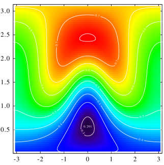
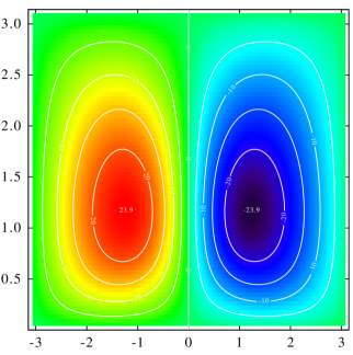
$\vartheta$

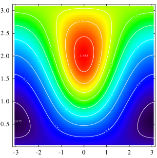
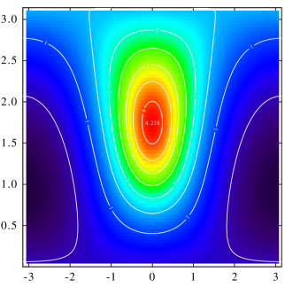
$\phi$                                                                      $\phi$

Figure 20: Same as Fig. 19 but for $\beta=0.3$ From top left to bottom right: Degree of polarisation, deviation of the major polarisation direction from tangential in degrees, frequency blueshift factor and total radiant intensity amplification per electron.

$\vartheta$

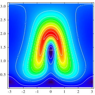
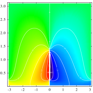
$\vartheta$

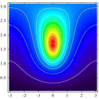
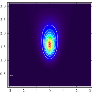
$\phi$                                                                      $\phi$

Figure 21: Same as Fig. 19 but for $\beta=0.8$ From top left to bottom right: Degree of polarisation, deviation of the major polarisation direction from tangential in degrees, frequency blueshift factor and total radiant intensity amplification per electron.

The above results for a single incident beam are applicable to the scattering of Sun light at large distances $r$ when the solid view angle $\Omega(r)$ subtended by the solar disk at the scattering distance $r$ shrinks to a point. For closer distances to the Sun, we have to integrate the directions $\mathbfl{\hat{k}}_{\mathrm{in}}$ in (5.17) over the solid angle cone $\Omega(r)$ of the apparent Sun. The integrand is too involved to allow an analytical integration, a numerical integration is however straight forward. We use Gaussian-Legendre integration for the $\theta$ angle and Simpson in azimuth.

In Figs. 19, 20 and 21 we plot the same parameters as above, now however for the scattering electron at the finite distance $r=1.5R_{\odot}$ and for a mean scattering angle of again $\bar{\chi}=\pi/2$. The difference to the single beam case is the integration of the incident radiation directions $\mathbfl{\hat{k}}_{\mathrm{in}}$ over a finite cone $\Omega$. At $r=1.5R_{\odot}$ the visible solar disk subtends a central cone angle of 41^∘. For an electron at rest, we can derive from (3.37) and (3.38) a polarisation degree $P=0.62214$, a polarisation tilt $\alpha-\alpha_{0}=0$, a frequency shift of unity and a total scattered radiant intensity per electron of $I_{\mathrm{ref}}=I_{\mathrm{tan}}+I_{\mathrm{rad}}=5.4541\;10^{-30}~{}\mathrm{m}^{2}\;L_{\odot}$.

In Fig. 19, we show the results for the same parameters as in Fig. 15 again for $\beta=0.03$ but $r=1.5$ instead $r\rightarrow\infty$. The integration over $\Omega$ has very little effect on the polarisation tilt, the frequency shift and the total intensity. The maximum tilt of the polarisation angle is somewhat intensified to $\pm 2.2^{\circ}$ for an electron velocity direction normal to the mean scattering plane. The strongest modification is found for the degree of polarisation (top left of Fig. 19). It varies between $P=0.603$ and 0.639. The deviation from the standard value for an electron at rest is roughly proportional to $-\cos\vartheta$, i.e., to the radial component of $-\boldsymbol{\hat{\beta}}$. This conforms with Molodensky’s qualitative argument [Molodensky, 1973] mentioned above: the degree of polarisation decreases the faster the electron moves away from the Sun because then the Sun appears bigger in the electron rest frame. An inward moving electron sees a smaller apparent size and consequently a enhanced polarisation.

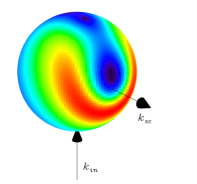
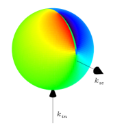
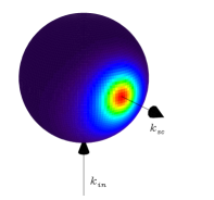
Figure 22: Results of Fig. 21 replotted on a 3D sphere to better illustrate the 3D variation with $\mathbfl{\hat{\beta}}$ in space and their relation to the incident and scattered beam direction. From left to right: Degree of polarisation, deviation of the major polarisation direction from tangential and relative scattered total radiant intensity per electron. The colour code is the same as in Fig. 21.

For higher values of $\beta=0.3$ and 0.8 the results are displayed in Figs. 20 and 21. Again the forward beaming of the scattering electron becomes increasingly important similarly to what we found for the single incident beam. The distribution of the polarisation tilt angle, the frequency shift and the total intensity amplification are similar to Figs. 17 and 18. The exception again is the degree of polarisation and it can again qualitatively be explained by the Molodensky effect. For outward directed $\boldsymbol{\hat{\beta}}$, i.e. $\vartheta>0$, the apparent size of the Sun in the electron rest frame is so much enhanced that $P$ becomes strongly reduced and the scattered radiation is almost unpolarised. In the reverse direction, the Sun’s size appears strongly reduced and the conditions resemble closely the single beam case with a maximum polarisation of almost unity for $\boldsymbol{\hat{\beta}}$ in the scattering plane plane. An electron at $r=1.5$ moving with $\beta=0.8$ away from the Sun sees the cone angle of the solar disk increased from 41^∘ to 98^∘, in opposite direction the apparent solar disk shrinks to 14^∘. In Fig. 22 we have replotted the variation of the polarisation degree, the tilt angle and the total intensity amplification with the electron velocity direction on a 3D sphere.

The frequency shifts shown are always means over the visible solar disk weighted by the respective radiance. However, each incoming beam experiences its individual frequency shift which may well deviate from the average. If the shift is so large that the scattered beam falls out of the frequency band of the observing instrument, it will not be able to contribute to the observation and the observed averages of the angle and degree of polarisation, of frequency shift and total intensity will change because of this omission.

The results described so far refer to only a single electron. In order to derive the full signal observed in a coronagraph pixel, we have to integrate the radiant intensity per electron times the local number of electrons along the line-of-sight as in (3.41). However, since the radiant intensity matrix now also depends on $\boldsymbol{\beta}$ we have also to sum over the electron velocities weighted by the local distribution function $f(\boldsymbol{\beta})$ normalised to $\int f(\boldsymbol{\beta})\,d^{3}\boldsymbol{\beta}=1$. For a polariser oriented along $\mathbfl{\hat{p}}$, the radiant flux per pixel observed at $\mathbfl{r}_{\mathrm{obs}}$ will be

$$\Phi{\hat{p}}(\mathbfl{r}_{\mathrm{obs}})=\frac{A_{\mathrm{pixel}}A_{\mathrm{aperture}}}{f^{2}}\int_{\mathrm{LOS}}\int_{\mathrm{velocity~{}space}}\mspace{-20.0mu}\mathbfl{\hat{p}}^{\mathsf{T}}\mathbfl{I}(\mathbfl{\hat{k}}_{\mathrm{sc}}(\mathbfl{r}),\boldsymbol{\beta})\mathbfl{\hat{p}}\;\;f(\boldsymbol{\beta})\,d^{3}\boldsymbol{\beta}\;N_{e}(\mathbfl{r})d\ell\qquad\text{[W]}$$ (5.44)

where in the integral $\mathbfl{r}(\ell)=\mathbfl{r}_{\mathrm{obs}}-\ell\mathbfl{\hat{k}}_{\mathrm{sc}}$ denotes the scattering site. The conventional result in (3.41) is recovered if $f(\boldsymbol{\beta})$ is confined to non-relativistic velocities. Whether we retain a measurable relativistic effect therefore depends on the number of energetic electrons along the line-of-sight compared to the cold core of the distribution function.

But even if $f(\boldsymbol{\beta})$ has a high energy tail, the velocity integration in (5.44) has consequences. The antisymmetry of the polarisation tilt angle with respect to the $\phi$-angle of $\boldsymbol{\beta}$ cancels the collective tilt of the polarisation axis with respect to $\mathbfl{\hat{p}}_{\mathrm{tan}}$ in the case of an isotropic electron velocity distribution function $f(\boldsymbol{\beta})$. Reversely, the observation of a deviation of the polarisation from the tangential direction could be evidence for a relativistic electron beam.

Figure 23: Degree of polarisation (left), effective frequency shift (centre) and radiant intensity amplification (right) integrated over an isotropic Jüttner distribution with thermal energy $E_{\mathrm{therm}}$. The thermal speed $\beta_{\mathrm{therm}}$ corresponding to $E_{\mathrm{therm}}$ is marked at the top edge of the diagrams. The scattering site is assumed at $r=1.5R_{\odot}$ and the mean scattering angle is $\bar{\chi}=\pi/2$ as in Figs. 19, 20 and 21.

The relativistic effects on the degree of polarisation, on the frequency shift and on the radiant intensity amplification remain even for isotropic distribution functions. In Fig. 23 we show these three parameters if we integrate over a relativistic Jüttner distribution function of various thermal energies. This distribution function is isotropic and the relativistic extension of a Maxwell distribution function. More details are given in the appendix in chapter D.6. The velocity-space integration results in a net depolarisation of the scattered signal. Recall that P=0.622 is the polarisation obtained for non-relativistic electrons at $r=1.5$ and a mean scattering angle $\bar{\chi}=\pi/2$. However the decrease saturates at $P\simeq 0.177$ which we again attribute to the Molodensky effect: for one half of the electron distribution the Sun’s size becomes so huge that these particles scatter practically unpolarised, while for the other half the Sun reduces to a point source contributing a polarisation like in the single beam case in Fig. 15. Both the frequency shift and the intensity amplification not only intensify in the forward direction of the scattered electron as we have seen above but also their spherical average increases strongly with $\beta$. The excess energy of the scattered photon is taken from the kinetic energy of the electron. However, by using the Thomson cross section in the electron rest frame we here neglect the corresponding energy loss for the electron in the scattering process.

6 Discussion and summary

We have reformulated the classical Thomson scattering problem for the corona. The final result is not new, but the new derivation may provide some new understanding of the details of the process. The analytical integrals $A(r)$, $B(r)$, $C(r)$ and $D(r)$ first derived by Schuster [1879] and Minnaert [1930] are not related to Thomson scattering at all but they already arise when the electric field correlation matrix $\mathbfl{Q}_{\mathrm{in}}\propto\;<\!\mathbfl{E}\mathbfl{E}^{\mathsf{T}}\!>$ of the solar incident irradiance at the scattering site is calculated. The subsequent scattering process can be considered essentially as a simple projection of $\mathbfl{Q}_{\mathrm{in}}$ into the direction toward the observer. Our general result (3.35) allows to easily calculate the Thomson scattered radiant intensity per electron for incident radiation from the apparent solar disk for all possible observed polarisation directions. The details of our calculations are included in an extensive appendix. It is therefore entirely transparent how they have to be extended if, e.g., the limb darkening is required to include terms of higher than linear degree in $\cos\zeta$, or the effects of a huge sun spot or a local polarised radiation source on the solar surface are to be determined.

Each point along the observed line-of-sight contributes to the observed signal $N_{e}$ times the local radiant intensity per electron. Due to the simple nature of Thomson scattering, the tangential radiant intensity polarised normal to the mean scattering plane does not depend on the scattering angle. Only the radially polarised radiant intensity $I_{\mathrm{rad}}$ depends on it. It has been argued that the contribution from the Thomson sphere, defined as the surface where the mean scattering is $\bar{\chi}=\pi/2$, will dominate the scattered signal from a given line-of-sight [Vourlidas and Howard, 2006]. The relevance of the Thomson sphere for coronal Thomson scattering has been extensively discussed by Howard and DeForest [2012] and we can only reiterate here their main arguments which are confirmed by our results. The maximum of $I_{\mathrm{tot}}$ and $I_{\mathrm{pol}}$ on the Thomson sphere is not due to peculiarities of the differential Thomson cross section but it is a consequence of the decrease of the entire line-of-sight integrand with distance $r$ from the solar centre. This is due to the decrease of both, the incident solar irradiance and of the scattering electron density with distance $r$. For the total radiant intensity $I_{\mathrm{tot}}$ it is even the reverse, since $I_{\mathrm{rad}}$ almost vanishes on the Thomson sphere it compensates in part the maximum of $I_{\mathrm{tan}}$ along line-of-sight. In this respect the term “Thomson sphere” is misleading.

For large elevation angles $\varepsilon$ from the Sun and an assumed $N_{e}\propto r^{-}2$ dependence the line-of-sight integrand varies with scattering angle $\bar{\chi}$ like $\propto 1-\cos^{4}\bar{\chi}$ for the total and $\propto\sin^{4}\bar{\chi}$ for the tangentially polarised scatter signal (see eqs. 4.14, 4.13 and also [Howard and DeForest, 2012, DeForest et al., 2013]). Therefore the decrease of the line-of-sight integrand off the Thomson sphere is very moderate compared to the gradient of the electron density at the boundaries of streamers, current sheets and CMEs. These objects therefore may well be detectable in coronagraph images even if they occur far off the Thomson sphere. Instructive examples of forward calculations of line-of-sight integrals have, e.g., been produced from MHD simulations of shocks by Xiong et al. [2013a, b].

The classical expression (3.41) of the observed scattered power per pixel has been used in many papers to estimate the column mass of the plasma inside the cone of resolution subtended by a sensor pixel. Using suitable pre-event difference images and summing over all relevant pixels, the total mass of transients were estimated. The unknown variation of the electron density along the respective lines-of-sight in (3.41) was replaced in many of these studies by a $\delta$-distribution in the plane-of-sky. Vourlidas and Howard [2006] and Colaninno and Vourlidas [2009] pointed out that this leads to an underestimate of the CME mass when in reality it propagates at some angle with the plane-of-sky. They suggested to centre the $\delta$-distribution rather at the true propagation angle which can be estimated either from the location of the source region on the solar surface, from a comparison of the observed scattered power in different polarisations or from a triangulation from two different directions as provided by the STEREO mission [Howard et al., 2008]. In chapter 4.2, we show how these mass estimates are modified further if a more realistic finite width of the CME mass distribution along the line-of-sight is taken account of. If the true width is difficult to estimate to sufficient precision, the variation of the line-of-sight integrals over Gaussian density distributions with different widths $\delta\bar{\chi}$ as presented in Figs. 11 and  12 can still be used to guess the error of the mass estimate. From the examples shown in these figures, it could well amount to 10% or more, depending on the viewing geometry.

To demonstrate the versatility of our approach to calculate the Thomson scattered radiant intensity, we have extended it to the case of relativistic electrons. For coronal applications, similar calculations were initiated Molodensky [1973], but he only considers electron velocity vectors $\mathbfl{v}$ in the plane-of-the-sky and treats only a single incident beam. Nikoghossian and Koutchmy [2001, 2002] extended the electron velocity directions and also consider a finite size of the apparent solar disk but they restrict their calculations to the scattered total intensity $I_{\mathrm{tot}}$ and its net frequency shift. We think that our approach is more intuitive and transparent than these previous calculations and it yields the full set of Stokes parameters for the scattered signal. The resulting expressions (5.23) and (5.24) for the scattered radiant intensity per electron is verified by an alternative but more tedious derivation presented in the appendix.

The coronal scattering resembles in many aspects Thomson and inverse Compton scattering processes in astrophysics which have received a growing interest in recent years. An example are relativistic jets escaping from active galactic nuclei which scatter their own synchrotron radiation as well as low energy photons of the cosmic microwave background up to X-ray energies. The polarisation of this X-ray radiation could help to distinguish how much each of the sources contribute [e.g., McNamara et al., 2009].

Thomson scattering is also of considerable interest in fusion plasma devices as a diagnostic tool. In order to interpret the scattered signal the measured response has been calculated by a number of authors [e.g., Hutchinson, 2002, Segre and Zanza, 2000, Beausang and Prunty, 2008]. As is appropriate for laboratory plasmas, the calculations concentrate on monochromatic, linearly polarised incident beams and assume that the electron distribution is an isotropic Maxwellian or Jüttnerian. Since in fusion plasmas the electrons may reach several tens of keV , relativistic effects are observed as a skewed spectral spread with a net blue-shift of the scattered signal and its depolarisation with increasing electron energy.

Whether similar deviations from the non-relativistic standard can be observed in the corona depends critically on the number of relativistic electrons compared to cold electrons with $\beta<10^{-2}$ and on the precision of the observations. For a pixel with resolution of $\Delta\theta=2^{\prime\prime}$ pointing close to the limb so that the maximum electron density along the line-of-sight is $N_{e}=10^{15}\mathrm{m}^{-3}$ we find approximately a total number of electrons scattering into the pixel of

$$N_{e}(200R_{\odot}\Delta\theta)^{2}R_{\odot}=0.4\;10^{-6}R_{\odot}^{3}N_{e}\simeq 10^{35}$$

This is just two orders of magnitude larger than the $10^{33}$ electrons at several keV required to produce an X-ray flare and an associated type III radio burst [Aschwanden et al., 1995]. Locally, the relativistic electrons may represent 10% and more of the total electrons [Krucker et al., 2010, Chen and Petrosian, 2012]. The acceleration of these electrons probably takes place well above the solar surface in above-the-loop-top magnetic x-point configurations [Krucker et al., 2010, Mann and Warmuth, 2011, Carley et al., 2015]. The acceleration sites therefore seem accessible to coronagraph observations and above some large X-ray flares the number of relativistic electrons may be sufficient to yield a detectable signal. Note that the occurrence rate of flares has a power-law dependence on energy [e.g., Li et al., 2012]. More energetic flares occur less often but it seems that the most energetic events observed so far were limited by statistical probability rather than by a fundamental absolute upper energy boundary.

When evaluating the probability of detecting relativistic scattering effects it also has to be kept in mind that a single relativistic electron amplifies the scattered radiation considerably. The scattered radiant intensity strongly increases with $\beta$ not only in their forward direction due to beaming but also on average (see Fig. 23). The intensification with $\beta$ eventually stops if Thomson scattering is no more appropriate in the electron rest frame and has to be replaced by Compton scattering.

Even for an electron energy of 0.03 keV which is just twice their thermal energy in the corona we see small relativistic effects. Deviations from the non-relativistic limit of the polarisation degree are of the order of a few %, and the polarisation angle may be inclined by up to about $2^{\circ}$ away from the tangential direction. Deviations of this order of magnitude may be produced all along the line-of-sight and can be considered as the thermal noise of the corona in these measurable parameters. But observations which can uniquely be attributed to the Thomson scattering of relativistic electrons are still scarce. A net frequency shift in coronal threads above flaring active regions were predicted by Koutchmy and Nikoghossian [2002] and later observed in a few cases as deviations of a scaled colour index from unity which were derived from colour-filtered coronagraph data [Koutchmy and Nikoghossian, 2005].

Unexpectedly large degrees of polarisation have been observed by a number of authors [Koutchmy and Schatten, 1971, Pepin, 1970, Skomorovsky et al., 2012, Qu et al., 2013]. In these cases, the degree of polarisation exceeded the maximum non-relativistic Thomson scatter value expected for the observed elongation at a scattering angle $\bar{\chi}=\pi/2$. As we have seen, an isotropic relativistic electron velocity distribution should lead to a depolarisation of the observed scattering signal. Enhancements of the polarisation degree beyond the non-relativistic $\bar{\chi}=\pi/2$ maximum could be produced by relativistic electron beams with a velocity vector near the scattering plane and a velocity component towards the Sun. Alternatively, contaminations of the scattered white-light signal by coronal ion emission lines could alter the degree of polarisation. Qu et al. [2013] favoured this explanation for large polarisation degrees they observed closely above the limb where non-relativistic Thomson scatter should yield particularly low values for the polarisation degree.

Deviations of the polarisation orientation of the scattered signal from tangential have also been reported only seldomly. This may be due to the fact that a tangential polarisation is often firmly assumed and even used as a premise to separate F and K corona [Koutchmy, 1994] or to eliminate a polarisation bias due to seeing or instrumental effects [Kulijanishvili and Kapanadze, 2005]. Anomalous polarisation directions were reported by [Pepin, 1970, Park et al., 2001, Skomorovsky et al., 2012, Qu et al., 2013] while other studies explicitly found no deviation from tangential polarisation within the measurement error [Koutchmy et al., 1993, Kim et al., 1996, Kulijanishvili and Kapanadze, 2005]. All of these studies were made during lunar eclipses and can at best represent a snapshot of the state of the corona. On the other hand, years of space-borne coronagraph data has been collected in recent years. A systematic scan of the polarisation data from these collections by comparing the angle of polarisation with the heliocentric azimuth angle of every pixel could yield outliers which may be associated with nearby flares. For a few images such a scan was produced from STEREO/SECCHI coronagraph data by [Moran et al., 2006]. However, they assumed the scattered signal to be tangentially polarised and their incentive was to check the polarimetric performance of their instrument rather than to search for true observations of an anomalous polarisation.

Appendix

Appendix A Minnaert’s coefficients

In this appendix we calculate the four integrals (3.6) and (3.16) relevant for the irradiance matrix elements at some distance $r>R_{\odot}$ from the solar centre. We also derive the indefinite integrals required for the case that the limb darkening of the surface radiance $L(\cos\zeta)$ is expressed in a power series of $\cos\zeta$ involving powers higher than $n=1$.

A.1 Integration of the surface radiance

The first step is a variable transformation from the spherical integration angle $\theta$ to $x=(r/R_{\odot})\cos\theta$. Using $\sin\theta_{\mathrm{max}}=R_{\odot}/r$ from (3.2) and (3.3) we find for the transformed lower integration boundary becomes

$$x_{\mathrm{min}}=\frac{r}{R_{\odot}}\cos\theta_{\mathrm{max}}=\frac{r}{R_{\odot}}\sqrt{1-\sin^{2}\theta_{\mathrm{max}}}=\sqrt{(\frac{r}{R_{\odot}})^{2}-1}=\cot\theta_{\mathrm{max}}\quad\text{and}$$

$$\frac{r}{R_{\odot}}=\sin^{-1}\theta_{\mathrm{max}}=\sqrt{1+x^{2}_{\mathrm{min}}}$$ (A.1)

The cosine (3.3) of the local zenith angle of the beam from the solar surface to the scattering site then is

$$\cos\zeta=\sqrt{x^{2}-x^{2}_{\mathrm{min}}}$$

This variable transformation results in four type of integrals which occur in (3.1), (3.6), (3.15) and (3.16)

$$\begin{Bmatrix}I(r)\\ J(r)\end{Bmatrix}=2\pi\int^{1}_{\cos\theta_{\mathrm{max}}}\mspace{-10.0mu}L(\sqrt{x^{2}-x_{\mathrm{min}}^{2}})\begin{Bmatrix}1\\ \cos^{2}\theta\end{Bmatrix}\;d\cos\theta$$

$$\;\stackrel{{\scriptstyle x=(r/R_{\odot})\cos\theta}}{{=}}\;2\pi\frac{R_{\odot}}{r}\int^{\sqrt{1+x^{2}_{\mathrm{min}}}}_{x_{\mathrm{min}}}L(\sqrt{x^{2}-x_{\mathrm{min}}^{2}})\begin{Bmatrix}1\\ x^{2}\end{Bmatrix}\;dx$$ (A.2)

The solar limb darkening of the surface radiance can be represented by the power series $L(\cos\zeta)=\sum_{k=0}^{n}b_{k}\cos^{k}\zeta$ where $\zeta$ is the local zenith angle at the surface. We here follow the previous literature and employ only terms up to $n=1$ and express the limb darkening by $L(\cos\zeta)=(1-u)+u\cos\zeta$. Then (A.2) results in the two integrals $I_{0}$ and $J_{0}$ as coefficients of $1-u$ and two more integrals $I_{1}$ and $J_{1}$ as coefficients of $u$. These integrals can be expressed by elementary functions

$$I_{0}(r)=2\pi\int^{1}_{\cos\theta_{\mathrm{max}}}\mspace{-10.0mu}d\cos\theta=2\pi(1-\cos\theta_{\mathrm{max}})$$ (A.3)

$$J_{0}(r)=2\pi\int^{1}_{\cos\theta_{\mathrm{max}}}\mspace{-10.0mu}\cos^{2}\theta\;d\cos\theta=\frac{2\pi}{3}(1-\cos^{3}\theta_{\mathrm{max}})$$ (A.4)

$$I_{1}(r)=2\pi\int^{1}_{\cos\theta_{\mathrm{max}}}\mspace{-10.0mu}\cos\zeta\;d\cos\theta=2\pi\frac{R_{\odot}}{r}\;\int^{\sqrt{1+x^{2}_{\mathrm{min}}}}_{x_{\mathrm{min}}}\sqrt{x^{2}-x_{\mathrm{min}}^{2}}\;dx$$

$$\stackrel{{\scriptstyle(\ref{I1_app})}}{{=}}2\pi\frac{R_{\odot}}{r}\;\left[\frac{x}{2}\sqrt{x^{2}-x_{\mathrm{min}}^{2}}-\frac{x_{\mathrm{min}}^{2}}{2}\ln(x+\sqrt{x^{2}-x_{\mathrm{min}}^{2}})\right]^{\sqrt{1+x^{2}_{\mathrm{min}}}}_{x_{\mathrm{min}}}$$

$$=2\pi\frac{R_{\odot}}{r}\;\left[\frac{1}{2}\sqrt{1+x^{2}_{\mathrm{min}}}-\frac{x_{\mathrm{min}}^{2}}{2}\ln(\sqrt{1+x^{2}_{\mathrm{min}}}+1)+\frac{x_{\mathrm{min}}^{2}}{2}\ln(x_{\mathrm{min}})\right]$$

$$=\pi\;\left[1-\frac{\cos^{2}\theta_{\mathrm{max}}}{\sin\theta_{\mathrm{max}}}\ln(\frac{1+\sin\theta_{\mathrm{max}}}{\cos\theta_{\mathrm{max}}})\right]$$ (A.5)

$$J_{1}(r)=\pi\int^{1}_{\cos\theta_{\mathrm{max}}}\mspace{-10.0mu}\cos\zeta\cos^{2}\theta\;d\cos\theta=2\pi(\frac{R_{\odot}}{r})^{3}\;\int^{\sqrt{1+x^{2}_{\mathrm{min}}}}_{x_{\mathrm{min}}}\sqrt{x^{2}-x_{\mathrm{min}}^{2}}\,x^{2}\;dx$$

$$\stackrel{{\scriptstyle(\ref{J1_app})}}{{=}}2\pi(\frac{R_{\odot}}{r})^{3}\;\left[\frac{x}{4}\sqrt{x^{2}-x_{\mathrm{min}}^{2}}^{3}+\frac{xx^{2}_{\mathrm{min}}}{8}\sqrt{x^{2}-x_{\mathrm{min}}^{2}}\right.\hskip 60.00009pt$$

$$\hskip 130.0002pt\left.-\frac{x_{\mathrm{min}}^{4}}{8}\ln(x+\sqrt{x^{2}-x_{\mathrm{min}}^{2}})\right]^{\sqrt{1+x^{2}_{\mathrm{min}}}}_{x_{\mathrm{min}}}$$

$$=2\pi(\frac{R_{\odot}}{r})^{3}\;\left[\frac{1}{4}\sqrt{1+x^{2}_{\mathrm{min}}}+\frac{1}{8}x^{2}_{\mathrm{min}}\sqrt{1+x^{2}_{\mathrm{min}}}\right.\hskip 60.00009pt$$

$$\hskip 60.00009pt\left.-\frac{x_{\mathrm{min}}^{4}}{8}\big{(}\ln(\sqrt{1+x^{2}_{\mathrm{min}}}+1)-\ln x_{\mathrm{min}}\big{)}\right]$$

$$=2\pi(\frac{R_{\odot}}{r})^{2}\;\left[\frac{1}{4}+\frac{1}{8}\cot^{2}\theta_{\mathrm{max}}-\frac{\cos^{4}\theta_{\mathrm{max}}}{8\sin^{3}\theta_{\mathrm{max}}}\ln\frac{1+\sin^{-1}\theta_{\mathrm{max}}}{\cot\theta_{\mathrm{max}}}\right]$$

$$=2\pi\;\left[\frac{1}{4}\sin^{2}\theta_{\mathrm{max}}+\frac{1}{8}\cos^{2}\theta_{\mathrm{max}}-\frac{\cos^{4}\theta_{\mathrm{max}}}{8\sin\theta_{\mathrm{max}}}\ln\frac{1+\sin\theta_{\mathrm{max}}}{\cos\theta_{\mathrm{max}}}\right]$$

$$=\frac{\pi}{2}\;\left[1-\frac{1}{2}\cos^{2}\theta_{\mathrm{max}}-\frac{\cos^{4}\theta_{\mathrm{max}}}{2\sin\theta_{\mathrm{max}}}\ln\frac{1+\sin\theta_{\mathrm{max}}}{\cos\theta_{\mathrm{max}}}\right]$$

$$=\frac{\pi}{2}\;\left[1-\frac{\cos^{2}\theta_{\mathrm{max}}}{2}(1+\frac{\cos^{2}\theta_{\mathrm{max}}}{\sin\theta_{\mathrm{max}}}\ln\frac{1+\sin\theta_{\mathrm{max}}}{\cos\theta_{\mathrm{max}}})\right]$$ (A.6)

The indefinite integrals required above are derived in the subsequent chapter A.2 where we use the abbreviations $a=x_{\mathrm{min}}$, $u=\sqrt{x^{2}-a^{2}}$ and $w=\ln(x+u)$ [see also Gradshteyn and Ryzhik, 1980, 2.271.3 and 2.272.2]. The integral $I_{0}$ corresponds to the total irradiance of a Lambert sphere with unit radiance. $I_{1}$ covers the corresponding linear term in the series expansion of $L$ in $\cos\zeta$. The integrals $J_{0}$ and $J_{1}$ are needed for the expansion of the irradiance to a matrix. In the following chapter A.2 we also derive a recursion for the indefinite integrals $I_{n}$ and $J_{n}$ required for degrees higher than $n=1$.

The expressions commonly used are the following combinations first introduced by [Minnaert, 1930] and later popularised by [Billings, 1966]

$$C=\frac{1}{2\pi}(J_{0}+I_{0})=\frac{1-\cos^{3}\theta_{\mathrm{max}}}{3}+1-\cos\theta_{\mathrm{max}}\hskip 40.00006pt$$

$$\hskip 25.00003pt=\frac{4}{3}-\cos\theta_{\mathrm{max}}-\frac{1}{3}\cos^{3}\theta_{\mathrm{max}}$$ (A.7)

$$A=\frac{1}{2\pi}(3J_{0}-I_{0})=1-\cos^{3}\theta_{\mathrm{max}}-1+\cos\theta_{\mathrm{max}}\hskip 80.00012pt$$

$$\hskip 65.00009pt=\cos\theta_{\mathrm{max}}(1-\cos^{2}\theta_{\mathrm{max}})=\cos\theta_{\mathrm{max}}\sin^{2}\theta_{\mathrm{max}}$$ (A.8)

$$F=\frac{\cos^{2}\theta_{\mathrm{max}}}{\sin\theta_{\mathrm{max}}}\ln\frac{1+\sin\theta_{\mathrm{max}}}{\cos\theta_{\mathrm{max}}}\hskip 45.00006pt$$

$$D=\frac{1}{2\pi}(J_{1}+I_{1})=\frac{1}{2}\left[\frac{1}{2}-\frac{1}{4}\cos^{2}\theta_{\mathrm{max}}-\frac{1}{4}\cos^{2}\theta_{\mathrm{max}}F+1-F\right]$$ (A.9)

$$=\frac{1}{8}\;\left[6-\cos^{2}\theta_{\mathrm{max}}-(4+\cos^{2}\theta_{\mathrm{max}})F\right]$$

$$=\frac{1}{8}\;\left[5+\sin^{2}\theta_{\mathrm{max}}-(5-\sin^{2}\theta_{\mathrm{max}})F\right]$$

$$B=\frac{1}{2\pi}(3J_{1}-I_{1})=\frac{1}{2}\left[\frac{3}{2}-\frac{3}{4}\cos^{2}\theta_{\mathrm{max}}(1+F)-1+F\right]$$

$$=\frac{1}{8}\left[2-3\cos^{2}\theta_{\mathrm{max}}+(4-3\cos^{2}\theta_{\mathrm{max}})F\right]$$

$$=-\frac{1}{8}\left[1-3\sin^{2}\theta_{\mathrm{max}}-(1+3\sin^{2}\theta_{\mathrm{max}})F\right]$$ (A.10)

A.2 Indefinite integrals for $I_{1}$, $J_{1}$ and for further expansion terms of the surface radiance $L(\cos\zeta)$

We here solve the indefinite integrals needed in the previous chapter A.1. In the calculations of Minnaert [1930] and in the main text, only the first two terms in an expansion of the solar radiance $L$ in powers $\cos\zeta$ up to linear term are taken account of. Expansion up to the 5${}^{\text{th}}$ power have been determined by measurements [e.g., Neckel and Labs, 1994, Neckel, 1996]. If these were to be included in the calculation of the scattered radiant intensity per electron, indefinite integrals of the type $I_{m}=\int u^{m}\,dx$ and $J_{m}=\int u^{m}x^{2}\,dx$ are required. We will use the following abbreviations

$$u(x)=\sqrt{x^{2}-a^{2}},\qquad u^{\prime}=\frac{x}{u}$$

$$w(x)=\ln(x+u),\qquad w^{\prime}=\frac{1+u^{\prime}}{x+u}=\frac{1}{x}$$

A transformation of the integration variable $x$ yields

$$\int^{X}\frac{1}{u}\,dx\;\stackrel{{\scriptstyle x=a\cosh z}}{{=}}\;\int^{\mathrm{arcosh}(X/a)}\frac{1}{\sinh z}\sinh zdz$$

$$=\int^{\mathrm{arcosh}(X/a)}dz=\mathrm{arcosh}\frac{X}{a}=\ln(X+u(X))-\ln(a)$$

$$\text{where we used}\qquad dx=a\frac{d\cosh z}{dz}\;dz=a\sinh z\;dz$$

$$\text{and}\quad u^{2}=x^{2}-a^{2}=a^{2}(\cosh^{2}z-1)=a^{2}\sinh^{2}z.$$

$$\text{In short}\qquad\int\frac{1}{u}\,dx=w+\mathrm{const}$$ (A.11)

Next we define more generally the indefinite integrals (omitting $\mathrm{const}$ from now on)

$$V_{n}=\int x^{2n}u\,dx,\qquad W_{n}=\int\frac{x^{2n}}{u}\,dx\qquad\text{where from (\ref{int1/u})}\quad W_{0}=w$$

The integrals are related by the recurrence relations

$$W_{n}=\int\frac{x^{2n}}{u}\,dx=\int(\frac{x^{2n-2}(x^{2}-a^{2})}{u}+a^{2}\frac{x^{2n-2}}{u})\,dx=\int(x^{2n-2}u+a^{2}\int\frac{x^{2n-2}}{u})\,dx$$

$$=V_{n-1}+a^{2}W_{n-1}$$ (A.12)

$$\text{and}\qquad(2n+1)V_{n}=(2n+1)\int x^{2n}u\,dx=\int(x^{2n+1})^{\prime}u\,dx=x^{2n+1}u-\int\frac{x^{2n+2}}{u}\,dx$$

$$=x^{2n+1}u-W_{n+1}=x^{2n+1}u-V_{n}-a^{2}W_{n}\quad\text{or}$$

$$V_{n}=\frac{1}{2n+2}(x^{2n+1}u-a^{2}W_{n})$$ (A.13)

In case of a linear expansion of $L(\cos\zeta)$ we only need the indefinite integrals $V_{0}$ for $I_{1}$ and $V_{1}$ for $J_{1}$. By recurrence of (A.12) and (A.13) we obtain successively

$$W_{0}=w,\qquad V_{0}=\frac{1}{2}(xu-a^{2}w)$$

$$W_{1}=\frac{1}{2}(xu-a^{2}w)+a^{2}w=\frac{1}{2}(xu+a^{2}w)$$

$$V_{1}=\frac{1}{4}(x^{3}u-\frac{a^{2}}{2}(xu+a^{2}w))=(\frac{x^{2}}{4}-\frac{a^{2}}{8})xu-\frac{a^{4}}{8}w$$

$$W_{2}=(\frac{x^{2}}{4}-\frac{a^{2}}{8})xu-\frac{a^{2}}{8}w+\frac{a^{2}}{2}(xu+a^{2}w)=(\frac{x^{2}}{4}+\frac{3a^{2}}{8})xu+\frac{3a^{4}}{8}w$$

$$V_{2}=\frac{1}{6}(x^{5}u-a^{2}(\frac{x^{2}}{4}+\frac{3a^{2}}{8})xu-\frac{3a^{6}}{8}w)=(\frac{x^{4}}{6}-\frac{a^{2}x^{2}}{24}-\frac{3a^{4}}{48})xu-\frac{3a^{6}}{48}w$$

$$\dots$$

More can be derived in the same way. From the web side integrals.wolfram.com

$$V_{3}=\frac{x}{384}(48x^{6}-8a^{2}x^{4}-10a^{4}x^{2}-15a^{6})u-\frac{15a^{8}}{384}w$$

$$V_{4}=\frac{x}{3840}(384x^{8}-48a^{2}x^{6}-56a^{4}x^{4}-70a^{6}x^{2}-105a^{8})u-\frac{105a^{8}}{3840}w$$

$$V_{n}=\frac{x^{2n+1}u}{2n+1}\;\frac{{}_{2}F_{1}(-\frac{1}{2},n+\frac{1}{2},n+\frac{3}{2},\frac{x^{2}}{a^{2}})}{\sqrt{1-\frac{x^{2}}{a^{2}}}}$$

where

$${}_{2}F_{1}(a,b,c,x)=1+\frac{ab}{c}x+\frac{a(a+1)b(b+1)}{2c(c+1)}x^{2}+\frac{a(a+1)(a+2)b(b+1)(b+2)}{2c(c+1)(c+2)}x^{3}+\dots$$

is the hypergeometric function which reduces to a polynomial if $a$ or $b$ is a negative integer. In our case it must be an infinite series because $u$ and $w$ cannot be expressed by a finite polynomial.

The final step is

$$I_{m}=\int u^{m}\,dx=\int(x^{2}-a^{2})^{m/2}\,dx=\begin{cases}\sum\limits_{i=0}^{m/2}\begin{pmatrix}m/2\\ i\end{pmatrix}(-a^{2})^{i-m/2}\int x^{2i}\,dx\\ \sum\limits_{i=0}^{(m-1)/2}\begin{pmatrix}(m-1)/2\\ i\end{pmatrix}(-a^{2})^{i-(m-1)/2}\int x^{2i}u\,dx\end{cases}$$

$$=\begin{cases}\sum\limits_{i=0}^{m/2}\begin{pmatrix}m/2\\ i\end{pmatrix}\displaystyle(-a^{2})^{i-m/2}\frac{x^{2i+1}}{2i+1}&\text{if $m$ even}\\ \sum\limits_{i=0}^{(m-1)/2}\begin{pmatrix}(m-1)/2\\ i\end{pmatrix}(-a^{2})^{i-(m-1)/2}V_{i}&\text{if $m$ odd}\\ \end{cases}$$

$$J_{m}=\int x^{2}u^{m}\,dx=\int x^{2}(x^{2}-a^{2})^{m/2}\,dx=\begin{cases}\sum\limits_{i=0}^{m/2}\begin{pmatrix}m/2\\ i\end{pmatrix}(-a^{2})^{i-m/2}\int x^{2i+2}\,dx\\ \sum\limits_{i=0}^{(m-1)/2}\begin{pmatrix}(m-1)/2\\ i\end{pmatrix}(-a^{2})^{i-(m-1)/2}\int x^{2i+2}u\,dx\end{cases}$$

$$=\begin{cases}\sum\limits_{i=0}^{m/2}\begin{pmatrix}m/2\\ i\end{pmatrix}\displaystyle(-a^{2})^{i-m/2}\frac{x^{2i+3}}{2i+3}&\text{if $m$ even}\\ \sum\limits_{i=0}^{(m-1)/2}\begin{pmatrix}(m-1)/2\\ i\end{pmatrix}(-a^{2})^{i-(m-1)/2}V_{i+1}&\text{if $m$ odd}\\ \end{cases}$$

For the lowest powers we can write down the expressions explicitely

$$I_{1}=V_{0}=\int u\,dx=\frac{1}{2}xu-\frac{a^{2}}{2}w$$ (A.14)

$$I_{2}=\int u^{2}\,dx=\int(x^{2}-a^{2})\,dx=\frac{x^{3}}{3}-a^{2}x$$

$$I_{3}=\int u^{3}\,dx=V_{1}-a^{2}V_{0}=\frac{1}{4}(x^{2}-\frac{5a^{2}}{2})xu+\frac{3}{8}a^{4}w$$

$$I_{4}=\int u^{4}\,dx=\int(x^{4}-2a^{2}x^{2}+a^{4})\,dx=\frac{1}{5}x^{5}-\frac{2}{3}a^{2}x^{3}+a^{4}x$$

$$I_{5}=\int u^{5}\,dx=V_{2}-2a^{2}V_{1}+V_{0}=\frac{1}{48}(8x^{4}-26a^{2}x^{2}+33a^{4})xu-\frac{15}{48}a^{6}w$$

$$\dots$$

$$J_{1}=\int x^{2}u\,dx=V_{1}=\frac{1}{8}(2x^{2}-a^{2})xu-\frac{1}{8}a^{4}w$$ (A.15)

$$J_{2}=\int x^{2}u^{2}\,dx=\int(x^{4}-a^{2}x^{2})\,dx=x^{3}(\frac{1}{5}x^{2}-\frac{1}{3}a^{2})$$

$$J_{3}=\int x^{2}u^{3}\,dx=V_{2}-a^{2}V_{1}=\frac{1}{48}(8x^{4}-14a^{2}x^{2}+3a^{4})xu+\frac{3}{48}a^{6}w$$

$$J_{4}=\int x^{2}u^{4}\,dx=\int(x^{6}-2a^{2}x^{4}+a^{4}x^{2})\,dx=x^{3}(\frac{1}{7}x^{4}-\frac{2}{5}a^{2}x^{2}+\frac{1}{3}a^{4})$$

$$J_{5}=\int x^{2}u^{5}\,dx=V_{3}-2a^{2}V_{2}+a^{4}V_{1}=\frac{1}{384}(48x^{6}-136a^{2}x^{4}+118a^{4}x^{2}-15a^{6})xu-\frac{15}{384}a^{8}w$$

$$\dots$$

From the web side integrals.wolfram.com the general expressions are given as

$$I_{m}=\int u^{m}\,dx=xu^{m}\;\frac{{}_{2}F_{1}(\frac{1}{2},-m,\frac{3}{2},\frac{x^{2}}{a^{2}})}{(1-\frac{x^{2}}{a^{2}})^{m}}$$

$$J_{m}=\int x^{2}u^{m}\,dx=\frac{1}{3}x^{3}u^{m}\;\frac{{}_{2}F_{1}(\frac{3}{2},-\frac{m}{2},\frac{5}{2},\frac{x^{2}}{a^{2}})}{(1-\frac{x^{2}}{a^{2}})^{m/2}}$$

where ${}_{2}F_{1}$ is as above the hypergeometric function.

A.3 Connections with van de Hulst’s coefficients

In the end there are just the two scattered radiant intensities per electron $I_{\mathrm{tan}}$ and $I_{\mathrm{rad}}$ or equivalently, their polarised and total combinations, which are relevant. Thus the four coefficients $A$, $B$, $C$ and $D$ of Minnaert could for our purposes also be reduced to only two. Van de Hulst [1950] introduced two new coefficients $\mathcal{A}$ and $\mathcal{B}$ which do the job, however, they depend besides on $r$ also on $u$. They are used also in other papers [e.g., Saito et al., 1970]. Unfortunately, Van de Hulst’s naming convention allows them to be mixed up with Minnaert’s $A$ and $B$. They are directly related to the integrals (A.3) to (A.6) by [Van de Hulst, 1950, eqs. 11 and 12.]

$$2\mathcal{A}+\mathcal{B}=\frac{(1-u)I_{0}+uI_{1}}{\pi(1-u/3)}=\frac{(1-u)(3C-A)+u(3D-B)}{2(1-u/3)}$$

$$2\mathcal{A}-\mathcal{B}=\frac{(1-u)J_{0}+uJ_{1}}{\pi(1-u/3)}=\frac{(1-u)(A+C)-u(D+B)}{2(1-u/3)}$$

$$\text{or}\quad\mathcal{A}=\frac{(1-u)C+uD}{1-u/3},\quad\mathcal{B}=\frac{(1-u)(C-A)+u(D-B)}{1-u/3}$$ (A.16)

The numerator $1-u/3$ is necessary because our coefficients are normalised to the radiance $L_{\odot}$ at solar centre while $\mathcal{A}$ and $\mathcal{B}$ are normalised to the mean radiance

$$\frac{I_{\mathrm{in}}(r)}{\pi}(\frac{r}{R_{\odot}})^{2}\xrightarrow{r\rightarrow\infty}\bar{L}_{\odot}=(1-u/3)\,L_{\odot}$$

of the solar disk, see (3.8). If we compare (A.16) with (3.19), we see that the irradiance matrix elements $Q_{\mathrm{in,xx}}$ and $Q_{\mathrm{in,zz}}$ are proportional to $\mathcal{A}$ and $\mathcal{B}$, respectively.

A.4 Limit $r\rightarrow\infty$

We here derive the asymptotic series expansions of Minnaert’s coefficients to be used for large $r$ because the exact expressions are numerically unstable in this limit. This can be seen from the fact that some of the terms have to be expanded to fifth order to retain the two leading terms of the series expansion in $\theta_{\mathrm{max}}$. These limiting formulae should preferably be used for large $r$ in the numerical evaluation of the coefficients. A similar expansion for the the Van de Hulst coefficients $\mathcal{A}$ and $\mathcal{B}$ can be found in [Saito et al., 1970]. The limit $r\rightarrow\infty$ implies $\theta_{\mathrm{max}}\rightarrow\frac{R_{\odot}}{r}$ We first give the expansions of some subterms and then compose the final expressions from them.

$$\cos^{2}\theta_{\mathrm{max}}=1-\theta^{2}_{\mathrm{max}}+({\textstyle\frac{2}{24}}+{\textstyle\!\frac{1}{4}})\theta^{4}_{\mathrm{max}}=1-\theta^{2}_{\mathrm{max}}+{\textstyle\!\frac{1}{3}}\theta^{4}_{\mathrm{max}}$$

$$\sin^{-1}\theta_{\mathrm{max}}=\theta^{-1}_{\mathrm{max}}(1-{\textstyle\!\frac{1}{6}}\theta^{2}_{\mathrm{max}}+{\textstyle\frac{1}{120}}\theta^{4}_{\mathrm{max}})^{-1}=\theta^{-1}_{\mathrm{max}}(1+{\textstyle\!\frac{1}{6}}\theta^{2}_{\mathrm{max}}+({\textstyle\frac{1}{36}}-{\textstyle\frac{1}{120}})\theta^{4}_{\mathrm{max}})$$

$$=\theta^{-1}_{\mathrm{max}}(1+{\textstyle\!\frac{1}{6}}\theta^{2}_{\mathrm{max}}+{\textstyle\frac{7}{360}}\theta^{4}_{\mathrm{max}})$$

$$\frac{1+\sin\theta_{\mathrm{max}}}{\cos\theta_{\mathrm{max}}}=\frac{1+\theta_{\mathrm{max}}-{\textstyle\!\frac{1}{6}}\theta^{3}_{\mathrm{max}}+{\textstyle\frac{1}{120}}\theta^{5}_{\mathrm{max}}}{1-{\textstyle\!\frac{1}{2}}\theta^{2}_{\mathrm{max}}+{\textstyle\frac{1}{24}}\theta^{4}_{\mathrm{max}}}$$

$$=(1+\theta_{\mathrm{max}}-{\textstyle\!\frac{1}{6}}\theta^{3}_{\mathrm{max}}+{\textstyle\frac{1}{120}}\theta^{5}_{\mathrm{max}})(1+{\textstyle\!\frac{1}{2}}\theta^{2}_{\mathrm{max}}+({\textstyle\!\frac{1}{4}}-{\textstyle\frac{1}{24}})\theta^{4}_{\mathrm{max}})$$

$$=(1+\theta_{\mathrm{max}}-{\textstyle\!\frac{1}{6}}\theta^{3}_{\mathrm{max}}+{\textstyle\frac{1}{120}}\theta^{5}_{\mathrm{max}})(1+{\textstyle\!\frac{1}{2}}\theta^{2}_{\mathrm{max}}+{\textstyle\frac{5}{24}}\theta^{4}_{\mathrm{max}})$$

$$=1+\theta_{\mathrm{max}}+{\textstyle\!\frac{1}{2}}\theta^{2}_{\mathrm{max}}+({\textstyle\!\frac{1}{2}}-{\textstyle\!\frac{1}{6}})\theta^{3}_{\mathrm{max}}+{\textstyle\frac{5}{24}}\theta^{4}_{\mathrm{max}}+({\textstyle\frac{1}{120}}-{\textstyle\frac{1}{12}}+{\textstyle\frac{5}{24}})\theta^{5}_{\mathrm{max}}$$

$$=1+\theta_{\mathrm{max}}+{\textstyle\!\frac{1}{2}}\theta^{2}_{\mathrm{max}}+{\textstyle\!\frac{1}{3}}\theta^{3}_{\mathrm{max}}+{\textstyle\frac{5}{24}}\theta^{4}_{\mathrm{max}}+{\textstyle\frac{4}{30}}\theta^{5}_{\mathrm{max}}$$

$$\ln(\frac{1+\sin\theta_{\mathrm{max}}}{\cos\theta_{\mathrm{max}}})=\ln(1+\theta_{\mathrm{max}}+{\textstyle\!\frac{1}{2}}\theta^{2}_{\mathrm{max}}+{\textstyle\!\frac{1}{3}}\theta^{3}_{\mathrm{max}}+{\textstyle\frac{5}{24}}\theta^{4}_{\mathrm{max}}+{\textstyle\frac{4}{30}}\theta^{5}_{\mathrm{max}})$$

$$=\theta_{\mathrm{max}}+({\textstyle\!\frac{1}{2}}-{\textstyle\!\frac{1}{2}})\theta^{2}_{\mathrm{max}}+({\textstyle\!\frac{1}{3}}-{\textstyle\!\frac{1}{2}}+{\textstyle\!\frac{1}{3}})\theta^{3}_{\mathrm{max}}+({\textstyle\frac{5}{24}}-{\textstyle\!\frac{1}{3}}-{\textstyle\frac{1}{8}}+{\textstyle\!\frac{1}{2}}-{\textstyle\!\frac{1}{4}})\theta^{4}_{\mathrm{max}}$$

$$+({\textstyle\frac{4}{30}}-{\textstyle\frac{5}{24}}-{\textstyle\!\frac{1}{6}}+{\textstyle\!\frac{1}{3}}+{\textstyle\!\frac{1}{4}}-{\textstyle\!\frac{1}{2}}+{\textstyle\!\frac{1}{5}})\theta^{5}_{\mathrm{max}}=\theta_{\mathrm{max}}+{\textstyle\!\frac{1}{6}}\theta^{3}_{\mathrm{max}}+{\textstyle\frac{1}{24}}\theta^{5}_{\mathrm{max}}$$

$$\frac{1}{\sin\theta_{\mathrm{max}}}\ln(\frac{1+\sin\theta_{\mathrm{max}}}{\cos\theta_{\mathrm{max}}})=(1+{\textstyle\!\frac{1}{6}}\theta^{2}_{\mathrm{max}}+{\textstyle\frac{7}{360}}\theta^{4}_{\mathrm{max}})\frac{1}{\theta_{\mathrm{max}}}(\theta_{\mathrm{max}}+{\textstyle\!\frac{1}{6}}\theta^{3}_{\mathrm{max}}+{\textstyle\frac{1}{24}}\theta^{5}_{\mathrm{max}})$$

$$=(1+{\textstyle\!\frac{1}{6}}\theta^{2}_{\mathrm{max}}+{\textstyle\frac{7}{360}}\theta^{4}_{\mathrm{max}})(1+{\textstyle\!\frac{1}{6}}\theta^{2}_{\mathrm{max}}+{\textstyle\frac{1}{24}}\theta^{4}_{\mathrm{max}})$$

$$=1+{\textstyle\frac{2}{6}}\theta^{2}_{\mathrm{max}}+({\textstyle\frac{1}{24}}+{\textstyle\frac{1}{36}}+{\textstyle\frac{7}{360}})\theta^{4}_{\mathrm{max}}=1+{\textstyle\frac{1}{3}}\theta^{2}_{\mathrm{max}}+{\textstyle\frac{8}{90}}\theta^{4}_{\mathrm{max}}$$

$$\frac{\cos^{2}\theta_{\mathrm{max}}}{\sin\theta_{\mathrm{max}}}\ln(\frac{1+\sin\theta_{\mathrm{max}}}{\cos\theta_{\mathrm{max}}})=(1-\theta^{2}_{\mathrm{max}}+{\textstyle\!\frac{1}{3}}\theta^{4}_{\mathrm{max}})(1+{\textstyle\frac{1}{3}}\theta^{2}_{\mathrm{max}}+{\textstyle\frac{8}{90}}\theta^{4}_{\mathrm{max}})$$

$$=(1-(1-{\textstyle\!\frac{1}{3}})\theta^{2}_{\mathrm{max}}+({\textstyle\!\frac{1}{3}}+{\textstyle\frac{8}{90}}-{\textstyle\!\frac{1}{3}})\theta^{4}_{\mathrm{max}})=1-{\textstyle\frac{2}{3}}\theta^{2}_{\mathrm{max}}+{\textstyle\frac{4}{45}}\theta^{4}_{\mathrm{max}}$$

Using the above expansions for $r\rightarrow\infty$ and $\theta_{\mathrm{max}}\rightarrow\frac{R_{\odot}}{r}$ we have the following limiting relations

$$I_{0}(r)=2\pi(1-\cos\theta_{\mathrm{max}})\xrightarrow{r\rightarrow\infty}I_{0}^{\infty}=\pi(\theta_{\mathrm{max}}^{2}-{\textstyle\frac{1}{12}}\theta_{\mathrm{max}}^{4})$$ (A.17)

$$J_{0}(r)=\frac{2\pi}{3}(1-\cos^{3}\theta_{\mathrm{max}})\xrightarrow{r\rightarrow\infty}J_{0}^{\infty}=\frac{2\pi}{3}(1-(1-{\textstyle\frac{3}{2}}\theta^{2}_{\mathrm{max}}+{\textstyle\frac{7}{8}}\theta^{4}_{\mathrm{max}}))$$

$$=\pi(\theta^{2}_{\mathrm{max}}-{\textstyle\frac{7}{12}}\theta^{4}_{\mathrm{max}})$$ (A.18)

$$I_{1}(r)=\pi\left[1-\frac{\cos^{2}\theta_{\mathrm{max}}}{\sin\theta_{\mathrm{max}}}\ln(\frac{1+\sin\theta_{\mathrm{max}}}{\cos\theta_{\mathrm{max}}})\right]\xrightarrow{r\rightarrow\infty}$$

$$I_{1}^{\infty}=\pi\left[1-(1-{\textstyle\frac{2}{3}}\theta^{2}_{\mathrm{max}}+{\textstyle\frac{4}{45}}\theta^{4}_{\mathrm{max}})\right]$$

$$=\pi({\textstyle\frac{2}{3}}\theta^{2}_{\mathrm{max}}-{\textstyle\frac{4}{45}}\theta^{4}_{\mathrm{max}})$$ (A.19)

$$J_{1}(r)=\frac{\pi}{2}\left[1-\frac{1}{2}\cos^{2}\theta_{\mathrm{max}}(1+\frac{\cos^{2}\theta_{\mathrm{max}}}{\sin\theta_{\mathrm{max}}}\ln\frac{1+\sin\theta_{\mathrm{max}}}{\cos\theta_{\mathrm{max}}})\right]\xrightarrow{r\rightarrow\infty}$$

$$J_{1}^{\infty}=\frac{\pi}{2}\left[1-{\textstyle\!\frac{1}{2}}(1-\theta^{2}_{\mathrm{max}}+{\textstyle\!\frac{1}{3}}\theta^{4}_{\mathrm{max}})(2-{\textstyle\frac{2}{3}}\theta^{2}_{\mathrm{max}}+{\textstyle\frac{4}{45}}\theta^{4}_{\mathrm{max}})\right]$$

$$=\frac{\pi}{2}\left[1-(1-\theta^{2}_{\mathrm{max}}+{\textstyle\!\frac{1}{3}}\theta^{4}_{\mathrm{max}})(1-{\textstyle\frac{1}{3}}\theta^{2}_{\mathrm{max}}+{\textstyle\frac{2}{45}}\theta^{4}_{\mathrm{max}})\right]$$

$$=\frac{\pi}{2}\left[1-(1-(1+{\textstyle\!\frac{1}{3}})\theta^{2}_{\mathrm{max}}+({\textstyle\!\frac{1}{3}}+{\textstyle\frac{2}{45}}+{\textstyle\!\frac{1}{3}})\theta^{4}_{\mathrm{max}})\right]$$

$$=\frac{\pi}{2}({\textstyle\frac{4}{3}}\theta^{2}_{\mathrm{max}}-{\textstyle\frac{32}{45}}\theta^{4}_{\mathrm{max}})=\pi({\textstyle\frac{2}{3}}\theta^{2}_{\mathrm{max}}-{\textstyle\frac{16}{45}}\theta^{4}_{\mathrm{max}})$$ (A.20)

We see that $I_{0}$ and $J_{0}$ and $I_{1}$ and $J_{1}$ have pairwise the same leading term. For large $r$ we therefore find $J_{0}\rightarrow I_{0}$ and $J_{1}\rightarrow I_{1}$. This could have been expected because then $\theta$ is bounded close to zero and $\cos^{2}\theta$ in the integrand hardly deviates from unity.

The according limits for the Minnaert coefficients are

$$C=\frac{1}{2\pi}(J_{0}+I_{0})\xrightarrow{r\rightarrow\infty}C^{\infty}=\frac{1}{2\pi}(J^{\infty}_{0}+I^{\infty}_{0})={\textstyle\!\frac{1}{2}}(\theta^{2}_{\mathrm{max}}-{\textstyle\frac{7}{12}}\theta^{4}_{\mathrm{max}}+\theta^{2}_{\mathrm{max}}-{\textstyle\frac{1}{12}}\theta^{4}_{\mathrm{max}})$$

$$=\theta^{2}_{\mathrm{max}}-{\textstyle\frac{1}{3}}\theta^{4}_{\mathrm{max}}$$

$$A=\frac{1}{2\pi}(3J_{0}-I_{0})\xrightarrow{r\rightarrow\infty}A^{\infty}=\frac{1}{2\pi}(3J^{\infty}_{0}-I^{\infty}_{0})={\textstyle\!\frac{1}{2}}(3\theta^{2}_{\mathrm{max}}-3{\textstyle\frac{7}{12}}\theta^{4}_{\mathrm{max}}-\theta^{2}_{\mathrm{max}}+{\textstyle\frac{1}{12}}\theta^{4}_{\mathrm{max}})$$

$$=\theta^{2}_{\mathrm{max}}-{\textstyle\frac{5}{6}}\theta^{4}_{\mathrm{max}}$$

$$F=1-\frac{1}{\pi}I_{1}\xrightarrow{r\rightarrow\infty}F^{\infty}=1-\frac{1}{\pi}I^{\infty}_{1}=1-{\textstyle\frac{2}{3}}\theta^{2}_{\mathrm{max}}+{\textstyle\frac{4}{45}}\theta^{4}_{\mathrm{max}}$$

$$D=\frac{1}{2\pi}(J_{1}+I_{1})\xrightarrow{r\rightarrow\infty}D^{\infty}=\frac{1}{2\pi}(J_{1}^{\infty}+I_{1}^{\infty})={\textstyle\!\frac{1}{2}}({\textstyle\frac{2}{3}}\theta^{2}_{\mathrm{max}}-{\textstyle\frac{16}{45}}\theta^{4}_{\mathrm{max}}+{\textstyle\frac{2}{3}}\theta^{2}_{\mathrm{max}}-{\textstyle\frac{4}{45}}\theta^{4}_{\mathrm{max}})$$

$$={\textstyle\frac{2}{3}}\theta^{2}_{\mathrm{max}}-{\textstyle\frac{2}{9}}\theta^{4}_{\mathrm{max}}$$

$$B=\frac{1}{2\pi}(3J_{1}-I_{1})\xrightarrow{r\rightarrow\infty}B^{\infty}=\frac{1}{2\pi}(3J_{1}^{\infty}-I_{1}^{\infty})={\textstyle\!\frac{1}{2}}(2\theta^{2}_{\mathrm{max}}-{\textstyle\frac{3\;16}{45}}\theta^{4}_{\mathrm{max}}-{\textstyle\frac{2}{3}}\theta^{2}_{\mathrm{max}}+{\textstyle\frac{4}{45}}\theta^{4}_{\mathrm{max}})$$

$$={\textstyle\frac{2}{3}}\theta^{2}_{\mathrm{max}}-{\textstyle\frac{22}{45}}\theta^{4}_{\mathrm{max}}$$

$$C-A=\frac{1}{\pi}(I_{0}-J_{0})\xrightarrow{r\rightarrow\infty}(\textstyle\frac{5}{6}-\frac{1}{3})\theta^{4}_{\mathrm{max}}=\theta^{4}_{\mathrm{max}}$$

$$D-B=\frac{1}{\pi}(I_{1}-J_{1})\xrightarrow{r\rightarrow\infty}(\textstyle\frac{22}{45}-\frac{2}{9})\theta^{4}_{\mathrm{max}}={\textstyle\frac{4}{15}}\theta^{4}_{\mathrm{max}}$$

A.5 Limit $r\rightarrow R_{\odot}$

The limit $r\rightarrow R_{\odot}$ implies $\theta_{\mathrm{max}}\rightarrow\pi/2$ and is less problematic to derive [see also Billings, 1966]). With the complementary angle $\epsilon=\pi/2-\theta_{\mathrm{max}}\rightarrow 0$ we have

$$C=\frac{1}{2\pi}(J_{0}+I_{0})\xrightarrow{r\rightarrow R_{\odot}}C^{R_{\odot}}=\frac{4}{3}$$

$$A=\frac{1}{2\pi}(3J_{0}-I_{0})\xrightarrow{r\rightarrow R_{\odot}}A^{R_{\odot}}=\sin\epsilon\simeq\epsilon$$

$$F=\frac{\cos^{2}\theta_{\mathrm{max}}}{\sin\theta_{\mathrm{max}}}\ln\frac{1+\sin\theta_{\mathrm{max}}}{\cos\theta_{\mathrm{max}}}\;\xrightarrow{\theta_{\mathrm{max}}\rightarrow\pi/2}\;-\epsilon^{2}\ln\frac{\epsilon}{2}\;\xrightarrow{\epsilon\rightarrow 0}\;0$$

$$D=\frac{1}{2\pi}(J_{1}+I_{1})\xrightarrow{r\rightarrow R_{\odot}}D^{R_{\odot}}=\frac{1}{2}(\frac{1}{2}+1)=\frac{3}{4}$$

$$B=\frac{1}{2\pi}(3J_{1}-I_{1})\xrightarrow{r\rightarrow R_{\odot}}B^{R_{\odot}}=-\frac{1}{8}(1-3)=\frac{1}{4}$$

Appendix B Abel transform

The Abel transformation relates a scalar $P(r)$ which only depends on the distance $r$ from the origin with a line integral $Q(\rho)$ on $P$. The integration path is a straight line $\mathbfl{c}(s,\rho)$ which passes the origin at a distance $\rho$. The curve parameter $s$ along $\mathbfl{c}$ is introduced such that $|s|$ is the distance from the point closest to the origin on $\mathbfl{c}$ (see Fig. 8) so that $r=\sqrt{\rho^{2}+s^{2}}$. Then

$$Q(\rho)=\int{c}P(r)\;ds=2\int_{0}^{\infty}P(\sqrt{\rho^{2}+s^{2}})\;ds$$

$$\stackrel{{\scriptstyle s=\sqrt{r^{2}-\rho^{2}}}}{{=}}\;2\int_{|\rho|}^{\infty}P(r)\frac{r\,dr}{\sqrt{r^{2}-\rho^{2}}}=\mathcal{A}(P)$$ (B.1)

Here, $P(r)$ needs to decrease faster than $r^{-1}$ at $r\rightarrow\infty$ for the integral to remain finite. There are various equivalent forms for the inverse (proof by partial integration; we abbreviate $Q^{\prime}(\rho)=dQ/d\rho$)

$$P(r)=\mathcal{A}^{-1}(Q)=-\frac{1}{\pi}\int_{|r|}^{\infty}\frac{Q^{\prime}(\rho)d\rho}{\sqrt{\rho^{2}-r^{2}}}=\frac{-1}{2\pi}\mathcal{A}(\frac{Q^{\prime}(\rho)}{\rho})$$ (B.2)

$$=-\frac{1}{r\pi}\frac{d}{dr}\int_{r}^{\infty}Q(\rho)\frac{d\rho}{\sqrt{\rho^{2}-r^{2}}}=-\frac{1}{\pi}\frac{d}{dr}\int_{r}^{\infty}\frac{Q(\rho)}{\rho}\frac{d\rho}{\sqrt{\rho^{2}-r^{2}}}$$

Often $Q(\rho)$ represents measurements like in our case it is proportional to the observed image brightness profile with projected distance $\rho$ from the Sun centre. Any noise in $Q(\rho)$ is strongly amplified due to the differentiation of $Q$ and therefore the above direct inversion is prone to noise. For practical inversions we therefore modify (B.2) by partial integration [Yuan, 2003]

$$P(r)=-\frac{1}{\pi}\int_{|r|}^{\infty}\frac{Q^{\prime}(\rho)d\rho}{\sqrt{\rho^{2}-r^{2}}}=-\frac{1}{\pi}\big{[}\left.\frac{Q(\rho)}{\sqrt{\rho^{2}-r^{2}}}\right|_{\rho=|r|}^{\infty}+\int_{|r|}^{\infty}\frac{Q(\rho)\rho d\rho}{\sqrt{\rho^{2}-r^{2}}^{3}}\big{]}$$

$$=-\frac{1}{\pi}\big{[}-Q(r)\lim_{\rho\rightarrow|r|}\frac{1}{\sqrt{\rho^{2}-r^{2}}}+\int_{|r|}^{\infty}\frac{Q(\rho)\rho d\rho}{\sqrt{\rho^{2}-r^{2}}^{3}}\big{]}$$

$$=-\frac{1}{\pi}\big{[}+Q(r)\int_{|r|}^{\infty}\frac{d}{d\rho}\frac{1}{\sqrt{\rho^{2}-r^{2}}}\;d\rho+\int_{|r|}^{\infty}\frac{Q(\rho)\rho d\rho}{\sqrt{\rho^{2}-r^{2}}^{3}}\big{]}$$

$$=-\frac{1}{\pi}\big{[}-Q(r)\int_{|r|}^{\infty}\frac{\rho d\rho}{\sqrt{\rho^{2}-r^{2}}^{3}}+\int_{|r|}^{\infty}\frac{Q(\rho)\rho d\rho}{\sqrt{\rho^{2}-r^{2}}^{3}}\big{]}$$

$$=-\frac{1}{\pi}\int_{|r|}^{\infty}(Q(\rho)-Q(|r|))\frac{\rho d\rho}{\sqrt{\rho^{2}-r^{2}}^{3}}$$

$$=-\frac{1}{2\pi}\mathcal{A}\big{(}\frac{Q(\rho)-Q(|r|)}{\rho^{2}-r^{2}}\big{)}$$ (B.3)

This way, we have got rid of the derivative at the price of a stronger singularity at $\rho=|r|$.

In the next step we aim to avoid the infinite upper integral boundary by transforming to the scattering angle $\bar{\chi}$ between the integration path and the radial direction to $\mathbfl{c}(s)$. Starting from (B.1) we have for the forward transform

$$Q(\rho)=\mathcal{A}(P)=2\int_{|\rho|}^{\infty}P(r)\frac{r\,dr}{\sqrt{r^{2}-\rho^{2}}}\stackrel{{\scriptstyle r=x\,\rho}}{{=}}2\rho\int_{1}^{\infty}P(x\,\rho)\frac{x\,dx}{\sqrt{x^{2}-1}}$$

$$\stackrel{{\scriptstyle x=1/t}}{{=}}2\rho\int_{0}^{1}P(\frac{\rho}{t})\frac{dt}{t^{2}\sqrt{1-t^{2}}}\stackrel{{\scriptstyle t=\sin\bar{\chi}}}{{=}}2\rho\int_{0}^{\pi/2}P(\frac{\rho}{\sin\bar{\chi}})\frac{d\bar{\chi}}{\sin^{2}\bar{\chi}}$$ (B.4)

Effectively we have substituted $r=\rho/\sin\bar{\chi}$ by $\bar{\chi}$, the angle between the radial vector to and the integration path . $\mathbfl{c}(s)$. Since only $\sin\bar{\chi}$ is involved, it does not matter if we replace $\bar{\chi}$ by its complement $\pi-\bar{\chi}$ (one of the two equivalent definitions could be viewed as the scattering angle). The inverse transformation (B.2) could equivalently be written as

$$P(r)=\mathcal{A}^{-1}(Q)=-\frac{1}{\pi}\int_{|r|}^{\infty}Q^{\prime}(\rho)\frac{d\rho}{\sqrt{\rho^{2}-r^{2}}}\stackrel{{\scriptstyle\rho=xr}}{{=}}-\frac{1}{\pi}\int_{1}^{\infty}Q^{\prime}(xr)\frac{dx}{\sqrt{x^{2}-1}}$$

$$\stackrel{{\scriptstyle x=1/t}}{{=}}-\frac{1}{\pi}\int_{0}^{1}Q^{\prime}(\frac{r}{t})\frac{dt}{t\sqrt{1-t^{2}}}\stackrel{{\scriptstyle t=\sin\bar{\chi}}}{{=}}-\frac{1}{\pi}\int_{0}^{\pi/2}Q^{\prime}(\frac{r}{\sin\bar{\chi}})\frac{d\bar{\chi}}{\sin\bar{\chi}}$$ (B.5)

The inverse transformation as in (B.3) gives after substitution of $\rho$ by $\bar{\chi}$

$$P(r)\stackrel{{\scriptstyle\rho=x|r|}}{{=}}-\frac{1}{|r|\pi}\int_{1}^{\infty}[Q(x|r|)-Q(|r|)]\frac{xdx}{\sqrt{x^{2}-1}^{3}}$$

$$\stackrel{{\scriptstyle x=1/t}}{{=}}-\frac{1}{|r|\pi}\int_{0}^{1}[Q(|r|/t)-Q(|r|)]\frac{dt}{\sqrt{1-t^{2}}^{3}}$$

$$\stackrel{{\scriptstyle t=\sin\bar{\chi}}}{{=}}-\frac{1}{|r|\pi}\int_{0}^{\pi/2}[Q(\frac{|r|}{\sin\bar{\chi}})-Q(|r|)]\frac{d\bar{\chi}}{\cos^{2}\bar{\chi}}$$

The integrand is finite at both integral boundaries:

$$\text{at}\;\bar{\chi}\rightarrow 0\qquad\frac{Q(\frac{|r|}{\sin\bar{\chi}})-Q(|r|)}{\cos^{2}\bar{\chi}}\rightarrow Q(\infty)-Q(|r|)=-Q(|r|)$$

$$\text{at}\;\bar{\chi}\rightarrow\frac{\pi}{2}\qquad\frac{Q(\frac{|r|}{\sin\bar{\chi}})-Q(|r|)}{\cos^{2}\bar{\chi}}=\lim_{\epsilon=\pi/2-\bar{\chi}\rightarrow 0}\frac{Q(\frac{|r|}{\cos\epsilon})-Q(|r|)}{\sin^{2}\epsilon}$$

$$=\lim_{\epsilon\rightarrow 0}\frac{1}{\sin^{2}\epsilon}\sum_{i=1}^{n}\frac{|r|^{i}}{i!}Q^{(i)}(|r|)(\frac{1}{\cos\epsilon}-1)^{i}=\lim_{\epsilon\rightarrow 0}\sum_{i=1}^{n}\frac{|r|^{i}}{i!}Q^{(i)}(|r|)\frac{(1-\cos\epsilon)^{i}}{\cos^{i}\epsilon\sin^{2}\epsilon}$$

$$=\lim_{\epsilon\rightarrow 0}\sum_{i=1}^{n}\frac{|r|^{i}}{i!}Q^{(i)}(|r|)\frac{(1-\cos\epsilon)^{i-1}}{\cos^{i}\epsilon(1+\cos\epsilon)}=\sum_{i=1}^{n}\frac{|r|^{i}}{i!}Q^{(i)}(|r|)\frac{\delta_{i1}}{2}=\frac{|r|}{2}Q^{\prime}(|r|)$$

We can generalise the Abel transformation to scalar distributions which are not azimuthally symmetric but also depend on some power of $|\sin\bar{\chi}|$. For $\rho\geq 0$

$$Q_{n}(\rho)=2\int_{\rho}^{\infty}P(r)|\sin\bar{\chi}|^{n}\frac{r\;dr}{\sqrt{r^{2}-\rho^{2}}}=2\int_{\rho}^{\infty}P(r)(\frac{\rho}{r})^{n}\frac{r\;dr}{\sqrt{r^{2}-\rho^{2}}}$$

$$=2\rho^{n}\int_{\rho}^{\infty}\frac{P(r)}{r^{n}}\frac{r\;dr}{\sqrt{r^{2}-\rho^{2}}}=\rho^{n}\mathcal{A}(\frac{P}{r^{n}})$$ (B.6)

$$\frac{P(r)}{r^{n}}=-\frac{1}{\pi}\int_{r}^{\infty}\frac{d}{d\rho}(\frac{Q_{n}}{\rho^{n}})\frac{d\rho}{\sqrt{\rho^{2}-r^{2}}}=\mathcal{A}^{-1}(\frac{Q_{n}}{\rho^{n}})$$ (B.7)

B.1 Expansion in inverse powers

We her consider inverse powers $Q(\rho)=\rho^{-\gamma}$, where $\gamma$ may be any real positive number. Then $Q^{\prime}(\rho)=-\gamma\rho^{-\gamma-1}$ and

$$P(r)=\frac{\gamma}{\pi}\int_{0}^{\pi/2}(\frac{r}{\sin\bar{\chi}})^{-\gamma-1}\frac{d\bar{\chi}}{\sin\bar{\chi}}=\frac{\gamma}{\pi}r^{-\gamma-1}\int_{0}^{\pi/2}\sin^{\gamma}\bar{\chi}\;d\bar{\chi}$$

$$=\frac{\gamma}{2\pi}B(\frac{\gamma+1}{2},\frac{1}{2})\;r^{-\gamma-1}$$ (B.8)

where we used the definition of the beta-function [Gradshteyn&Ryzhik 8.380+8.384]

$$B(x,y)=2\int_{0}^{1}t^{2x-1}(1-t^{2})^{y-1}\;dt=\int_{0}^{1}t^{x-1}(1-t)^{y-1}\;dt$$ (B.9)

$$=2\int_{0}^{\pi/2}\sin^{2x-1}\bar{\chi}\cos^{2y-1}\bar{\chi}\;d\bar{\chi}=\frac{\Gamma(x)\Gamma(y)}{\Gamma(x+y)}=B(y,x)$$ (B.10)

We especially need the beta function for the case where one of the two arguments is 1/2. We have for $\gamma\in\mathbb{R}$ [see also Van de Hulst, 1950]

$$B(\frac{\gamma}{2},\frac{1}{2})=2\int_{0}^{\pi/2}\sin^{\gamma-1}\bar{\chi}\;d\bar{\chi}=\sqrt{\pi}\frac{\Gamma(\frac{\gamma}{2})}{\Gamma(\frac{\gamma+1}{2})}\stackrel{{\scriptstyle\text{for}\;\gamma\in\mathbb{N}_{+}}}{{=}}\begin{cases}\frac{(\gamma-2)(\gamma-4)\dots 1}{(\gamma-1)(\gamma-3)\dots 2}\pi&\text{if}\;\gamma\;\text{odd}\\[4.30554pt] \frac{(\gamma-2)(\gamma-4)\dots 2}{(\gamma-1)(\gamma-3)\dots 3}&\text{if}\;\gamma\;\text{even}\end{cases}$$

The inversion of (B.8) yields

$$Q(\rho)=\frac{\gamma}{\pi}B(\frac{\gamma+1}{2},\frac{1}{2})\;\rho\int_{0}^{\pi/2}(\frac{\rho}{\sin\bar{\chi}})^{-\gamma-1}\frac{d\bar{\chi}}{\sin^{2}\bar{\chi}}$$

$$=\frac{\gamma}{\pi}B(\frac{\gamma+1}{2},\frac{1}{2})\;\rho^{-\gamma}\int_{0}^{\pi/2}\sin^{\gamma-1}\bar{\chi}\,d\bar{\chi}=\frac{\gamma}{2\pi}B(\frac{\gamma+1}{2},\frac{1}{2})B(\frac{\gamma}{2},\frac{1}{2})\;\rho^{-\gamma}$$

As a proof of consistency we have

$$\frac{\gamma}{2\pi}B(\frac{\gamma+1}{2},\frac{1}{2})B(\frac{\gamma}{2},\frac{1}{2})=\frac{\gamma}{2\pi}\frac{\Gamma(\frac{\gamma+1}{2})\Gamma(\frac{1}{2})}{\Gamma(\frac{\gamma}{2}+1)}\frac{\Gamma(\frac{\gamma}{2})\Gamma(\frac{1}{2})}{\Gamma(\frac{\gamma+1}{2})}=\frac{\gamma}{2}\frac{\Gamma(\frac{\gamma}{2})}{\Gamma(\frac{\gamma}{2}+1)}=1$$

$$\text{Hence we may fit $Q$ to an inverse power series}\quad Q(\rho)=\sum_{\gamma>0}a_{\gamma}\rho^{-\gamma}$$

$$\text{and immediately have its transformation}\quad P(r)=\sum_{\gamma}\frac{\gamma a_{\gamma}}{2\pi}B(\frac{\gamma+1}{2},\frac{\gamma}{2})r^{-(\gamma+1)}$$

In the context of coronagraphy, $Q(\rho)$ is the brightness profile with distance $\rho$ of the line-of-sight from the solar centre. It is observed from an observer at a finite distance $r$ which contradicts the assumption that the integration along the line-of-sight $\mathbfl{c}(s)$ extends from $-\infty$ to $\infty$. Coronagraph data are often given in terms of the elongation $\varepsilon=\mathrm{asin}(\rho/R_{\odot})$ instead of $\rho$ where $R_{\odot}$ is the solar radius. So call $\tilde{Q}(\varepsilon)=Q(R_{\odot}\sin\varepsilon)$ the respective profile as function of the elongation. This data for usually small $\varepsilon$ can be extended to an infinite line-of-sight by adding the respective observation in anti-Sun directions $\pi+\varepsilon$. Then $Q(\rho)=\tilde{Q}(\varepsilon)+\tilde{Q}(\pi+\varepsilon)$ will give the data suitable for the Abel transformation. For observations from 1 AU the part $\tilde{Q}(\pi+\varepsilon)$ is usually negligible but for vantage points closer to the Sun achieved by the future missions SOLAR ORBITER and SOLAR PROBE it might matter.

Appendix C EM waves

Basically textbook wisdom rephrased here to set the convention for some formulas which are used with different constants as in some of the literature. A good reference always is [Jackson, 1998], for polarisation and coherence [Wolf, 2007].

C.1 Complex wave representation

We denote by $\phi=\mathbfl{\hat{k}}^{\mathsf{T}}\mathbfl{r}-ckt$ the wave phase and by $Z_{i}=Z^{\prime}_{i}+iZ_{i}^{\prime\prime}$ the complex amplitude for one component $i$ of the wave electric field. Then

$$E_{i}(\mathbfl{r},t)=\mathcal{R}[Z_{i}e^{i\phi}]=Z^{\prime}_{i}\cos\phi-Z_{i}^{\prime\prime}\sin\phi$$

$$=\sqrt{{Z_{i}^{\prime}}^{2}+{Z_{i}^{\prime\prime}}^{2}}(\frac{Z_{i}^{\prime}}{\sqrt{{Z^{\prime}_{i}}^{2}+{Z^{\prime\prime}_{i}}^{2}}}\cos\phi-\frac{Z_{i}^{\prime\prime}}{\sqrt{{Z_{i}^{\prime}}^{2}+{Z_{i}^{\prime\prime}}^{2}}}\sin\phi)$$

$$=\sqrt{Z_{i}^{\prime 2}+Z_{i}^{\prime\prime 2}}(\cos\delta_{i}\cos\phi-\sin\delta_{i}\sin\phi)=\sqrt{Z_{i}^{*}Z_{i}}\cos(\phi+\delta_{i})$$

where $\delta_{i}=\mathrm{atan}(Z_{i}^{\prime}/Z_{i}^{\prime\prime})$. For the square of the electric field component we then have

$$E_{i}^{2}(\mathbfl{r},t)=Z_{i}^{\prime 2}\cos^{2}\phi+Z_{i}^{\prime\prime 2}\sin^{2}\phi+2Z_{i}^{\prime}Z_{i}^{\prime\prime}\cos\phi\sin\phi$$

$$<E_{i}^{2}(\mathbfl{r},t)>=\frac{1}{2}(Z_{i}^{\prime 2}+Z_{i}^{\prime\prime 2})=\frac{1}{2}Z_{i}^{*}Z_{i}$$

for the average $<\!\dots\!>$ over the wave phase. The total wave energy density is composed of the electric and the magnetic field fluctuations in all directional components

$$w(\mathbfl{r},t)=\frac{\epsilon_{0}}{2}\sum_{i}E_{i}^{2}(\mathbfl{r},t)+\frac{1}{2\mu_{0}}\sum_{i}B_{i}^{2}(\mathbfl{r},t)=\epsilon_{0}\sum_{i}E_{i}^{2}(\mathbfl{r},t),$$

$$<\!w\!>=\epsilon_{0}\sum_{i}<\!E_{i}^{2}(\mathbfl{r},t)\!>=\frac{\epsilon_{0}}{2}\sum_{i}Z_{i}^{*}Z_{i}$$

The energy density of the electric field fluctuations alone accounts for only half this value.

C.2 Polarisation

We use the same notation as in the previous chapter and shorten the real amplitude in component $i$ to $A_{i}=\sqrt{Z_{i}^{*}Z_{i}}$. By $\mathbfl{\hat{e}}_{1}$ and $\mathbfl{\hat{e}}_{1}$ we designate an orthogonal polarisation base normal to the wave propagation direction $\mathbfl{\hat{k}}$. The electric field vector is as in chapter C.1 but in vector notation

$$\mathbfl{E}(\mathbfl{r},t)=\mathcal{R}[\mathbfl{Z}\;e^{i\phi}],\qquad\mathbfl{Z}=A_{1}\,e^{i\delta_{1}}\mathbfl{\hat{e}}_{1}+A_{2}\,e^{i\delta_{2}}\mathbfl{\hat{e}}_{2}$$

$$E_{i}(\mathbfl{r},t)=A_{i}\cos(\phi+\delta_{i})=\mathcal{R}(\mathbfl{\hat{e}}^{\mathsf{T}}_{i}\mathbfl{Z}\,e^{i\phi})$$

where $A_{1}^{2}+A_{2}^{2}$ determines the wave energy, $A_{1}^{2}-A_{2}^{2}$ its ellipticity, $\delta_{2}-\delta_{1}$ the polarisation rotation angle and $\delta_{2}+\delta_{1}$ the wave phase. Second order expressions of the electric field components are

$$E_{1}^{2}(\mathbfl{r},t)+E_{2}^{2}(\mathbfl{r},t)=A_{1}^{2}\cos^{2}(\phi+\delta_{1})+A_{2}^{2}\cos^{2}(\phi+\delta_{2})$$

$$E_{1}(\mathbfl{r},t)E_{2}(\mathbfl{r},t)=A_{1}A_{2}\cos(\phi+\delta_{1})\cos(\phi+\delta_{2})$$

$$={\textstyle\!\frac{1}{2}}A_{1}A_{2}(\cos(2\phi+\delta_{1}+\delta_{2})+\cos(\delta_{1}-\delta_{2}))$$

$$E_{1}(\mathbfl{r},t)E_{2}(\mathbfl{r},t+\frac{\pi}{2ck})=-A_{1}A_{2}\cos(\phi+\delta_{1})\sin(\phi+\delta_{2})$$

$$=-\,{\textstyle\!\frac{1}{2}}A_{1}A_{2}(\sin(2\phi+\delta_{1}+\delta_{2})-\sin(\delta_{1}-\delta_{2}))$$

Averaging over the wave phase gives the Stokes components

$$S_{I}=<\!E_{1}^{2}(\mathbfl{r},t)\!>+<\!E_{2}^{2}(\mathbfl{r},t)\!>=\frac{A^{2}_{1}+A^{2}_{2}}{2}$$

$$={\textstyle\!\frac{1}{2}}(|\mathbfl{\hat{e}}_{1}^{\mathsf{T}}\mathbfl{Z}|^{2}+|\mathbfl{\hat{e}}_{2}^{\mathsf{T}}\mathbfl{Z}|^{2})$$

$$S_{Q}=<\!E_{1}^{2}(\mathbfl{r},t)\!>-<\!E_{2}^{2}(\mathbfl{r},t)\!>=\frac{A^{2}_{1}-A^{2}_{2}}{2}$$

$$={\textstyle\!\frac{1}{2}}(|\mathbfl{\hat{e}}_{1}^{\mathsf{T}}\mathbfl{Z}|^{2}-|\mathbfl{\hat{e}}_{2}^{\mathsf{T}}\mathbfl{Z}|^{2})$$

$${\textstyle\!\frac{1}{2}}S_{U}=<\!E_{1}(\mathbfl{r},t)E_{2}(\mathbfl{r},t)\!>=\frac{A_{1}A_{2}}{2}\cos(\delta_{1}-\delta_{2})={\textstyle\!\frac{1}{2}}\mathcal{R}[(\mathbfl{\hat{e}}_{1}^{\mathsf{T}}\mathbfl{Z})(\mathbfl{\hat{e}}_{2}^{\mathsf{T}}\mathbfl{Z}^{*})]$$

$${\textstyle\!\frac{1}{2}}S_{V}=<\!E_{1}(\mathbfl{r},t)E_{2}(\mathbfl{r},t+\frac{\pi}{2ck})\!>=\frac{A_{1}A_{2}}{2}\sin(\delta_{1}-\delta_{2})={\textstyle\!\frac{1}{2}}\mathcal{I}[(\mathbfl{\hat{e}}_{1}^{\mathsf{T}}\mathbfl{Z})(\mathbfl{\hat{e}}_{2}^{\mathsf{T}}\mathbfl{Z}^{*})]$$

All of these correlations are contained in the electric field correlation matrix

$$\mathbfl{R}(\Delta\mathbfl{r},dt)=<\!\mathbfl{E}(\mathbfl{r},t)\mathbfl{E}^{\mathsf{T}}(\mathbfl{r}+\Delta\mathbfl{r},t)\!>+i<\!\mathbfl{E}(\mathbfl{r},t)\mathbfl{E}^{\mathsf{T}}(\mathbfl{r}+\Delta\mathbfl{r},t+dt)\!>$$

To retrieve the Stokes parameters we need, according to the above relations, just the correlation at $\Delta\mathbfl{r}=0$ with $dt=0$ and $dt=\pi/2ck$. With these arguments the above matrix yields the hermitian 3$\times$3 correlation $\mathbfl{R}(0,0)+i\mathbfl{R}(0,dt)$. Note that $R_{12}(0,dt)=R_{21}(0,-dt)=-R_{21}(0,dt)$. For waves propagating exclusively into direction $\mathbfl{\hat{k}}$, the only non-zero wave components are $E_{1}$ and $E_{2}$ and $\mathbfl{\hat{e}}_{1}$ and $\mathbfl{\hat{e}}_{2}$ are orthogonal directions which span the polarisation plane normal to $\mathbfl{\hat{k}}$. Then $\mathbfl{R}\mathbfl{\hat{k}}=0$ and the relevant 2$\times$2 submatrix in the coordinates along $\mathbfl{\hat{e}}_{1}$ and $\mathbfl{\hat{e}}_{2}$ is the coherency matrix $\mathbfl{J}$ [Wolf, 2007]. With the above relations

$$\mathbfl{J}=\begin{pmatrix}R_{11}(0,0)&R_{12}(0,0)+iR_{12}(0,dt)\\ R_{12}(0,0)-iR_{12}(0,dt)&R_{22}(0,0)\\ \end{pmatrix}$$

$$=\frac{1}{2}\begin{pmatrix}A^{2}_{1}&A_{1}A_{2}\cos(\delta_{1}-\delta_{2})\\ A_{1}A_{2}\cos(\delta_{1}-\delta_{2})&A^{2}_{2}\end{pmatrix}+\frac{i}{2}\begin{pmatrix}0&A_{1}A_{2}\sin(\delta_{1}-\delta_{2})\\ -A_{1}A_{2}\sin(\delta_{1}-\delta_{2})&0\end{pmatrix}$$

$$=\frac{1}{2}\begin{pmatrix}S_{I}+S_{Q}&S_{U}\\ S_{U}&S_{I}-S_{Q}\end{pmatrix}+\frac{i}{2}\begin{pmatrix}0&S_{V}\\ -S_{V}&0\end{pmatrix}$$ (C.1)

Each of the four polarisation parameters in (C.1) can be associated with one of the four Pauli spin matrices. The advantage of the matrix formulation of the polarisation states is that we can easily transform them to a new coordinate system. Consider, e.g., a rotated polarisation base

$$\left(\begin{array}[]{c}\!\!\mathbfl{\hat{e}^{\prime}}_{1}\!\!\\ \!\!\mathbfl{\hat{e}^{\prime}}_{2}\!\!\end{array}\right)=\begin{pmatrix}c&-s\\ s&c\end{pmatrix}\left(\begin{array}[]{c}\!\!\mathbfl{\hat{e}}_{1}\!\!\\ \!\!\mathbfl{\hat{e}}_{2}\!\!\end{array}\right)$$

where $c$ and $s$ are short-hand for $\cos\alpha$ and $\sin\alpha$, respectively, for the rotation angle $\alpha$ from $\mathbfl{\hat{e}}_{i}$ to the $\mathbfl{\hat{e}^{\prime}}_{i}$. A positive angle $\alpha$ rotates $\mathbfl{\hat{e}}_{i}$ to $\mathbfl{\hat{e}^{\prime}}_{i}$ in an anticlockwise sense. Then the matrix elements (C.1) in the rotated frame are $\mathbfl{\hat{e}^{\prime}}_{i}{}^{\mathsf{T}}\mathbfl{J}\mathbfl{\hat{e}^{\prime}}_{j}=J^{\prime}_{ij}$ are

$$\mathbfl{J}^{\prime}=\begin{pmatrix}c&s\\ -s&c\end{pmatrix}\mathbfl{J}\begin{pmatrix}c&-s\\ s&c\end{pmatrix}$$

$$=\begin{pmatrix}c&s\\ -s&c\end{pmatrix}\begin{pmatrix}J_{11}c+J_{12}s&-J_{11}s+J_{12}c\\ J_{21}c+J_{22}s&-J_{21}s+J_{22}c\end{pmatrix}$$

$$=\begin{pmatrix}J_{11}c^{2}+J_{22}s^{2}+(J_{12}+J_{21})cs&-(J_{11}-J_{22})cs+J_{12}c^{2}-J_{21}s^{2}\\ -(J_{11}-J_{22})cs+J_{21}c^{2}-J_{12}s^{2}&J_{11}s^{2}+J_{22}c^{2}-(J_{12}+J_{21})cs&\end{pmatrix}$$

$$=\frac{1}{2}\begin{pmatrix}S_{I}+S_{Q}(c^{2}-s^{2})+2S_{U}cs&-2S_{Q}cs+S_{U}(c^{2}-s^{2})+iS_{V}\\ -2S_{Q}cs+S_{U}(c^{2}-s^{2})-iS_{V}&S_{I}-S_{Q}(c^{2}-s^{2})-2S_{U}cs&\end{pmatrix}$$

$$=\frac{1}{2}\begin{pmatrix}S_{I}+S_{Q}^{\prime}&S_{U}^{\prime}+iS_{V}\\ S_{U}^{\prime}-iS_{V}&S_{I}-S_{Q}^{\prime}\end{pmatrix}\qquad\text{where we introduced}$$

$$\left(\begin{array}[]{c}\!\!S_{Q}^{\prime}\!\!\\ \!\!S_{U}^{\prime}\!\!\end{array}\right)=\left(\begin{array}[]{c}\!\!S_{Q}(c^{2}-s^{2})+2S_{U}cs\!\!\\ \!\!S_{U}(c^{2}-s^{2})-2S_{Q}cs\!\!\end{array}\right)=\left(\begin{array}[]{c}\!\!S_{Q}\cos 2\alpha+S_{U}\sin 2\alpha\!\!\\ \!\!S_{U}\cos 2\alpha-S_{Q}\sin 2\alpha\!\!\end{array}\right)=\begin{pmatrix}\cos 2\alpha&\sin 2\alpha\\ -\sin 2\alpha&\cos 2\alpha\end{pmatrix}\left(\begin{array}[]{c}\!\!S_{Q}\!\!\\ \!\!S_{U}\!\!\end{array}\right)$$

Rotating the coordinate system about the $\mathbfl{\hat{k}}$ axis by angle $\alpha$ rotates the two linear polarisation parameters reversely by $2\alpha$. We may choose a special rotation angle $\alpha=\alpha^{*}$ such that the above rotation eliminates the $S_{U}^{\prime}$ component. This angle is obviously

$$\tan 2\alpha^{*}=\frac{S_{U}}{S_{Q}}$$ (C.2)

The polarisation ellipse of the wave therefore has its major axis in the direction of $\pm\mathbfl{\hat{e}^{\prime}}_{1}$ which is anticlockwise rotated by angle $\alpha^{*}$ from $\pm\mathbfl{\hat{e}}_{1}$. Properties of the coherency matrix $\mathbfl{J}$ which are invariant with respect to a rotation by angle $\alpha$ express general features of the wave polarisation. They are

$${\textstyle\!\frac{1}{2}}\mathrm{trace}(\mathbfl{J}) =S_{I} \quad\text{beam irradiance}/c\epsilon_{0}$$

$$\mathrm{det}(\mathbfl{J}) =S_{I}^{2}-S_{Q}^{2}-(S_{U}+iS_{V})(S_{U}-iS_{V})$$

$$=S_{I}^{2}-(S_{Q}^{2}+S_{U}^{2}+S_{V}^{2})$$ (C.3)

$$P =\sqrt{1-\frac{4\,\mathrm{det}(\mathbfl{J})}{\mathrm{trace}(\mathbfl{J})^{2}}}=\frac{\sqrt{S_{U}^{2}+S_{Q}^{2}+S_{V}^{2}}}{S_{I}}$$ degree of polarisation

The power of the polarised and unpolarised components are $S_{I}P$ and $S_{I}(1-P)$, respectively. Since it is unnecessary for our purposes, we restrict ourselves to equal-time correlations which excludes the circular polarisation $S_{V}$ and $\mathbfl{J}$ will be real symmetric rather than hermitian.

Reversely, the Stokes parameters can be retrieved also from a set of fixed polariser orientations. We assume measurements of $\mathbfl{\hat{p}}^{\mathsf{T}}\mathbfl{J}\mathbfl{\hat{p}}$ were made as in many coronagraphs for three polariser positions $\mathbfl{\hat{p}}_{0}=(1,0)$, $\mathbfl{\hat{p}}_{60}=(1/2,\sqrt{3}/2)$ and $\mathbfl{\hat{p}}_{120}=(-1/2,\sqrt{3}/2)$. Then

$$\mathbfl{\hat{p}}_{0}^{\mathsf{T}}\mathbfl{J}\mathbfl{\hat{p}}_{0}=S_{I}+S_{Q}$$

$$\mathbfl{\hat{p}}_{60}^{\mathsf{T}}\mathbfl{J}\mathbfl{\hat{p}}_{60}=\frac{1}{4}(S_{I}+S_{Q})+\frac{\sqrt{3}}{2}S_{U}+\frac{3}{4}(S_{I}-S_{Q})$$

$$\mathbfl{\hat{p}}_{120}^{\mathsf{T}}\mathbfl{J}\mathbfl{\hat{p}}_{120}=\frac{1}{4}(S_{I}+S_{Q})-\frac{\sqrt{3}}{2}S_{U}+\frac{3}{4}(S_{I}-S_{Q})$$

$$\begin{pmatrix}1&1&0\\ 1&-1/2&\sqrt{3}/2\\ 1&-1/2&-\sqrt{3}/2\end{pmatrix}\left(\begin{array}[]{c}\!\!S_{I}\!\!\\ \!\!S_{Q}\!\!\\ \!\!S_{U}\!\!\end{array}\right)=\left(\begin{array}[]{c}\!\!\mathbfl{\hat{p}}_{0}^{\mathsf{T}}\mathbfl{J}\mathbfl{\hat{p}}_{0}\!\!\\ \!\!\mathbfl{\hat{p}}_{60}^{\mathsf{T}}\mathbfl{J}\mathbfl{\hat{p}}_{50}\!\!\\ \!\!\mathbfl{\hat{p}}_{120}^{\mathsf{T}}\mathbfl{J}\mathbfl{\hat{p}}_{120}\!\!\end{array}\right)\qquad\text{or}$$

$$3S_{I}=\mathbfl{\hat{p}}_{0}^{\mathsf{T}}\mathbfl{J}\mathbfl{\hat{p}}_{0}+\mathbfl{\hat{p}}_{60}^{\mathsf{T}}\mathbfl{J}\mathbfl{\hat{p}}_{60}+\mathbfl{\hat{p}}_{120}^{\mathsf{T}}\mathbfl{J}\mathbfl{\hat{p}}_{120}$$

$$3S_{Q}=2\mathbfl{\hat{p}}_{0}^{\mathsf{T}}\mathbfl{J}\mathbfl{\hat{p}}_{0}-\mathbfl{\hat{p}}_{60}^{\mathsf{T}}\mathbfl{J}\mathbfl{\hat{p}}_{60}-\mathbfl{\hat{p}}_{120}^{\mathsf{T}}\mathbfl{J}\mathbfl{\hat{p}}_{120}$$

$$\sqrt{3}S_{U}=\mathbfl{\hat{p}}_{60}^{\mathsf{T}}\mathbfl{J}\mathbfl{\hat{p}}_{60}-\mathbfl{\hat{p}}_{120}^{\mathsf{T}}\mathbfl{J}\mathbfl{\hat{p}}_{120}$$

The angle of the major polarisation axis relative to the orientation of $\mathbfl{\hat{p}}_{0}$ is then given by (C.2) [Billings, 1966, p. 97]

$$\tan{2\alpha^{*}}=\frac{S_{U}}{S_{Q}}=\frac{\sqrt{3}(\mathbfl{\hat{p}}_{60}^{\mathsf{T}}\mathbfl{J}\mathbfl{\hat{p}}_{60}-\mathbfl{\hat{p}}_{120}^{\mathsf{T}}\mathbfl{J}\mathbfl{\hat{p}}_{120})}{2\mathbfl{\hat{p}}_{0}^{\mathsf{T}}\mathbfl{J}\mathbfl{\hat{p}}_{0}-\mathbfl{\hat{p}}_{60}^{\mathsf{T}}\mathbfl{J}\mathbfl{\hat{p}}_{60}-\mathbfl{\hat{p}}_{120}^{\mathsf{T}}\mathbfl{J}\mathbfl{\hat{p}}_{120}}$$ (C.4)

C.3 Wiener-Kintchine

We follow Papoulis [1981] except that we consider the three-dimensional spatially random field components instead of a random time series. The Fourier transform of a random wave field taken over a limited space volume $V(\mathbfl{r})$ centred at $\mathbfl{r}$ is

$$\mathbfl{\tilde{E}}_{V(\mathbfl{r})}(\mathbfl{k})=e^{ickt}\int_{V(\mathbfl{r})}\mathbfl{E}(\mathbfl{r}^{\prime},t)\;e^{-i\mathbfl{k}^{\mathsf{T}}\mathbfl{r}^{\prime}}\;d^{3}\mathbfl{r^{\prime}}$$

$$\mathbfl{E}(\mathbfl{r}^{\prime},t)=\int e^{-ickt}\mathbfl{\tilde{E}}_{V(\mathbfl{r}^{\prime})}(\mathbfl{k})\;e^{i\mathbfl{k}^{\mathsf{T}}\mathbfl{r}^{\prime}}\frac{d^{3}\mathbfl{k}}{(2\pi)^{3}}\quad\text{for}\;\mathbfl{r}^{\prime}\in V(\mathbfl{r})$$

The factor $e^{ickt}$ is meant to eliminate the fast oscillatory time dependence in the spatial Fourier transform of $\mathbfl{E}(\mathbfl{r},t)$. The power spectrum of this truncated process is [Papoulis, 1981]

$$P_{V}(\mathbfl{k})=\frac{1}{V}\;\mathbfl{\tilde{E}}_{V}\!^{\mathsf{T}}(\mathbfl{k})\mathbfl{\tilde{E}}_{V}^{*}(\mathbfl{k})$$

Due to the incoherence of the field at larger distances, the power of $\mathbfl{\tilde{E}}_{V}\!^{\mathsf{T}}(\mathbfl{k})\mathbfl{\tilde{E}}_{V}^{*}(\mathbfl{k})$ does on average not increase with $V^{2}$ as the integration volumes involved but only with $V$. For the stochastic expectation value of this expression the exact size and shape of $V(\mathbfl{r})$ does not matter as long it is large enough. We assume that $V$ is a cube of edge length $2L$. Additionally, the correlation $\mathbfl{E}^{\mathsf{T}}(\mathbfl{r},t)\mathbfl{E}(\mathbfl{r^{\prime}},t)$ is statistically homogeneous and depends only on the distance vector $\mathbfl{r}-\mathbfl{r^{\prime}}$, i.e., its expectation value assumes the form $<\!\mathbfl{E}^{\mathsf{T}}(\mathbfl{r},t)\mathbfl{E}(\mathbfl{r^{\prime}},t)\!>=R(\mathbfl{r}-\mathbfl{r^{\prime}})$. We then have

$$<\!P_{V}\!>\!(\mathbfl{k})=\frac{1}{V}\int_{V}^{\prime}\int_{V}\mathbfl{E}^{\mathsf{T}}(\mathbfl{r},t)\;e^{-i\mathbfl{k}^{\mathsf{T}}\mathbfl{r}}\mathbfl{E}(\mathbfl{r^{\prime}},t)\;e^{i\mathbfl{k}^{\mathsf{T}}\mathbfl{r^{\prime}}}d^{3}\mathbfl{r}d^{3}\mathbfl{r^{\prime}}$$

$$=\frac{1}{(2L)^{3}}\int_{V}^{\prime}\int_{V}<\!\mathbfl{E}^{\mathsf{T}}(\mathbfl{r},t)\mathbfl{E}(\mathbfl{r^{\prime}},t)\!>\;e^{-i\mathbfl{k}^{\mathsf{T}}(\mathbfl{r}-\mathbfl{r^{\prime}})}d^{3}\mathbfl{r}d^{3}\mathbfl{r^{\prime}}$$

$$=\big{[}\prod_{i=1,3}\frac{1}{2L}\int_{-L}^{L}\int_{-L}^{L}dr_{i}\,dr_{i}^{\prime}\;e^{-ik_{i}(r_{i}-r_{i}^{\prime})}\,\big{]}R(\mathbfl{r}-\mathbfl{r^{\prime}})$$

$$=\big{[}\prod_{i=1,3}\int_{-2L}^{0}\frac{d(r_{i}+r^{\prime}_{i})}{4L}\int_{-2L-(r_{i}+r^{\prime}_{i})}^{2L+(r_{i}+r^{\prime}_{i})}d(r_{i}-r^{\prime}_{i})\;e^{-ik_{i}(r_{i}-r^{\prime}_{i})}\big{]}R(\mathbfl{r}-\mathbfl{r^{\prime}})$$

$$+\big{[}\prod_{i=1,3}\int_{0}^{2L}\frac{d(r_{i}+r^{\prime}_{i})}{4L}\int_{-2L+(r_{i}+r^{\prime}_{i})}^{2L-(r_{i}+r^{\prime}_{i})}d(r_{i}-r^{\prime}_{i})\;e^{-ik_{i}(r_{i}-r^{\prime}_{i})}\,\big{]}R(\mathbfl{r}-\mathbfl{r^{\prime}})$$

$$<\!w\!>\!(\mathbfl{k})=\lim_{V\rightarrow\infty}<\!P_{V}\!>\!(\mathbfl{k})$$

$$=\big{[}\prod_{i=1,3}\int_{-2L}^{0}\frac{d(r_{i}+r^{\prime}_{i})}{4L}\int_{-\infty}^{\infty}d(r_{i}-r^{\prime}_{i})\;e^{-ik_{i}(r_{i}-r^{\prime}_{i})}\big{]}R(\mathbfl{r}-\mathbfl{r^{\prime}})$$

$$+\big{[}\prod_{i=1,3}\int_{0}^{2L}\frac{d(r_{i}+r^{\prime}_{i})}{4L}\int_{-\infty}^{\infty}d(r_{i}-r^{\prime}_{i})\;e^{-ik_{i}(r_{i}-r^{\prime}_{i})}\,\big{]}R(\mathbfl{r}-\mathbfl{r^{\prime}})$$

$$=\big{[}\prod_{i=1,3}\int_{-\infty}^{\infty}d(r_{i}-r^{\prime}_{i})\;\;e^{-ik_{i}(r_{i}-r^{\prime}_{i})}\,\big{]}R(\mathbfl{r}-\mathbfl{r^{\prime}})$$

$$=\int_{-\infty}^{\infty}d(\mathbfl{r}-\mathbfl{r^{\prime}})\;R(\mathbfl{r}-\mathbfl{r^{\prime}})\;e^{-i\mathbfl{k}^{\mathsf{T}}(\mathbfl{r}-\mathbfl{r^{\prime}})}$$

A similar procedure applies if we replace the electric field correlation $R(\mathbfl{r}-\mathbfl{r^{\prime}})$ by the respective correlation matrix

$$\mathbfl{R}(\mathbfl{r}-\mathbfl{r^{\prime}})=<\!\mathbfl{E}(\mathbfl{r},t)\mathbfl{E}^{\mathsf{T}}(\mathbfl{r^{\prime}},t)\!>$$

which is related to the scalar correlation by $R(\mathbfl{r}-\mathbfl{r^{\prime}})=\mathrm{trace}(\mathbfl{R}(\mathbfl{r}-\mathbfl{r^{\prime}}))$.

Appendix D Some topics in special relativity

Just the essentials needed in section 5. The more complete basics can be found in [Jackson, 1998, French, 1968, Woodhouse, 2003], thorough discussions on special relativity in [Born, 2001].

D.1 Velocity addition and aberration

Figure 24: Illustration of the coordinate systems used. The photon is observed in frame $S^{\prime}$ propagating in direction $\mathbfl{\hat{k}}^{\prime}$ with the angle $\psi^{\prime}$. The corresponding direction in reference frame $S$ is $\mathbfl{\hat{k}}$ with the angle $\psi$ with respect to the $\mathbfl{\hat{x}}$ axis. The relation between the angles is given in (D.9),(D.10), (D.11) and (D.12).

In the tradition of most textbooks we define two coordinate systems: orthogonal coordinates $(x,y,z,t)$ in frame $S$ and coordinates $(x^{\prime},y^{\prime},z^{\prime},t^{\prime})$ in frame $S^{\prime}$. Similarly named axes are parallel but the origin of frame $S^{\prime}$ moves with $\mathbfl{v}=v\mathbfl{\hat{x}}$ as seen in $S$. Often $S$ is called the lab frame and $S^{\prime}$ the (co)moving or rest frame if it is attached to a particle. The selection seems arbitrary but becomes unique by the definition of the relative velocity $\mathbfl{v}$ between the frames: $S^{\prime}$ moves with $\mathbfl{v}$ in $S$ but $S$ moves with $-\mathbfl{v}$ in $S^{\prime}$. The Galilean transformations from the lab frame $S$ to the (co)moving frame $S^{\prime}$ and reverse read

$$x^{\prime}=x-vt,\quad y^{\prime}=y,\quad z^{\prime}=z,\quad t^{\prime}=t\quad\text{or}\quad\mathbfl{r}^{\prime}=\mathbfl{r}-\mathbfl{v}t\;\qquad$$ (D.1)

$$x=x^{\prime}+vt^{\prime},\quad y=y^{\prime},\quad z=z^{\prime},\quad t=t^{\prime}\quad\text{or}\quad\mathbfl{r}=\mathbfl{r}^{\prime}+\mathbfl{v}t$$

The Lorentz transformation between the two reference frames differs from the Galilean transformation in the spatial coordinates only by the Lorentz factor $\gamma=1/\sqrt{1-\beta^{2}}$ and a new transformation for the time which causes simultaneity to depend on space.

$$x^{\prime}=\gamma\,(x-\beta ct),\quad y^{\prime}=y,\quad z^{\prime}=z,\quad ct^{\prime}=\gamma\,(ct-\beta x)$$ (D.2)

$$\text{or}\quad\mathbfl{r}^{\prime}=\gamma\boldsymbol{\hat{\beta}}\boldsymbol{\hat{\beta}}{}^{\mathsf{T}}(\mathbfl{r}-\boldsymbol{\beta}ct)+(\boldsymbol{1}-\boldsymbol{\hat{\beta}}\boldsymbol{\hat{\beta}}{}^{\mathsf{T}})\mathbfl{r}=\mathbfl{r}-\gamma\boldsymbol{\beta}t-(1-\gamma)\boldsymbol{\hat{\beta}}\boldsymbol{\hat{\beta}}{}^{\mathsf{T}}\mathbfl{r}$$

$$x=\gamma\,(x^{\prime}+\beta ct^{\prime}),\quad y=y^{\prime},\quad z=z^{\prime},\quad ct=\gamma\,(ct^{\prime}+\beta x^{\prime})$$ (D.3)

$$\text{or}\quad\mathbfl{r}=\gamma\boldsymbol{\hat{\beta}}\boldsymbol{\hat{\beta}}{}^{\mathsf{T}}(\mathbfl{r}^{\prime}+\boldsymbol{\beta}ct^{\prime})+(\boldsymbol{1}-\boldsymbol{\hat{\beta}}\boldsymbol{\hat{\beta}}{}^{\mathsf{T}})\mathbfl{r}^{\prime}=\mathbfl{r}^{\prime}+\gamma\boldsymbol{\beta}ct^{\prime}-(1-\gamma)\boldsymbol{\hat{\beta}}\boldsymbol{\hat{\beta}}{}^{\mathsf{T}}\mathbfl{r}^{\prime}$$

Assume that in $S^{\prime}$ a moving object is observed with velocity $\mathbfl{u}^{\prime}$ such that

$$x^{\prime}=u^{\prime}_{x}t^{\prime},\quad y^{\prime}=u^{\prime}_{y}t^{\prime}$$

In the Galilean framework, the object would move in $S$ with $\mathbfl{u}=\mathbfl{u}^{\prime}+v\mathbfl{\hat{x}}$. Insertion of (D.2) instead of (D.1) for the dashed coordinates yields the rules for adding velocities relativistically.

$$x^{\prime}=u^{\prime}_{x}t^{\prime}\quad\xrightarrow{S^{\prime}\rightarrow S}\quad\gamma\,(x-\beta ct)=\frac{u^{\prime}_{x}}{c}\gamma\,(ct-\beta x)$$

$$\quad\text{reorder to}\quad(1+\beta\frac{u^{\prime}_{x}}{c})x=(u^{\prime}_{x}+\beta c)t\quad\text{or}\quad u_{x}=\frac{u^{\prime}_{x}+v}{1+\beta u^{\prime}_{x}/c}$$ (D.4)

$$y^{\prime}=u^{\prime}_{y}t^{\prime}\quad\xrightarrow{S^{\prime}\rightarrow S}\quad y=\frac{u^{\prime}_{y}}{c}\gamma\,(ct-\beta x)=\frac{u^{\prime}_{y}}{c}\gamma\,(ct-\beta u_{x}t)=\frac{u^{\prime}_{y}}{c}\gamma\,(c-\frac{\beta(u^{\prime}_{x}+v)}{1+\beta u^{\prime}_{x}/c})t$$

$$=\frac{u^{\prime}_{y}}{c}\gamma\,\frac{c+\beta u^{\prime}_{x}-\beta(u^{\prime}_{x}+v)}{1+\beta u^{\prime}_{x}/c}t=u^{\prime}_{y}\gamma\,\frac{1-\beta^{2}}{1+\beta u^{\prime}_{x}/c}t$$

$$=\frac{u^{\prime}_{y}/\gamma}{1+\beta u^{\prime}_{x}/c}t\quad\text{or}\quad u_{y}=\frac{u^{\prime}_{y}/\gamma}{1+\beta u^{\prime}_{x}/c}$$ (D.5)

and similarly for $u_{z}$. The inverse transformation is

$$\text{from(\ref{Vadd_ux})}\quad u^{\prime}_{x}+v=u_{x}(1+\beta u^{\prime}_{x}/c)=u_{x}+\beta u_{x}u^{\prime}_{x}/c\quad\text{follows}$$

$$u_{x}-v=u^{\prime}_{x}-\beta u_{x}u^{\prime}_{x}/c=u^{\prime}_{x}(1-\beta u_{x}/c)\quad\text{or}$$

$$u^{\prime}_{x}=\frac{u_{x}-v}{1-\beta u_{x}/c}$$ (D.6)

$$\text{from(\ref{Vadd_uy}) and (\ref{Vadd_ux_})}\quad u^{\prime}_{y}/\gamma=u_{y}(1+\beta u^{\prime}_{x}/c)=u_{y}(1+\beta\frac{(u_{x}-v)/c}{1-\beta u_{x}/c})$$

$$=u_{y}\frac{1-\beta u_{x}/c+\beta u_{x}/c-\beta v/c}{1-\beta u_{x}/c}=u_{y}\frac{1-\beta^{2}}{1-\beta u_{x}/c}\quad\text{or}$$

$$u^{\prime}_{y}=\frac{u_{y}/\gamma}{1-\beta u_{x}/c}$$ (D.7)

The coordinate-free version (D.6) and (D.7) for a transformation $S\rightarrow S^{\prime}$ reads

$$\mathbfl{u}^{\prime}=\frac{1}{1-\boldsymbol{\beta}^{\mathsf{T}}\mathbfl{u}/c}[(\boldsymbol{1}-\boldsymbol{\hat{\beta}}\boldsymbol{\hat{\beta}}{}^{\mathsf{T}})(\mathbfl{u}-\mathbfl{v})+\frac{1}{\gamma}\boldsymbol{\hat{\beta}}\boldsymbol{\hat{\beta}}{}^{\mathsf{T}}\mathbfl{u}]$$

Figure 25: Graphical representation of (D.13) to demonstrate the headlight effect: In the moving frame $S^{\prime}$, the propagation angle $\bar{\psi}^{\prime}=\pi-\psi^{\prime}$ of an incoming photon is always smaller than the corresponding angle $\bar{\psi}=\pi-\psi$ in the frame $S$.

If the observed object is a photon we call the plane spanned by the velocity $\mathbfl{v}$ between $S$ and $S^{\prime}$ and the propagation direction of the photon the aberration plane. Without loss of generality, we can confine it to the $\mathbfl{\hat{x}}$, $\mathbfl{\hat{y}}$ plane. With angle $\psi^{\prime}$ in frame $S^{\prime}$ between the photon velocity $\mathbfl{u}^{\prime}$ and $\mathbfl{v}=v\mathbfl{\hat{x}}$ in system $S^{\prime}$ we have $\mathbfl{u}^{\prime}=c(\cos\psi^{\prime},\sin\psi^{\prime})$ and (D.4, D.5) become

$$u_{x}=c\;\frac{\cos\psi^{\prime}+\beta}{1+\beta\cos\psi^{\prime}},\quad u_{y}=c\;\frac{\sin\psi^{\prime}/\gamma}{1+\beta\cos\psi^{\prime}}$$

The velocity magnitude in system $S$ is, as expected

$$\frac{u_{x}^{2}+u_{y}^{2}}{c^{2}}=\frac{(\cos\psi^{\prime}+\beta)^{2}+\sin^{2}\psi^{\prime}/\gamma^{2}}{(1+\beta\cos\psi^{\prime})^{2}}=\frac{\cos^{2}\psi^{\prime}+2\beta\cos\psi^{\prime}+\beta^{2}+\sin^{2}\psi^{\prime}(1-\beta^{2})}{(1+\beta\cos\psi^{\prime})^{2}}$$

$$=\frac{1+2\beta\cos\psi^{\prime}+\beta^{2}(1-\sin^{2}\psi^{\prime})}{(1+\beta\cos\psi^{\prime})^{2}}=\frac{1+2\beta\cos\psi^{\prime}+\beta^{2}\cos^{2}\psi^{\prime}}{(1+\beta\cos\psi^{\prime})^{2}}=1$$ (D.8)

and the angles at which the photon is seen in $S$ are

$$\cos\psi=\frac{u_{x}}{c}=\frac{\cos\psi^{\prime}+\beta}{1+\beta\cos\psi^{\prime}}$$ (D.9)

$$\sin\psi=\frac{u_{y}}{c}=\frac{\sin\psi^{\prime}/\gamma}{1+\beta\cos\psi^{\prime}}$$ (D.10)

This yields the aberration transformation of the angle of photon propagation in the aberration plane. The inversion of (D.9) and (D.10) is

$$\cos\psi^{\prime}+\beta=\cos\psi(1+\beta\cos\psi^{\prime})\quad\text{reorder to}\quad\cos\psi^{\prime}-\beta\cos\psi\cos\psi^{\prime}=\cos\psi-\beta$$

$$\text{or}\quad\cos\psi^{\prime}=\frac{\cos\psi-\beta}{1-\beta\cos\psi}$$ (D.11)

$$\sin\psi^{\prime}=\gamma\sin\psi(1+\beta\cos\psi^{\prime})=\gamma\sin\psi(1+\beta\frac{\cos\psi-\beta}{1-\beta\cos\psi})$$

$$=\gamma\sin\psi\;\frac{1-\beta\cos\psi+\beta(\cos\psi-\beta)}{1-\beta\cos\psi}=\gamma\sin\psi\;\frac{1-\beta^{2}}{1-\beta\cos\psi}$$

$$\text{or}\quad\sin\psi^{\prime}=\frac{\sin\psi}{\gamma(1-\beta\cos\psi)}$$ (D.12)

Figure 26: Illustration of the headlight effect. In the top row we assume a particle radiating isotropically in its own rest frame (top left). In the lab frame the particle is seen to move to the right and its radiation is beamed in forward direction (top right). A reversal of $\mathbfl{k}$ and $\mathbfl{v}$ yields an equivalent forward concentration. In the bottom row we assume the particle is isotropically illuminated in the lab frame (bottom left). In the particle frame, the radiation is seen to come preferentially from the forward direction.

We recall that $\psi$ and $\psi^{\prime}$ are the respective angles between $v\mathbfl{\hat{x}}$ and the propagation direction of the photon (see Fig. 24). For observers it is more convenient to use the angles $\bar{\psi}=\pi-\psi$ and $\bar{\psi}^{\prime}=\pi-\psi^{\prime}$ of the opposite direction with $v\mathbfl{\hat{x}}$, i.e., the direction in which incoming photons are observed in $S$ and $S^{\prime}$, respectively. The respective aberration formulas are obtained from (D.10), (D.11) and (D.12) by replacing $\psi\rightarrow\bar{\psi}$, $\psi^{\prime}\rightarrow\bar{\psi}^{\prime}$ and either $\cos,\sin\rightarrow-\cos,-\sin$ or equivalently $\beta\rightarrow-\beta$. Hence a reversal of the photon propagation and of $\mathbfl{v}$ does not change the angles. Thus (D.9) and (D.11) yield for incoming photons a transformation between the cosines of the observation angles

$$\cos\bar{\psi}=\frac{\cos\bar{\psi}^{\prime}-\beta}{1-\beta\cos\bar{\psi}^{\prime}},\qquad\cos\bar{\psi}^{\prime}=\frac{\cos\bar{\psi}+\beta}{1+\beta\cos\bar{\psi}}$$ (D.13)

This relation is shown in Fig. 25: we always have $\bar{\psi}^{\prime}\geq\bar{\psi}$. As a consequence, in the moving system $S^{\prime}$, the observed photons arrive from a more forward direction. This effect is sometimes termed headlight or searchlight effect and is illustrated in Fig. 26. When seen from $S^{\prime}$, the moving system is $S$ has velocity $-\mathbfl{v}$ and aberration to a “more forward” direction in $S$ turns the photon direction back again.

In the literature you find aberration formulas with both sign conventions, (D.13), (D.11) and (D.9). On has to carefully check how the relative system velocity $\mathbfl{v}$ is defined and whether the angle $\psi$ or $\bar{\psi}$ is implied. We consider (D.11) as the “generic” version because all variables on the right-hand-side are as observed in the same system $S$ including $\beta$. The only left-hand-side variable, angle $\psi^{\prime}$, is observed in $S^{\prime}$ In (D.9) the right-hand-side includes the angle $\psi^{\prime}$ but also $\beta$, the relative system velocity as observed in $S$. In order to cast it in a consistent generic form, the sign of $\beta$ has to be reversed.

D.2 Frequency shift

The wave phase is a relativistic invariant scalar and we require the phase difference between two space-time points in both frames $S$ and $S^{\prime}$ to be the same

$$\mathbfl{k}^{\mathsf{T}}\Delta\mathbfl{r}-ck\Delta t=\omega(\frac{\mathbfl{\hat{k}}^{\mathsf{T}}\Delta\mathbfl{r}}{c}-\Delta t)=\omega^{\prime}(\frac{\mathbfl{\hat{k}^{\prime}}{}^{\mathsf{T}}\Delta\mathbfl{r}^{\prime}}{c}-\Delta t^{\prime})=\mathbfl{k}^{\prime}{}^{\mathsf{T}}\Delta\mathbfl{r}^{\prime}-ck^{\prime}\Delta t^{\prime}$$

Here $\omega$ and $\omega^{\prime}$ are the frequencies and $\mathbfl{\hat{k}}$ and $\mathbfl{\hat{k}}^{\prime}$ the propagation directions observed in reference frame $S$ and $S^{\prime}$, respectively. The end points of the space-time distance $(\Delta{r^{\prime}},\Delta t^{\prime})$ are the Lorentz transformations of the respective end points of $(\Delta{r},\Delta t)$. Insertion of the transformations (D.2), (D.11) and (D.12) for the dashed coordinate variables gives

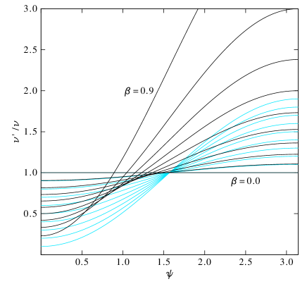
Figure 27: Graphical representation of (D.14) to demonstrate the “Comptonisation” effect: the relativistic Doppler-upshift for incident photons is larger in magnitude as the respective downshift for escaping photons. In contrast, the non-relativistic, classical Doppler shift is shown in light blue. It agrees with (D.14) but with $\gamma$ set to unity.

$$\omega(\frac{\mathbfl{\hat{k}}^{\mathsf{T}}\Delta\mathbfl{r}}{c}-\Delta t)=\omega^{\prime}(\frac{\Delta x^{\prime}\cos\psi^{\prime}}{c}+\frac{\Delta y^{\prime}\sin\psi^{\prime}}{c}-\Delta t^{\prime})$$

$$=\omega^{\prime}\gamma\,[\frac{(\Delta x-\beta c\Delta t)\cos\psi^{\prime}}{c}+\frac{\Delta y\sin\psi^{\prime}}{c}-(\Delta t-\frac{\beta}{c}\Delta x)]$$

$$=\omega^{\prime}\frac{\gamma}{c}\,[(\Delta x-\beta c\Delta t)\,\frac{\cos\psi-\beta}{1-\beta\cos\psi}+\Delta y\,\frac{\sin\psi}{\gamma(1-\beta\cos\psi)}-(c\Delta t-\beta\Delta x)]$$

$$=\omega^{\prime}\gamma\,[(1+\beta\frac{\cos\psi-\beta}{1-\beta\cos\psi})\Delta t-(\beta+\frac{\cos\psi-\beta}{1-\beta\cos\psi})\Delta x-\frac{\sin\psi}{\gamma(1-\beta\cos\psi)}\Delta y]$$

$$=\omega^{\prime}\gamma\,[\frac{(1-\beta^{2})\cos\psi}{1-\beta\cos\psi}\Delta x+\frac{\sin\psi}{\gamma(1-\beta\cos\psi)}\Delta y-\frac{1-\beta^{2}}{1-\beta\cos\psi}\Delta t]$$

$$=\frac{\omega^{\prime}}{\gamma(1-\beta\cos\psi)}[\cos\psi\Delta x-\sin\psi\Delta y-\Delta t]$$

$$\text{or}\quad\omega^{\prime}=\omega\gamma(1-\beta\cos\psi)$$ (D.14)

The reverse is immediately obtained if we use (D.10) to replace $\cos\psi$ by $\cos\psi^{\prime}$

$$\omega=\frac{\omega^{\prime}}{\gamma(1-\beta\cos\psi)}=\frac{\omega^{\prime}}{\gamma(1-\beta\frac{\cos\psi^{\prime}+\beta}{1+\beta\cos\psi^{\prime}})}$$

$$=\frac{\omega^{\prime}}{\gamma}\;\frac{1+\beta\cos\psi^{\prime}}{1+\beta\cos\psi^{\prime}-\beta(\cos\psi^{\prime}+\beta)}=\frac{\omega^{\prime}}{\gamma}\;\frac{1+\beta\cos\psi^{\prime}}{1-\beta^{2}}$$

$$=\omega^{\prime}\gamma(1+\beta\cos\psi^{\prime})$$ (D.15)

For convenience, we will introduce the Doppler shift factor $D$ as the “generic” version (D.14) of the frequency transformation

$$D(\mathbfl{\hat{k}},\boldsymbol{\beta})=\frac{1}{\gamma(1-\boldsymbol{\beta}^{\mathsf{T}}\mathbfl{\hat{k}})}$$ (D.16)

The convention is again that the arguments of $D$ including the relative velocity of the frames are measured in the same frame. If $\omega$ and $\mathbfl{k}$ are the photon frequency and wave vector in $S$ and $\mathbfl{v}=c\boldsymbol{beta}$ the velocity of $S^{\prime}$ in measured in $S$ then the Doppler-shifted frequency in frame $S^{\prime}$ is

$$\omega^{\prime}=\frac{\omega}{D(\mathbfl{\hat{k}},\boldsymbol{\beta})},\qquad\text{or reversely}\quad\omega=\frac{\omega^{\prime}}{D(\mathbfl{\hat{k}}^{\prime},-\boldsymbol{\beta})}$$ (D.17)

In both cases the observables in frames $S$ and $S^{\prime}$ are separated on the different sides of the equations. The minus sign in $D(\mathbfl{\hat{k}}^{\prime},-\boldsymbol{\beta})$ is needed because in frame $S^{\prime}$ the system $S$ of the left-hand-side moves with $-\mathbfl{v}$. We see immediately

$$D(\mathbfl{\hat{k}}^{\prime},-\boldsymbol{\beta})=\frac{1}{D(\mathbfl{\hat{k}},\boldsymbol{\beta})},\qquad D(-\mathbfl{\hat{k}},\boldsymbol{\beta})=D(\mathbfl{\hat{k}},-\boldsymbol{\beta}),$$

provided the directions $\mathbfl{\hat{k}}$ and $\mathbfl{\hat{k}^{\prime}}$ are appropriately related by aberration. The same frequency-shift conversion factor applies to the wave number because $\omega=ck$ and $\omega^{\prime}=ck^{\prime}$ must hold in each frame

$$k^{\prime}=\frac{k}{D(\mathbfl{\hat{k}},\boldsymbol{\beta})},\qquad k=\frac{k^{\prime}}{D(\mathbfl{\hat{k}}^{\prime},-\boldsymbol{\beta})}$$ (D.18)

D.3 Representation of the wave phase by the wave 4-vector

Define the the 4-vectors position and wave vector for a photon by $\vectf{r}=(ct,\mathbfl{r})^{\mathsf{T}}$ and $\vectf{k}=(\omega/c,\mathbfl{k})$. The momentum is related to the respective 4-wave vector by $\vectf{p}=\hbar\vectf{k}$. All 4-vectors are transformed by the Lorentz transformation (D.3) which we now rewrite independently from a coordinate system as a matrix to be multiplied to 4-vectors like $\vectf{r}$ or $\vectf{k}$. Here the first column is to be multiplied with the time component of a 4-vector, the second column has three components and is to be multiplied with its space components. In this form, the Lorentz transformation is

$$\vectf{L}=\begin{pmatrix}\gamma&-\gamma\boldsymbol{\beta}^{\mathsf{T}}\\ -\gamma\boldsymbol{\beta}&\boldsymbol{1}+(\gamma-1)\boldsymbol{\hat{\beta}}\boldsymbol{\hat{\beta}}{}^{\mathsf{T}}\end{pmatrix}\qquad\vectf{L}^{-1}=\begin{pmatrix}\gamma&\gamma\boldsymbol{\beta}^{\mathsf{T}}\\ \gamma\boldsymbol{\beta}&\boldsymbol{1}+(\gamma-1)\boldsymbol{\hat{\beta}}\boldsymbol{\hat{\beta}}{}^{\mathsf{T}}\end{pmatrix}$$

The transformation of $\vectf{r}$ and $\vectf{k}$ yield

$$\vectf{r}^{\prime}=\vectf{L}\vectf{r}=\left(\begin{array}[]{c}\!\!\gamma(ct-\boldsymbol{\beta}^{\mathsf{T}}\mathbfl{r})\!\!\\ \!\!(\boldsymbol{1}-\boldsymbol{\hat{\beta}}\boldsymbol{\hat{\beta}}{}^{\mathsf{T}})\mathbfl{r}+\gamma\boldsymbol{\hat{\beta}}(\boldsymbol{\hat{\beta}}{}^{\mathsf{T}}\mathbfl{r}-\beta ct)\!\!\end{array}\right)$$

$$\vectf{k}^{\prime}=\vectf{L}\vectf{k}=\left(\begin{array}[]{c}\!\!\gamma(\frac{\omega}{c}-\boldsymbol{\beta}^{\mathsf{T}}\mathbfl{k})\!\!\\ \!\!(\boldsymbol{1}-\boldsymbol{\hat{\beta}}\boldsymbol{\hat{\beta}}{}^{\mathsf{T}})\mathbfl{k}+\gamma\boldsymbol{\hat{\beta}}(\boldsymbol{\hat{\beta}}{}^{\mathsf{T}}\mathbfl{k}-\beta\frac{\omega}{c})\!\!\end{array}\right)$$

The product of $\vectf{r}^{\prime}$ and $\vectf{k}^{\prime}$ yields the same wave phase as $\vectf{k}^{\mathsf{T}}\vectf{r}$

$$\vectf{k}^{\prime}{}^{\mathsf{T}}\vectf{r}^{\prime}=-\gamma^{2}(ct-\boldsymbol{\beta}^{\mathsf{T}}\mathbfl{r})(\frac{\omega}{c}-\boldsymbol{\beta}^{\mathsf{T}}\mathbfl{k})$$

$$+[(\boldsymbol{1}-\boldsymbol{\hat{\beta}}\boldsymbol{\hat{\beta}}{}^{\mathsf{T}})\mathbfl{r}+\gamma\boldsymbol{\hat{\beta}}(\boldsymbol{\hat{\beta}}{}^{\mathsf{T}}\mathbfl{r}-\beta ct)[(\boldsymbol{1}-\boldsymbol{\hat{\beta}}\boldsymbol{\hat{\beta}}{}^{\mathsf{T}})\mathbfl{k}+\gamma\boldsymbol{\hat{\beta}}(\boldsymbol{\hat{\beta}}{}^{\mathsf{T}}\mathbfl{r}-\beta\frac{\omega}{c})]$$

$$=-\gamma^{2}(ct-\boldsymbol{\beta}^{\mathsf{T}}\mathbfl{r})(\frac{\omega}{c}-\boldsymbol{\beta}^{\mathsf{T}}\mathbfl{k})+\mathbfl{k}^{\mathsf{T}}(\boldsymbol{1}-\boldsymbol{\hat{\beta}}\boldsymbol{\hat{\beta}}{}^{\mathsf{T}})\mathbfl{r}+\gamma^{2}(\boldsymbol{\hat{\beta}}{}^{\mathsf{T}}\mathbfl{r}-\beta ct)(\boldsymbol{\hat{\beta}}{}^{\mathsf{T}}\mathbfl{r}-\beta\frac{\omega}{c})$$

$$=-\gamma^{2}(\omega t+\mathbfl{k}^{\mathsf{T}}\boldsymbol{\beta}\boldsymbol{\beta}^{\mathsf{T}}\mathbfl{r})+\gamma^{2}(\frac{\omega}{c}\boldsymbol{\beta}^{\mathsf{T}}\mathbfl{r}+ct\boldsymbol{\beta}^{\mathsf{T}}\mathbfl{k})$$

$$+\mathbfl{k}^{\mathsf{T}}(\boldsymbol{1}-\boldsymbol{\hat{\beta}}\boldsymbol{\hat{\beta}}{}^{\mathsf{T}})\mathbfl{r}+\gamma^{2}(\mathbfl{k}\boldsymbol{\hat{\beta}}\boldsymbol{\hat{\beta}}{}^{\mathsf{T}}\mathbfl{r}+\beta^{2}\omega t)-\gamma^{2}(\frac{\omega}{c}\boldsymbol{\beta}^{\mathsf{T}}\mathbfl{r}+ct\boldsymbol{\beta}^{\mathsf{T}}\mathbfl{k})$$

$$=-\gamma^{2}(1-\beta^{2})\omega t+\mathbfl{k}^{\mathsf{T}}(\boldsymbol{1}-\boldsymbol{\hat{\beta}}\boldsymbol{\hat{\beta}}{}^{\mathsf{T}})\mathbfl{r}+\gamma^{2}(1-\beta^{2})\mathbfl{k}\boldsymbol{\hat{\beta}}\boldsymbol{\hat{\beta}}{}^{\mathsf{T}}\mathbfl{r}$$

$$=-\omega t+\mathbfl{k}^{\mathsf{T}}\mathbfl{r}=\vectf{k}^{\mathsf{T}}\vectf{r}$$

Hence the Lorentz transformation does not effect 4-vector products. Moreover, we find again the laws for frequency shift and wave vector aberration in the expression of the transformed $\vectf{k}^{\prime}$. The first row in $\vectf{k}^{\prime}$ yields the frequency shift (D.14)

$$\omega^{\prime}=\gamma(\omega-c\beta k\cos\psi)=\gamma(1-\beta\cos\psi)\omega=\frac{\omega}{D(\mathbfl{\hat{k}},\boldsymbol{\beta})}$$

The second row yields the wave vector transformation

$$\mathbfl{k}^{\prime}=\mathbfl{k}+(\gamma-1)\boldsymbol{\hat{\beta}}\boldsymbol{\hat{\beta}}{}^{\mathsf{T}}\mathbfl{k}-\gamma\frac{\omega}{c}\boldsymbol{\beta}=\mathbfl{k}+(\gamma-1)\boldsymbol{\hat{\beta}}\boldsymbol{\hat{\beta}}{}^{\mathsf{T}}\mathbfl{k}-\gamma k\boldsymbol{\beta}$$ (D.19)

For the Jacobian of this wave vector transformation we find

$$\frac{d^{3}\mathbfl{k}^{\prime}}{d^{3}\mathbfl{k}}=\boldsymbol{1}+(\gamma-1)\frac{\boldsymbol{\beta}\boldsymbol{\beta}^{\mathsf{T}}}{\beta^{2}}-\gamma\boldsymbol{\beta}\mathbfl{\hat{k}}^{\mathsf{T}}\quad\text{with determinant}$$

$$\mathrm{det}(\frac{d^{3}\mathbfl{k}^{\prime}}{d^{3}\mathbfl{k}})=\gamma(1-\beta\cos\psi)=\frac{1}{D(\mathbfl{\hat{k}},\boldsymbol{\beta})}$$ (D.20)

To derive the determinant, we can without restriction let $\boldsymbol{\beta}$ point along $\mathbfl{\hat{x}}$ and place $\mathbfl{k}$ into the ($x,y$) plane.

Further manipulating (D.19) we have

$$\mathbfl{k}^{\prime}=(\boldsymbol{1}-\boldsymbol{\hat{\beta}}\boldsymbol{\hat{\beta}}{}^{\mathsf{T}})\mathbfl{k}+\gamma\boldsymbol{\hat{\beta}}(\boldsymbol{\hat{\beta}}{}^{\mathsf{T}}\mathbfl{k}-\beta k)=(\boldsymbol{1}-\boldsymbol{\hat{\beta}}\boldsymbol{\hat{\beta}}{}^{\mathsf{T}})\mathbfl{k}+\gamma k\boldsymbol{\hat{\beta}}(\cos\psi-\beta)$$ (D.21)

We see for once that the projection of the wave vector perpendicular to $\boldsymbol{\hat{\beta}}$ remains unaffected by the transformation

$$(\boldsymbol{1}-\boldsymbol{\hat{\beta}}\boldsymbol{\hat{\beta}}{}^{\mathsf{T}})\,\mathbfl{k}^{\prime}=(\boldsymbol{1}-\boldsymbol{\hat{\beta}}\boldsymbol{\hat{\beta}}{}^{\mathsf{T}})\,\mathbfl{k}$$ (D.22)

and for the component along $\boldsymbol{\hat{\beta}}$ we find

$$\mathbfl{k}^{\prime}{}^{\mathsf{T}}\boldsymbol{\hat{\beta}}=k^{\prime}\cos\psi^{\prime}=\gamma k(\cos\psi-\beta)$$

$$\text{and finally}\quad\cos\psi^{\prime}=\gamma\frac{k}{k^{\prime}}(\cos\psi-\beta)=\gamma D(\mathbfl{\hat{k}},\boldsymbol{\beta})(\cos\psi-\beta)=\frac{\cos\psi-\beta}{1-\beta\cos\psi}$$

where we used (D.18) in the last step to reobtain the aberration law (D.11).

The aberration formulas (D.12) and (D.11) can be rewritten independent from a coordinate system

$$\mathbfl{\hat{k}^{\prime}}{}^{\mathsf{T}}\boldsymbol{\hat{\beta}}=\gamma D(\mathbfl{\hat{k}},\boldsymbol{\beta})(\mathbfl{\hat{k}}^{\mathsf{T}}\boldsymbol{\hat{\beta}}-\beta), \quad\mathbfl{\hat{k}}^{\mathsf{T}}\boldsymbol{\hat{\beta}}=\gamma D(\mathbfl{\hat{k}}^{\prime},-\boldsymbol{\beta})(\mathbfl{\hat{k}^{\prime}}{}^{\mathsf{T}}\boldsymbol{\hat{\beta}}+\beta)$$

$$\text{or}\quad\mathbfl{k^{\prime}}{}^{\mathsf{T}}\boldsymbol{\hat{\beta}}=\gamma(\mathbfl{k}^{\mathsf{T}}\boldsymbol{\hat{\beta}}-k\beta), \quad\mathbfl{k}^{\mathsf{T}}\boldsymbol{\hat{\beta}}=\gamma(\mathbfl{k^{\prime}}{}^{\mathsf{T}}\boldsymbol{\hat{\beta}}+k^{\prime}\beta)$$ (D.23)

D.4 Transformation of the wave field

While aberration and frequency shift are derived in many standard textbooks on special relativity, the Lorentz transformation of the photon polarisation is seldomly considered. In fact, [Cocke and Holm, 1972] seems to be the first paper devoted to this problem. More recent treatments with applications to Gamma-ray bursts can be found in [Lyutikov et al., 2003, Nalewajko, 2009].

Consider a linearly polarised wave, either polarised in the aberration plane or normal to it. Recall that the aberration plane is spanned by the relative speed $\mathbfl{v}$ of reference frame $S^{\prime}$ seen in $S$ and the propagation directions $\mathbfl{\hat{k}}^{\prime}$ and $\mathbfl{\hat{k}}$ of the photon in $S^{\prime}$ and $S$, respectively. The aberration plane is identical in both frames and a polarisation in the plane or normal to it should be equally well identified in both systems. The mapping factors of the two polarisation amplitudes is, however, not immediately obvious.

We define a local right-handed, orthogonal coordinate system $\mathbfl{\hat{e}}_{1}$, $\mathbfl{\hat{e}}_{2}$ and $\mathbfl{\hat{e}}_{3}=\mathbfl{\hat{k}}$ attached to the photon in reference frame $S$. The photon electric field amplitude can be specified by

$$\mathbfl{E}{k}(\mathbfl{r},t)=E_{\mathbfl{k},1}(\mathbfl{r},t)\mathbfl{\hat{e}}_{1}+E_{\mathbfl{k},2}(\mathbfl{r},t)\mathbfl{\hat{e}}_{2}$$

The respective magnetic wave field is $\mathbfl{B}{k}=\mathbfl{\hat{k}}/c\times\mathbfl{E}{k}$ or

$$c\mathbfl{B}{k}(\mathbfl{r},t)=-E_{\mathbfl{k},2}(\mathbfl{r},t)\mathbfl{\hat{e}}_{1}+E_{\mathbfl{k},1}(\mathbfl{r},t)\mathbfl{\hat{e}}_{2}$$

We want to transform the photon to the frame $S^{\prime}$ which moves with $\mathbfl{v}=v\mathbfl{\hat{x}}=c\beta\mathbfl{\hat{x}}$. We use the freedom to rotate the polarisation directions $\mathbfl{\hat{e}}_{1}$ and $\mathbfl{\hat{e}}_{2}$ such that the aberration plane is spanned by $\mathbfl{\hat{e}}_{1}$ and $\mathbfl{\hat{e}}_{3}=\mathbfl{\hat{k}}$ and $\mathbfl{\hat{e}}_{2}$ is normal to the plane. With angle $\psi$ defined as in Fig. 24, we can decompose

$$\mathbfl{\hat{k}}=\cos\psi\mathbfl{\hat{x}}+\sin\psi\mathbfl{\hat{y}},\quad \mathbfl{\hat{e}}_{1}=\sin\psi\mathbfl{\hat{x}}-\cos\psi\mathbfl{\hat{y}},\quad\mathbfl{\hat{e}}_{2}=-\mathbfl{\hat{z}}$$ (D.24)

$$\mathbfl{\hat{x}}=\cos\psi\mathbfl{\hat{k}}+\sin\psi\mathbfl{\hat{e}}_{1},\quad \mathbfl{\hat{y}}=\sin\psi\mathbfl{\hat{k}}-\cos\psi\mathbfl{\hat{e}}_{1}$$

In this rotated frame the wave field is

$$\mathbfl{E}{k}=E_{\mathbfl{k},1}(\sin\psi\mathbfl{\hat{x}}-\cos\psi\mathbfl{\hat{y}})-E_{\mathbfl{k},2}\mathbfl{\hat{z}}$$

$$c\mathbfl{B}{\hat{k}}=-E_{\mathbfl{k},2}(\sin\psi\mathbfl{\hat{x}}-\cos\psi\mathbfl{\hat{y}})-E_{\mathbfl{k},1}\mathbfl{\hat{z}}$$

The electric field is transformed into $S^{\prime}$ by [Jackson, 1998, p. 558]

$$E^{\prime}_{\mathbfl{k}^{\prime},x}=E_{\mathbfl{k},x}=\sin\psi E_{\mathbfl{k},1} =\gamma(1-\beta\cos\psi)\sin\psi^{\prime}\;E_{\mathbfl{k},1}=\frac{\sin\psi^{\prime}}{D(\mathbfl{\hat{k}},\boldsymbol{\beta})}E_{\mathbfl{k},1}$$

$$E^{\prime}_{\mathbfl{k}^{\prime},y}=\gamma(E_{\mathbfl{k},y}-c\beta B_{\mathbfl{k},z}) =-\gamma(\cos\psi-\beta)E_{\mathbfl{k},1}=-\frac{\cos\psi^{\prime}}{D(\mathbfl{\hat{k}},\boldsymbol{\beta})}E_{\mathbfl{k},1}$$

$$E^{\prime}_{\mathbfl{k}^{\prime},z}=\gamma(E_{\mathbfl{k},z}+c\beta B_{\mathbfl{k},y}) =-\gamma(1-\beta\cos\psi)E_{\mathbfl{k},2}=-\frac{E_{\mathbfl{k},2}}{D(\mathbfl{\hat{k}},\boldsymbol{\beta})}$$

where for the last steps we used (D.12) and (D.11) for $E^{\prime}_{\mathbfl{k}^{\prime},x}$ and $E^{\prime}_{\mathbfl{k}^{\prime},y}$, respectively. In the moving frame $S^{\prime}$, we have the wave field component $E^{\prime}_{\mathbfl{k}^{\prime},z}$ normal to the aberration plane and the vector $E^{\prime}_{\mathbfl{k}^{\prime},x}\mathbfl{\hat{x}}+E^{\prime}_{\mathbfl{k}^{\prime},y}\mathbfl{\hat{y}}$ in the aberration plane. The transformation $S\longrightarrow S^{\prime}$ can thus be summarised by

$$\text{normal to aberration plane:}\quad\mathbfl{\hat{e}}_{2}^{\mathsf{T}}\mathbfl{E}_{\mathbfl{k}}=E_{\mathbfl{k},2}\quad \xrightarrow{S\rightarrow S^{\prime}}\quad\mathbfl{\hat{e}}_{2}^{\mathsf{T}}\mathbfl{E}^{\prime}_{\mathbfl{k}^{\prime}}=\frac{E_{\mathbfl{k},2}}{D(\mathbfl{\hat{k}},\boldsymbol{\beta})}$$ (D.25)

$$\text{in the aberration plane:}\hskip 35.00005pt(\boldsymbol{1}-\mathbfl{\hat{e}}_{2}\mathbfl{\hat{e}}_{2}^{\mathsf{T}})\mathbfl{E}{k} =E_{\mathbfl{k},1}\mathbfl{\hat{e}}_{1}=(\sin\psi\mathbfl{\hat{x}}-\cos\psi\mathbfl{\hat{y}})E_{\mathbfl{k},1}\hskip 100.00015pt$$

$$\quad\xrightarrow{S\rightarrow S^{\prime}}\quad(\boldsymbol{1}-\mathbfl{\hat{e}}_{2}\mathbfl{\hat{e}}_{2}^{\mathsf{T}})\mathbfl{E}^{\prime}_{\mathbfl{k}^{\prime}} =(\sin\psi\mathbfl{\hat{x}}-\gamma(\cos\psi-\beta)\mathbfl{\hat{y}})E_{\mathbfl{k},1}$$

$$=(\sin\psi^{\prime}\mathbfl{\hat{x}}-\cos\psi^{\prime}\mathbfl{\hat{y}})\frac{E_{\mathbfl{k},1}}{D(\mathbfl{\hat{k}},\boldsymbol{\beta})}$$ (D.26)

In the last step we used (D.10) and (D.9). Hence the field components in the aberration plane and normal to it are both modified in strength by the same factor $D^{-1}(\mathbfl{\hat{k}},\boldsymbol{\beta})$ and the aberrated field vector is tilted exactly so that it becomes normal to the aberrated propagation direction $\mathbfl{\hat{k}^{\prime}}$.

D.5 Transformations of irradiance and radiance

The energy density, the Poynting flux of a monochromatic wave and the irradiance transform according to (D.25) and (D.26) from the previous section as

$$W^{\prime}{k^{\prime}}=\frac{W{k}}{D^{2}(\mathbfl{\hat{k}},\boldsymbol{\beta})},\quad\mathbfl{S}^{\prime}_{\mathbfl{k}^{\prime}}=\frac{\mathbfl{S}{k}}{D^{2}(\mathbfl{\hat{k}},\boldsymbol{\beta})}$$

$$Q^{\prime}(\mathbfl{r}^{\prime},t^{\prime})=c\epsilon_{0}<\!\mathbfl{E}^{\prime}(\mathbfl{r}^{\prime},t^{\prime})^{\mathsf{T}}\mathbfl{E}^{\prime}(\mathbfl{r}^{\prime},t^{\prime})\!>=\frac{Q(\mathbfl{r},t)}{D^{2}(\mathbfl{\hat{k}},\boldsymbol{\beta})}$$

where $\mathbfl{k}$ and $\mathbfl{k}^{\prime}$ are related by aberration. For the spectral energy density and the spectral Poynting flux of a spectral distribution of waves we have to take into account that wave vectors transform differently depending on their propagation direction. Using (D.18) we have for an element in wave vector space

$$d^{3}\mathbfl{k}^{\prime}={k^{\prime}}^{2}dk^{\prime}d\Omega^{\prime}=\frac{k^{2}dk}{D^{3}(\mathbfl{\hat{k}},\boldsymbol{\beta})}d\Omega^{\prime}$$

For the transformation of the solid angle we find since the azimuthal angle $\phi=\phi^{\prime}$ remains invariant so that

$$d\Omega^{\prime}=\sin\psi^{\prime}d\psi^{\prime}d\phi^{\prime}=\frac{d\cos^{\prime}\psi}{d\cos\psi}\sin\psi d\psi d\phi=\frac{d}{d\cos\psi}(\frac{\cos\psi-\beta}{1-\beta\cos\psi})\;d\Omega$$

$$=(\frac{1}{1-\beta\cos\psi}+\frac{\beta(\cos\psi-\beta)}{(1-\beta\cos\psi)^{2}})\;d\Omega=\frac{(1-\beta\cos\psi)+\beta(\cos\psi-\beta)}{(1-\beta\cos\psi)^{2}}\;d\Omega$$

$$=\frac{1-\beta^{2}}{(1-\beta\cos\psi)^{2}}\;d\Omega=D^{2}(\mathbfl{\hat{k}},\boldsymbol{\beta})\;d\Omega$$ (D.27)

In total, the element in wave vector space therefore transforms as

$$d^{3}\mathbfl{k}^{\prime}=\frac{k^{2}dkd\Omega}{D(\mathbfl{\hat{k}},\boldsymbol{\beta})}=\frac{d^{3}\mathbfl{k}}{D(\mathbfl{\hat{k}},\boldsymbol{\beta})}$$ (D.28)

which agrees with (D.20) derived by different means above. Since $w(\mathbfl{k})d^{3}\mathbfl{k}$ has to transform as $W{k}$, we conclude

$$w^{\prime}(\mathbfl{k}^{\prime})d^{3}\mathbfl{k}^{\prime}=\frac{w(\mathbfl{k})d^{3}\mathbfl{k}}{D^{2}(\mathbfl{\hat{k}},\boldsymbol{\beta})}=\frac{w(\mathbfl{k})}{D(\mathbfl{\hat{k}},\boldsymbol{\beta})}\;\frac{d^{3}\mathbfl{k}}{D(\mathbfl{\hat{k}},\boldsymbol{\beta})}\quad\text{or}\quad w^{\prime}(\mathbfl{k}^{\prime})=\frac{w(\mathbfl{k})}{D(\mathbfl{\hat{k}},\boldsymbol{\beta})}$$

Similar reasoning leads to the transformed radiance [see Weiskopf et al., 1999, for a different derivation]

$$L^{\prime}(\mathbfl{\hat{k}^{\prime}})=\int w(k^{\prime}\mathbfl{\hat{k}^{\prime}})\;{k^{\prime}}^{2}\,dk^{\prime}=\int\frac{w(k\mathbfl{\hat{k}})}{D(\mathbfl{\hat{k}},\boldsymbol{\beta})}\;\frac{k^{2}\,dk}{D^{3}(\mathbfl{\hat{k}},\boldsymbol{\beta})}=\frac{L(\mathbfl{\hat{k}})}{D^{4}(\mathbfl{\hat{k}},\boldsymbol{\beta})}$$ (D.29)

while the irradiance

$$Q^{\prime}=\int L^{\prime}(\mathbfl{\hat{k}^{\prime}})d\Omega^{\prime}=\int\frac{L(\mathbfl{\hat{k}})}{D^{4}(\mathbfl{\hat{k}},\boldsymbol{\beta})}\;D^{2}(\mathbfl{\hat{k}},\boldsymbol{\beta})d\Omega=\frac{Q}{D^{2}(\mathbfl{\hat{k}},\boldsymbol{\beta})}$$ (D.30)

transforms like the field energy density as we have seen already above. Let $(ct_{\mathrm{em}},\mathbfl{r}_{\mathrm{em}})$ be the event of photon emission and $(ct_{\mathrm{in}},\mathbfl{r}_{\mathrm{in}})$ the event of its detection. Then we have for the world line between these two events

$$c^{2}(t_{\mathrm{in}}-t_{\mathrm{em}})^{2}-|\mathbfl{r}_{\mathrm{in}}-\mathbfl{r}_{\mathrm{em}}|^{2}=(c\Delta t)^{2}-d^{2}=0$$

in all frames. Hence the travel time $\Delta t$ of a photon transforms in the same way as the distance $d$ between the (retarded) position of the source and the detector. From (D.2) we have between two events in the moving system

$$c\Delta t^{\prime}=\gamma(c\Delta t-\boldsymbol{\beta}^{\mathsf{T}}\Delta\mathbfl{r})$$

For the events photon emission and detection we have a spatial distance of $\Delta\mathbfl{r}=\mathbfl{\hat{k}}\,d=\mathbfl{\hat{k}}c\Delta t$. This yields the transformation of the travel time $\Delta t$ and the same transformation for the distance $d$

$$c\Delta t^{\prime}=\frac{c\Delta t}{D(\mathbfl{\hat{k}},\boldsymbol{\beta})},\qquad d^{\prime}=\frac{d}{D(\mathbfl{\hat{k}},\boldsymbol{\beta})}$$ (D.31)

Accordingly, the radiant intensity of a point source transforms like

$$I^{\prime}(\mathbfl{\hat{k}^{\prime}})=Q^{\prime}(\mathbfl{r}^{\prime}_{\mathrm{em}}+d^{\prime}\mathbfl{\hat{k}^{\prime}}){d^{\prime}}^{2}=\frac{Q(\mathbfl{r}_{\mathrm{em}}+\mathbfl{\hat{k}}\,d)}{D^{2}(\mathbfl{\hat{k}},\boldsymbol{\beta})}\frac{d^{2}}{D^{2}(\mathbfl{\hat{k}},\boldsymbol{\beta})}=\frac{I(\mathbfl{\hat{k}})}{D^{4}(\mathbfl{\hat{k}},\boldsymbol{\beta})}$$ (D.32)

The above relations have been derived previously and discussed in detail [McKinley, 1979, 1980, Eriksen and Grøn, 1992, Kraus, 2000]. Their derivation is, however, different from our approach by associating. There, the radiance is associated by a particle stream of photons, the world lines of which are transformed between frames and the resulting count rates on a detector surface in the different frames are compared.

D.6 Relativistic equilibrium velocity distribution

Both relativistic invariance and thermodynamic equilibrium are difficult to reconcile. Since Jüttner’s first publication on this topic a century ago [Jüttner, 1911], it has been discussed in a series of papers and textbook contributions without that a final consensus seems to have emerged. A full account of the topic is therefore beyond the scope of this manuscript. A through discussion on the state of art can be found in [Debbasch, 2008]. Here, we follow essentially the approach of Lehmann [2006].

Define $\vectf{r}=(ct,\mathbfl{r})$ and $\vectf{p}=(E,c\mathbfl{p})$ as 4-vectors for position and momentum of an electron. The space component of the momentum is related to velocity by $\mathbfl{p}=\gamma m_{e}c\boldsymbol{\beta}$. In order to obtain a relativistic invariant distribution function, all dependencies on $\vectf{r}$ and $\vectf{p}$ should be wrapped into invariant 4-vector products. We neglect interactions and we can therefore just consider a single particle distribution. For free particles an invariant extension of Maxwell’s distribution is

$$f(\mathbfl{p})\;d^{3}\mathbfl{r}d^{3}c\mathbfl{p}=\frac{d\Gamma}{Z(T,\vectf{u})}\exp(-\frac{\vectf{u}^{\mathsf{T}}\vectf{p}}{k_{B}T})$$

$$d\Gamma=\int d\compf{r}^{0}\int_{0}^{\infty}d\compf{p}_{0}\;\prod_{\alpha=1}^{3}d\compf{r}^{\alpha}d\compf{p}_{\alpha}\delta(g_{1}(\vectf{r},\vectf{p}))\delta(g_{2}(\vectf{r},\vectf{p}))$$

where $\vectf{u}=(1,\mathbfl{u}/c)$ is the velocity 4-vector of the system so that $\vectf{u}^{\mathsf{T}}\vectf{p}$ is invariant, $T$ is the system temperature and $Z(T,\vectf{u})$ the partition function. The distribution function should be homogeneous and stationary, i.e., it should not depend on $\vectf{r}$ at all. In the phase space element $d\Gamma$, all 8 components of $\vectf{r}$ and $\vectf{p}$ are independent variables. The $\delta$-functions in the phase space element $d\Gamma$ aim at reducing the 8-dimensional phase space to the usual 6 dimensions by constraining time and energy. The choice for $g_{1}$ is obvious, it must enforce the electron’s energy-momentum relation

$$g_{1}=\vectf{p}^{\mathsf{T}}\vectf{p}-m_{e}^{2}c^{4}=E^{2}-c^{2}\mathbfl{p}^{2}=E^{2}-m_{e}^{2}c^{4}(\gamma^{2}\boldsymbol{\beta}^{2}+1)=E^{2}-\gamma^{2}m_{e}^{2}c^{4}$$

For $g_{1}$ several variants could be considered:

Lehmann’s invariant $$g_{2}^{\mathrm{L}} =\vectf{r}^{\mathsf{T}}\vectf{p}-m_{e}^{2}c^{3}\tau=cEt-c\mathbfl{r}^{\mathsf{T}}\mathbfl{p}-m_{e}c^{2}\tau$$

$$=m_{e}c^{2}\gamma(ct-\mathbfl{r}^{\mathsf{T}}\boldsymbol{\beta})-m_{e}c^{3}\tau$$

Inhomogeneous invariant $$g_{2}^{\mathrm{I}} =\vectf{r}^{\mathsf{T}}\vectf{r}-(c\tau)^{2}=(ct)^{2}-\mathbfl{r}^{2}-(c\tau)^{2}$$

Jüttner non-invariant $$g_{2}^{\mathrm{J}} =\frac{R_{0}}{\gamma}-c\tau=\frac{ct}{\gamma}-c\tau$$

Plain non-invariant $$g_{2}^{\mathrm{P}} =R_{0}-c\tau=c(t-\tau)$$

For the first three cases, the condition $g_{2}=0$ restricts the $\vectf{r}$ integration which is finally required to determine the partition function to a time-like hyperbola in Minkowski space which intersects the time axis at $ct=c\tau$. Hence parameter $\tau$ is the eigentime of a particle regardless of its velocity. In a frame where the particle has velocity $\boldsymbol{\beta}$ and starts from the origin it is located at $(ct,\mathbfl{r})$ after its own time $\tau$. Even though all three $g_{2}$ have the same roots in Minkowski space and enforce the same constraint on the four components of $\vectf{r}$, they intersect the root with different first derivative which inflicts differences for the integration. The fourth case is clearly not invariant as it ignores the differences between time and eigentime.

When integrating over the energy and time constraints, we have to obey the following rules. If $x_{i}$ are the roots of $g(x)$

$$\int_{0}^{\infty}dx\;\delta(g(x))h(x)=\sum_{i}\frac{1}{g^{\prime}(x_{i})}h(x_{i})$$

$g_{1}$ has two roots $\compf{p}_{0}=E$ but the negative root is discarded by the restriction to positive free energies. Abbreviating $\exp(-\vectf{u}^{\mathsf{T}}\vectf{p}/k_{B}T)=h(\vectf{p})$ we find

$$\int_{0}^{\infty}d\compf{p}_{0}\;\delta(g_{1})h(\vectf{p})=\int_{0}^{\infty}dE\;\delta(E^{2}-\gamma^{2}m_{e}^{2}c^{4})\,h(E,c\mathbfl{p})$$

$$=\int_{0}^{\infty}dE\;\frac{\delta(E-\gamma m_{e}c^{2})}{2E}h(E,c\mathbfl{p})=\frac{h(\gamma m_{e}c^{2},c\mathbfl{p})}{2\gamma m_{e}c^{2}}$$

The integration over $\compf{r}_{0}$ yields for the different $g_{1}$ (we omit $h$ because it is independent on $\vectf{r}$)

$$\int_{0}^{\infty}d\compf{r}_{0}\;\delta(g_{2})=\int_{0}^{\infty}d(ct)\;\delta(g_{2})=\begin{cases}\displaystyle\frac{1}{E}=\frac{1}{\gamma m_{e}c^{2}}&\text{for}\;g_{2}^{\mathrm{L}}\\[6.45831pt] \displaystyle\frac{1}{2\sqrt{\mathbfl{r}^{2}+(c\tau)^{2}}}&\text{for}\;g_{2}^{\mathrm{I}}\\[4.30554pt] \hskip 30.00005pt\gamma&\text{for}\;g_{2}^{\mathrm{J}}\\ \hskip 30.00005pt1&\text{for}\;g_{2}^{\mathrm{P}}\end{cases}$$

We obviously have to discard $g_{L}^{\mathrm{I}}$ because it introduces a space dependence into the distribution function. To show dependencies more clearly we express $\gamma$ in terms of $\mathbfl{p}$ by

$$\gamma^{2}(\mathbfl{p})=1+\gamma^{2}\beta^{2}=1+\frac{\mathbfl{p}^{2}}{m_{e}^{2}c^{2}}$$ (D.33)

Insertion into (D.6) gives for the three remaining cases

$$f(\mathbfl{p})\;d^{3}\mathbfl{r}d^{3}\mathbfl{p}=\frac{d^{3}\mathbfl{p}\;d^{3}\mathbfl{r}}{Z(T,\vectf{u})}\exp(-\frac{\vectf{u}^{\mathsf{T}}(\gamma(\mathbfl{p})m_{e}c^{2},c\mathbfl{p})}{k_{B}T})\begin{cases}\displaystyle\frac{1}{2(\gamma(\mathbfl{p})m_{e}c^{2})^{2}}&\text{for}\;g_{2}^{\mathrm{L}}\\[8.61108pt] \displaystyle\hskip 20.00003pt\frac{1}{2m_{e}c^{2}}&\text{for}\;g_{2}^{\mathrm{J}}\\[8.61108pt] \displaystyle\hskip 10.00002pt\frac{1}{2\gamma(\mathbfl{p})m_{e}c^{2}}&\text{for}\;g_{2}^{\mathrm{P}}\end{cases}$$

$$=\frac{d^{3}\mathbfl{p}\;d^{3}\mathbfl{r}}{Z(T,\vectf{u})}\exp(-\frac{c\sqrt{\rule{0.0pt}{8.61108pt}(m_{e}c)^{2}+\mathbfl{p}^{2}}-\mathbfl{u}^{\mathsf{T}}\mathbfl{p}}{k_{B}T})\begin{cases}\displaystyle\frac{1}{2c^{2}((m_{e}c)^{2}+\mathbfl{p}^{2})}&\text{for}\;g_{2}^{\mathrm{L}}\\[8.61108pt] \displaystyle\hskip 25.00003pt\frac{1}{2m_{e}c^{2}}&\text{for}\;g_{2}^{\mathrm{J}}\\[8.61108pt] \displaystyle\frac{1}{2c\sqrt{\rule{0.0pt}{6.45831pt}(m_{e}c)^{2}+\mathbfl{p}^{2}}}&\text{for}\;g_{2}^{\mathrm{P}}\end{cases}$$

We see that depending on the choice of $g_{2}$ we obtain slightly different distribution functions. For $g_{2}^{L}$ we have relativistic invariance while Jüttner’s original distribution for $g_{2}^{J}$ is manifestly stationary because it commutes with the single particle Hamiltonian. In numerical simulations, a relativistic gas of virtual particles seems to approach the original Jüttner distribution. [Montakhab et al., 2009]. We will therefore use the Jüttner distribution for our calculations of Fig. 23.

Note that when we want to use the electron velocity $\boldsymbol{\beta}$ instead of the momentum $\mathbfl{p}$ as variable in the distribution function we have to insert $\mathbfl{p}=m_{e}c\gamma\boldsymbol{\beta}$ and also convert the momentum space element to the velocity space element

$$f(\mathbfl{p})\;d^{3}\mathbfl{r}d^{3}\mathbfl{p}=f(\frac{m_{e}c\boldsymbol{\beta}}{\sqrt{1-\beta^{2}}})\;|\det(\frac{d^{3}\mathbfl{p}}{d^{3}\boldsymbol{\beta}})|\;d^{3}\mathbfl{r}\,d^{3}\boldsymbol{\beta}$$

$$\frac{d^{3}\mathbfl{p}}{d^{3}\boldsymbol{\beta}}=m_{e}c\gamma(\boldsymbol{1}+\gamma^{2}\boldsymbol{\beta}\boldsymbol{\beta}^{\mathsf{T}})$$

$$\det(\frac{d^{3}\mathbfl{p}}{d^{3}\boldsymbol{\beta}})=(m_{e}c\gamma)^{3}(1+\gamma^{2}\beta^{2})=(m_{e}c)^{3}\gamma^{5}$$

It remains to calculate the respective partition function which guarantees the normalisation and it is also an important means to derive thermodynamic equilibrium quantities. We restrict its evaluation to the rest frame of the system, i.e., for $\mathbfl{u}=0$. Introducing $\rho^{2}=\mathbfl{p}^{2}/(m_{e}c)^{2}$ and $\Theta=m_{e}c^{2}/k_{B}T$ we obtain for the three different cases

$$Z(T,\vectf{u})=\int d^{3}\mathbfl{p}\;d^{3}\mathbfl{r}\exp(-\frac{c\sqrt{\rule{0.0pt}{6.45831pt}(m_{e}c)^{2}+\mathbfl{p}^{2}}}{k_{B}T})\begin{cases}\displaystyle\frac{1}{2c^{2}((m_{e}c)^{2}+\mathbfl{p}^{2})}&\text{for}\;g_{2}^{\mathrm{L}}\\[8.61108pt] \displaystyle\hskip 25.00003pt\frac{1}{2m_{e}c^{2}}&\text{for}\;g_{2}^{\mathrm{J}}\\[8.61108pt] \displaystyle\frac{1}{2c\sqrt{\rule{0.0pt}{6.45831pt}(m_{e}c)^{2}+\mathbfl{p}^{2}}}&\text{for}\;g_{2}^{\mathrm{P}}\end{cases}$$

$$=\frac{4\pi V}{2m_{e}c^{2}}\int_{0}^{\infty}d\rho\,\begin{Bmatrix}\displaystyle\frac{\rho^{2}}{m_{e}c^{2}\,(1+\rho^{2})}\\[9.90276pt] \rho^{2}\\[3.44444pt] \displaystyle\frac{\rho^{2}}{\sqrt{\rule{0.0pt}{6.45831pt}1+\rho^{2}}}\end{Bmatrix}\exp(-\Theta\sqrt{1+\rho^{2}})$$

$$=\frac{4\pi V}{2m_{e}c^{2}}\begin{cases}\displaystyle\frac{1}{m_{e}c^{2}}G(\Theta)\quad\text{with}\;G^{\prime}(\Theta)=\frac{1}{\Theta}K_{1}(\Theta)&\text{for}\;g_{2}^{\mathrm{L}}\\[6.45831pt] \displaystyle\frac{1}{\Theta}K_{2}(\Theta)={\textstyle\!\frac{1}{4}}(K_{3}(\Theta)-K_{1}(\Theta))&\text{for}\;g_{2}^{\mathrm{J}}\\[6.45831pt] \displaystyle\frac{1}{\Theta}K_{1}(\Theta)={\textstyle\!\frac{1}{2}}(K_{2}(\Theta)-K_{0}(\Theta))&\text{for}\;g_{2}^{\mathrm{P}}\end{cases}$$

To evaluate the integrals we used the integral representation of the modified Bessel functions of the second kind [Gradshteyn and Ryzhik, 1980, 8.432.3]

$$K_{\nu}(z)=K_{-\nu}(z)=\frac{\sqrt{\pi}}{\Gamma(\nu+{\textstyle\!\frac{1}{2}})}(\frac{z}{2})^{\nu}\int_{1}^{\infty}e^{-zy}(y^{2}-1)^{\nu-{\textstyle\!\frac{1}{2}}}\;dy$$ (D.34)

$$\text{with derivative}\quad K^{\prime}_{\nu}(z)=\frac{\nu}{z}K_{\nu}(z)-\frac{\sqrt{\pi}}{\Gamma(\nu+{\textstyle\!\frac{1}{2}})}(\frac{z}{2})^{\nu}\int_{1}^{\infty}e^{-zy}y(y^{2}-1)^{\nu-{\textstyle\!\frac{1}{2}}}\;dy$$ (D.35)

With the recurrence relations [Gradshteyn and Ryzhik, 1980, 8.486.10+11]

$$K_{\nu+1}(z)-K_{\nu-1}(z)=2\,\frac{\nu}{z}K_{\nu}(z)$$

$$K_{\nu+1}(z)+K_{\nu-1}(z)=-2\,K^{\prime}_{\nu}(z)$$

$$K^{\prime}_{\nu}\mp\frac{\nu}{z}K_{\nu}=\mp K_{\nu\pm 1}$$

$$\text{we find from (\ref{dKn0})}\qquad-(K^{\prime}_{\nu}(z)-\frac{\nu}{z}K_{\nu}(z))=K_{\nu+1}(z)$$

$$=\frac{\sqrt{\pi}}{\Gamma(\nu+{\textstyle\!\frac{1}{2}})}(\frac{z}{2})^{\nu}\int_{1}^{\infty}e^{-zy}y(y^{2}-1)^{\nu-{\textstyle\!\frac{1}{2}}}\;dy$$ (D.36)

From (D.34), (D.36) and $\Gamma{3/2}=\sqrt{\pi}/2$ for $\nu=1$

$$K_{1}(z)=z\int_{1}^{\infty}e^{-zy}\sqrt{y^{2}-1}\;dy$$

$$K_{2}(z)=z\int_{1}^{\infty}e^{-zy}y\sqrt{y^{2}-1}\;dy$$

So that

$$\int_{0}^{\infty}\frac{\rho^{2}}{\rule{0.0pt}{11.19443pt}\sqrt{\rule{0.0pt}{8.61108pt}1+\rho^{2}}^{\,\alpha}}\,e^{-z\sqrt{1+\rho^{2}}}\,d\rho\;\stackrel{{\scriptstyle\rho=\sinh\,t}}{{=}}\;\int_{0}^{\infty}\frac{\sinh^{2}t}{\cosh^{\alpha}t}\,e^{-z\cosh\,t}\,d(\sinh\,t)$$

$$=\int_{0}^{\infty}\sinh^{2}t\cosh^{1-\alpha}t\,e^{-z\cosh\,t}\,dt\;\stackrel{{\scriptstyle\cosh\,t=y}}{{=}}\;\int_{1}^{\infty}\sqrt{y^{2}-1}\;y^{1-\alpha}\;e^{-zy}\,dy$$

$$=\begin{cases}\displaystyle G(z)\;\text{with}\;G^{\prime}(z)=\frac{1}{z}K_{1}(z)&\text{for}\;\alpha=2\\ \displaystyle\hskip 30.00005pt\frac{1}{z}K_{2}(z)&\text{for}\;\alpha=0\\[6.45831pt] \displaystyle\hskip 30.00005pt\frac{1}{z}K_{1}(z)&\text{for}\;\alpha=1\\ \end{cases}$$

For $G(z)$ we did not find a simple expression. Taking account of the fact that $G(z)\rightarrow 0$ for $z\rightarrow\infty$ we can write $G(z)$ as [Rosenheinrich, 2015, p.20]

$$G(z)=\int_{z}^{\infty}\frac{K_{1}(z^{\prime})}{z^{\prime}}dz^{\prime}$$

$$=zK_{0}(z)+K_{1}(z)+\frac{\pi z}{2}(K_{0}(z)L_{1}(z)+K_{1}(z)L_{0}(z))$$

where

$$L_{n}(z)=(\frac{z}{2})^{n+1}\sum_{k=0}^{\infty}\frac{1}{\Gamma(k+3/2)\Gamma(k+n+3/2)}(\frac{z}{2})^{2k}$$

is the modified Struve function.

D.7 Lorentz transformation of space-cones and spheres

Due to the mixture of time and space coordinates, a Lorentz transformation (D.2) of extended objects from one frame to another is often not intuitive. Even more so is the instantaneous view which observers have on an object from different frames because different travel times of photons from different parts of the object have to be taken into into account. As a consequence, objects may appear considerably deformed from their rest frame shape. In this section we want to elucidate how the Sun appears to a relativistic coronal electron.

An exception from the above mentioned relativistic deformation are space-cones peaked at the observer. Such a 3D space-cone (not to be confused with a 4D light-cone) with its apex at $\mathbfl{r}_{\mathrm{obs}}$ is given in its rest frame $S$ by points $\mathbfl{r}$ which satisfy

$$(\mathbfl{r}-\mathbfl{r}_{\mathrm{obs}})^{\mathsf{T}}\mathbfl{\hat{a}}_{\theta}=|\mathbfl{r}-\mathbfl{r}_{\mathrm{obs}}|\cos\theta$$

where $\mathbfl{\hat{a}}_{\theta}$ is the unit direction of the cone axis of a cone of opening angle $\theta$. Photons received by the observer at $t=t_{\mathrm{in}}$ were emitted from $\mathbfl{r}$ at the retarded time $t=t_{\mathrm{in}}-|\mathbfl{r}-\mathbfl{r}_{\mathrm{obs}}|/c$. Therefore the space-time events $(ct,\mathbfl{r})$ of emitting photons from the cone surface which all arrive at $(ct_{\mathrm{in}},\mathbfl{r}_{\mathrm{obs}})=0$ are connected by the linear relation

$$ct\cos\theta+\mathbfl{r}^{\mathsf{T}}\mathbfl{\hat{a}}_{\theta}=0$$ (D.37)

If the observer collects the photons in a camera, he would observe the image of a circle with radius $\theta$ and the centre in direction $\mathbfl{\hat{a}}_{\theta}$. Aside from their geometrical meaning, we may consider $\cos\theta$ and $|\mathbfl{\hat{a}}_{\theta}|$ as general coefficients in (D.37) which represents a space-like cone as long as $|\mathbfl{\hat{a}}_{\theta}|>|\cos\theta|$.

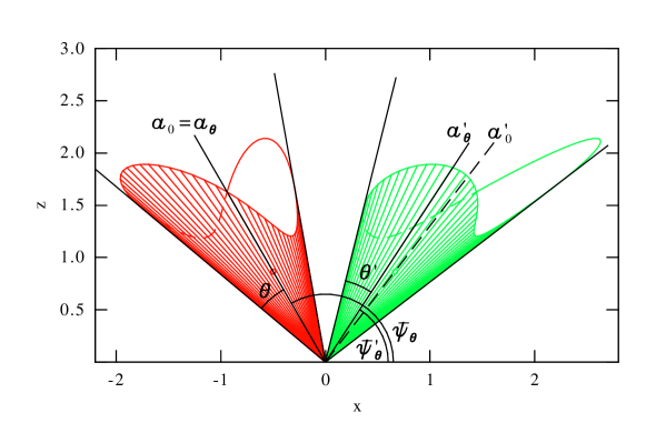
Figure 28: Lorentz transformation of a space cone from its rest fame (red) to a moving frame with $\beta=0.85$ to the right (green) for the observers in both frames at $\mathbfl{r}=\mathbfl{r}^{\prime}=0$ at the time of observation. Here, $\mathbfl{\hat{a}}_{\theta}$ and $\mathbfl{\hat{a}}_{0}$ are the directions of the cone centres for a finite opening angle $\theta$ and of a degenerated cone of zero opening, both aligned in the rest frame. For the observers, the finite width cones appear as circles centred in directions $\mathbfl{\hat{a}}_{\theta}$ (rest frame) and $\mathbfl{\hat{a}}^{\prime}_{\theta}$ (moving frame). In the moving frame, the cone centre $\mathbfl{\hat{a}}^{\prime}_{\theta}$ is not aligned any more with the aberrated direction $\mathbfl{\hat{a}}_{0}^{\prime}$ of the cone centre (indicated by a dashed line).

Consider another observer in a moving frame $S^{\prime}$ at $\mathbfl{r}^{\prime}_{\mathrm{obs}}=0$ such that the origins of $S$ and $S^{\prime}$ are the same at time $ct^{\prime}=ct=0$. Then the observer in the moving frame receives the same photons at $ct^{\prime}=0$ as the observer in $S$ at $ct=0$. However, in $S^{\prime}$ they have different travel times and were emitted form different coordinate positions. Applying the Lorentz transformation to (D.37) must give without explicit calculation

$$ct^{\prime}\cos\theta^{\prime}+\mathbfl{r}^{\prime}{}^{\mathsf{T}}\mathbfl{\hat{a}^{\prime}}_{\theta}=0$$ (D.38)

because the linear structure of (D.37) is maintained due to the linearity of the Lorentz transformation (D.2). So we obtain yet another cone in the new frame and the moving observer will receive the image of another circle provided the yet unknown coefficients in (D.38) obey $\cos\theta^{\prime}<|\mathbfl{\hat{a}^{\prime}}_{\theta}|$.

To obtain the explicit expressions for $\mathbfl{\hat{a}^{\prime}}_{\theta}$ and $\cos\theta^{\prime}$, we follow [Boas, 1961], apply the Lorentz transformation to (D.37) and reorder the terms to obtain a form as in (D.38). For convenience, we assume that in the rest frame the vector $\mathbfl{\hat{a}}_{\theta}$ lies in the $x,z$ plane and forms an angle $\bar{\psi}_{\theta}$ with the $\mathbfl{\hat{x}}$ axis. Then $\mathbfl{\hat{a}}_{\theta}=(\cos\bar{\psi}_{\theta},0,\sin\bar{\psi}_{\theta})$ and from (D.38).

$$ct\cos\theta+x\cos\bar{\psi}_{\theta}+z\sin\bar{\psi}_{\theta}=0\quad\xrightarrow{S\rightarrow S^{\prime}}$$

$$0=\gamma(ct^{\prime}+\beta x^{\prime})\cos\theta+\gamma(x^{\prime}+\beta ct^{\prime})\cos\bar{\psi}_{\theta}+z^{\prime}\sin\bar{\psi}_{\theta}$$

$$=\gamma(\cos\theta+\beta\cos\bar{\psi}_{\theta})ct^{\prime}+\gamma(\cos\bar{\psi}_{\theta}+\beta\cos\theta)x^{\prime}+z^{\prime}\sin\bar{\psi}_{\theta}$$

Comparison with (D.38) gives except for a common constant $$b$$

$$b\cos\theta^{\prime}=\gamma(\cos\theta+\beta\cos\bar{\psi}_{\theta}),\quad b\cos\bar{\psi}^{\prime}_{\theta}=\gamma(\cos\bar{\psi}_{\theta}+\beta\cos\theta),\quad b\sin\bar{\psi}^{\prime}_{\theta}=\sin\bar{\psi}_{\theta},\quad$$ (D.39)

$$1=\cos^{2}\bar{\psi}^{\prime}_{\theta}+\sin^{2}\bar{\psi}^{\prime}_{\theta}\quad\text{yields}\quad b^{2}=\gamma^{2}(\cos\bar{\psi}_{\theta}+\beta\cos\theta)^{2}+\sin^{2}\bar{\psi}_{\theta}$$ (D.40)

With this normalisation we readily find that $|\cos\theta^{\prime}|\leq 1$. We show that $b^{2}>b^{2}\cos^{2}\theta^{\prime}$ or

$$b^{2}-\gamma^{2}(\cos\theta+\beta\cos\bar{\psi}_{\theta})^{2}=\gamma^{2}(\cos\bar{\psi}_{\theta}+\beta\cos\theta)^{2}+\sin^{2}\bar{\psi}_{\theta}-\gamma^{2}(\cos\theta+\beta\cos\bar{\psi}_{\theta})^{2}$$

$$=\gamma^{2}\cos^{2}\bar{\psi}_{\theta}+\gamma^{2}\beta^{2}\cos^{2}\theta+2\gamma^{2}\beta\cos\bar{\psi}_{\theta}\cos\theta+\sin^{2}\bar{\psi}_{\theta}$$

$$-\gamma^{2}\cos^{2}\theta-\gamma^{2}\beta^{2}\cos^{2}\bar{\psi}_{\theta}-2\gamma^{2}\beta\cos\theta\cos\bar{\psi}_{\theta}$$

$$=\gamma^{2}(1-\beta^{2})\cos^{2}\bar{\psi}_{\theta}+\gamma^{2}(\beta^{2}-1)\cos^{2}\theta+\sin^{2}\bar{\psi}_{\theta}$$

$$=1-\cos^{2}\theta=\sin^{2}\theta\geq 0$$

and we can also write the normalisation (D.40) alternatively as

$$b^{2}=\gamma^{2}(\cos\theta+\beta\cos\bar{\psi}_{\theta})^{2}+\sin^{2}\theta$$ (D.41)

Obviously, the images which both observers take with this setup both show a circle, centred in direction $\mathbfl{\hat{a}}_{\theta}$ or $\mathbfl{\hat{a}}^{\prime}_{\theta}$ and with angular diameter $\theta$ or $\theta^{\prime}$, respectively. From (D.39) and (D.41) we have for the transformed cone

$$\cos\theta^{\prime}=\frac{(\cos\theta+\beta\cos\bar{\psi}_{\theta})}{\sqrt{(\cos\theta+\beta\cos\bar{\psi}_{\theta})^{2}+\sin^{2}\theta/\gamma^{2}}}$$

$$\cos\bar{\psi}^{\prime}_{\theta}=\frac{\cos\bar{\psi}_{\theta}+\beta\cos\theta}{\sqrt{(\cos\theta+\beta\cos\bar{\psi}_{\theta})^{2}+\sin^{2}\theta/\gamma^{2}}}$$ (D.42)

The situation is illustrated in Fig. 28. Note that the direction $\mathbfl{\hat{a}}^{\prime}_{\theta}=(\cos\bar{\psi}^{\prime}_{\theta},0,\sin\bar{\psi}^{\prime}_{\theta})$ of the cone centre in the moving frame is slightly shifted with respect to the aberrated direction of the cone axis, which we obtain if we compare the above results with a cone of opening $\theta=0$ but the same direction $\mathbfl{\hat{a}}_{0}=\mathbfl{\hat{a}}_{\theta}$ in the rest frame. The aberrated direction $\mathbfl{\hat{a}}^{\prime}_{0}$ of this degenerated cone axis is then

$$\cos\bar{\psi}^{\prime}_{0}=\frac{\cos\bar{\psi}_{0}+\beta}{1+\beta\cos\bar{\psi}_{0}}$$

which is, as expected, the aberration (D.13) for incoming photons. We will refer to this phenomenon as aberration shift of cone centres. It causes any space curve which projects as a circle to an observer in the rest frame to be seen by a moving observer from the same perspective as an aberrated circle with its apparent centre shifted with respect to the aberrated centre of the circle in the rest frame. This shift increases with the opening angle $\theta$ of the cone, or, equivalently with the radius of the observed circle and vanishes naturally if $\theta$ approaches zero (see Fig. 30 below).

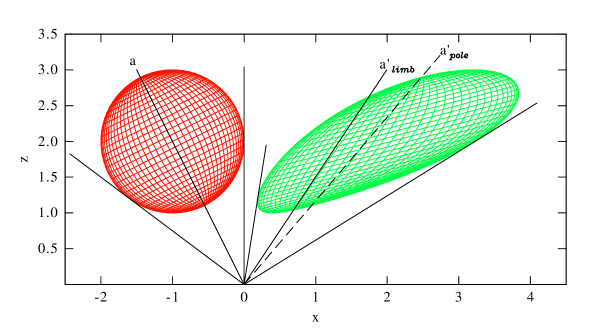
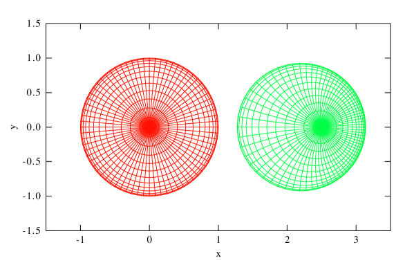
Figure 29: Lorentz transformation of a sphere from its rest frame (red) to a moving frame with $\beta=0.85$ along the $\mathbfl{\hat{x}}$-axis (green). The upper figure shows the transformed geometries from a side view with the observers at $(ct,\mathbfl{r})=(ct^{\prime},\mathbfl{r}^{\prime})=0$. The bottom panel shows the images the two observers would obtain in projective geometry with a camera oriented in direction to the centre of the respective limb circle.

We will now apply these results to the surface of a sphere with radius $R_{\odot}$. A natural coordinate system on the sphere’s surface in its rest frame has a $\mathbfl{\hat{z}}$-axis along the direction from the observer to the centre of the sphere which we will again call $\mathbfl{\hat{a}}$. Latitude circles on the sphere are then obtained as intersections of the sphere surface with cones defined above with the cone opening angle varying from $\theta=0$ (observer pole) to $\theta=\mathrm{asin}(R_{\odot}/r)$ (observer limb) where $r$ is the distance of the observer from the centre of the sphere in the rest frame. Note that distance $r$ and angle $\theta$ correspond to the notation in Fig. 4 if we assume that the observer is located at the scattering site. In Fig. 29 we give an example of how this sphere transforms into the frame of a moving observer located at the origin at the time of the observation. The upper diagram shows the sphere in its rest frame (red) and in the moving frame (green). The transformed sphere has been obtained by a Lorentz transformation of the space-time events $(ct=-|\mathbfl{r}|,\mathbfl{r})$ at which the received photons were emitted from the surface of the sphere. For the top perspective in Fig. 29 the sphere was assumed transparent so that a transform also for the backside of the sphere is obtained. Here $\mathbfl{\hat{a}}$ is the direction to the sphere centre and to the observer pole in the rest frame. It transforms to $\mathbfl{\hat{a}}^{\prime}_{\mathrm{pole}}=\mathbfl{\hat{a}}^{\prime}_{0}$ by aberration. The largest latitude (limb) circle corresponds to a cone the axis of which transforms from $\mathbfl{\hat{a}}$ in the rest frame to a slightly different direction $\mathbfl{\hat{a}}^{\prime}_{\mathrm{limb}}=\mathbfl{\hat{a}}^{\prime}_{\theta=\mathrm{asin}(r/R_{\odot})}$.

Figure 30: Apparent direction of the centre of the limb circle versus its direction in the rest frame seen by an observer moving with $\beta=0.85$. $\bar{\psi}$ and $\bar{\psi}^{\prime}$ are the angles of the centre direction with respect to the motion of the moving observer. This modified aberration for the centre of finite sized spheres is given for various distances from the sphere. The leftmost curve is for $r=1.1R_{\odot}$, further curves to the right have $r$ increased in steps of $0.1R_{\odot}$. In the limit of large $r$ (rightmost curves), the standard aberration is approached.

Ignoring the difference between $\mathbfl{\hat{a}}^{\prime}_{\mathrm{pole}}$ and $\mathbfl{\hat{a}}^{\prime}_{\mathrm{limb}}$ for a while, we see that the visible shape of a sphere (limb) transforms into another sphere with different apparent radius and seen in an other direction which, especially for observer with a large distance and small $\cos\theta_{\mathrm{max}}$ is close to the aberrated direction of its sphere’s centre. Both observers see the same surface section of the sphere which is not surprising because they collect exactly the same photons in their respective image. However, since both observers see the sphere in a different direction, the observations may be interpreted as if the sphere is rotated in the moving frame. This so called Terrell rotation has first been described by [Terrell, 1959, Penrose, 1959] and treated in more detail by [Burke and Strode, 1991] for an infinitely distant observer. For a distant observer, $\cos\theta$ is very close to unity for all latitude circles and the rotation appears to be solid.

For a close observer the deviation between $\mathbfl{\hat{a}}^{\prime}_{\mathrm{pole}}$ and $\mathbfl{\hat{a}}^{\prime}_{\mathrm{limb}}$ matters. It is a direct consequence of the aberration shift of cone centres discussed above and it is also directly visible in the loss of concentricity of the latitude circles in the image of the moving observer (bottom of Fig. 29). In Fig. 30 we show the modified aberration law (D.42) of the limb centre $\mathbfl{\hat{a}}^{\prime}_{\theta}$ for $\theta=\mathrm{asin}(r/R_{\odot})$ at various distances $r$ and for $\beta=0.85$.

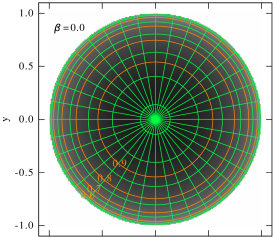
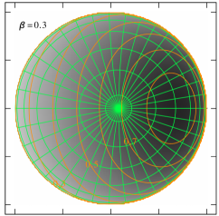
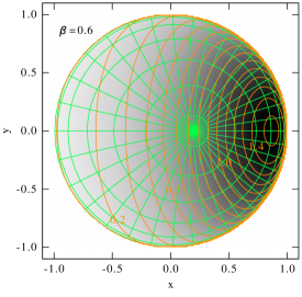
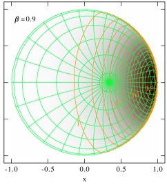
Figure 31: Radiance distribution of the Sun as seen from a moving observer. The radiance in the Sun’s rest frame includes limb darkening as in (3.4). The position and velocity direction of the observer is the same as in Fig. 29 except that $\beta$ is varied as indicated. The radiance is shown in reverse grey scale with contours superposed in orange. The maximum radiance values are 1.0, 0.8581, 1.5271, 16.2358 for the values of $\beta=$ 0, 0.3, 0.6 and 0.9, respectively. We have also superposed the spherical grid (green) with the pole pointing to the observer in rest frame of the sphere in as in Fig. 29. The grid appears less distorted than the radiance distribution.

The distortion of the visible surface of the sphere has consequences for distribution of the surface radiance. Compared to the rest frame, the radiance is enhanced inversely proportional to the area ratio of the surface grid elements between rest frame and moving frame as, e.g., shown in in the lower diagram of Fig. 29 [see also Kraus, 2000]. This apparent distortion of the sphere’s surface is expressed in the transformation of a space angular element $d\Omega^{\prime}/d\Omega=D^{2}(\mathbfl{\hat{k}},\boldsymbol{\beta})$ (D.27). In addition, the photon electric field is also transformed so that apparent surface radiance effectively transforms to the moving frame as in (D.29). As a result, the apparent radiance distribution in the moving frame is even more shifted to the forward hemisphere compared to the observer pole and its maximum value becomes for our geometry drastically enhanced for $\beta>0.4$. Recall that distortion of the visible surface not only increases with increasing $\beta$ but also with decreasing distance $r$ to the sphere.

D.8 Derivation of (5.24)

In this chapter we prove (5.24) using the definitions (5.13) to (5.22) for the two orthogonal polarisation $\mathbfl{\hat{p}}_{1}$ and $\mathbfl{\hat{p}}_{2}$.

We insert the definitions (5.14), (5.15) and (5.16) to obtain for $i=1$

$$\mathbfl{\hat{p}}_{1}^{\mathsf{T}}\mathbfl{\hat{k}}_{\mathrm{in}}=\sin\psi_{\mathrm{in}}\boldsymbol{\hat{\nu}}_{\mathrm{sc}}^{\mathsf{T}}\boldsymbol{\hat{\mu}}_{\mathrm{in}},\qquad\mathbfl{\hat{p}}^{\prime}{{}^{\mathsf{T}}_{1}}\mathbfl{\hat{k}}^{\prime}_{\mathrm{in}}=\sin\psi^{\prime}_{\mathrm{in}}\boldsymbol{\hat{\nu}}_{\mathrm{sc}}^{\mathsf{T}}\boldsymbol{\hat{\mu}}_{\mathrm{in}}$$

since $\boldsymbol{\hat{\nu}}_{\mathrm{sc}}\perp\boldsymbol{\hat{\beta}}$. The ratio between $\sin\psi^{\prime}_{\mathrm{in}}$ and $\sin\psi_{\mathrm{in}}$ is given by the aberration relation (D.12). Using definition (D.16), we have

$$\mathbfl{\hat{p}}^{\prime}{{}^{\mathsf{T}}_{1}}\mathbfl{\hat{k}}^{\prime}_{\mathrm{in}}=\sin\psi^{\prime}_{\mathrm{in}}\boldsymbol{\hat{\nu}}_{\mathrm{sc}}^{\mathsf{T}}\boldsymbol{\hat{\mu}}_{\mathrm{in}}=\frac{\sin\psi_{\mathrm{in}}}{\gamma(1-\beta\cos\psi_{\mathrm{in}})}\boldsymbol{\hat{\nu}}_{\mathrm{sc}}^{\mathsf{T}}\boldsymbol{\hat{\mu}}_{\mathrm{in}}=D(\mathbfl{\hat{k}}_{\mathrm{in}},\boldsymbol{\beta})\;\mathbfl{\hat{p}}^{\mathsf{T}}_{1}\mathbfl{\hat{k}}_{\mathrm{in}}$$

This relation is in agreement with (5.24) because $\mathbfl{\hat{p}}_{1}=\mathbfl{\hat{p}}^{\prime}_{1}=\boldsymbol{\hat{\nu}}_{\mathrm{sc}}$ is perpendicular to $\boldsymbol{\hat{\beta}}$.

For $i=2$ the derivation is somewhat more involved because $\mathbfl{\hat{p}}_{2}$ is not perpendicular $\boldsymbol{\hat{\beta}}$. We again insert (5.14), (5.15) and (5.16) and replace the aberrated angles by (D.11) and (D.12).

$$\mathbfl{\hat{p}}_{2}^{\mathsf{T}}\mathbfl{\hat{k}}_{\mathrm{in}}=\sin\psi_{\mathrm{in}}\cos\psi_{\mathrm{sc}}\boldsymbol{\hat{\mu}}_{\mathrm{in}}^{\mathsf{T}}\boldsymbol{\hat{\mu}}_{\mathrm{sc}}-\sin\psi_{\mathrm{sc}}\cos\psi_{\mathrm{in}}$$ (D.43)

$$\mathbfl{\hat{p}}^{\prime}{{}_{2}^{\mathsf{T}}}\mathbfl{\hat{k}}^{\prime}_{\mathrm{in}}=(\frac{\cos\psi_{\mathrm{in}}-\beta}{1-\beta\cos\psi_{\mathrm{in}}}\boldsymbol{\hat{\beta}}+\frac{\gamma^{-1}\sin\psi_{\mathrm{in}}}{1-\beta\cos\psi_{\mathrm{in}}}\boldsymbol{\hat{\mu}}_{\mathrm{in}})^{\mathsf{T}}(\frac{\cos\psi_{\mathrm{sc}}-\beta}{1-\beta\cos\psi_{\mathrm{sc}}}\boldsymbol{\hat{\mu}}_{\mathrm{sc}}-\frac{\gamma^{-1}\sin\psi_{\mathrm{sc}}}{1-\beta\cos\psi_{\mathrm{sc}}}\boldsymbol{\hat{\beta}})$$

$$\stackrel{{\scriptstyle\boldsymbol{\hat{\mu}}^{\mathsf{T}}\boldsymbol{\hat{\beta}}=0}}{{=}}\;\;\frac{\sin\psi_{\mathrm{in}}(\cos\psi_{\mathrm{sc}}-\beta)\boldsymbol{\hat{\mu}}_{\mathrm{in}}^{\mathsf{T}}\boldsymbol{\hat{\mu}}_{\mathrm{sc}}-\sin\psi_{\mathrm{sc}}(\cos\psi_{\mathrm{in}}-\beta)}{\gamma(1-\beta\cos\psi_{\mathrm{sc}})(1-\beta\cos\psi_{\mathrm{in}})}$$

$$=\frac{\sin\psi_{\mathrm{in}}\cos\psi_{\mathrm{sc}}\boldsymbol{\hat{\mu}}_{\mathrm{in}}^{\mathsf{T}}\boldsymbol{\hat{\mu}}_{\mathrm{sc}}-\sin\psi_{\mathrm{sc}}\cos\psi_{\mathrm{in}}-\beta\sin\psi_{\mathrm{in}}\boldsymbol{\hat{\mu}}_{\mathrm{in}}^{\mathsf{T}}\boldsymbol{\hat{\mu}}_{\mathrm{sc}}+\sin\psi_{\mathrm{sc}}\beta}{\gamma(1-\beta\cos\psi_{\mathrm{sc}})(1-\beta\cos\psi_{\mathrm{in}})}$$

$$\stackrel{{\scriptstyle\text{(}\ref{p2kin_0})}}{{=}}\frac{\mathbfl{\hat{p}}_{2}^{\mathsf{T}}\mathbfl{\hat{k}}_{\mathrm{in}}-\beta\sin\psi_{\mathrm{in}}\boldsymbol{\hat{\mu}}_{\mathrm{in}}^{\mathsf{T}}\boldsymbol{\hat{\mu}}_{\mathrm{sc}}+\sin\psi_{\mathrm{sc}}\beta}{\gamma(1-\beta\cos\psi_{\mathrm{sc}})(1-\beta\cos\psi_{\mathrm{in}})}$$

$$=\frac{\mathbfl{\hat{p}}_{2}^{\mathsf{T}}\mathbfl{\hat{k}}_{\mathrm{in}}}{\gamma(1-\beta\cos\psi_{\mathrm{in}})}+\frac{\mathbfl{\hat{p}}_{2}^{\mathsf{T}}\mathbfl{\hat{k}}_{\mathrm{in}}-\mathbfl{\hat{p}}_{2}^{\mathsf{T}}\mathbfl{\hat{k}}_{\mathrm{in}}(1-\beta\cos\psi_{\mathrm{sc}})-\beta\sin\psi_{\mathrm{in}}\boldsymbol{\hat{\mu}}_{\mathrm{in}}^{\mathsf{T}}\boldsymbol{\hat{\mu}}_{\mathrm{sc}}+\sin\psi_{\mathrm{sc}}\beta}{\gamma(1-\beta\cos\psi_{\mathrm{sc}})(1-\beta\cos\psi_{\mathrm{in}})}$$

$$=\frac{\mathbfl{\hat{p}}_{2}^{\mathsf{T}}\mathbfl{\hat{k}}_{\mathrm{in}}}{\gamma(1-\beta\cos\psi_{\mathrm{in}})}+\frac{\mathbfl{\hat{p}}_{2}^{\mathsf{T}}\mathbfl{\hat{k}}_{\mathrm{in}}\beta\cos\psi_{\mathrm{sc}}-\beta\sin\psi_{\mathrm{in}}\boldsymbol{\hat{\mu}}_{\mathrm{in}}^{\mathsf{T}}\boldsymbol{\hat{\mu}}_{\mathrm{sc}}+\sin\psi_{\mathrm{sc}}\beta}{\gamma(1-\beta\cos\psi_{\mathrm{sc}})(1-\beta\cos\psi_{\mathrm{in}})}$$

$$\stackrel{{\scriptstyle\text{(\ref{FrqDoppler})}}}{{=}}D(\mathbfl{\hat{k}}_{\mathrm{in}},\boldsymbol{\beta})\big{(}\mathbfl{\hat{p}}_{2}^{\mathsf{T}}\mathbfl{\hat{k}}_{\mathrm{in}}+\frac{\mathbfl{\hat{p}}_{2}^{\mathsf{T}}\mathbfl{\hat{k}}_{\mathrm{in}}\beta\cos\psi_{\mathrm{sc}}-\beta\sin\psi_{\mathrm{in}}\boldsymbol{\hat{\mu}}_{\mathrm{in}}^{\mathsf{T}}\boldsymbol{\hat{\mu}}_{\mathrm{sc}}+\sin\psi_{\mathrm{sc}}\beta}{1-\beta\cos\psi_{\mathrm{sc}}}\big{)}$$ (D.44)

In the last steps we have split off the first term in (5.24). The second term on the right-hand-side has already the correct denominator compared with (5.24) so that it only remains to analyse the numerator of the second term in (D.44). Inserting the expressions for $\mathbfl{\hat{p}}_{2}^{\mathsf{T}}\mathbfl{\hat{k}}_{\mathrm{in}}$ and $\boldsymbol{\hat{\mu}}_{\mathrm{in}}^{\mathsf{T}}\boldsymbol{\hat{\mu}}_{\mathrm{sc}}$ we find

$$\mathbfl{\hat{p}}_{2}^{\mathsf{T}}\mathbfl{\hat{k}}_{\mathrm{in}}\beta\cos\psi_{\mathrm{sc}}-\beta\sin\psi_{\mathrm{in}}\boldsymbol{\hat{\mu}}_{\mathrm{in}}^{\mathsf{T}}\boldsymbol{\hat{\mu}}_{\mathrm{sc}}+\sin\psi_{\mathrm{sc}}\beta$$

$$\stackrel{{\scriptstyle\text{(\ref{p2kin_0})}}}{{=}}(\sin\psi_{\mathrm{in}}\cos\psi_{\mathrm{sc}}\boldsymbol{\hat{\mu}}_{\mathrm{in}}^{\mathsf{T}}\boldsymbol{\hat{\mu}}_{\mathrm{sc}}-\sin\psi_{\mathrm{sc}}\cos\psi_{\mathrm{in}})\beta\cos\psi_{\mathrm{sc}}-\beta\sin\psi_{\mathrm{in}}\boldsymbol{\hat{\mu}}_{\mathrm{in}}^{\mathsf{T}}\boldsymbol{\hat{\mu}}_{\mathrm{sc}}+\sin\psi_{\mathrm{sc}}\beta$$

$$=\sin\psi_{\mathrm{in}}\cos\psi_{\mathrm{sc}}\boldsymbol{\hat{\mu}}_{\mathrm{in}}^{\mathsf{T}}\boldsymbol{\hat{\mu}}_{\mathrm{sc}}\beta\cos\psi_{\mathrm{sc}}-\sin\psi_{\mathrm{sc}}\cos\psi_{\mathrm{in}}\beta\cos\psi_{\mathrm{sc}}-\beta\sin\psi_{\mathrm{in}}\boldsymbol{\hat{\mu}}_{\mathrm{in}}^{\mathsf{T}}\boldsymbol{\hat{\mu}}_{\mathrm{sc}}+\sin\psi_{\mathrm{sc}}\beta$$

$$=\beta\sin\psi_{\mathrm{in}}(\cos^{2}\psi_{\mathrm{sc}}-1)\boldsymbol{\hat{\mu}}_{\mathrm{in}}^{\mathsf{T}}\boldsymbol{\hat{\mu}}+\beta\sin\psi_{\mathrm{sc}}(1-\cos\psi_{\mathrm{in}}\cos\psi_{\mathrm{sc}})$$

$$\stackrel{{\scriptstyle\text{(\ref{Aberr_mumu})}}}{{=}}-\beta\frac{\sin\psi_{\mathrm{in}}\sin^{2}\psi_{\mathrm{sc}}}{\sin\psi_{\mathrm{in}}\sin\psi_{\mathrm{sc}}}\mathbfl{\hat{k}}_{\mathrm{in}}^{\mathsf{T}}(\boldsymbol{1}-\boldsymbol{\hat{\beta}}\boldsymbol{\hat{\beta}}{}^{\mathsf{T}})\mathbfl{\hat{k}}_{\mathrm{sc}}+\beta\sin\psi_{\mathrm{sc}}(1-\cos\psi_{\mathrm{in}}\cos\psi_{\mathrm{sc}})$$

$$=-\beta\sin\psi_{\mathrm{sc}}(\cos\chi-\cos\psi_{\mathrm{in}}\cos\psi_{\mathrm{sc}})+\beta\sin\psi_{\mathrm{sc}}(1-\cos\psi_{\mathrm{in}}\cos\psi_{\mathrm{sc}})$$

$$=\beta\sin\psi_{\mathrm{sc}}(1-\cos\chi)\stackrel{{\scriptstyle\text{(\ref{PolBase})}}}{{=}}-(1-\cos\chi)\mathbfl{\hat{p}}_{2}^{\mathsf{T}}\boldsymbol{\hat{\beta}}$$

Inserting the numerator in (D.44) we obtain (5.24)

$$\mathbfl{\hat{p}}^{\prime}{{}_{2}^{\mathsf{T}}}\mathbfl{\hat{k}}^{\prime}_{\mathrm{in}}=D(\mathbfl{\hat{k}}_{\mathrm{in}},\boldsymbol{\beta})\big{(}\mathbfl{\hat{p}}_{2}^{\mathsf{T}}\mathbfl{\hat{k}}_{\mathrm{in}}-\frac{1-\cos\chi}{1-\beta\cos\psi_{\mathrm{sc}}}\mathbfl{\hat{p}}_{2}^{\mathsf{T}}\boldsymbol{\hat{\beta}}\big{)}$$

Appendix E Alternative derivation of the scattered radiant intensity

This derivation follows the approach used in the plasma physics and plasma diagnostics literature [e.g., Segre and Zanza, 2000, Hutchinson, 2002]. It does not use any transformations but rests entirely in the observer frame. The setup used in lab experiments differs largely from the situation of Thomson scattering in the corona. In particular, an unpolarised incident beam is not used in the lab and is not treated in related scattering calculations I am aware of.

E.1 Lienard-Wiechert potential

We start with the electromagnetic potential of an accelerated electron with orbit $\mathbfl{r}(t)$ which passes the site of the scattering which we called $\mathbfl{r}$ in the main text at the retarded time $t_{\mathrm{ret}}$. The coordinates $(t,\mathbfl{x})$ denote time and location at which the scattered field is observed. All times and coordinates are in the observer frame, the dash in this chapter just marks integration variables. The potential is [e.g., Jackson, 1998]

$$\phi(t,\mathbfl{x})=\frac{e}{4\pi\epsilon_{0}}\int_{-\infty}^{t}dt^{\prime}\frac{1}{|\mathbfl{x}-\mathbfl{r}(t^{\prime})|}\delta(t-t^{\prime}-\frac{|\mathbfl{x}-\mathbfl{r}(t^{\prime})|}{c})$$

$$\mathbfl{A}(t,\mathbfl{x})=\frac{e\mu_{0}}{4\pi}\int_{-\infty}^{t}dt^{\prime}\frac{\mathbfl{v}(t^{\prime})}{|\mathbfl{x}-\mathbfl{r}(t^{\prime})|}\delta(t-t^{\prime}-\frac{|\mathbfl{x}-\mathbfl{r}(t^{\prime})|}{c})$$

By the $\delta$ function integration, we can treat $t^{\prime}$ as an ordinary variable and move the evaluation of the retarded time to the final evaluation of the integral. The retarded time is only given implicitly by the intersection of the particle world line $(ct^{\prime},\mathbfl{r}(t^{\prime}))$with the backwards light cone $c(t^{\prime}-t)-|\mathbfl{x}-\mathbfl{r}(t^{\prime})|=0$ from the observation event at $(ct,\mathbfl{x})$. Formally, it is the solution for $t^{\prime}$ of $t^{\prime}=t-|\mathbfl{x}-\mathbfl{r}(t^{\prime})|/c$ . By $\boldsymbol{\beta}=\dot{\mathbfl{r}}/c$ we again denote the particle velocity. To keep the formulas short, we introduce some abbreviations

$$\boldsymbol{\ell}(t^{\prime},\mathbfl{x}) =\mathbfl{x}-\mathbfl{r}(t^{\prime})$$ distance vector from emitting particle to observer

$$\beta_{\ell}(t^{\prime}) =\boldsymbol{\beta}(t^{\prime})^{\mathsf{T}}\boldsymbol{\hat{\ell}}(t^{\prime}) \boldsymbol{\beta} \boldsymbol{\ell}$$ projection of along the direction of

$$T(t^{\prime},\mathbfl{x}) =|\mathbfl{x}-\mathbfl{r}(t^{\prime})|/c$$ travel time

$$\vartheta(t^{\prime},t,\mathbfl{x}) =t-t^{\prime}-T(t^{\prime},\mathbfl{x}) \delta$$ -function argument

$$t_{\mathrm{ret}}\quad \;\;|\quad\vartheta(t_{\mathrm{ret}},t,\mathbfl{x})=0$$ retarded time

With $\mu_{0}=1/c^{2}\epsilon_{0}$ and the above abbreviations we can write the potential concisely as

$$\frac{\phi}{c}(t,\mathbfl{x})=\frac{e}{4\pi\epsilon_{0}c^{2}}\int_{-\infty}^{t}dt^{\prime}\frac{1}{T(t^{\prime},\mathbfl{x})}\delta(\vartheta(t^{\prime},t,\mathbfl{x}))$$

$$\mathbfl{A}(t,\mathbfl{x})=\frac{e}{4\pi\epsilon_{0}c^{2}}\int_{-\infty}^{t}dt^{\prime}\frac{\boldsymbol{\beta}(t^{\prime})}{T(t^{\prime},\mathbfl{x})}\delta(\vartheta(t^{\prime},t,\mathbfl{x}))$$

To derive the wave field of the moving charge we have to differentiate with respect to $\mathbfl{x}$ and $t$. Later we will also have to differentiate with respect to $t^{\prime}$. The dependence on these arguments is made clear above by listing all arguments explicitly. Here a list of partial derivatives we will need

$$\partial_{t^{\prime}}\,T(t^{\prime},\mathbfl{x})= \partial_{t^{\prime}}\,\frac{|\mathbfl{x}-\mathbfl{r}(t^{\prime})|}{c}=-\frac{(\mathbfl{x}-\mathbfl{r}(t^{\prime}))^{\mathsf{T}}}{|\mathbfl{x}-\mathbfl{r}(t^{\prime})|}\frac{\mathbfl{\dot{r}}(t^{\prime})}{c}$$

$$= -\boldsymbol{\hat{\ell}}{}^{\mathsf{T}}(t^{\prime})\boldsymbol{\beta}(t^{\prime})=-\beta_{\ell}(t^{\prime})$$ (E.1)

$$c\boldsymbol{\nabla}{x}T(t^{\prime},\mathbfl{x})= \boldsymbol{\nabla}{x}|\mathbfl{x}-\mathbfl{r}(t^{\prime})|=\frac{\mathbfl{x}-\mathbfl{r}(t^{\prime})}{|\mathbfl{x}-\mathbfl{r}(t^{\prime})|}=\boldsymbol{\hat{\ell}}(t^{\prime},\mathbfl{x})$$ (E.2)

$$c\boldsymbol{\nabla}{x}\frac{1}{T(t^{\prime},\mathbfl{x})}= c^{2}\boldsymbol{\nabla}{x}\frac{1}{|\mathbfl{x}-\mathbfl{r}(t^{\prime})|}=-c^{2}\frac{\mathbfl{x}-\mathbfl{r}(t^{\prime})}{|\mathbfl{x}-\mathbfl{r}(t^{\prime})|^{3}}=-\frac{\boldsymbol{\hat{\ell}}(t^{\prime},\mathbfl{x})}{T^{2}(t^{\prime},\mathbfl{x})}$$ (E.3)

$$\partial_{t}\,\vartheta(t^{\prime},t,\mathbfl{x})= \partial_{t}\,\!(t-t^{\prime}-T(t^{\prime},\mathbfl{x}))=1$$ (E.4)

$$\partial_{t^{\prime}}\,\vartheta(t^{\prime},t,\mathbfl{x})= \partial_{t^{\prime}}\,\!(t-t^{\prime}-T(t^{\prime},\mathbfl{x}))=-1-\partial_{t^{\prime}}\,T(t^{\prime},\mathbfl{x})$$ (E.5)

$$= -1+\boldsymbol{\hat{\ell}}{}^{\mathsf{T}}(t^{\prime})\boldsymbol{\beta}(t^{\prime})=-(1-\beta_{\ell}(t^{\prime}))=-\kappa(t^{\prime})$$ (E.6)

$$c\boldsymbol{\nabla}{x}\vartheta(t^{\prime},t,\mathbfl{x})= c\boldsymbol{\nabla}{x}(t-t^{\prime}-T(t^{\prime},\mathbfl{x}))=-c\boldsymbol{\nabla}{x}T(t^{\prime},\mathbfl{x})=-\boldsymbol{\hat{\ell}}(t^{\prime},\mathbfl{x})$$ (E.7)

With these rules the electric field becomes

$$\mathbfl{E}(t,\mathbfl{x})=-c\boldsymbol{\nabla}{x}\frac{\phi}{c}-\partial_{t}\,\!\mathbfl{A}$$

$$\stackrel{{\scriptstyle\text{(\ref{grd_invT})}}}{{=}}\frac{e}{4\pi\epsilon_{0}c^{2}}\int_{-\infty}^{t}dt^{\prime}\big{[}\frac{\boldsymbol{\hat{\ell}}(t^{\prime},\mathbfl{x})}{T^{2}(t^{\prime},\mathbfl{x})}\;\delta(\vartheta(t,\mathbfl{x},t^{\prime}))-\frac{1}{T(t^{\prime},\mathbfl{x})}\,c\boldsymbol{\nabla}{x}\delta(\vartheta(t,\mathbfl{x},t^{\prime}))$$

$$-\frac{\boldsymbol{\beta}(t^{\prime})}{T(t^{\prime},\mathbfl{x})}\partial_{t}\,\delta(\vartheta(t,\mathbfl{x},t^{\prime}))\big{]}$$

$$=\frac{e}{4\pi\epsilon_{0}c^{2}}\int_{-\infty}^{t}dt^{\prime}\big{[}\frac{\boldsymbol{\hat{\ell}}(t^{\prime},\mathbfl{x})}{T^{2}(t^{\prime},\mathbfl{x})}\;\delta(\vartheta(t,\mathbfl{x},t^{\prime}))-\frac{\delta^{\prime}(\vartheta(t,\mathbfl{x},t^{\prime}))}{T(t^{\prime},\mathbfl{x})}(c\boldsymbol{\nabla}{x}+\boldsymbol{\beta}(t^{\prime})\partial_{t}\,)\vartheta(t,\mathbfl{x},t^{\prime})\big{]}$$

$$\stackrel{{\scriptstyle\text{(\ref{dt_vartheta},\ref{grd_vartheta})}}}{{=}}\frac{e}{4\pi\epsilon_{0}c^{2}}\int_{-\infty}^{t}dt^{\prime}\big{[}\frac{\boldsymbol{\hat{\ell}}(t^{\prime},\mathbfl{x})}{T^{2}(t^{\prime},\mathbfl{x})}\;\delta(\vartheta(t,\mathbfl{x},t^{\prime}))-\frac{\delta^{\prime}(\vartheta(t,\mathbfl{x},t^{\prime}))}{T(t^{\prime},\mathbfl{x})}(-\boldsymbol{\hat{\ell}}(t^{\prime},\mathbfl{x})+\boldsymbol{\beta}(t^{\prime}))\big{]}$$

$$=\frac{e}{4\pi\epsilon_{0}c^{2}}\int_{-\infty}^{t}dt^{\prime}\big{[}\frac{\boldsymbol{\hat{\ell}}(t^{\prime},\mathbfl{x})}{T^{2}(t^{\prime},\mathbfl{x})}\;\delta(\vartheta(t,\mathbfl{x},t^{\prime}))+\frac{\boldsymbol{\hat{\ell}}(t^{\prime},\mathbfl{x})-\boldsymbol{\beta}(t^{\prime})}{T(t^{\prime},\mathbfl{x})}\delta^{\prime}(\vartheta(t,\mathbfl{x},t^{\prime}))\big{]}$$

Next we replace the integration variable $t^{\prime}$ by $\vartheta(t,\mathbfl{x},t^{\prime})$. Then the particle time $t^{\prime}$ becomes a function of $t,\mathbfl{x}$ and $\vartheta$. The Jacobian of this transformation has the inverse magnitude of $|\partial_{t^{\prime}}\,\vartheta(t,\mathbfl{x},t^{\prime})|=|\kappa(t^{\prime},\mathbfl{x})|$, see (E.4). Note that since $\beta_{\ell}\leq\beta<1$, $\kappa=1-\beta_{\ell}$ is always positive. We can therefore substitute $dt^{\prime}=|\kappa|^{-1}\;d\vartheta=\kappa^{-1}\;d\vartheta$. The old integration boundaries $t^{\prime}=-\infty\dots t$ map to $\vartheta=-T(t,\mathbfl{x})\dots\infty$. Since $T>0$ the $\delta$-function gives exactly one contribution at $\vartheta=0$ and the lower boundary does not really matter. We can replace it by $-\infty$.

$$\mathbfl{E}(t,\mathbfl{x})=\frac{e}{4\pi\epsilon_{0}c^{2}}\int_{-\infty}^{\infty}\frac{d\vartheta}{\kappa(t^{\prime}(\vartheta),\mathbfl{x})}\big{[}\frac{\boldsymbol{\hat{\ell}}(t^{\prime}(\vartheta),\mathbfl{x})}{T^{2}(t^{\prime}(\vartheta),\mathbfl{x})}\delta(\vartheta)+\frac{\boldsymbol{\hat{\ell}}(t^{\prime}(\vartheta),\mathbfl{x})-\boldsymbol{\beta}(t^{\prime}(\vartheta))}{T(t^{\prime}(\vartheta),\mathbfl{x})}\delta^{\prime}(\vartheta)\big{]}$$

Next we partially integrate the 2nd term to get rid of the derivative of the $\delta$ function and change the derivative with respect to $\vartheta$ back to a derivative with respect to $t^{\prime}$:

$$\int d\vartheta\;[\frac{\boldsymbol{\hat{\ell}}-\boldsymbol{\beta}}{\kappa T}]\;\frac{d\delta}{d\vartheta}=-\int d\vartheta\;\delta\;\frac{d}{d\vartheta}[\frac{\boldsymbol{\hat{\ell}}-\boldsymbol{\beta}}{\kappa T}]=-\int d\vartheta\;\delta\;\frac{1}{(-\kappa)}\frac{d}{dt^{\prime}}[\frac{\boldsymbol{\hat{\ell}}-\boldsymbol{\beta}}{\kappa T}]$$

Gives

$$\mathbfl{E}(t,\mathbfl{x})=\frac{e}{4\pi\epsilon_{0}c^{2}}\int_{-\infty}^{\infty}d\vartheta\frac{\delta(\vartheta)}{\kappa(t^{\prime}(\vartheta),\mathbfl{x})}\big{[}\frac{\boldsymbol{\hat{\ell}}(t^{\prime}(\vartheta),\mathbfl{x})}{T^{2}(t^{\prime}(\vartheta),\mathbfl{x})}+\frac{d}{dt^{\prime}}\big{(}\frac{\boldsymbol{\hat{\ell}}(t^{\prime},\mathbfl{x})-\boldsymbol{\beta}(t^{\prime})}{\kappa(t^{\prime},\mathbfl{x})T(t^{\prime},\mathbfl{x})}\big{)}_{t^{\prime}=t^{\prime}(\vartheta)}\big{]}$$ (E.8)

For the derivative with respect to $t^{\prime}$ in (E.8) we use (E.1) and (E.4) and (omitting the arguments)

$$\frac{d}{dt^{\prime}}\boldsymbol{\beta}=\boldsymbol{\dot{\beta}}\qquad\frac{d}{dt^{\prime}}\boldsymbol{\ell}=\frac{d}{dt^{\prime}}(\mathbfl{x}-\mathbfl{r})=-c\boldsymbol{\beta}$$

$$\frac{d}{dt^{\prime}}\frac{1}{T}=-\frac{1}{T^{2}}\frac{d}{dt^{\prime}}T\stackrel{{\scriptstyle\text{(\ref{dtd_T})}}}{{=}}\frac{1}{T^{2}}\beta_{\ell}$$

$$\frac{d}{dt^{\prime}}\boldsymbol{\hat{\ell}}=\frac{d}{dt^{\prime}}\frac{\boldsymbol{\ell}}{\ell}=-\frac{1}{T}\boldsymbol{\beta}+\frac{\boldsymbol{\ell}}{c}\;\frac{d}{dt^{\prime}}\frac{1}{T}=-\frac{1}{T}\boldsymbol{\beta}+\frac{\boldsymbol{\ell}}{c}\;\frac{\beta_{\ell}}{T^{2}}=-\frac{1}{T}\boldsymbol{\beta}+\boldsymbol{\hat{\ell}}\;\frac{1}{T}\beta_{\ell}$$

$$=\frac{1}{T}(\beta_{\ell}\boldsymbol{\hat{\ell}}-\boldsymbol{\beta})=-\frac{1}{T}(\boldsymbol{1}-\boldsymbol{\hat{\ell}}\boldsymbol{\hat{\ell}}{}^{\mathsf{T}})\boldsymbol{\beta}$$

$$\frac{d}{dt^{\prime}}\kappa=\frac{d}{dt^{\prime}}(1-\beta_{\ell})=-\frac{d}{dt^{\prime}}\boldsymbol{\hat{\ell}}{}^{\mathsf{T}}\boldsymbol{\beta}=-\boldsymbol{\hat{\ell}}{}^{\mathsf{T}}\boldsymbol{\dot{\beta}}+\frac{1}{T}\boldsymbol{\beta}^{\mathsf{T}}(1-\boldsymbol{\hat{\ell}}\boldsymbol{\hat{\ell}}{}^{\mathsf{T}})\boldsymbol{\beta}=-\dot{\beta}_{\ell}+\frac{1}{T}(\beta^{2}-\beta_{\ell}^{2})$$

$$\frac{d}{dt^{\prime}}\frac{1}{\kappa}=-\frac{1}{\kappa^{2}}\frac{d}{dt^{\prime}}\kappa=\frac{1}{\kappa^{2}}(\dot{\beta}_{\ell}+\frac{1}{T}(\beta_{\ell}^{2}-\beta^{2}))$$

The square bracket in the integrand of (E.8) then gives

$$\frac{\boldsymbol{\hat{\ell}}}{T^{2}}+\frac{d}{dt^{\prime}}\frac{\boldsymbol{\hat{\ell}}-\boldsymbol{\beta}}{\kappa\,T}$$

$$=\underbrace{\frac{\kappa^{2}\boldsymbol{\hat{\ell}}}{\kappa^{2}T^{2}}}_{\text{1}}+\frac{1}{\kappa T}[\underbrace{\frac{\beta_{\ell}\boldsymbol{\hat{\ell}}-\boldsymbol{\beta}}{T}}_{\text{2}}-\underbrace{\boldsymbol{\dot{\beta}}}_{\text{3}}]+\underbrace{\frac{\boldsymbol{\hat{\ell}}-\boldsymbol{\beta}}{\kappa}\,\frac{\beta_{\ell}}{T^{2}}}_{\text{4}}+\frac{\boldsymbol{\hat{\ell}}-\boldsymbol{\beta}}{T}\,\frac{1}{\kappa^{2}}(\underbrace{\dot{\beta}_{\ell}}_{\text{5}}+\underbrace{\frac{1}{T}(\beta_{\ell}^{2}-\beta^{2})}_{\text{6}})$$

We first order the terms according to powers of $T^{-1}$ and secondly according to the vector coefficient

$$\frac{\boldsymbol{\hat{\ell}}}{T^{2}}+\frac{d}{dt^{\prime}}\frac{\boldsymbol{\hat{\ell}}-\boldsymbol{\beta}}{\kappa\,T}=\frac{1}{\kappa^{2}T}[-\overbrace{\kappa\boldsymbol{\dot{\beta}}}^{3}+\overbrace{(\boldsymbol{\hat{\ell}}-\boldsymbol{\beta})\dot{\beta}_{\ell}}^{5}]$$

$$+\frac{1}{\kappa^{2}T^{2}}[\overbrace{\kappa^{2}\boldsymbol{\hat{\ell}}}^{1}+\overbrace{\kappa(\beta_{\ell}\boldsymbol{\hat{\ell}}-\boldsymbol{\beta})}^{2}+\overbrace{\kappa(\boldsymbol{\hat{\ell}}-\boldsymbol{\beta})\beta_{\ell}}^{4}+\overbrace{(\boldsymbol{\hat{\ell}}-\boldsymbol{\beta})(\beta_{\ell}^{2}-\beta^{2})}^{6}]$$

$$\text{term}\propto\frac{1}{\kappa^{2}T}:\qquad-\kappa\boldsymbol{\dot{\beta}}+(\boldsymbol{\hat{\ell}}-\boldsymbol{\beta})\dot{\beta}_{\ell}=(\boldsymbol{\hat{\ell}}-\boldsymbol{\beta})\dot{\beta}_{\ell}-(1-\beta_{\ell})\boldsymbol{\dot{\beta}}$$

$$=(\boldsymbol{\hat{\ell}}-\boldsymbol{\beta})\boldsymbol{\hat{\ell}}{}^{\mathsf{T}}\boldsymbol{\dot{\beta}}-\boldsymbol{\hat{\ell}}{}^{\mathsf{T}}(\boldsymbol{\hat{\ell}}-\mathbfl{\beta})\boldsymbol{\dot{\beta}}=\boldsymbol{\hat{\ell}}\times(\boldsymbol{\hat{\ell}}-\boldsymbol{\beta})\times\boldsymbol{\dot{\beta}}$$

$$\text{term}\propto\frac{1}{\kappa^{2}T^{2}}:\qquad\kappa^{2}\boldsymbol{\hat{\ell}}+\kappa(\beta_{\ell}\boldsymbol{\hat{\ell}}-\boldsymbol{\beta})+\kappa(\boldsymbol{\hat{\ell}}-\boldsymbol{\beta})\beta_{\ell}+(\boldsymbol{\hat{\ell}}-\boldsymbol{\beta})(\beta_{\ell}^{2}-\beta^{2})$$

$$=(\kappa^{2}+2\kappa\beta_{\ell}+\beta_{\ell}^{2}-\beta^{2})\boldsymbol{\hat{\ell}}-(\kappa+\kappa\beta_{\ell}+\beta^{2}_{\ell}-\beta^{2})\boldsymbol{\beta}$$

$$=((\kappa+\beta_{\ell})^{2}-\beta^{2})\boldsymbol{\hat{\ell}}-(\kappa(1+\beta_{\ell})+\beta^{2}_{\ell}-\beta^{2})\boldsymbol{\beta}$$

$$=(1-\beta^{2})\boldsymbol{\hat{\ell}}-(1-\beta_{\ell}^{2}+\beta^{2}_{\ell}-\beta^{2})\boldsymbol{\beta}$$

$$=(1-\beta^{2})\boldsymbol{\hat{\ell}}-(1-\beta^{2})\boldsymbol{\beta}=\frac{1}{\gamma^{2}}(\boldsymbol{\hat{\ell}}-\boldsymbol{\beta})$$

Inserting the two final terms for the square bracket of (E.8), we find

$$\mathbfl{E}(t,\mathbfl{x})=\frac{e}{4\pi\epsilon_{0}c^{2}}\int_{-\infty}^{\infty}\frac{d\vartheta}{\kappa^{3}}\big{[}\frac{\boldsymbol{\hat{\ell}}\times(\boldsymbol{\hat{\ell}}-\boldsymbol{\beta})\times\boldsymbol{\dot{\beta}}}{T}+\frac{\boldsymbol{\hat{\ell}}-\boldsymbol{\beta}}{\gamma^{2}T^{2}}\big{]}\delta(\vartheta)$$

where $\delta(\vartheta)$ fixes $t^{\prime}$ to the retarded time $t_{\mathrm{ret}}$. Since the retarded time can be explicitly calculated only in few cases we can execute the integration only symbolically by writing

$$\mathbfl{E}(t,\mathbfl{x})=\frac{e}{4\pi\epsilon_{0}c^{2}}\big{[}\frac{\boldsymbol{\hat{\ell}}\times(\boldsymbol{\hat{\ell}}-\boldsymbol{\beta})\times\boldsymbol{\dot{\beta}}}{\kappa^{3}T}+\frac{\boldsymbol{\hat{\ell}}-\boldsymbol{\beta}}{\gamma^{2}\kappa^{3}T^{2}}\big{]}_{t_{\mathrm{ret}}}$$ (E.9)

The first term depends on the acceleration of the particle and is the radiative part of the field. It decreases with $T^{-1}=c/\ell$ from the retarded position of the particle. In the far field only this term is important. Obviously, the radiating part of the field is perpendicular to the retarded direction $\boldsymbol{\hat{\ell}}(t_{\mathrm{ret}})$ from the source. This part will be discussed further below as the source of the scattered wave field.

E.2 Electrostatic part

The second term in (E.9) is the electrostatic field component decreasing more rapidly with $T^{-2}=(c/\ell)^{2}$. The static field is largely longitudinal. For a particle with a constant, non-accelerated velocity this is the only term in (E.9). We assume the charged particle moves with constant $\mathbfl{v}=c\boldsymbol{\beta}$ along the trajectory $\mathbfl{r}(t)=\mathbfl{r}_{0}+\mathbfl{v}t$. Then the field observed at $(t,\mathbfl{x})$ is directed along

$$\boldsymbol{\hat{\ell}}(t_{\mathrm{ret}})-\boldsymbol{\beta}=\frac{\mathbfl{x}-\mathbfl{r}_{0}-\mathbfl{v}t_{\mathrm{ret}}}{\ell(t_{\mathrm{ret}})}-\frac{\mathbfl{v}}{c}=\frac{\mathbfl{x}-\mathbfl{r}_{0}-\mathbfl{v}t_{\mathrm{ret}}-\mathbfl{v}d(t_{\mathrm{ret}})/c}{\ell(t_{\mathrm{ret}})}$$

$$=\frac{\mathbfl{x}-\mathbfl{r}_{0}-\mathbfl{v}t_{\mathrm{ret}}-\mathbfl{v}T(t_{\mathrm{ret}})}{\ell(t_{\mathrm{ret}})}=\frac{\mathbfl{x}-\mathbfl{r}_{0}-\mathbfl{v}t}{\ell(t_{\mathrm{ret}})}=\frac{\boldsymbol{\ell}(t)}{\ell(t_{\mathrm{ret}})}$$

This has not the retarded but the actual direction from the source. The field therefore becomes

$$\mathbfl{E}_{\mathrm{stat}}(t,\mathbfl{x})=\frac{e}{4\pi\epsilon_{0}c^{2}}\big{[}\frac{\boldsymbol{\hat{\ell}}-\boldsymbol{\beta}}{\gamma^{2}\kappa^{3}T^{2}}\big{]}_{t_{\mathrm{ret}}}=\frac{e}{4\pi\epsilon_{0}}\frac{\boldsymbol{\ell}(t)}{\gamma^{2}\kappa^{3}\ell^{3}(t_{\mathrm{ret}})}$$ (E.10)

The denominator can be evaluated as follows: Be $d$ the minimum distance of the particle path from the observer at $\mathbfl{x}$ and the point $\mathbfl{r}_{0}$ of closest approach passed by the particle at $t=0$. Then [Rybicki and Lightman, 1979]

$$\boldsymbol{\ell}(t)=\mathbfl{x}-\mathbfl{r(t)}=(-vt,d)\quad\text{in a suitably rotated coordinate system.}$$

$$\text{Then}\quad\ell^{2}(t)=d^{2}+v^{2}t^{2}\quad\text{and}$$

$$\ell^{2}(t_{\mathrm{ret}})=d^{2}+v^{2}t_{\mathrm{ret}}^{2}=d^{2}+v^{2}(t-\frac{\ell(t_{\mathrm{ret}})}{c})^{2}=\ell^{2}(t)-2\beta vt\;\ell(t_{\mathrm{ret}})+\beta^{2}\ell^{2}(t_{\mathrm{ret}})$$

$$\text{give}\quad\ell^{2}(t_{\mathrm{ret}})+2\gamma^{2}\beta vt\;\ell(t_{\mathrm{ret}})-\gamma^{2}\ell^{2}(t)=0$$

$$\text{or}\quad\ell(t_{\mathrm{ret}})=-\gamma^{2}\beta vt+\sqrt{\rule{0.0pt}{8.61108pt}\gamma^{4}\beta v^{2}t^{2}+\gamma^{2}\ell^{2}(t)}=-\gamma^{2}\beta vt+\gamma\sqrt{\rule{0.0pt}{8.61108pt}(\gamma\beta vt)^{2}+\ell^{2}(t)}$$ (E.11)

$$\text{Next evaluate}\quad\gamma^{2}\kappa\ell(t_{\mathrm{ret}})=\gamma^{2}(\ell(t_{\mathrm{ret}})-\boldsymbol{\beta}^{\mathsf{T}}\boldsymbol{\ell}(r_{\mathrm{ret}}))=\gamma^{2}(\ell(t_{\mathrm{ret}})+\beta vt_{\mathrm{ret}})$$

$$=\gamma^{2}(\ell(t_{\mathrm{ret}})+\beta v(t-\frac{\ell(t_{\mathrm{ret}})}{c}))=\gamma^{2}(\ell(t_{\mathrm{ret}})+\beta vt-\beta^{2}\ell(t_{\mathrm{ret}}))=\ell(t_{\mathrm{ret}})+\gamma^{2}\beta vt$$ (E.12)

$$\text{compare (\ref{retdist}) and (\ref{kapparetdist})}\quad\gamma^{2}\kappa\ell(t_{\mathrm{ret}})=\gamma\sqrt{\rule{0.0pt}{8.61108pt}(\gamma\beta vt)^{2}+\ell^{2}(t)}$$

Insertion in (E.10) yields the electrostatic field in a form where the retarded time does not occur any more

$$\mathbfl{E}_{\mathrm{stat}}(t,\mathbfl{x})=\frac{e}{4\pi\epsilon_{0}}\frac{\gamma\boldsymbol{\ell}(t)}{\rule{0.0pt}{8.61108pt}((\gamma\beta vt)^{2}+\ell^{2}(t))^{3/2}}=\frac{e}{4\pi\epsilon_{0}}\frac{\gamma\boldsymbol{\ell}(t)}{\rule{0.0pt}{8.61108pt}((\gamma^{2}\beta^{2}+1)(vt)^{2}+d^{2})^{3/2}}$$

$$=\frac{e}{4\pi\epsilon_{0}}\frac{\gamma\boldsymbol{\ell}(t)}{\rule{0.0pt}{8.61108pt}((\gamma vt)^{2}+d^{2})^{3/2}}$$ (E.13)

E.3 Acceleration of a point charge in a wave field

For the radiating part of the field in (E.9) we specify the particle acceleration as being the result of an incident electromagnetic wave which propagates in direction $\mathbfl{\hat{k}}_{\mathrm{in}}$ and has the wave field $\mathbfl{E}_{\mathrm{in}}(t,\mathbfl{x})$ and $c\mathbfl{B}_{\mathrm{in}}(t,\mathbfl{x})=\mathbfl{\hat{k}}_{\mathrm{in}}\times\mathbfl{E}_{\mathrm{in}}(t,\mathbfl{x})$. Like above, we will also abbreviate the projection of $\boldsymbol{\beta}$ along $\mathbfl{\hat{k}}_{\mathrm{in}}$ by $\beta_{\mathrm{in}}=\boldsymbol{\beta}^{\mathsf{T}}\mathbfl{\hat{k}}_{\mathrm{in}}=\beta\cos\psi_{\mathrm{in}}$. The relativistic equation of motion of an electron with rest mass $m_{e}$ is [e.g., Jackson, 1998]

$$\frac{\partial}{\partial t}\mathbfl{p}=\frac{\partial}{\partial t}\gamma m_{e}\mathbfl{v}=-e(\mathbfl{E}_{\mathrm{in}}+\mathbfl{v}\times\mathbfl{B}_{\mathrm{in}})=-e(\mathbfl{E}_{\mathrm{in}}+\boldsymbol{\beta}\times c\mathbfl{B}_{\mathrm{in}})=-e[(1-\beta_{\mathrm{in}})\boldsymbol{1}+\mathbfl{\hat{k}}_{\mathrm{in}}\boldsymbol{\beta}^{\mathsf{T}}]\mathbfl{E}_{\mathrm{in}}$$

$$\text{or}\quad\frac{\partial}{\partial t}\gamma\boldsymbol{\beta}=-\frac{e}{m_{e}c}[(1-\beta_{\mathrm{in}})\boldsymbol{1}+\mathbfl{\hat{k}}_{\mathrm{in}}\boldsymbol{\beta}^{\mathsf{T}}]\mathbfl{E}_{\mathrm{in}}$$

$$\text{Using}\quad\frac{\partial}{\partial t}\gamma=\frac{\partial}{\partial t}\frac{1}{\sqrt{1-\beta^{2}}}=\frac{\boldsymbol{\beta}^{\mathsf{T}}\boldsymbol{\dot{\beta}}}{\sqrt{1-\beta^{2}}^{3}}=\gamma^{3}\boldsymbol{\beta}^{\mathsf{T}}\boldsymbol{\dot{\beta}}\quad\text{we find}$$

$$\frac{\partial}{\partial t}\gamma\boldsymbol{\beta}=\dot{\gamma}\boldsymbol{\beta}+\gamma\boldsymbol{\dot{\beta}}=\gamma^{3}\boldsymbol{\beta}\;\boldsymbol{\beta}^{\mathsf{T}}\boldsymbol{\dot{\beta}}+\gamma\boldsymbol{\dot{\beta}}=\gamma(\gamma^{2}\boldsymbol{\beta}\;\boldsymbol{\beta}^{\mathsf{T}}\boldsymbol{\dot{\beta}}+\boldsymbol{\dot{\beta}})$$

$$=-\frac{e}{m_{e}c}[(1-\beta_{\mathrm{in}})\boldsymbol{1}+\mathbfl{\hat{k}}_{\mathrm{in}}\boldsymbol{\beta}^{\mathsf{T}}]\mathbfl{E}_{\mathrm{in}}$$ (E.14)

We first solve for the projection along $\boldsymbol{\beta}$. A scalar multiplication of (E.14) with $\boldsymbol{\beta}$ yields

$$\gamma^{2}\beta^{2}\;\boldsymbol{\beta}^{\mathsf{T}}\boldsymbol{\dot{\beta}}+\boldsymbol{\beta}^{\mathsf{T}}\boldsymbol{\dot{\beta}}=(\gamma^{2}\beta^{2}+1)\boldsymbol{\beta}^{\mathsf{T}}\boldsymbol{\dot{\beta}}=\gamma^{2}\boldsymbol{\beta}^{\mathsf{T}}\boldsymbol{\dot{\beta}}=-\frac{e}{\gamma m_{e}c}\boldsymbol{\beta}^{\mathsf{T}}\mathbfl{E}_{\mathrm{in}}$$

Insertion of $\gamma^{2}\boldsymbol{\beta}^{\mathsf{T}}\boldsymbol{\dot{\beta}}$ in (E.14) gives

$$\boldsymbol{\dot{\beta}}=-\frac{e}{\gamma m_{e}c}[(1-\beta_{\mathrm{in}})\boldsymbol{1}+\mathbfl{\hat{k}}_{\mathrm{in}}\boldsymbol{\beta}^{\mathsf{T}}]\mathbfl{E}_{\mathrm{in}}-\gamma^{2}\boldsymbol{\beta}\;\boldsymbol{\beta}^{\mathsf{T}}\boldsymbol{\dot{\beta}}$$

$$=-\frac{e}{\gamma m_{e}c}[(1-\beta_{\mathrm{in}})\boldsymbol{1}+\mathbfl{\hat{k}}_{\mathrm{in}}\boldsymbol{\beta}^{\mathsf{T}}]\mathbfl{E}_{\mathrm{in}}+\frac{e}{\gamma m_{e}c}\boldsymbol{\beta}\;\boldsymbol{\beta}^{\mathsf{T}}\mathbfl{E}_{\mathrm{in}}$$

$$=-\frac{e}{\gamma m_{e}c}((1-\beta_{\mathrm{in}})\boldsymbol{1}+(\mathbfl{\hat{k}}_{\mathrm{in}}-\boldsymbol{\beta})\boldsymbol{\beta}^{\mathsf{T}}]\mathbfl{E}_{\mathrm{in}}$$ (E.15)

Hence the acceleration in the wave field is not just parallel to the electric field as in the non-relativistic case. There is also a component in the direction of wave propagation from the wave Lorentz force which transfers some momentum from the photon to the electron. There is also a breaking component along $-\boldsymbol{\beta}$ which prevents the velocity to exceed $\beta=1$.

E.4 Scattered wave field

For the scattering problem, only the radiative term in (E.9) counts where the acceleration $\boldsymbol{\dot{\beta}}$ is replaced by (E.15). The electric field (E.9) is then called $\mathbfl{E}_{\mathrm{sc}}$ and the direction $\boldsymbol{\hat{\ell}}$ corresponds to the propagation direction $\mathbfl{\hat{k}}_{\mathrm{sc}}$ of the scattered wave. Accordingly, $\beta_{\ell}$ will be renamed in $\beta_{\mathrm{sc}}=\boldsymbol{\beta}^{\mathsf{T}}\mathbfl{\hat{k}}_{\mathrm{sc}}=\beta\cos\psi_{\mathrm{sc}}$. Moreover, we abbreviate

$$\mathbfl{h}_{\mathrm{in}}=\mathbfl{\hat{k}}_{\mathrm{in}}-\boldsymbol{\beta},\qquad\mathbfl{h}_{\mathrm{sc}}=\mathbfl{\hat{k}}_{\mathrm{sc}}-\boldsymbol{\beta}$$

Note the vectors $\mathbfl{h}_{\mathrm{in}}$ and $\mathbfl{h}_{\mathrm{sc}}$ are not unit vectors any more. In particular

$$\mathbfl{h}_{\mathrm{sc}}^{\mathsf{T}}\mathbfl{\hat{k}}_{\mathrm{sc}}=1-\beta_{\mathrm{sc}},\qquad\mathbfl{h}_{\mathrm{sc}}^{\mathsf{T}}\mathbfl{\hat{k}}_{\mathrm{in}}=\cos\chi-\beta_{\mathrm{in}},\qquad\mathbfl{h}_{\mathrm{sc}}^{\mathsf{T}}\boldsymbol{\hat{\beta}}=\beta_{\mathrm{sc}}-\beta^{2}$$

$$\mathbfl{h}_{\mathrm{sc}}^{\mathsf{T}}\mathbfl{h}_{\mathrm{in}}=\cos\chi-\beta_{\mathrm{in}}-\beta_{\mathrm{sc}}+\beta^{2}$$

and similarly for “sc” replaced by ”in”. The angle $\chi=\mathrm{acos}\;\mathbfl{\hat{k}}_{\mathrm{sc}}^{\mathsf{T}}\mathbfl{\hat{k}}_{\mathrm{in}}$ is the scattering angle. Insertion of (E.15) into the radiation part of (E.9) we obtain

$$\mathbfl{E}_{\mathrm{sc}}(t,\mathbfl{x})=\frac{e}{4\pi\epsilon_{0}c^{2}}\big{[}\frac{\mathbfl{\hat{k}}_{\mathrm{sc}}\times\mathbfl{h}_{\mathrm{sc}}\times\boldsymbol{\dot{\beta}}}{\kappa^{3}T}\big{]}_{t_{\mathrm{ret}}}$$

$$=\frac{-e^{2}}{4\pi\epsilon_{0}m_{e}c^{2}}\big{[}\frac{\mathbfl{\hat{k}}_{\mathrm{sc}}\times\mathbfl{h}_{\mathrm{sc}}\times[(1-\beta_{\mathrm{in}})\mathbfl{E}_{\mathrm{in}}+\boldsymbol{\beta}^{\mathsf{T}}\mathbfl{E}_{\mathrm{in}}\;\mathbfl{h}_{\mathrm{in}}]}{\gamma\kappa^{3}cT}\big{]}_{t_{\mathrm{ret}}}$$

$$=-r_{e}\big{[}\frac{[(1-\beta_{\mathrm{sc}})\boldsymbol{1}-\mathbfl{h}_{\mathrm{sc}}\mathbfl{\hat{k}}_{\mathrm{sc}}^{\mathsf{T}}]\;[(1-\beta_{\mathrm{in}})\boldsymbol{1}+\mathbfl{h}_{\mathrm{in}}\boldsymbol{\beta}^{\mathsf{T}}]\;\mathbfl{E}_{\mathrm{in}}}{\gamma\kappa^{3}\ell}\big{]}_{t_{\mathrm{ret}}}=-r_{e}\big{[}\frac{\mathbfl{S}\mathbfl{A}\mathbfl{E}_{\mathrm{in}}}{\gamma\kappa^{3}\ell}\big{]}_{t_{\mathrm{ret}}}$$ (E.16)

where we used the classical electron radius $r_{e}=e^{2}/4\pi\epsilon_{0}m_{e}c^{2}$ and the distance $\ell=cT$ between the scattering site $\mathbfl{r}(t_{\mathrm{ret}})$ and $\mathbfl{x}$. In the last step we introduced the operators

$$\mathbfl{A}=[(1-\beta_{\mathrm{in}})\boldsymbol{1}+\mathbfl{h}_{\mathrm{in}}\boldsymbol{\beta}^{\mathsf{T}}]\quad\text{and}\quad\mathbfl{S}=[(1-\beta_{\mathrm{sc}})\boldsymbol{1}-\mathbfl{h}_{\mathrm{sc}}\mathbfl{\hat{k}}_{\mathrm{sc}}^{\mathsf{T}}],$$

which describe the particle acceleration as a result of the wave electric field and the scattered field due to the accelerated particle motion, respectively. With their help the correlation matrix of the scattered electric field can be obtained from

$$\big{(}\frac{\gamma\kappa^{3}\ell}{r_{e}}\big{)}^{2}\mathbfl{E}_{\mathrm{sc}}\mathbfl{E}_{\mathrm{sc}}^{\mathsf{T}}=\mathbfl{S}\mathbfl{A}\;\mathbfl{E}_{\mathrm{in}}(\mathbfl{S}\mathbfl{A}\;\mathbfl{E}_{\mathrm{in}})^{\mathsf{T}}=\mathbfl{S}\mathbfl{A}\;\mathbfl{E}_{\mathrm{in}}\mathbfl{E}_{\mathrm{in}}^{\mathsf{T}}\mathbfl{A}^{\mathsf{T}}\mathbfl{S}^{\mathsf{T}}$$

where for an unpolarised incident field

$$\mathbfl{E}_{\mathrm{in}}\mathbfl{E}_{\mathrm{in}}^{\mathsf{T}}=[\boldsymbol{1}-\mathbfl{\hat{k}}_{\mathrm{in}}\mathbfl{\hat{k}}_{\mathrm{in}}^{\mathsf{T}}]\,E_{\mathrm{in}}^{2}$$

The actions of $\mathbfl{S}\dots\mathbfl{S}^{\mathsf{T}}$ and $\mathbfl{A}\dots\mathbfl{A}^{\mathsf{T}}$ will be treated separately.

E.5 $\mathbfl{A}\mathbfl{E}_{\mathrm{in}}\mathbfl{E}_{\mathrm{in}}^{\mathsf{T}}\mathbfl{A}^{\mathsf{T}}$

In this section we derive the the acceleration correlation matrix, essentially the 3D correlation matrix of $\boldsymbol{\dot{\beta}}$ due to the incident wave field $\mathbfl{E}_{\mathrm{in}}$ of an unpolarised wave.

$$\mathbfl{E}_{\mathrm{in}}\mathbfl{E}_{\mathrm{in}}^{\mathsf{T}}\mathbfl{A}^{\mathsf{T}}=[\boldsymbol{1}-\mathbfl{\hat{k}}_{\mathrm{in}}\mathbfl{\hat{k}}_{\mathrm{in}}^{\mathsf{T}}]\;[(1-\beta_{\mathrm{in}})\boldsymbol{1}+\boldsymbol{\beta}\mathbfl{h}_{\mathrm{in}}^{\mathsf{T}}]\,E_{\mathrm{in}}^{2}$$

$$=[(1-\beta_{\mathrm{in}})(\boldsymbol{1}-\mathbfl{\hat{k}}_{\mathrm{in}}\mathbfl{\hat{k}}_{\mathrm{in}}^{\mathsf{T}})+\boldsymbol{\beta}\mathbfl{h}_{\mathrm{in}}^{\mathsf{T}}-\beta_{\mathrm{in}}\mathbfl{\hat{k}}_{\mathrm{in}}\mathbfl{h}_{\mathrm{in}}^{\mathsf{T}}]\,E_{\mathrm{in}}^{2}$$

We know that $\mathbfl{A}\mathbfl{E}_{\mathrm{in}}\mathbfl{E}_{\mathrm{in}}^{\mathsf{T}}\mathbfl{A}^{\mathsf{T}}$ must be symmetric and can be decomposed in the four relevant tensorial components: $\boldsymbol{1}$, $\boldsymbol{\beta}\boldsymbol{\beta}^{\mathsf{T}}$, $\mathbfl{\hat{h}}_{\mathrm{in}}\mathbfl{\hat{h}}_{\mathrm{in}}^{\mathsf{T}}$ $\boldsymbol{\beta}\mathbfl{\hat{h}}_{\mathrm{in}}+\mathbfl{\hat{h}}\boldsymbol{\beta}_{\mathrm{in}}^{\mathsf{T}}$ Operating $\mathbfl{A}$ on $\mathbfl{E}_{\mathrm{in}}\mathbfl{E}_{\mathrm{in}}^{\mathsf{T}}\mathbfl{A}^{\mathsf{T}}$ from above gives

$$\mathbfl{A}\mathbfl{E}_{\mathrm{in}}\mathbfl{E}_{\mathrm{in}}^{\mathsf{T}}\mathbfl{A}^{\mathsf{T}}=[(1-\beta_{\mathrm{in}})\boldsymbol{1}+\mathbfl{h}_{\mathrm{in}}\boldsymbol{\beta}^{\mathsf{T}}][(1-\beta_{\mathrm{in}})(\boldsymbol{1}-\mathbfl{\hat{k}}_{\mathrm{in}}\mathbfl{\hat{k}}_{\mathrm{in}}^{\mathsf{T}})+\boldsymbol{\beta}\mathbfl{h}_{\mathrm{in}}^{\mathsf{T}}-\beta_{\mathrm{in}}\mathbfl{\hat{k}}_{\mathrm{in}}\mathbfl{h}_{\mathrm{in}}^{\mathsf{T}}]$$

$$=(1-\beta_{\mathrm{in}})^{2}(\boldsymbol{1}-\mathbfl{\hat{k}}_{\mathrm{in}}\mathbfl{\hat{k}}_{\mathrm{in}}^{\mathsf{T}})+(1-\beta_{\mathrm{in}})\boldsymbol{\beta}\mathbfl{h}_{\mathrm{in}}^{\mathsf{T}}-(1-\beta_{\mathrm{in}})\beta_{\mathrm{in}}\mathbfl{\hat{k}}_{\mathrm{in}}\mathbfl{h}_{\mathrm{in}}^{\mathsf{T}}$$

$$+(1-\beta_{\mathrm{in}})(\mathbfl{h}_{\mathrm{in}}\boldsymbol{\beta}^{\mathsf{T}}-\beta_{\mathrm{in}}\mathbfl{h}_{\mathrm{in}}\mathbfl{\hat{k}}_{\mathrm{in}}^{\mathsf{T}})+\beta^{2}\mathbfl{h}_{\mathrm{in}}\mathbfl{h}_{\mathrm{in}}^{\mathsf{T}}-\beta^{2}_{\mathrm{in}}\mathbfl{h}_{\mathrm{in}}\mathbfl{h}_{\mathrm{in}}^{\mathsf{T}}$$

$$=(1-\beta_{\mathrm{in}})^{2}(\boldsymbol{1}-\mathbfl{\hat{k}}_{\mathrm{in}}\mathbfl{\hat{k}}_{\mathrm{in}}^{\mathsf{T}})+(1-\beta_{\mathrm{in}})(\mathbfl{h}_{\mathrm{in}}\boldsymbol{\beta}^{\mathsf{T}}+\boldsymbol{\beta}\mathbfl{h}_{\mathrm{in}}^{\mathsf{T}})$$

$$-(1-\beta_{\mathrm{in}})\beta_{\mathrm{in}}(\mathbfl{h}_{\mathrm{in}}\mathbfl{\hat{k}}_{\mathrm{in}}^{\mathsf{T}}+\mathbfl{\hat{k}}_{\mathrm{in}}\mathbfl{h}_{\mathrm{in}}^{\mathsf{T}})+(\beta^{2}-\beta^{2}_{\mathrm{in}})\mathbfl{h}_{\mathrm{in}}\mathbfl{h}_{\mathrm{in}}^{\mathsf{T}}$$

Insert $\mathbfl{\hat{k}}_{\mathrm{in}}=\mathbfl{h}_{\mathrm{in}}+\boldsymbol{\beta}$ and order according to tensor element

coeff of $$\boldsymbol{1} (1-\beta_{\mathrm{in}})^{2}$$ is

coeff of $$\mathbfl{h}_{\mathrm{in}}\mathbfl{h}_{\mathrm{in}}^{\mathsf{T}} -(1-\beta_{\mathrm{in}})^{2}-2(1-\beta_{\mathrm{in}})\beta_{\mathrm{in}}+\beta^{2}-\beta^{2}_{\mathrm{in}}$$ is

$$= -(1-\beta_{\mathrm{in}})(1-\beta_{\mathrm{in}}+2\beta_{\mathrm{in}})+\beta^{2}-\beta^{2}_{\mathrm{in}}$$

$$= -(1-\beta_{\mathrm{in}})(1+\beta_{\mathrm{in}})+\beta^{2}-\beta^{2}_{\mathrm{in}}=-1+\beta^{2}$$

coeff of $$(\boldsymbol{\beta}\mathbfl{h}_{\mathrm{in}}^{\mathsf{T}}+\mathbfl{h}_{\mathrm{in}}\boldsymbol{\beta}^{\mathsf{T}}) -(1-\beta_{\mathrm{in}})^{2}+(1-\beta_{\mathrm{in}})-(1-\beta_{\mathrm{in}})\beta_{\mathrm{in}}=0$$ is

coeff of $$\boldsymbol{\beta}\boldsymbol{\beta}^{\mathsf{T}} -(1-\beta_{\mathrm{in}})^{2}$$ is

This gives finally

$$\mathbfl{A}\mathbfl{E}_{\mathrm{in}}\mathbfl{E}_{\mathrm{in}}^{\mathsf{T}}\mathbfl{A}^{\mathsf{T}}=(1-\beta_{\mathrm{in}})^{2}(\boldsymbol{1}-\boldsymbol{\beta}\boldsymbol{\beta}^{\mathsf{T}})-(1-\beta^{2})\mathbfl{h}_{\mathrm{in}}\mathbfl{h}_{\mathrm{in}}^{\mathsf{T}}$$ (E.17)

E.6 $\mathbfl{S}\dots\mathbfl{S}^{\mathsf{T}}$

Next we will deal with

$$\mathbfl{S}=(1-\beta_{\mathrm{sc}})\boldsymbol{1}-\mathbfl{h}_{\mathrm{sc}}\mathbfl{\hat{k}}_{\mathrm{sc}}^{\mathsf{T}}$$

Be $\mathbfl{\hat{p}}$ a polarisation direction $\perp$ to $\mathbfl{\hat{k}}_{\mathrm{sc}}$. Then $\mathbfl{\hat{p}}^{\mathsf{T}}\mathbfl{E}_{\mathrm{sc}}\mathbfl{E}_{\mathrm{sc}}^{\mathsf{T}}\mathbfl{\hat{p}}$ is the power of the field polarised in this polarisation direction. From the above it can be written as

$$\mathbfl{\hat{p}}^{\mathsf{T}}\mathbfl{E}_{\mathrm{sc}}\mathbfl{E}_{\mathrm{sc}}^{\mathsf{T}}\mathbfl{\hat{p}}=\big{(}\frac{r_{e}}{\gamma\kappa^{3}d}\big{)}^{2}\mathbfl{\hat{p}}^{\mathsf{T}}\mathbfl{S}\mathbfl{A}\mathbfl{E}_{\mathrm{in}}\mathbfl{E}_{\mathrm{in}}^{\mathsf{T}}\mathbfl{A}^{\mathsf{T}}\mathbfl{S}^{\mathsf{T}}\mathbfl{\hat{p}}$$

For $\mathbfl{A}\mathbfl{E}_{\mathrm{sc}}\mathbfl{E}_{\mathrm{sc}}^{\mathsf{T}}\mathbfl{A}^{\mathsf{T}}$ we have a concise form (E.17), so consider its modification by multiplication from left and right with

$$\mathbfl{\hat{p}}^{\mathsf{T}}\mathbfl{S}=\mathbfl{\hat{p}}^{\mathsf{T}}[(1-\beta_{\mathrm{sc}})\boldsymbol{1}-\mathbfl{h}_{\mathrm{sc}}\mathbfl{\hat{k}}_{\mathrm{sc}}^{\mathsf{T}}]$$

$$=(1-\beta_{\mathrm{sc}})\mathbfl{\hat{p}}^{\mathsf{T}}-\mathbfl{\hat{p}}^{\mathsf{T}}\mathbfl{h}_{\mathrm{sc}}\mathbfl{\hat{k}}_{\mathrm{sc}}^{\mathsf{T}}=(1-\beta_{\mathrm{sc}})\mathbfl{\hat{p}}^{\mathsf{T}}+\mathbfl{\hat{p}}^{\mathsf{T}}\boldsymbol{\hat{\beta}}\mathbfl{\hat{k}}_{\mathrm{sc}}^{\mathsf{T}}=(1-\beta_{\mathrm{sc}})\mathbfl{\hat{p}}^{\mathsf{T}}+\beta_{\mathrm{p}}\mathbfl{\hat{k}}_{\mathrm{sc}}^{\mathsf{T}}$$

We made here use of the fact that $\mathbfl{\hat{p}}^{\mathsf{T}}\mathbfl{\hat{k}}_{\mathrm{sc}}=0$ and introduced $\beta_{\mathrm{p}}=\mathbfl{\hat{p}}^{\mathsf{T}}\boldsymbol{\beta}$. Written explicitly

$$\frac{1}{E_{\mathrm{in}}^{2}}\;\big{(}\frac{\gamma\kappa^{3}\ell}{r_{e}}\big{)}^{2}\mathbfl{\hat{p}}^{\mathsf{T}}\mathbfl{E}_{\mathrm{sc}}\mathbfl{E}_{\mathrm{sc}}^{\mathsf{T}}\mathbfl{\hat{p}}$$

$$=[(1-\beta_{\mathrm{sc}})\mathbfl{\hat{p}}^{\mathsf{T}}+\beta_{\mathrm{p}}\mathbfl{\hat{k}}_{\mathrm{sc}}^{\mathsf{T}}]\;[(1-\beta_{\mathrm{in}})^{2}[\boldsymbol{1}-\boldsymbol{\hat{\beta}}\boldsymbol{\hat{\beta}}{}^{\mathsf{T}}]-(1-\beta^{2})\mathbfl{h}_{\mathrm{in}}\mathbfl{h}_{\mathrm{in}}^{\mathsf{T}}]\;[(1-\beta_{\mathrm{sc}})\mathbfl{\hat{p}}+\beta_{\mathrm{p}}\mathbfl{\hat{k}}_{\mathrm{sc}}]$$

$$\begin{aligned} =(1-\beta_{\mathrm{sc}})\mathbfl{\hat{p}}^{\mathsf{T}}\;&[(1-\beta_{\mathrm{in}})^{2}[\boldsymbol{1}-\boldsymbol{\hat{\beta}}\boldsymbol{\hat{\beta}}{}^{\mathsf{T}}]-(1-\beta^{2})\mathbfl{h}_{\mathrm{in}}\mathbfl{h}_{\mathrm{in}}^{\mathsf{T}}]\;(1-\beta_{\mathrm{sc}})\mathbfl{\hat{p}}\\ +(1-\beta_{\mathrm{sc}})\mathbfl{\hat{p}}^{\mathsf{T}}\;&[(1-\beta_{\mathrm{in}})^{2}[\boldsymbol{1}-\boldsymbol{\hat{\beta}}\boldsymbol{\hat{\beta}}{}^{\mathsf{T}}]-(1-\beta^{2})\mathbfl{h}_{\mathrm{in}}\mathbfl{h}_{\mathrm{in}}^{\mathsf{T}}]\;\beta_{\mathrm{p}}\mathbfl{\hat{k}}_{\mathrm{sc}}\\ +\beta_{\mathrm{p}}\mathbfl{\hat{k}}_{\mathrm{sc}}^{\mathsf{T}}\;&[(1-\beta_{\mathrm{in}})^{2}[\boldsymbol{1}-\boldsymbol{\hat{\beta}}\boldsymbol{\hat{\beta}}{}^{\mathsf{T}}]-(1-\beta^{2})\mathbfl{h}_{\mathrm{in}}\mathbfl{h}_{\mathrm{in}}^{\mathsf{T}}]\;(1-\beta_{\mathrm{sc}})\mathbfl{\hat{p}}\\ +\beta_{\mathrm{p}}\mathbfl{\hat{k}}_{\mathrm{sc}}^{\mathsf{T}}\;&[(1-\beta_{\mathrm{in}})^{2}[\boldsymbol{1}-\boldsymbol{\hat{\beta}}\boldsymbol{\hat{\beta}}{}^{\mathsf{T}}]-(1-\beta^{2})\mathbfl{h}_{\mathrm{in}}\mathbfl{h}_{\mathrm{in}}^{\mathsf{T}}]\;\beta_{\mathrm{p}}\mathbfl{\hat{k}}_{\mathrm{sc}}\end{aligned}$$

$$\begin{aligned} =&(1-\beta_{\mathrm{in}})^{2}(1-\beta_{\mathrm{sc}})^{2}&&\mathbfl{\hat{p}}^{\mathsf{T}}[\boldsymbol{1}-\boldsymbol{\hat{\beta}}\boldsymbol{\hat{\beta}}{}^{\mathsf{T}}]\mathbfl{\hat{p}}\\ +&(1-\beta_{\mathrm{in}})^{2}(1-\beta_{\mathrm{sc}})\beta_{\mathrm{p}}&&\mathbfl{\hat{p}}^{\mathsf{T}}[\boldsymbol{1}-\boldsymbol{\hat{\beta}}\boldsymbol{\hat{\beta}}{}^{\mathsf{T}}]\mathbfl{\hat{k}}_{\mathrm{sc}}\\ +&(1-\beta_{\mathrm{in}})^{2}(1-\beta_{\mathrm{sc}})\beta_{\mathrm{p}}&&\mathbfl{\hat{k}}_{\mathrm{sc}}^{\mathsf{T}}[\boldsymbol{1}-\boldsymbol{\hat{\beta}}\boldsymbol{\hat{\beta}}{}^{\mathsf{T}}]\mathbfl{\hat{p}}\\ +&(1-\beta_{\mathrm{in}})^{2}\beta^{2}_{\mathrm{p}}&&\mathbfl{\hat{k}}_{\mathrm{sc}}^{\mathsf{T}}[\boldsymbol{1}-\boldsymbol{\hat{\beta}}\boldsymbol{\hat{\beta}}{}^{\mathsf{T}}]\mathbfl{\hat{k}}_{\mathrm{sc}}\end{aligned}\hskip 20.00003pt\begin{aligned} -&(1-\beta^{2})(1-\beta_{\mathrm{sc}})^{2}&&\mathbfl{\hat{p}}^{\mathsf{T}}[\mathbfl{h}_{\mathrm{in}}\mathbfl{h}_{\mathrm{in}}^{\mathsf{T}}]\mathbfl{\hat{p}}\\ -&(1-\beta^{2})(1-\beta_{\mathrm{sc}})\beta_{\mathrm{p}}&&\mathbfl{\hat{p}}^{\mathsf{T}}[\mathbfl{h}_{\mathrm{in}}\mathbfl{h}_{\mathrm{in}}^{\mathsf{T}}]\mathbfl{\hat{k}}_{\mathrm{sc}}\\ -&(1-\beta^{2})(1-\beta_{\mathrm{sc}})\beta_{\mathrm{p}}&&\mathbfl{\hat{k}}_{\mathrm{sc}}^{\mathsf{T}}[\mathbfl{h}_{\mathrm{in}}\mathbfl{h}_{\mathrm{in}}^{\mathsf{T}}]\mathbfl{\hat{p}}\\ -&(1-\beta^{2})\beta^{2}_{\mathrm{p}}&&\mathbfl{\hat{k}}_{\mathrm{sc}}^{\mathsf{T}}[\mathbfl{h}_{\mathrm{in}}\mathbfl{h}_{\mathrm{in}}^{\mathsf{T}}]\mathbfl{\hat{k}}_{\mathrm{sc}}\end{aligned}$$

$$\begin{aligned} =&(1-\beta_{\mathrm{in}})^{2}(1-\beta_{\mathrm{sc}})^{2}&&(1-\beta^{2}_{\mathrm{p}})\\ +&(1-\beta_{\mathrm{in}})^{2}(1-\beta_{\mathrm{sc}})\beta_{\mathrm{p}}&&(-2\beta_{\mathrm{p}}\beta_{\mathrm{sc}})\\ +&(1-\beta_{\mathrm{in}})^{2}\beta^{2}_{\mathrm{p}}&&(1-\beta^{2}_{\mathrm{sc}})\end{aligned}\hskip 20.00003pt\begin{aligned} -&(1-\beta^{2})(1-\beta_{\mathrm{sc}})^{2}&&(\mathbfl{\hat{p}}^{\mathsf{T}}\mathbfl{\hat{k}}_{\mathrm{in}}-\beta_{\mathrm{p}})^{2}\\ -&(1-\beta^{2})(1-\beta_{\mathrm{sc}})\beta_{\mathrm{p}}&&2(\mathbfl{\hat{p}}^{\mathsf{T}}\mathbfl{\hat{k}}_{\mathrm{in}}-\beta_{\mathrm{p}})(\cos\chi-\beta_{\mathrm{sc}})\\ -&(1-\beta^{2})\beta^{2}_{\mathrm{p}}&&(\cos\chi-\beta_{\mathrm{sc}})^{2}\end{aligned}$$

The coefficient of $(1-\beta_{\mathrm{in}})^{2}$ gives

$$(1-\beta_{\mathrm{sc}})^{2}(1-\beta_{\mathrm{p}}^{2})-2(1-\beta_{\mathrm{sc}})\beta^{2}_{\mathrm{p}}\beta_{\mathrm{sc}}+(1-\beta^{2}_{\mathrm{sc}})\beta^{2}_{\mathrm{p}}$$

$$(1-\beta_{\mathrm{sc}})^{2}-[\underbrace{(1-\beta_{\mathrm{sc}})^{2}+2(1-\beta_{\mathrm{sc}})\beta_{\mathrm{sc}}-(1-\beta^{2}_{\mathrm{sc}})}_{+\cancelto{\scriptstyle a}{1}-\cancelto{\scriptstyle b}{2\beta_{\mathrm{sc}}}+\cancelto{\scriptstyle c}{\beta^{2}_{\mathrm{sc}}}+\cancelto{\scriptstyle b}{2\beta_{\mathrm{sc}}}-\cancelto{\scriptstyle c}{2\beta^{2}_{\mathrm{sc}}}-\cancelto{\scriptstyle a}{1}+\cancelto{\scriptstyle c}{\beta^{2}_{\mathrm{sc}}}=0}]\beta^{2}_{\mathrm{p}}=(1-\beta_{\mathrm{sc}})^{2}$$

The coefficient of $-(1-\beta^{2})$ gives

$$(1-\beta_{\mathrm{sc}})^{2}(\mathbfl{\hat{p}}^{\mathsf{T}}\mathbfl{\hat{k}}_{\mathrm{in}}-\beta_{\mathrm{p}})^{2}+2(1-\beta_{\mathrm{sc}})\beta_{\mathrm{p}}(\mathbfl{\hat{p}}^{\mathsf{T}}\mathbfl{\hat{k}}_{\mathrm{in}}-\beta_{\mathrm{p}})(\cos\chi-\beta_{\mathrm{sc}})+\beta^{2}_{\mathrm{p}}(\cos\chi-\beta_{\mathrm{sc}})^{2}$$

$$=[(1-\beta_{\mathrm{sc}})(\mathbfl{\hat{p}}^{\mathsf{T}}\mathbfl{\hat{k}}_{\mathrm{in}}-\beta_{\mathrm{p}})+\beta_{\mathrm{p}}(\cos\chi-\beta_{\mathrm{sc}})]^{2}$$

$$=[(1-\beta_{\mathrm{sc}})\mathbfl{\hat{p}}^{\mathsf{T}}\mathbfl{\hat{k}}_{\mathrm{in}}-\cancelto{\scriptstyle a}{(1-\beta_{\mathrm{sc}})\beta_{\mathrm{p}}}+\beta_{\mathrm{p}}(\cos\chi-1)-\cancelto{\scriptstyle a}{\beta_{\mathrm{p}}(\beta_{\mathrm{sc}}-1)}]^{2}$$

$$=[(1-\beta_{\mathrm{sc}})\mathbfl{\hat{p}}^{\mathsf{T}}\mathbfl{\hat{k}}_{\mathrm{in}}-(1-\cos\chi)\beta_{\mathrm{p}}]^{2}$$

Recall that with the abbreviations introduced above

$$\kappa=1-\beta_{\mathrm{sc}},\quad D(\mathbfl{\hat{k}}_{\mathrm{sc}},\boldsymbol{\beta})=\frac{1}{\gamma(1-\beta_{\mathrm{sc}})},\quad D(\mathbfl{\hat{k}}_{\mathrm{in}},\boldsymbol{\beta})=\frac{1}{\gamma(1-\beta_{\mathrm{in}})}$$

We finally obtain

$$[\mathbfl{\hat{p}}^{\mathsf{T}}\mathbfl{E}_{\mathrm{sc}}\mathbfl{E}_{\mathrm{sc}}^{\mathsf{T}}\mathbfl{\hat{p}}](\mathbfl{x},t)=\frac{r^{2}_{e}}{\gamma^{2}\kappa^{6}\ell^{2}}[(1-\beta_{\mathrm{in}})^{2}(1-\beta_{\mathrm{sc}})^{2}$$

$$\left.-(1-\beta^{2})\big{(}(1-\beta_{\mathrm{sc}})\mathbfl{\hat{p}}^{\mathsf{T}}\mathbfl{\hat{k}}_{\mathrm{in}}-(1-\cos\chi)\beta_{\mathrm{p}}\big{)}^{2}]\;E_{\mathrm{in}}^{2}\;\right|_{t_{\mathrm{ret}}}$$

$$=\left.\frac{r^{2}_{e}}{\ell^{2}}\frac{(1-\beta_{\mathrm{in}})^{2}}{\gamma^{2}(1-\beta_{\mathrm{sc}})^{4}}[1-\frac{1}{\gamma^{2}(1-\beta_{\mathrm{in}})^{2}}\big{(}\mathbfl{\hat{p}}^{\mathsf{T}}\mathbfl{\hat{k}}_{\mathrm{in}}-\frac{1-\cos\chi}{1-\beta_{\mathrm{sc}}}\beta_{\mathrm{p}}\big{)}^{2}]\;E_{\mathrm{in}}^{2}\;\right|_{t_{\mathrm{ret}}}$$

$$=\left.\frac{r^{2}_{e}}{\ell^{2}}\frac{D^{4}(\mathbfl{\hat{k}}_{\mathrm{sc}},\boldsymbol{\beta})}{D^{2}(\mathbfl{\hat{k}}_{\mathrm{in}},\boldsymbol{\beta})}[1-D^{2}(\mathbfl{\hat{k}}_{\mathrm{in}},\boldsymbol{\beta})\big{(}\mathbfl{\hat{p}}^{\mathsf{T}}\mathbfl{\hat{k}}_{\mathrm{in}}-\frac{1-\cos\chi}{1-\beta_{\mathrm{sc}}}\beta_{\mathrm{p}}\big{)}^{2}]\;E_{\mathrm{in}}^{2}\;\right|_{t_{\mathrm{ret}}}$$

$$=\left.\frac{r^{2}_{e}}{\ell^{2}}\frac{D^{4}(\mathbfl{\hat{k}}_{\mathrm{sc}},\boldsymbol{\beta})}{D^{2}(\mathbfl{\hat{k}}_{\mathrm{in}},\boldsymbol{\beta})}[1-\big{(}D(\mathbfl{\hat{k}}_{\mathrm{in}},\boldsymbol{\beta})\mathbfl{\hat{p}}^{\mathsf{T}}(\mathbfl{\hat{k}}_{\mathrm{in}}-\frac{1-\cos\chi}{1-\beta_{\mathrm{sc}}}\boldsymbol{\beta})\big{)}^{2}]\;E_{\mathrm{in}}^{2}\;\right|_{t_{\mathrm{ret}}}$$

All times on the right-hand-sides are retarded times. The electron position is at $\mathbfl{r}(t_{\mathrm{ret}})$ and all quantities refer to the observer frame.

For the comparison with (5.23) we have to recall that the incident field fluctuations are related to the incident irradiance $c\epsilon_{0}E_{\mathrm{in}}^{2}=Q_{\mathrm{in}}=Ld\Omega(\mathbfl{\hat{k}}_{\mathrm{in}})$ and the scattered radiant intensity is $c\epsilon_{0}\;\ell^{2}\;\mathbfl{\hat{p}}^{\mathsf{T}}\mathbfl{E}_{\mathrm{sc}}\mathbfl{E}_{\mathrm{sc}}^{\mathsf{T}}\mathbfl{\hat{p}}=\ell^{2}\;\mathbfl{\hat{p}}^{\mathsf{T}}\mathbfl{Q}_{\mathrm{sc}}\mathbfl{\hat{p}}$.

References

- Antonucci and Miller [1985] R. R. J. Antonucci and J. S. Miller. Spectropolarimetry and the nature of NGC 1068. Astrophysical Journal, 297:621–632, October 1985. doi: 10.1086/163559.
- Aschwanden et al. [1995] M. J. Aschwanden, A. O. Benz, B. R. Dennis, and R. A. Schwartz. Solar Electron Beams Detected in Hard X-Rays and Radio Waves. Astrophysical Journal, 455:347–365, December 1995. doi: 10.1086/176582.
- Badalyan et al. [1993] O. G. Badalyan, M. A. Livshits, and J. Sykora. Polarization of the white-light corona and its large-scale structure in the period of solar cycle maximum. Solar Physics, 145:279–290, June 1993. doi: 10.1007/BF00690656.
- Beausang and Prunty [2008] K. V. Beausang and S. L. Prunty. An analytic formula for the relativistic Thomson scattering spectrum for a Maxwellian velocity distribution. Plasma Physics and Controlled Nuclear Fusion, 50(9):095001 (10pp), September 2008. doi: 10.1088/0741-3335/50/9/095001.
- Billings [1966] D. E. Billings. A guide to the solar corona. Academic Press, New York, 1966.
- Boas [1961] M. L. Boas. Apparent Shape of Large Objects at Relativistic Speeds. American Journal of Physics, 29:283–286, May 1961. doi: 10.1119/1.1937751.
- Born [2001] M. Born. Die Relativitätstheorie Einsteins. Kommentiert und erweitert von J. Ehlers und M. Pössel. Springer, 2001.
- Bowles [1958] K. L. Bowles. Observations of vertical incidence scatter from the ionosphere at 41 Mc/s. Physical Review Letters, 1:454–455, 1958.
- Burke and Strode [1991] J. R. Burke and F. J. Strode. Classroom exercises with the Terrell effect. American Journal of Physics, 59:912–915, October 1991. doi: 10.1119/1.16670.
- Carley et al. [2015] E. P. Carley, H. Reid, N. Vilmer, and P. T. Gallagher. Low frequency radio observations of bi-directional electron beams in the solar corona. Astronomy and Astrophysics, 581:A100, September 2015. doi: 10.1051/0004-6361/201526251.
- Chen and Petrosian [2012] Q. Chen and V. Petrosian. Impulsive Phase Coronal Hard X-Ray Sources in an X3.9 Class Solar Flare. Astrophysical Journal, 748:33, March 2012. doi: 10.1088/0004-637X/748/1/33.
- Cocke and Holm [1972] W. J. Cocke and D. A. Holm. Lorentz Transformation Properties of the Stokes Parameters. Nature Physical Science, 240:161–162, December 1972. doi: 10.1038/physci240161b0.
- Colaninno and Vourlidas [2009] R. C. Colaninno and A. Vourlidas. First Determination of the True Mass of Coronal Mass Ejections: A Novel Approach to Using the Two STEREO Viewpoints. Astrophysical Journal, 698:852–858, June 2009. doi: 10.1088/0004-637X/698/1/852.
- Debbasch [2008] F. Debbasch. Equilibrium distribution function of a relativistic dilute perfect gas. Physica A Statistical Mechanics and its Applications, 387:2443–2454, April 2008. doi: 10.1016/j.physa.2007.10.076.
- DeForest et al. [2013] C. E. DeForest, T. A. Howard, and S. J. Tappin. The Thomson Surface. II. Polarization. Astrophysical Journal, 765:44, March 2013. doi: 10.1088/0004-637X/765/1/44.
- Ellis et al. [2005] J. Ellis, A. Dogariu, S. Ponomarenko, and Wolf E. Degree of polarization of statistically stationary electromagnetic fields. Optics Communications, 248:333–337, 2005. doi: 10.1016/j.optcom.2004.12.050.
- Eriksen and Grøn [1992] E. Eriksen and O. Grøn. The observed intensity of a radiating moving object. European Journal of Physics, 13:210–214, September 1992. doi: 10.1088/0143-0807/13/5/002.
- Fiocco and Thompson [1963] G. Fiocco and E. Thompson. Thomson Scattering of Optical Radiation from an Electron Beam. Physical Review Letters, 10:89–91, 1963.
- French [1968] A. P. French. Special Relativity. The M.I.T. Introductory Physics Series. W. W. Norton, 1968.
- Gradshteyn and Ryzhik [1980] I. S. Gradshteyn and I. M. Ryzhik. Table of integrals, series and products. Academic press, 1980.
- Harvey [2015] J. W. Harvey. Two centuries of Solar Polarimetry. In K. N. Negendra, S. Bagnulo, B. Centeno, and M. J. Martínes Gonzáles, editors, Polarimetry: From Sun to Stars and stellar environments, number 305 in Proceedings of the IAU Symposium, pages 2–11, 2015. doi: 10.1017/S1743921315004457.
- Hayes et al. [2001] A. P. Hayes, A. Vourlidas, and R. A. Howard. Deriving the electron density of the solar corona from the inversion of total brightness measurements. Astrophysical Journal, 548:1081–1086, February 2001. doi: 10.1086/319029.
- Hoffman [2015] J. L. Hoffman. Polarimetry as a wondow into supernova explosions and progenitors. In K. N. Negendra, S. Bagnulo, B. Centeno, and M. J. Martínes Gonzáles, editors, Polarimetry: From Sun to Stars and stellar environments, number 305 in Proceedings of the IAU Symposium, pages 269–274, 2015. doi: 10.1017/S1743921315004883.
- Howard et al. [2008] R. A. Howard, J. D. Moses, A. Vourlidas, J. S. Newmark, D. G. Socker, S. P. Plunkett, C. M. Korendyke, J. W. Cook, A. Hurley, J. M. Davila, W. T. Thompson, O. C. St Cyr, E. Mentzell, K. Mehalick, J. R. Lemen, J. P. Wuelser, D. W. Duncan, T. D. Tarbell, C. J. Wolfson, A. Moore, R. A. Harrison, N. R. Waltham, J. Lang, C. J. Davis, C. J. Eyles, H. Mapson-Menard, G. M. Simnett, J. P. Halain, J. M. Defise, E. Mazy, P. Rochus, R. Mercier, M. F. Ravet, F. Delmotte, F. Auchere, J. P. Delaboudiniere, V. Bothmer, W. Deutsch, D. Wang, N. Rich, S. Cooper, V. Stephens, G. Maahs, R. Baugh, D. McMullin, and T. Carter. Sun Earth Connection Coronal and Heliospheric Investigation (SECCHI). Space Science Reviews, 136:67–115, April 2008. doi: 10.1007/s11214-008-9341-4.
- Howard and DeForest [2012] T. A. Howard and C. E. DeForest. The Thomson Surface. I. Reality and Myth. Astrophysical Journal, 752:130, June 2012. doi: 10.1088/0004-637X/752/2/130.
- Hutchinson [2002] I. H. Hutchinson. Principles of Plasma Diagnostics. Cambridge University Press, 2nd edition, 2002.
- Jackson [1998] J. D. Jackson. Classical electrodynamics. Wiley, 3rd edition, 1998.
- Jüttner [1911] F. Jüttner. Das Maxwellsche Gesetz der Geschwindigkeitsverteilung in der Relativtheorie. Annalen der Physik, 339:856–882, 1911. doi: 10.1002/andp.19113390503.
- Kemp et al. [1987] J. C. Kemp, G. D. Henson, C. T. Steiner, and E. R. Powell. The optical polarization of the sun measured at a sensitivity of parts in ten million. Nature, 326:270–273, March 1987. doi: 10.1038/326270a0.
- Kim et al. [1996] I. S. Kim, O. I. Bougaenko, I. A. Belenko, S. Koutchmi, O. T. Matsuura, and E. Picazzio. The coronograph-polarimeter: An algorithm for creation of solar corona polarization images. Radiophysics and Quantum Electronics, 39:865–868, October 1996.
- Koutchmy [1994] S. Koutchmy. Coronal physics from eclipse observations. Advances in Space Research, 14:29–39, April 1994. doi: 10.1016/0273-1177(94)90156-2.
- Koutchmy and Lamy [1985] S. Koutchmy and P. L. Lamy. The F-corona and the circum-solar dust evidences and properties. In R. H. Giese and P. Lamy, editors, IAU Colloq. 85: Properties and Interactions of Interplanetary Dust, volume 119 of Astrophysics and Space Science Library, pages 63–74, 1985. doi: 10.1007/978-94-009-5464-9_14.
- Koutchmy and Nikoghossian [2002] S. Koutchmy and A. G. Nikoghossian. Coronal linear threads: W-L radiation of supra-thermal streams. Astronomy and Astrophysics, 395:983–989, December 2002. doi: 10.1051/0004-6361:20021269.
- Koutchmy and Nikoghossian [2005] S. Koutchmy and A. G. Nikoghossian. Analysis of the radiation of coronal suprathermal streams. Astrophysics, 48:62–67, January 2005. doi: 10.1007/s10511-005-0007-6.
- Koutchmy and Schatten [1971] S. Koutchmy and K. H. Schatten. Observations and Discussions Concerning ‘High Polarization Features in the Solar Corona. Solar Physics, 17:117–128, March 1971. doi: 10.1007/BF00152866.
- Koutchmy et al. [1993] S. Koutchmy, M. M. Molodenskii, G. M. Nikol’Skii, and B. P. Filippov. Measuring the polarization of the solar corona. Astronomy Reports, 37:286–290, May 1993.
- Kraus [2000] U. Kraus. Brightness and color of rapidly moving objects: The visual appearance of a large sphere revisited. American Journal of Physics, 59:56–60, 2000.
- Krucker et al. [2010] S. Krucker, H. S. Hudson, L. Glesener, S. M. White, S. Masuda, J.-P. Wuelser, and R. P. Lin. Measurements of the Coronal Acceleration Region of a Solar Flare. Astrophysical Journal, 714:1108–1119, May 2010. doi: 10.1088/0004-637X/714/2/1108.
- Kulijanishvili and Kapanadze [2005] V. I. Kulijanishvili and N. G. Kapanadze. Polarization and Physical Properties of the August 11, 1999 White-Light Corona. Solar Physics, 229:45–62, June 2005. doi: 10.1007/s11207-005-3521-0.
- Lehmann [2006] E. Lehmann. Covariant equilibrium statistical mechanics. Journal of Mathematical Physics, 47(2):023303 (18pp), February 2006. doi: 10.1063/1.2165771.
- Levasseur-Regourd et al. [2001] A.-C. Levasseur-Regourd, I. Mann, R. Dumont, and M. S. Hanner. Optical and Thermal Properties of Interplanetary Dust. In E. Grün, B. A. S. Gustafson, S. Dermott, and H. Fechtig, editors, Interplanetary Dust, Astronomy and Astrophysics Library, pages 69–94. Springer, Berlin, 2001.
- Li et al. [2012] Y. P. Li, W. Q. Gan, and L. Feng. Statistical Analyses on Thermal Aspects of Solar Flares. Astrophysical Journal, 747:133, March 2012. doi: 10.1088/0004-637X/747/2/133.
- Llebaria et al. [2010] A. Llebaria, J. Loirat, and P. Lamy. Restitution of multiple overlaid components on extremely long series of solar corona images. In Computational Imaging VIII, volume 7533 of Proceedings of the SPIE, page 75330Y (8pp), January 2010. doi: 10.1117/12.838738.
- Lyutikov et al. [2003] M. Lyutikov, V. I. Pariev, and R. D. Blandford. Polarization of Prompt Gamma-Ray Burst Emission: Evidence for Electromagnetically Dominated Outflow. Astrophysical Journal, 597:998–1009, November 2003. doi: 10.1086/378497.
- Mann and Warmuth [2011] G. Mann and A. Warmuth. Budget of energetic electrons during solar flares in the framework of magnetic reconnection. Astronomy and Astrophysics, 528:A104, April 2011. doi: 10.1051/0004-6361/201014389.
- McKinley [1979] J. M. McKinley. Relativistic transformations of light power. American Journal of Physics, 47:602–605, 1979. doi: 10.1119/1.11762.
- McKinley [1980] J. M. McKinley. Relativistic transformation of solid angle. American Journal of Physics, 48:612–614, August 1980. doi: 10.1119/1.12329.
- McNamara et al. [2009] A. L. McNamara, Z. Kuncic, and K. Wu. X-ray polarization in relativistic jets. Monthly Notices of the Royal Astronomical Society, 395:1507–1514, May 2009. doi: 10.1111/j.1365-2966.2009.14608.x.
- Mierla et al. [2011] M. Mierla, B. Inhester, L. Rodriguez, S. Gissot, A. Zhukov, and N. Srivastava. On 3D reconstruction of coronal mass ejections: II. Longitudinal and latitudinal width analysis of 31 August 2007 event. Journal of Atmospheric and Solar-Terrestrial Physics, 73:1166–1172, June 2011. doi: 10.1016/j.jastp.2010.11.028.
- Minnaert [1930] M. Minnaert. On the continuous spectrum of the corona and its polarisation. Zeitschrift für Astrophysik, 1:209–236, 1930.
- Molodensky [1973] M. M. Molodensky. On an Anomalous Polarization of the Corona. Solar Physics, 28:465–475, February 1973. doi: 10.1007/BF00152317.
- Montakhab et al. [2009] A. Montakhab, M. Ghodrat, and M. Barati. Statistical thermodynamics of a two-dimensional relativistic gas. Physical Review E, 79(3):031124 (5pp), March 2009. doi: 10.1103/PhysRevE.79.031124.
- Moran and Davila [2004] T. G. Moran and J. M. Davila. Three-Dimensional Polarimetric Imaging of Coronal Mass Ejections. Science, 305:66–71, July 2004. doi: 10.1126/science.1098937.
- Moran et al. [2006] T. G. Moran, J. M. Davila, J. S. Morrill, D. Wang, and R. Howard. Solar and Heliospheric Observatory/Large Angle Spectrometric Coronagraph Polarimetric Calibration. Solar Physics, 237:211–222, August 2006. doi: 10.1007/s11207-006-0147-9.
- Nalewajko [2009] K. Nalewajko. Polarization of synchrotron emission from relativistic reconfinement shocks. Monthly Notices of the Royal Astronomical Society, 395:524–530, May 2009. doi: 10.1111/j.1365-2966.2009.14559.x.
- Neckel [1996] H. Neckel. On the wavelength dependency of solar limb darkening ( 303 TO 1099 nm). Solar Physics, 167:9–23, 1996.
- Neckel and Labs [1994] H. Neckel and D. Labs. Solar limb darkening 1986-1990 ( 303 to 1099 nm). Solar Physics, 153:91–114, 1994.
- Nikoghossian and Koutchmy [2001] A. G. Nikoghossian and S. Koutchmy. Interpretation of the Radiation of Coronal Suprathermal Streams. I. Astrophysics, 44:528–535, October 2001. doi: 10.1023/A:1014261224500.
- Nikoghossian and Koutchmy [2002] A. G. Nikoghossian and S. Koutchmy. On Interpretation of the Radiation of Coronal Suprathermal Streams. II. Astrophysics, 45:489–496, October 2002. doi: 10.1023/A:1021863314630.
- Oudmaijer [2007] R. D. Oudmaijer. Spectropolarimetry and the Study of Circumstellar Disks. Astrophysics and Space Science Proceedings, 1:83–104, 2007. doi: 10.1007/978-1-4020-5425-9_5.
- Papoulis [1981] A. Papoulis. Probability, Random Variables and Stochastic Processes. McGraw-Hill Series in System Siences. McGraw-Hill, 1981.
- Park et al. [2001] Y.-D. Park, I. S. Kim, O. I. Bugaenko, M. I. Divlekeev, V. V. Popov, and V. N. Dermenjiev. The plane of polarization of the solar coronal emission on August 11, 1999. Astronomy Reports, 45:729–737, September 2001. doi: 10.1134/1.1398922.
- Penrose [1959] R. Penrose. The apparent shape of a relativisically moving sphere. Proceedings of the Cambridge Philosophical Scociety, 55:137–139, 1959.
- Pepin [1970] T. J. Pepin. Observations of the Brightness and Polarization of the Outer Corona during the 1966 November 12 Total Eclipse of the Sun. Astrophysical Journal, 159:1067, March 1970. doi: 10.1086/150384.
- Prunty [2014] S. L. Prunty. A primer on the theory of Thomson scattering for high-temperture fusion plasmas. Physica Scripta, 89:128001 (44pp), November 2014. doi: doi:10.1088/0031-8949/89/12/128001.
- Qu et al. [2013] Z. Q. Qu, L. H. Deng, G. T. Dun, L. Chang, X. Y. Zhang, X. M. Cheng, J. Allington-Smith, G. Murray, Z. N. Qu, Z. K. Xue, and L. Ma. On the Combination of Imaging-polarimetry with Spectropolarimetry of Upper Solar Atmospheres during Solar Eclipses. Astrophysical Journal, 774:71, September 2013. doi: 10.1088/0004-637X/774/1/71.
- Quémerais and Lamy [2002] E. Quémerais and P. Lamy. Two-dimensional electron density in the solar corona from inversion of white light images - Application to SOHO/LASCO-C2 observations. Astronomy and Astrophysics, 393:295–304, October 2002. doi: 10.1051/0004-6361:20021019.
- Rayleigh [1871] W. J. Lord Rayleigh. On the scattering of light by small particles. Philosophical Magazine, 41:447–454, 1871.
- Rosenheinrich [2015] W. Rosenheinrich. Tables of some indefinite integrals of Bessel functions, September 2015. URL http://www.eah-jena.de/~rsh/Forschung/Stoer/besint.pdf. accessed 2016 Mar 19 19:54:13 CET.
- Rybicki and Lightman [1979] G. B. Rybicki and A. P. Lightman. Radiative processes in astrophysics. Wiley-Interscience, New York, 1979.
- Saito et al. [1970] K. Saito, M. Makita, K. Nishi, and S. Hata. A non-spherical axisymmetric model of the solar K corona of the minimum type. Annals of the Tokyo Astronomical Observatory, 12:53–120, 1970.
- Schuster [1879] A. Schuster. On the polarisation of the Solar Corona. Monthly Notices of the Royal Astronomical Society, 40:35–56, December 1879.
- Segre and Zanza [2000] S. E. Segre and V. Zanza. Polarization of radiation in incoherent Thomson scattering by high temperature plasma. Physics of Plasma, 7:2677–2684, 2000. doi: 10.1063/1.874110.
- Skomorovsky et al. [2012] V. I. Skomorovsky, V. D. Trifonov, G. P. Mashnich, Y. S. Zagaynova, V. G. Fainshtein, G. I. Kushtal, and S. A. Chuprakov. White-Light Observations and Polarimetric Analysis of the Solar Corona During the Eclipse of 1 August 2008. Solar Physics, 277:267–281, April 2012. doi: 10.1007/s11207-011-9910-7.
- Sunyaev and Titarchuk [1985] R. A. Sunyaev and L. G. Titarchuk. Comptonization of low-frequency radiation in accretion disks Angular distribution and polarization of hard radiation. Astronomy and Astrophysics, 143:374–388, February 1985.
- Terrell [1959] J. Terrell. Invisibility of the Lorentz contraction. Physical Reviews, 116:1041–145, 1959.
- Thomson [1907] J. J. Thomson. The corpuscular theory of matter. Constable, London, 1907.
- Unknown [1879] Unknown. Chapter XLII: Polariscopic Observations. Memoirs of the Royal Astronomical Society, 41:255–335, 1879. author may be A.C. Ranyard.
- Van de Hulst [1950] H. C. Van de Hulst. The electron density of the solar corona. Bulletin Astronomical Institute of the Netherlands, 11:135, February 1950.
- Vink et al. [2002] J. S. Vink, J. E. Drew, T. J. Harries, and R. D. Oudmaijer. Probing the circumstellar structure of Herbig Ae/Be stars. Monthly Notices of the Royal Astronomical Society, 337:356–368, November 2002. doi: 10.1046/j.1365-8711.2002.05920.x.
- Vourlidas and Howard [2006] A. Vourlidas and R. A. Howard. The Proper Treatment of Coronal Mass Ejection Brightness: A New Methodology and Implications for Observations. Astrophysical Journal, 642:1216–1221, May 2006. doi: 10.1086/501122.
- Wang and Wheeler [2008] L. Wang and J. C. Wheeler. Spectropolarimetry of Supernovae. Annual Review of Astron and Astrophys, 46:433–474, September 2008. doi: 10.1146/annurev.astro.46.060407.145139.
- Weiskopf et al. [1999] D. Weiskopf, U. Kraus, and H. Ruder. Searchlight and Doppler effects in the visualization of special relativity: a corrected derivation of the transformation of radiance. ACM Transactions on Graphics, 18:278–292, July 1999.
- Wolf [2007] E. Wolf. Introduction to the Theory of Coherence and Polarization of Light. Cambridge University press, 2007.
- Wolf and Henning [1999] S. Wolf and T. Henning. AGN polarization models. Astronomy and Astrophysics, 341:675–682, January 1999.
- Wood and Brown [1994] K. Wood and J. C. Brown. Effect of electron thermal motions on Thomson scattered line profiles from hot circumstellar envelopes. Astronomy and Astrophysics, 291:202–208, November 1994.
- Wood et al. [1993] K. Wood, J. C. Brown, and G. K. Fox. Polarimetric line profiles from optically thin Thomson scattering circumstellar envelopes. Astronomy and Astrophysics, 271:492–500, April 1993.
- Woodhouse [2003] N. M. J. Woodhouse. Special Relativity. Springer, 2003.
- Xiong et al. [2013a] M. Xiong, J. A. Davies, M. M. Bisi, M. J. Owens, R. A. Fallows, and G. D. Dorrian. Effects of Thomson-Scattering Geometry on White-Light Imaging of an Interplanetary Shock: Synthetic Observations from Forward Magnetohydrodynamic Modelling. Solar Physics, 285:369–389, July 2013a. doi: 10.1007/s11207-012-0047-0.
- Xiong et al. [2013b] M. Xiong, J. A. Davies, X. Feng, M. J. Owens, R. A. Harrison, C. J. Davis, and Y. D. Liu. Using Coordinated Observations in Polarized White Light and Faraday Rotation to Probe the Spatial Position and Magnetic Field of an Interplanetary Sheath. Astrophysical Journal, 777:32, November 2013b. doi: 10.1088/0004-637X/777/1/32.
- Yuan [2003] Z.-G Yuan. Filtered Abel transform and its application in combustion diagnostics. NASA/CR-2003-212121, page (11pp), March 2003.