Probing top-antitop resonances with $t\bar{t}$ scattering at LHC14

Abstract

We explore the sensitivity of the LHC at 14 TeV centre-of-mass energy (LHC14) to the single production and decay of top-antitop resonances in the four-top final state. We focus on the same-sign dilepton channel, and work within a simplified model with a vector boson coupling to the Standard Model only via its interactions with right-handed top quarks. We find it is possible to discover (exclude) such a vector boson with 300 fb^-1 of integrated luminosity up to a mass of 1.2 (1.6) TeV for a modest coupling to tops of $g_{\rho}$=2. We present our results as an exclusion limit on the cross-section$\times$branching ratio for ease of recasting, and interpret them in the context of the gauge-singlet vector boson $\rho_{X}$ present in many simple Composite Higgs theories.

1 Introduction

There are many compelling reasons to search for new physics coupling to top quarks. By virtue of a large yukawa coupling, which is responsible for its electroweak-scale mass, the top quark contributes the largest quadratically divergent contribution to the Higgs mass. This intimate association with the electroweak symmetry-breaking scale makes it plausible that the top is also closely linked to whatever new physics makes the electroweak scale natural. Moreover, its relatively recent discovery means that its nature and properties have not yet been explored in great detail. This is particularly true of the right-handed (RH) top quark.

One common feature of many potential solutions to the electroweak hierarchy problem is the presence of new coloured partners for the top quark, that cancel its problematic contribution to the higgs mass. The large production cross sections of these top partners, and their coloured relations, at the LHC, result in uncomfortably strong constraints on their masses from recent null searches. Limits on these top partners were around 700 GeV at the end of Run 1 and are expected to fast approach the 1 TeV mark with Run 2 data. Aside from naturalness, however, there seems little reason to believe these coloured states to be the lighter than any others in the particle spectrum of many leading natural UV completions to the Standard Model (SM). On the contrary, one might expect their Renormalization Group running due to color to push them to larger masses than uncoloured states.

This raises the question of whether current search strategies cast a sufficiently wide net over this uncoloured theory space, or if there are some interesting regions that might be overlooked. One interesting example is a gauge-singlet vector that couples dominantly to top quarks. Such a particle is a robust feature of any (economical) Composite Higgs models where the right-handed top quark is fully-composite singlet of the unbroken global symmetry of the strong sector. As a gauge singlet, this vector boson is constrained neither by precision electroweak measurements, nor flavour physics,, and hence could be lighter than all other composite states in the theory. Its coupling to all other SM particles, however, are suppressed by small mixings.

The leading tree-level production for this vector singlet is resonant production in association with a top-antitop pair. Current resonance searches in the four-top final state, however, are tailored to pair-produced resonances, the kinematics of which differs significantly from our scenario. A dedicated search may be necessary, in order to improve the sensitivity for singly-produced resonances, especially in the low mass region.

In this paper we present a dedicated search, in the four-top final state,for gauge singlet vector bosons at the LHC at 14 TeV (LHC14). We focus on the same-sign dilepton channel, where the Standard Model (SM) backgrounds are small. We carefully consider all leading SM background processes, simulating them using merged and matched jets where necessary, and estimate the size of the leading fake backgrounds.

The paper is organized as follows: in Section 2, we define a simplified model for a Standard Model singlet vector boson $\rho$ coupling only to right-handed top quarks, and study its production and decay at LHC14. We present the sensitivity for discovery and exclusion in the parameter space of such a model in Section 3, and give the 95% exclusion limit on the cross section$\times$branching ratio for a singly-produced top-antitop resonance in the 4-top final state. We interpret these results in the context of a Composite Higgs scenario in Section 4, and compare these to limits obtained at 8 TeV in this and other channels. We summarize our results and conclude in Section 5.

2 Massive singlet vector boson

We define a simplified model with a canonically-normalized colour- and electroweak-singlet vector boson coupled only to right-handed top quarks, as follows:

$$\mathcal{L}_{\rho}=-\frac{1}{4}\rho_{\mu\nu}\,\rho^{\mu\nu}+\frac{1}{2}\,M_{\rho}^{2}\,\rho^{2}+g_{\rho}\,\bar{t}_{R}\,\not{\rho}\,t_{R}$$ (1)

where being a singlet of the SM custodial symmetry , it can couple neither to the transverse nor the longitudinal modes of the SM gauge bosons. For the latter, this is simply because one cannot obtain a spin-1 state with isospin-0 from two identitical isospin-triplet scalars due to Bose symmetry.

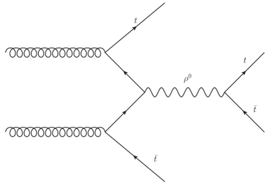
Figure 1: Typical Feynman diagram for process $gg\rightarrow t\bar{t}\rho\rightarrow t\bar{t}t\bar{t}$.

Both the production cross section and the decay width of these vector singlets are controlled by their coupling to top quarks. At typical LHC energies the top quark content of the proton can be neglected, rather we consider gluons in the initial state, splitting to high-$p_{T}$ top quark pairs. The leading tree-level production process occurs via $t\bar{t}$ scattering, singly-producing the vector resonance in association with a top-antitop pair. The resonance subsequently decays to another $t\bar{t}$ pair, resulting in a four-top final state (see Fig. 1).

Production via a top loop, analogous to gluon-gluon fusion in higgs production, is forbidden at leading order by the Landau-Yang theorem Landau:1948kw . The first non-zero contribution in the $t\bar{t}$ final state must thus occur at $\mathcal{O}(g_{s}^{6}g_{\rho}^{2})$, by emission of an additional hard jet; this process is formally higher-order in $g_{s}$ than the $t\bar{t}$ scattering process considered above, $\mathcal{O}(g_{s}^{4}g_{\rho}^{2})$, as well as suffering from larger Standard Model backgrounds.

There are also subleading effects that go in the opposite direction, enhancing the relative sensitivity of the gluon-fusion process. First, the cross section for the NLO top loop diagram will be enhanced by the valence quark component of the parton distribution function (PDF) in the initial state. The gluon-initiated component will also be enhanced since it is evaluated at a smaller centre-of-mass energy (no production of additional top quarks). . Finally, even though it suffers from a huge background from SM $t\bar{t}$, as mentioned above, its combinatorics are more tractable, allowing the resonance mass to be fully reconstructed in the semileptonic channel. A definitive answer as to which process drives the sensitivity for $\rho$ would require computation of the loop and box diagram contributions to $\rho$ production, in the limit of small top mass. We consider this to be beyond the scope of the current analysis, and reserve it for future work Liu:WIP . For the remainder of this paper, however, we will assume that the naive power counting argument holds, and focus on the four-top final state.

Selecting the parameters $M_{\rho}=1$ TeV, $g_{\rho}=1$ as a benchmark for illustrative purposes, the leading order cross section is 4.88 fb, with a width-to-mass ratio for the $\rho$, $\Gamma_{\rho}/M_{\rho}=3.6\%$. The branching fractions for decays to the different final states are set by those of the $W$ boson, the pure hadronic mode accounting for 31% of the events; the single-, di- and tri-lepton channels contributing 42%, 21% and 5% respectively, with the four-lepton channel contributing under 1%.

We plot the $p_{T}$ and $\eta$ distributions for truth-level top quarks, ordered by $p_{T}$, for $M_{\rho}=1$ TeV and $g_{\rho}$=1 in Fig. 2 below. One would nominally expect to see two hard, central tops coming from the resonance decay, with $p_{T}\sim M_{\rho}/2$ (= 500 GeV for our benchmark), and two softer tops with $p_{T}\sim m_{t}=$173 GeV. What we see instead is a rather more hierarchical spectrum after $p_{T}$-ordering, implying a mixing between top quarks from different origins. In fact, although the leading top comes from the $\rho$ decay almost 85% of the time, if we ask that the two hardest tops be daughters of the $\rho$, the probability falls to 50%. Note also that most of the top quarks are contained within the central region of the detector $|\eta|<2.5$, as expected. We also plot the average number of top quarks per event with $p_{T}>p_{T\text{min}}$ as a function of $p_{T\text{min}}$ for $M_{\rho}=1,\,2$ TeV in Fig. 2(c). We see that for resonance masses accessible at LHC14, we do not expect more than one top in each event to be highly boosted ($p_{T}>1$ TeV). The fully hadronic channel will thus contain a large number of well-separated jets, the combinatorics making it very hard to distinguish from QCD multijet background. At the other extreme, the four-lepton channel has too small a cross section. In this work we focus on the same-sign-dilepton channel, where we believe we will achieve the best significance due to small SM backgrounds.

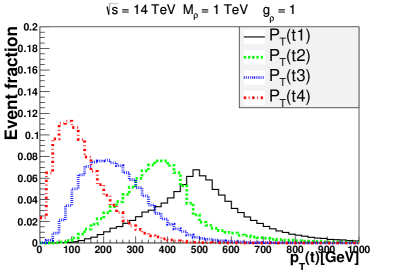
(a) $p_{T}$ distribution for truth-level top quarks in signal events with $M_{\rho}=$ 1 TeV and $g_{\rho}=1$, where tops are $p_{T}$-ordered.

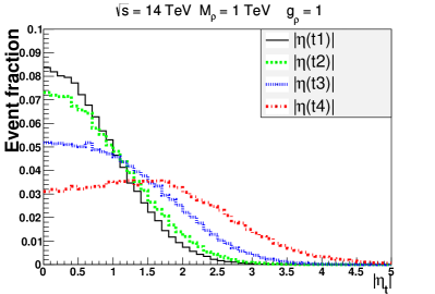
(b) $\eta$ distribution for truth-level top quarks in signal events with $M_{\rho}=$ 1 TeV and $g_{\rho}=1$, where tops are $p_{T}$-ordered.

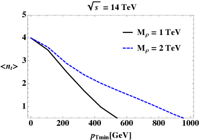
(c) The average number of truth-level tops per event with $p_{T}>p_{T\text{min}}$ as function of $p_{T\text{min}}$ for $M_{\rho}=$ 1 TeV (black solid ) and $M_{\rho}=$ 2 TeV (blue dashed).

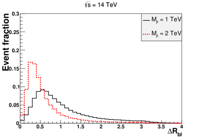
(d) Normalized $\Delta R_{b\ell}$ distribution for truth-level $b$ quark and lepton from daughter top quark, for $M_{\rho}=1$ TeV (black solid) and $M_{\rho}=2$ TeV (red dotted).

Figure 2: Truth-level distributions for top quarks and decay products in $pp\rightarrow t\bar{t}\rho\rightarrow t\bar{t}t\bar{t}$.

All results in this work were obtained by simulation using MadGraph5 Alwall:2011uj , interfaced to Pythia 6 Sjostrand:2006za for parton showering and hadronization as needed. For the signal, we have implemented the simplified model using FeynRules Feynrule in UFO format. We use the CTEQ6L1 parton distribution function (PDF), in the 4-flavour scheme , and the default event-by-event renormalization and factorization scales in MadEvent. FastJet Cacciari:2011ma was used to reconstruct narrow jets, using the pre-implemented anti-kt algorithm with $R=0.4$ Cacciari:2008gp . The signal was simulated at leading order; backgrounds were simulated using matrix element-parton shower merging and matching where necessary. This was done using MLM matching, with $p_{T}$-ordered showers in Pythia, in the ‘shower-kT’ scheme, where the matching scale (QCUT = XQCUT) varied between 30 and 40 GeV, depending on the process. The cross-section of electroweak-boson-plus-jet backgrounds were cross-checked using ALPGEN Mangano:2002ea , interfaced to Pythia 6 for showering and hadronization.

With increasing $M_{\rho}$, we expect the leptons coming from top decays will become increasingly collimated with the decay $b$-jet, failing the standard fixed-cone isolation criterion (with $\Delta R=0.3$) some non-negligible fraction of the time. This can be clearly seen in Fig. 2(d) above, where we plot the normalized parton-level $\Delta R_{b\ell}$ distribution for leptonically-decaying $\bar{t}$ in the signal, for two different resonance masses (1 and 2 TeV). In order to retain as much of the small signal cross section as possible, we use a modified lepton isolation criterion.

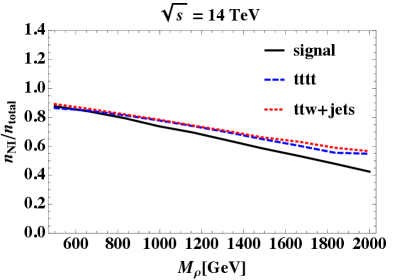
Figure 3: Ratio of normal- and mini-isolation efficiencies for leptons, for signal (black solid) and two dominant backgrounds: SM four-top (blue dashed) and $t\bar{t}W+$jets (red dotted), after all cuts.

This was proposed by Rehermann:2010vq as an efficient way to distinguish muons from top decays from those arising from heavy flavour decays, and was subsequently successfully tested in Monte Carlo studies of semileptonic top decays by ATLAS Chapleau:2010nn . The mini-isolation method involves applying an isolation criterion within a cone whose size varies inversely with lepton $p_{T}$ (this quantity can be seen as a measure of the boost of the parent) and requiring that the scalar sum of the hadronic $p_{T}$ inside such a cone centred on the lepton be less than 10% of the lepton $p_{T}$. Thus softer leptons are required to be more isolated than harder ones. In Fig. 3, we show the ratio of efficiencies for lepton selection with regular and mini-isolation for the signal and two dominant backgrounds. Although the efficiency ratio is similar for the signal and backgrounds, mini-isolation helps keep more events after cuts, thus improving the significance over the entire parameter space. This improvement is especially important at high resonance mass, where the production cross section is very small.

We define pre-selection cuts as follows:

$$p_{T,jcb}>30\,\text{GeV},\qquad|\eta_{j}|<4.5,\qquad|\eta_{cb}|<2.5$$ (2)

$$p_{T,\ell}>25\,\text{GeV},\qquad|\eta_{\ell}|<2.5,\qquad\sum\limits_{R_{\text{min}}}|p_{T,j}|\leq\;0.1\;p_{T,\ell}$$ (3)

where $p_{T}$ and $\eta$ denote the transverse momentum and pseudorapidity of the reconstructed jets and mini-isolated leptons as described above, and $R_{\text{min}}=\text{Min}(15/p_{T,\ell}\,,\,0.3)$. A reconstructed jet is identified as a b(c)-jet if its pseudorapidity satisfies $|\eta|<$ 2.5 and it is matched to a b(c)-parton at angular distance $\Delta R<0.2$. We then require exactly two same-sign leptons and at least 3 narrow jets. In order to reduce the backgrounds from di- and tri-boson plus jets, we stipulate at least 3 of the narrow jets be $b$-tagged. We assume constant $b$-tagging and mistagging efficiencies of 70% for $b$-jets, 20% for $c$-jets, and 1% for light jets, respectively. We discuss the validity of this assumption in Appendix B. The $b$-tagging requirement ensures the dominance of top-rich backgrounds, such as SM $t\bar{t}t\bar{t}$ and $t\bar{t}Wb\bar{b}$ production. There are also large contributions from backgrounds with mis-tagged jets such as $t\bar{t}W$ + jets, as well as subleading contributions from single-top in association with multiple vector bosons, where the vector bosons decay to charm jets (35% branching fraction for the $W$ boson). A list of all leading backgrounds with same-sign dileptons, including their cross sections after pre-selection and cut efficiencies, is shown in Table 1.

We plot in Fig. 4 the signal and background distributions for the number of $b$-jets after preselection, and the reconstructed $H_{T}$ distribution after requiring 3 $b$-tags, where $H_{T}$ is defined as the scalar sum of the $p_{T}$s of the leptons and all reconstructed jets in the event. This quantity can be used as a proxy for the scale of the hard scattering $\sim M_{\rho}+2m_{t}$, and as such, gives us some idea of the mass of the resonance, which would be tricky to obtain by event reconstruction due to combinatorics. To further suppress the backgrounds we put a hard cut on $H_{T}$, and require that this be larger than the mass of the resonance (=1 TeV for our benchmark model)

$$H_{T}=\sum\limits_{\text{all }j,\ell}\left|p_{T}\right|>M_{\rho}$$ (4)

We verify that we have sufficient statistics for all leading backgrounds, after all cuts have been imposed. We have not included K-factors in our results, since they are not contained in the literature for many of our background processes. We expect the K-factor for our signal to be similar to that for SM four-top production, which makes up a large component of the total background. We have also verified that changing the renormalization and factorization scale to the more conventional $m_{T}/3$, where $m_{T}$ is the transverse mass of the $t\bar{t}\rho$ system, increases the signal cross section by less than 20%.

Process	$\sigma_{\text{pre}}$ (ab)	Cut efficiencies		$\sigma$ (ab)
	SSDL + $n_{j}\geq$ 3	$n_{b}\geq$ 3	$H_{T}\geq 1$ TeV
Signal ($M_{\rho}=$ 1 TeV; $g_{\rho}=1$)	161	0.43	0.78	54.1
$t\bar{t}t\bar{t}$	224	0.39	0.37	31.9
$t\bar{t}W^{\pm}$+jets	$8.43\times 10^{3}$	0.026	0.16	34.2
$t\bar{t}Z$ + jets	$1.93\times 10^{3}$	0.024	0.14	6.71
$t\bar{t}(h\rightarrow W^{\pm}W^{*\mp}\rightarrow\ell\nu qq)$	$1.21\times 10^{3}$	0.043	0.11	5.77
$t\bar{t}W^{+}W^{-}$ + jets	295	0.04	0.29	3.44
$t\bar{t}W^{\pm}b\bar{b}$	21.6	0.31	0.22	1.50
$tbW^{+}W^{-}$	308	0.030	0.13	1.22
$tbW^{\pm}Z$	155	0.029	0.15	0.661
Total background				85.4

Table 1: Cross sections for the signal and leading backgrounds containing same-sign dileptons (SSDL) after preselection, cut efficiencies for $b$-tagging and $H_{T}$ cut, for $M_{\rho}=1$ TeV and $g_{\rho}=1$. The last column shows the final cross sections after all the selection cuts. Leading backgrounds are merged and matched, including up to two extra jets where relevant.

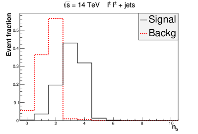
(a) Normalized distribution of number of b-jets, $n_{b}$ (defined in text) after preselection cuts.

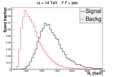
(b) Normalized $H_{T}$ distribution for all reconstructed jets and leptons after preselection and b-tagging.

Figure 4: Comparing distributions for signal $pp\rightarrow t\bar{t}\rho\rightarrow t\bar{t}t\bar{t}$ with SM backgrounds containing same-sign dileptons, after preselection (for a full list see Table 1).

Since the number of signal event is very small after all the cuts, we must also consider fake backgrounds, due to e.g. charge misidentification, or jets faking leptons. Contributing to the former will be $t\bar{t}+$j, and $Z+4b$; with semileptonic $t\bar{t}$ and $Wj+4b$ for the latter. We expect the $t\bar{t}$ background to be dominant in both instances, since it is produced at lower order in QCD. This expectation was confirmed in simulation, yielding a cross section after cuts of 2.62$\times 10^{3}$ ab in the dileptonic channel, and 6.17$\times 10^{4}$ ab in the semileptonic channel. We can make a crude estimate of the fake rate by applying a constant efficiency for each, based on the CMS and ATLAS TDRs CMS:TDR ; Aad:2009wy . Using 10^-3 for charge mis-ID and 10^-5 for jets-faking-leptons, for example, yields a contribution from fakes of less than 5% of the total background cross section, implying that these backgrounds are well under our control. In reality, however, the fake rates are strongly $p_{T}$-dependent, and a detailed experimental study would be required to confirm our estimate.

3 Results

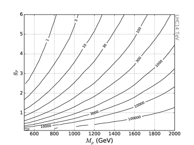
(a) Luminosity in fb^-1 required for discovery of spin-1 singlet resonance $\rho$ in SSDL channel of $4t$ final state, with 99.9999% confidence (corresponds to $5\sigma$ in large-statistics limit).

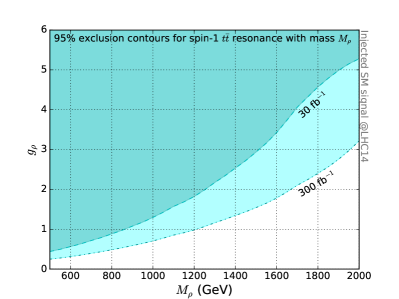
(b) Expected exclusion for singly-produced $\rho$ in SSDL channel of $4t$ final state, at 95% confidence with SM signal injection and luminosity of 30 (300) fb^-1.

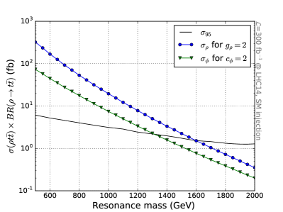
(c) 95% expected upper limit on $\sigma\times BR$ for $t\bar{t}$ resonance produced in association with a top-antitop pair with luminosity of 300 fb^-1 .

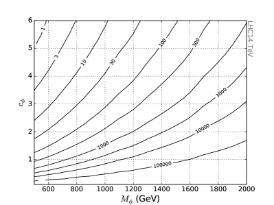
(d) Luminosity in fb^-1 required for discovery of singlet scalar $\phi$ in SSDL channel of $4t$ final state, with 99.9999% confidence (corresponds to $5\sigma$ in large-statistics limit).

Figure 5: Discovery/exclusion potential for gauge singlet $t\bar{t}$ resonance at LHC14 in $4t$ final state.

Our final results are shown in Fig. 5, with the statistical procedure used to obtain them summarized in Appendix D. In Fig. 5(a), we plot isocontours of the integrated luminosity required for discovery of a gauge singlet spin-1 $t\bar{t}$ resonance at LHC14. We naively rescale the signal cross section computed for a coupling of unity with $g_{\rho}$, in the narrow width approximation, ignoring interference effects with SM 4-top production. We justify this simplification in Appendix C.

We see that at moderate (large) coupling, $g_{\rho}=3\,(6)$, 300 fb^-1 of integrated luminosity at LHC14 will allow us to discover a spin-1 singlet resonance up to $\sim$1.5 (1.9) TeV. Discovery of a resonance with smaller coupling, say $g_{\rho}$=2, seems unlikely for masses larger than $\sim$ 1.3 TeV before the high-luminosity upgrade of the LHC, although exclusion of this region of parameter space should be possible with 95% probability by the end of LHC Run 3 (see Fig. 5(b)).

Our results can also be used to compute the discovery reach/exclusion potential in the $4t$ channel for any $t\bar{t}$ resonance that is singly produced in association with a top-antitop pair, where the kinematics (and hence the cut efficiencies) are likely to be similar to those of the vector resonance. For ease of recasting, we present our results as a 95% exclusion limit on $\sigma\times BR$ for this channel as a function of the resonance mass with an integrated luminosity of 300 fb^-1 in Fig. 5(c).

In particular we can trivially estimate the discovery luminosity required for a spin-0 resonance $\phi$, with a chiral-symmetry breaking coupling to top quarks of $c_{\phi}\,\phi\,\bar{t}_{L}\,\,t_{R}+\text{h.c.}$ Such a scalar could be found in a (fine-tuned) corner of the MSSM parameter space, for example, as the heavy higgs in the pseudoscalar decoupling limit, and for $\tan{\beta}\lesssim 3$. Alternatively it could be the heavy pseudoscalar resonance in Superconformal Technicolor theories Azatov:2011ps . The size of the coupling $c_{\phi}$ will depend on the representation of $\phi$ under the SM weak gauge group, $SU(2)_{L}$. If it is a doublet, then $c_{\phi}$ can be $\mathcal{O}(1)$. If it is an electroweak singlet, however, then the above coupling is strongly suppressed, since it originates in a dimension-5 operator involving the higgs field, with a coefficient $c_{\phi}=g_{\phi}m_{t}/\Lambda$, for a cutoff $\Lambda$ that is parametrically larger than the $\phi$ mass. The size of $g_{\phi}$ will depend on the origin of the interaction, for a weakly-coupled theory it must be of $\mathcal{O}(y_{t})$, but it can be larger if it originates from a strongly-coupled sector.

Since the scalar couples to left-handed (LH) as well as RH top quarks, we might expect the efficiency for lepton selection to change, since leptons originating from decays of LH tops have smaller $p_{T}$, due to preferential emission antiparallel to the parent top quark’s boost. However we expect this to be a small effect, and hence apply the $\rho$ efficiencies naively. We show the luminosity isocontours required for discovery of a scalar resonance in Fig. 5(d). As expected, the results for a scalar resonance are not quite as encouraging as those for the vector resonance, particularly if the scalar is a gauge-singlet elementary field, in which case $c_{\phi}$ is constrained to be rather small. Instead, we expect the sensitivity for the scalar resonance to be driven by the $t\bar{t}$ final state, since the gluon-fusion production is unsuppressed, and rather large.

In principle it should be possible to compare the sensitivity of our analysis to that of other searches for $t\bar{t}$ resonances. One example is the 8 TeV ATLAS resonance search in the lepton-plus-jets channel of the $4t$ final state Aad:2015kqa . Their results are presented in the form of exclusion limits on $\sigma\times BR$, but here the benchmark resonances used to obtain these results are pair-produced, resulting in a much larger $H_{T}$ in the final state than in the case of single production, for a resonance with equal mass. This would give rise to large differences in the efficiencies for their $H_{T}$ cuts, and we cannot simply recast their limits in the context of our simplified model.

ATLAS also present their results as limits on the coupling of a four-top contact interaction of the following form:

$$\frac{C_{4t}}{\Lambda^{2}}\left(\bar{t}_{R}\gamma^{\mu}t_{R}\right)\left(\bar{t}_{R}\gamma_{\mu}t_{R}\right)$$ (5)

which might also be useful for the purposes of comparison. Using a likelihood fit to the $H_{T}$ spectrum after cuts to LHC data at 8 TeV centre-of-mass energy, they obtain a 95% CL upper limit on the coefficient of the 4$t$ contact interaction $|C_{4t}|/\Lambda^{2}<6.6$ TeV^-2. By integrating out the $t\bar{t}$ resonance, we can naively interpret this as a limit on the relevant combination of our simplified model parameters, yielding $M_{\rho}/g_{\rho}>275$ GeV. However, care must be taken to ensure that this limit is consistent with the effective theory being used within its regime of validity in the analysis. In this particular instance the limit is obtained by a comparison of their measured $H_{T}$ distribution to that expected from signals and backgrounds, over the entire range of $H_{T}$ measured ($\sim$ 2 TeV). In the absence of any information to the contrary, we have to assume that the entire range of $H_{T}$ was equally instrumental in deriving the limit, and since $H_{T}$ can be thought of as a lower bound for the centre-of-mass energy, their limit can only be applied for $M_{\rho}>2$ TeV. Hence their limit cannot be applied for $g_{\rho}\lesssim 7$!

When set in the broader context of a realistic scenario, there will also be additional constraints on singlet bosons due to their subleading interactions. We will explore some of these in the context of the $SO(5)/SO(4)$ composite higgs in Section 4 below.

4 Interpretation in Composite Higgs framework

The encouraging results obtained in the large-coupling region of our simplified models beg for an interpretation within the Composite Higgs (CH) framework, in which the Higgs arises as a pseudo-goldstone boson of some larger global symmetry (see Contino:2010rs ; Panico:2015jxa for a comprehensive review, and references therein). The presence of spin-1 resonances is a robust prediction in this framework, as they can be excited from the vaccum by the conserved currents in the strong sector. In typical CH models, however, it is the composite fermion resonances that are usually assumed to be among the lightest new states in the theory, since these are expected to cut off the large top-quark loop contribution to the quadratic divergence of the higgs mass. Furthermore, there are usually strong constraints on the mass of vector resonances that are electroweak- or colour-charged, from precision electroweak measurements, and flavour-changing neutral currents, respectively. These stringent limits do not apply to singlet resonances however, hence there is no theoretical bias against a composite vector resonance being the lightest new particle in the theory, provided it is a gauge singlet.

A gauge-singlet spin-1 resonance is, in fact, present in many simple incarnations of this scenario, excited by the conserved current of a global $U(1)_{X}$ symmetry group. Such a group is required in order to correctly reproduce the hypercharge of the RH top quark, in (more minimal) scenarios where the $t_{R}$ is a composite singlet of the strong-sector global symmetries. This resonance, which we denote as $\rho_{X}$, only interacts with elementary fermions through small mixing terms, suppressed by powers of the ratio $g^{\prime}/g_{\rho_{X}}$, where $g^{\prime}$ is the coupling of the SM hypercharge gauge boson (which mediates the coupling of $\rho_{X}$ with the rest of the elementary sector via a linear mixing), and $g_{\rho_{X}}$ is a large coupling typical of the composite sector. Among the SM fermions, the right-handed top alone is not constrained to be a purely elementary field; in the case that it is a fully composite singlet under the global symmetries, it could have a large coupling to $\rho_{X}$, as in the CH model with a minimal $SO(5)/SO(4)$ coset structure:

$$\mathcal{L}_{\rho_{X}}=-\frac{1}{4}\rho_{\mu\nu}^{X}\rho^{X\mu\nu}+\frac{m_{\rho_{X}}^{2}}{2g_{\rho_{X}}^{2}}(g_{\rho_{X}}\rho^{X}_{\mu}-g_{el}^{\prime}B_{\mu})^{2}\,+c\,\bar{t}_{R}\gamma^{\mu}(g_{\rho_{X}}\rho^{X}_{\mu}-g_{el}^{\prime}B_{\mu})t_{R}+\cdots$$ (6)

Here $c$ is an $\mathcal{O}(1)$ parameter which we set equal to 1 for simplicity, and we are omitting additional higher derivative interactions that stem from the CCWZ construction. The full lagrangian and interactions can be found in  Greco:2014aza , with important intermediate results summarized in Appendix E for convenience.

As mentioned above, through linear mixing with the SM hypercharge gauge boson, $\rho_{X}$ will also acquire (mixing-suppressed) couplings to other SM states, such as $W$ bosons and elementary quarks. These give rise to additional production mechanisms for $\rho_{X}$, via vector-boson fusion (VBF), or a Drell-Yan-like process $q\bar{q}\rightarrow\rho_{X}\rightarrow t\bar{t}$, as well as additional decay modes. Drell-Yan production is suppressed with respect to production via $t\bar{t}$ fusion considered above, by a factor of $g^{\prime 4}/(g_{\rho_{X}}g_{s})^{4}$ ; VBF is further suppressed by the $W$ PDF inside the proton, and is effectively negligible Greco:2014aza ; Pappadopulo:2014qza . In the large mass region, however, the top fusion channel falls much faster than the Drell-Yan contribution, due to the steep drop of the gluon PDFs at large $x$. We show the competing effect of $\rho_{X}$ production in the two leading channels, as well as its decay branching fractions for fixed mass (branching fractions are almost independent of mass in the large $M_{\rho}$ limit) in Fig. 6.

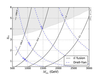
(a) Cross section contours (fb) for on-shell production of the $\rho_{X}$ The black solid (blue dashed) line corresponds to the production via $t\bar{t}$ fusion (Drell-Yan type production). The $t\bar{t}$ fusion cross section dominates in the shaded region.

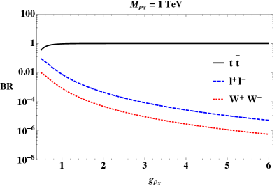
(b) $\rho_{X}$ branching fraction as a function of coupling $g_{\rho_{X}}$ (mass-independent for large $M_{\rho_{X}}$).

Figure 6: Production cross section [fb] and decay branching fraction for spin-1 singlet boson $\rho_{X}$, with coupling $g_{\rho_{X}}$ to RH tops, and a mixing-suppressed coupling $g^{\prime}/g_{\rho_{X}}$ to elementary fermions.

In the small-coupling region, it may be more effective to search for the $\rho_{X}$ boson in one of its alternative decay modes, via Drell-Yan type production. Various searches in relevant channels have been carried out by the ATLAS and CMS experiments, with results presented in terms of limits on $\sigma\times BR$ for each channel. The search with the largest sensitivity over the entire range of $\rho_{X}$ masses considered in this work are the ATLAS and CMS high-mass dilepton resonance searches Aad:2014cka ; Khachatryan:2014fba . Since $\sigma\times BR$ in this channel scales like $(g^{\prime 4}/g_{\rho_{X}}^{2})\times(g^{\prime}/g_{\rho_{X}})^{4}$, however, the limit becomes quickly irrelevant above $g_{\rho_{X}}\sim 1.2$, where the ATLAS $t\bar{t}$ Aad:2015fna search takes over in sensitivity, the branching ratio to $t\bar{t}$ exceeding 90% above $g_{\rho_{X}}=1$ (see Fig. 6(b)). Other searches, e.g. in the $WW$Aad:2015ufa ; Aad:2015owa ; Khachatryan:2014gha ; Khachatryan:2014hpa , $ZH$ Aad:2015yza ; Khachatryan:2015bma ; Khachatryan:2015ywa and $\tau\tau$ channels Aad:2015osa , as well as searches in dijets Khachatryan:2015sja , have negligible sensitivity and are not considered here. Fig. 7 below we show the exclusion limits on the $\rho_{X}$ parameter space recast from the two most sensitive analyses, the ATLAS $t\bar{t}$ Aad:2015fna and CMS dilepton searches Khachatryan:2014fba . We see that the strategy advocated in this paper is exactly complementary to existing searches in other channels, giving an enhanced sensitivity at large $g_{\rho_{X}}$, which is not accessible by other means. Note that only the Drell-Yan-type production cross section was used to set the limit in the $t\bar{t}$ channel. In principle there will also be a contribution due to gluon-gluon fusion

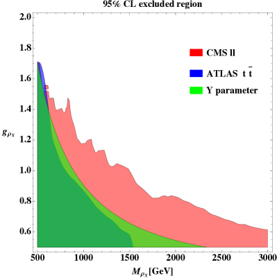
Figure 7: Current limits on the $\rho_{X}$ parameter space in CH models from most sensitive 8 TeV analyses: CMS dilepton search Khachatryan:2014fba and ATLAS $t\bar{t}$ Aad:2015fna . We also include the constraint from the electroweak $Y$ parameter (details in text).

at next-to-leading order, but we expect this to be negligible in the range of $g_{\rho_{X}}$ constrained here. Care must be taken in translating these limits on $g_{\rho_{X}}$ to limits on the simplified model parameter $g_{\rho}$, which are related as detailed in Appendix E. Their difference is negligible in the limit of large $g_{\rho_{X}}$, but could be significant, and model dependent, for small values.

There are additional constraints on the mass and coupling of $\rho_{X}$, coming from precision electroweak observables. The $Y$-parameter, the 2nd derivative of the hypercharge form factor Barbieri:2004qk , is the leading constraint here, since there is no contribution to the $S$ parameter from a singlet. To compute the contribution to this low-energy observable from $\rho_{X}$ we simply integrate it out by setting it equal to its equation of motion, giving at leading order in the derivative expansion, the following terms in the effective lagrangian

$$\mathcal{L}_{\text{eff}}\supset-\frac{1}{2}\frac{g_{\rho_{X}}^{2}}{m_{\rho_{X}}^{2}}\bar{t}_{R}\gamma^{\mu}t_{R}\bar{t}_{R}\gamma_{\mu}t_{R}-\frac{1}{2}\frac{g^{\prime 2}}{g_{\rho_{X}}^{2}m_{\rho_{X}}^{2}}\partial^{\mu}B_{\mu\nu}\partial_{\alpha}B^{\alpha\nu}$$ (7)

The second term yields an expression for $Y$ at tree-level, which can be constrained using the global fit in Barbieri:2004qk :

$$|Y|=\frac{g^{\prime 2}m_{W}^{2}}{g_{\rho_{X}}^{2}m_{\rho_{X}}^{2}}<1.2\times 10^{-3}\Rightarrow g_{\rho_{X}}m_{\rho_{X}}\geq 836\;\text{GeV}$$ (8)

This is a rather weak limit; $Y$ is usually suppressed with respect to the $S$-parameter by a factor of $g^{\prime 2}/g_{\rho_{X}}^{2}$. We see in Fig. 7(b) that this constraint is comparable to that from the ATLAS $t\bar{t}$ search, which is, itself, not very constraining for large values of $g_{\rho_{X}}$. It is easy to see in this plot the complementarity between the sensitivity of current search strategies, and the strategy we advocate in this paper. It is clear that $t\bar{t}$ fusion drives the sensitivity at larger couplings.

5 Conclusion

In this paper, we studied the reach for a top-antitop vector resonance in the same-sign dilepton channel of the 4-top final state at LHC14. For a vector resonance that couples dominantly to top quarks, this $t\bar{t}$ fusion channel is the leading tree-level production mode; single production via a top loop being forbidden by Yang’s theorem. Our analysis made use of the large $b$-jet multiplicity of the signal, as compared with the background, as well as the relative paucity of Standard Model backgrounds with same-sign dileptons. Due to the large combinatorics of the 4-top final state, we did not attempt a full reconstruction of the event, placing instead, a hard $H_{T}$ cut on the reconstructed objects in the final state in order to select events with higher centre-of-mass energies. We found that the irreducible SM 4-top background, which was omitted in a similar search, was a dominant component of the background after cuts.

We presented our results in the form of isocontours of luminosity required for discovery, in the parameter space (mass, coupling) of the resonance, as well as a 95% exclusion limit on the cross-section $\times$ branching ratio in this final state (see Figs. 5). We found a discovery reach (95% exclusion) for vector resonances with 300 fb^-1 integrated luminosity, of mass up to 1.2 (1.6) TeV for a coupling to right-handed tops, $g_{\rho}=$2. We also placed limits on a scalar $t\bar{t}$ resonance, although we expect the sensitivity in this case will be larger in the $t\bar{t}$ final state.

We interpreted our results within Composite Higgs scenarios, many simple implementations of which contain a singlet vector resonance $\rho_{X}$, excited from the vacuum by the conserved current of a $U(1)_{X}$ global symmetry. These vector singlets can have a large coupling to RH top quarks in the case where the latter are composite singlets of the strong sector. However they only interact with other SM particles via a linear mixing with $B^{\mu}$, the hypercharge boson, resulting in couplings that scale parametrically as $g^{\prime}/g_{\rho_{X}}$. Hence direct searches for these resonances decaying to pairs of Higgs/gauge bosons, leptons, or light jets, have maximum sensitivity for small $g_{\rho_{X}}$. The most efficient way to access the region of large $g_{\rho_{X}}$ is likely through the four-top final state. Unfortunately existing resonance searches in the four-top channel are not directly applicable to this class of models, since their results are expressed either in terms of benchmarks with pair-produced resonances, or limits on the coefficient of a four-top contact interaction. For a light resonance that is singly-produced via $t\bar{t}$ fusion, neither one applies. Its cut efficiencies, particularly for hard $H_{T}$ cuts, are likely to be considerably smaller than the corresponding ones for a pair-produced resonance of the same mass. Moreover, the analysis appears to obtain much of its sensitivity from events with a large centre-of-mass energy (up to $H_{T}=2$ TeV), and hence cannot be used to place limits on a four-top contact interaction obtained by integrating out a resonance with mass smaller than this scale. For these reasons, we strongly urge the relevant experimental groups to include in their benchmarks an example of a resonance that is singly-produced, in association with tops, in order to improve their coverage of the available theory space in this rather well-motivated scenario.

Appendix A Cross section tables

In this appendix, we present the cross sections under different mass hypotheses for the spin-1 (Table 2) and scalar (Table 3) resonances, for production through $t\bar{t}$ fusion with unit coupling $g_{\rho}=c_{\phi}=1$. These cross sections were used in our determination of the 95% upper limit for the cross section. The cross sections were calculated using the MadGraph5 Alwall:2011uj , using the default event-by-event factorization and renormalization scales. We also show the final cross sections for the signal and the total backgrounds after all the cuts for the spin-1 resonance $\rho$. In addition, we present in Table 2 the naive significance, $S/\sqrt{B}$, for the integrated luminosity of 300 fb^-1.

$M_{\rho}$ [GeV]	500	600	700	800	900	1000	1100	1200
$\sigma_{\rho}$[fb]	80.6	42.0	23.1	13.3	7.93	4.88	3.05	1.95
$\sigma_{S}$[ab]	854	470	262	151	89.4	54.1	32.3	21.0
$\sigma_{B}$[ab]	309	250	197	151	114	85.4	64.0	47.1
$S/\sqrt{B}$	27	16	10	6.8	4.6	3.2	2.2	1.7
$M_{\rho}$ [GeV]	1300	1400	1500	1600	1700	1800	1900	2000
$\sigma_{\rho}$[fb]	1.26	0.834	0.562	0.379	0.261	0.181	0.126	0.0883
$\sigma_{S}$[ab]	12.8	8.22	5.40	3.53	2.22	1.52	1.02	0.668
$\sigma_{B}$[ab]	34.0	24.7	18.0	13.4	10.1	7.82	5.98	4.61
$S/\sqrt{B}$	1.2	0.91	0.70	0.53	0.38	0.30	0.23	0.17

Table 2: Production cross section, $\sigma_{\rho}$ for spin-1 resonance of mass $M_{\rho}$ for fixed coupling to the right-handed top quark $g_{\rho}$ = 1. Also shown is cross section after cuts ($\sigma_{S}$), background cross section ($\sigma_{B}$), and naive significance, $S/\sqrt{B}$, for integrated luminosity of 300 fb^-1.

$M_{\phi}$ [GeV]	500	600	700	800	900	1000	1100	1200
$\sigma_{\phi}$ [fb]	18.3	11.1	6.9	4.4	2.8	1.9	1.2	0.84
$M_{\phi}$ [GeV]	1300	1400	1500	1600	1700	1800	1900	2000
$\sigma_{\phi}$ [fb]	0.57	0.40	0.27	0.19	0.14	0.097	0.069	0.050

Table 3: Production cross section for spin-0 resonance of mass $M_{\phi}$, and coupling to tops $c_{\phi}$=1.

Appendix B B-tagging efficiency

In this appendix, we want to make some comments on the constant b-tagging(mistagging) efficiency used in our analysis. As is well known, the b-tagging (c-mistagging) efficiency will decrease when the $p_{T}$ becomes too large ($p_{T}\gtrsim 450$ GeV). Although the mistagging rate for the light jets will increase by a factor of 2, it is not relevant in our case, because the backgrounds originating from the light jets are two small. Our signature is mainly coming from the $3b,4b$ configuration for the SM four top background and $2b1c$ for the $t\bar{t}W+jets$. So both the signal and the background will be reduced for the large transverse momentum. To emphasize how large its impact, we plot in Fig. 8 the average number of b-jets, c-jets per-event with $p_{T}>450\text{GeV},|\eta|<2.5$ after the $H_{T}$ cut for the signal and the main background as a function of the of the resonance. From the figure, we can infer that for the signal, the effect of varying b-tagging efficiency is quite mild and it reduces the number of event by $\sim 25\%$ for the signal with $M_{\rho}=2$ TeV if we assume that the b-tagging efficiency go down from $70\%$ to $50\%$ when $p_{T}\gtrsim 450$ GeV. When the reduction of the backgrounds are also considered, the effects on the significance $S/\sqrt{B}$ are further going down to $\sim 20\%$. So we conclude that the constant b-tagging efficiency is a good approximation in our analysis.

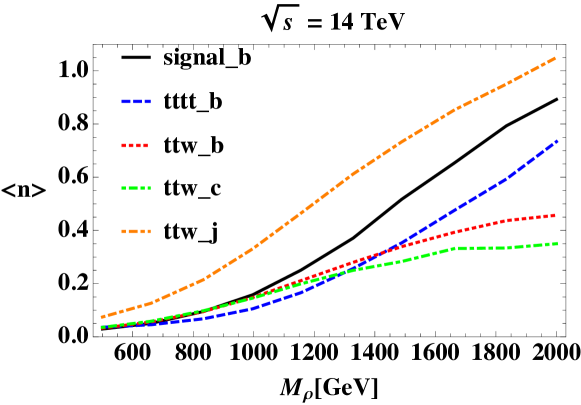
Figure 8: The average number of b-jets, c-jets, light-jets with $p_{T}>450$ GeV after the $H_{T}$ cut for the signal and the background as a function of the mass $M_{\rho}$. We have set the minimal value of $H_{T}$ to $M_{\rho}$ for each mass hypothesis. The black solid line and blue dashed line correspond to the number of b-jets for the singal and the SM four top background separately. The other three lines mean the number of b-jets (in read dotted), c-jets(in green dotted-dashed ), light-jets(in orange dotted-dashed) for $t\bar{t}W+jets$.

Appendix C The finite width effect

As studied in Ref. Pappadopulo:2014qza , two kinds of important effects due to the finite decay width are present in the searches of resonances. One is the distortion of the signal shape, as a consequence of the sharp falling of the PDF at large x, the other is the interference with SM 4 top background. Since $\rho$ is strongly interacting with right-handed top, it is usually much broader than the other resonances. Neglecting the top mass, the decay-width-mass ratio is roughly $\Gamma_{\rho}/M_{\rho}\sim(1/8\pi)g_{\rho}^{2}\sim 0.04g_{\rho}^{2}$, which means that for $g_{\rho}\gtrsim 5$, the ratio is already larger than 1. In this case, it is questionable whether we can treat it as a particle or not. Possibly contact interactions should be studied. In this section, we will study the effect of decay width on the optimal cuts we imposed by adopting $g_{\rho}=1,2,3,4,5$ for $M_{\rho}=1$ TeV and 2 TeV. Our result is evidently not conclusive, the dedicated analysis should be performed by the experimental collaborations. Let’s start from the effect due to the PDF. The number of signal after all the selection cuts can be parametrized as:

$$\begin{split}n_{s}(M_{\rho},g_{\rho})&=\sigma_{0}(M_{\rho},g_{\rho},\Gamma(M_{\rho},g_{\rho}))\times\epsilon(M_{\rho},\Gamma(M_{\rho},g_{\rho}))\times L\end{split}$$ (9)

where $\sigma_{0}$ is the cross section for the process $pp\rightarrow\rho t\bar{t}\rightarrow t\bar{t}t\bar{t}$ before any cuts and $L$ is the integrated luminosity. In general, the efficiency $\epsilon$ also depends on the finite decay widths. Things will be simplified when the resonance is narrow and using NWA, the coupling $g_{\rho}$ can be totally factorized as (for detail, see Ref. Pappadopulo:2014qza )

$$\begin{split}n_{s}(M_{\rho},g_{\rho})&=g_{\rho}^{2}\times\sigma_{0}(M_{\rho})\times\epsilon(M_{\rho})\times L\end{split}$$ (10)

where we neglect the finite decay width effects on the kinematics of the decay products. This is the formula we used when drawing the Fig. 5. As the decay width ratio $\Gamma_{\rho}/M_{\rho}$ becomes large, which is the case for large $g_{\rho}$, this procedure becomes less precise. In the following, we will quantify the finite width effects by showing the two ratios:

$$\begin{split}R_{1}&=\sigma_{0}(M_{\rho},g_{\rho},\Gamma(M_{\rho},g_{\rho}))/g_{\rho}^{2}\sigma_{0}(M_{\rho},1,\Gamma(M_{\rho},1)),\\ R_{2}&=\epsilon(M_{\rho},\Gamma(M_{\rho},g_{\rho}))/\epsilon(M_{\rho},\Gamma(M_{\rho},1))\end{split}$$ (11)

for the cases of $M_{\rho}=1,2$ TeV, $g_{\rho}=2,3,4,5$. Scanning over the two parameter space is beyond the scope of the paper.

From Table 4, we can see that the total cross sections get a sizable contribution from the kinematical region, where the invariant mass of the two tops from the $\rho$ decay departs from the peak region around $M_{\rho}$. The relative difference from naive scaling for the inclusive cross section is increasing from $16\%$ to $74\%$ as $g_{\rho}$ varying from 2 to 5 for $M_{\rho}=1$ TeV. For $M_{\rho}=2$ TeV, the situation gets worser, because it is probing the large $x$ of the gluon PDF, which drops faster. The point has already been discussed in Ref. Pappadopulo:2014qza . For the ratio $R_{2}$, the efficiency is reduced for larger value of $g_{\rho}$ as expected. For comparison, we also show the numbers of $R_{1}\times R_{2}$, which really matter in reality. Although the inclusive cross section and the efficiency differ a lot from naive scaling, the product of them seems well under control for $M_{\rho}=1(2)$ TeV, which is within $15(25)\%$ even for $g_{\rho}=5$. Nevertheless, our naive scaling is at least a conservative estimate for the large $g_{\rho}$.

Couplings	$g_{\rho}=2$	$g_{\rho}$ = 3	$g_{\rho}$ = 4	$g_{\rho}$ = 5
$R_{1}(M_{\rho}=$ 1 TeV )	1.16	1.39	1.61	1.74
$R_{2}(M_{\rho}=$ 1 TeV )	0.835	0.743	0.665	0.658
$R_{1}\times R_{2}(M_{\rho}=$ 1 TeV )	0.970	1.03	1.07	1.14
$R_{1}(M_{\rho}=$ 2 TeV )	2.02	3.41	4.57	5.08
$R_{2}(M_{\rho}=$ 2 TeV )	0.511	0.313	0.261	0.240
$R_{1}\times R_{2}(M_{\rho}=$ 2 TeV )	1.03	1.07	1.19	1.22

Table 4: Relative efficiencies after all the selection cuts under the different couplings of the $\rho$ resonance.

As regards with the inteference with SM four top background, we have calculated the total cross section including the interference terms and compare them with direct sum of the cross sections. It turn out that the interference effects are well under control in our case and rarely exceed 10%. This can be due to the fact that the relevance of the interference term is dertermined by the two competing effects: the decay width and the ratio between the signal and the four top background. The larger the decay width and the smaller the signal to background ratio, the more important for the interference contribution. But in our case, both of them are fixed by the same parameter $g_{\rho}$ and have the same scaling $\sim g_{\rho}^{2}$, which cancelled with each other and resulted in the quite mild behaviour for the interference term.

Appendix D Statistical tools

To obtain our final results, following Contino:2012xk we define a Bayesian posterior probability $p_{\mathcal{L}}(\sigma|N_{\text{obs}})$ of a total event cross section, $\sigma$, given an observed number of events, $N_{\text{obs}}$, at an integrated luminosity, $\mathcal{L}$, as the product of a Poissonian likelihood function $L(N_{\text{obs}}|\sigma\mathcal{L})$ and a prior $\pi(\sigma)$:

$$p_{\mathcal{L}}(\sigma|N_{\text{obs}})\propto L(N_{\text{obs}}|\,\sigma\mathcal{L})\;\pi(\sigma)$$ (12)

where

$$L(N|\,\sigma\mathcal{L})=\frac{\exp^{-\sigma\mathcal{L}}\left(\sigma\mathcal{L}\right)^{N_{\text{obs}}}}{N_{\text{obs}}!}$$ (13)

is the poissonian probability of observing $N_{\text{obs}}$ events, with a given process cross-section and integrated luminosity.

In order to obtain the discovery contours of Figs. 5(a) and (d), we take a prior that is flat for all $r>0$, and vanishing otherwise, and normalize the probability such that

$$\int_{0}^{\infty}d\sigma\;p_{\mathcal{L}}(\sigma|N)=1$$ (14)

We then compute, at each point in the ($m_{\rho},g_{\rho}$) parameter space, corresponding to a given signal and background cross-section ($\sigma_{S}$ and $\sigma_{B}$), the smallest luminosity at which there are more than 5 observed events $(\sigma_{S}+\sigma_{B})\mathcal{L}\geq 5$, and the following inequality is satisfied:

$$\int_{0}^{\sigma_{B}}d\sigma^{\prime}\,p_{\mathcal{L}}\!\left(\sigma^{\prime}\big{|}(\sigma_{S}+\sigma_{B})\mathcal{L}\right)\leq 5.7\times 10^{-7}.$$ (15)

This corresponds to the possibility of a cross section smaller than or equal to that of the background being consistent with a measured total number $(\sigma_{S}+\sigma_{B})\mathcal{L}$ events occuring less than $5\times 10^{-5}\%$ of the time (=5$\sigma$ in the large statistics limit).

To obtain the parameter measurement plot in Fig. 5(b) we normalize the posterior probability independently at each resonance mass, with a prior distribution that is flat over the range of couplings $g_{\rho}$ in $(0,4\pi)$ as $\int dg_{\rho}\;p_{\mathcal{L}}\!\left(\sigma(M_{\rho},g_{\rho})\big{|}N_{\text{obs}}\right)=1$ and compute the value of the coupling at which the posterior probability with injection of the SM contained within the region is 5%. Note that this procedure is sensitive to the choice of prior, if the boundary is placed in a region where the probability is changing rapidly.

To obtain the 95% upper limit on the cross section, we follow the procedure above, except we normalize the posterior probability with a flat prior over the range $\sigma$ in $(0,\infty)$. Note, however, that the appropriate lower limit will depend on the model in question; in the case of the $SO(5)/SO(4)$ Composite Higgs model, for example, $g_{\rho_{X}}$ must be larger than the SM hypercharge coupling $g^{\prime}$. This is a consequence of the same prior-dependence noted above. The result is much less sensitive to the choice of upper limit, since the posterior probability for much of the range of large $\sigma$ is negligible.

Appendix E Vector singlet in $SO(5)/SO(4)$ Composite Higgs model

We briefly review the properties of the $\rho_{X}$ composite vector singlet in the $SO(5)/SO(4)$ CH model below.For a detailed exposition and analysis, see Greco:2014aza ; Contino:2011np . In the limit $M_{*}\gg M_{\rho_{X}}$, where $M_{*}$ is the mass scale of all the other bounds states of the strong sector, we can integrate out all other heavy resonances, giving, at leading order in the derivative expansion, the following effective lagrangian:

$$\begin{split}\mathcal{L}=&\quad-\frac{1}{4}W_{\mu\nu}^{a}W^{a\,\mu\nu}-\frac{1}{4}B_{\mu\nu}B^{\mu\nu}+\bar{\psi}\gamma^{\mu}\!\left(i\partial_{\mu}+g_{el}\frac{\sigma^{a}}{2}W_{\mu}^{a}P_{L}+Yg_{el}^{\prime}B_{\mu}\right)\!\psi+\frac{f^{2}}{4}(d_{\mu}^{\hat{a}})^{2}\\ &-\frac{1}{4}\rho_{X\mu\nu}\rho^{\mu\nu}_{X}+\frac{M_{\rho_{X}}^{2}}{2g_{\rho_{X}}^{2}}(g_{\rho_{X}}\rho_{X\mu}-g_{el}^{\prime}B_{\mu})^{2}\,+c\,\bar{t}_{R}\gamma^{\mu}(g_{\rho_{X}}\rho_{\mu}-g_{el}^{\prime}B_{\mu})t_{R},\\ \end{split}$$ (16)

where $g_{el}$ are the proto-electroweak gauge couplings, $c$ is an $\mathcal{O}(1)$ parameter and $\psi$ stands for all the SM fermions.. Here we assume that the RH top quark is a chiral singlet bound state of the strong sector, which allows it to couple directly to $\rho_{X}$ as shown above. $d_{\mu}^{\hat{a}}$ is defined via the CCWZ construction as a function of the $SO(5)/SO(4)$ Nambu-Goldstone matrix $U$:

$$-iU^{\dagger}D_{\mu}U=d_{\mu}+E_{\mu}\,,$$ (17)

where $U=\text{exp}(i\sqrt{2}\pi^{\hat{a}}T^{\hat{a}}/f)$. Under a general $SO(5)$ rotation $g\,\in\,SO(5)$, this is subject to the unbroken $SO(4)$ transformation as follows:

$$U\rightarrow g\,U\,h(x)^{\dagger},\qquad d_{\mu}\rightarrow h(x)\,d_{\mu}\,h(x)^{\dagger},\qquad E_{\mu}\rightarrow h(x)\,E_{\mu}\,h(x)^{\dagger}-ih(x)\,\partial_{\mu}h(x)^{\dagger}$$ (18)

where $h(x)\in SO(4)$ is a complicated function of $(\pi(x),g)$. Going to unitary gauge after EWSB:

$$d_{\mu}^{\hat{a}} =-\frac{\sin(\theta+h/f)}{\sqrt{2}}\delta^{\hat{a}\hat{i}}\left(g_{el}W_{\mu}^{\hat{i}}-g^{\prime}_{el}\delta^{\hat{i}3}B_{\mu}\right)+\sqrt{2}\frac{\partial_{\mu}h}{f}\delta^{\hat{a}4},$$

$$E_{\mu}^{aL} =-\left(\frac{1+\cos(\theta+h/f)}{2}\right)g_{el}W_{\mu}^{a}-\delta^{a3}\left(\frac{1-\cos(\theta+h/f)}{2}\right)g^{\prime}_{el}B_{\mu},$$

$$E_{\mu}^{aR} =-\left(\frac{1-\cos(\theta+h/f)}{2}\right)g_{el}W_{\mu}^{a}-\delta^{a3}\left(\frac{1+\cos(\theta+h/f)}{2}\right)g^{\prime}_{el}B_{\mu}\,.$$ (19)

where $\hat{i}=1\cdots 3$ and $\theta=\left<h\right>/f$ is the vacuum misalignment angle, which can be treated as an order parameter for the EWSB. The $W$ mass is easily obtained by using above expressions, which gives $m_{W}^{2}=\frac{1}{4}g_{el}^{2}f^{2}\sin^{2}\theta$. One can identify the $SU(2)_{L}$ gauge coupling and the usual EWSB scale $g=g_{el}$ and $v=f\sin\theta$. For neutral spin-1 sector, the mass matrix after EWSB is straightforward to obtain :

$$M_{\rho_{X}^{0}}^{2}=\left(\begin{array}[]{ccc}\frac{g_{el}^{2}f^{2}\sin^{2}\theta}{4}&0&-\frac{g_{el}g_{el}^{\prime}f^{2}\sin^{2}\theta}{4}\\ 0&m_{\rho_{X}}^{2}&-\frac{g_{el}^{\prime}m_{\rho_{X}}^{2}}{g_{\rho_{X}}}\\ -\frac{g_{el}g_{el}^{\prime}f^{2}\sin^{2}\theta}{4}&-\frac{g_{el}^{\prime}m_{\rho_{X}}^{2}}{g_{\rho_{X}}}&\frac{g_{el}^{\prime 2}f^{2}\sin^{2}\theta}{4}+\frac{g_{el}^{\prime 2}m_{\rho_{X}}^{2}}{g_{\rho_{X}}^{2}}\\ \end{array}\right)$$ (20)

Using the expression for the $m_{W}^{2}$, we can rewrite the mass matrix as follows:

$$M_{\rho_{X}^{0}}^{2}=m_{\rho_{X}}^{2}\left(\begin{array}[]{ccc}m_{W}^{2}/m_{\rho_{X}}^{2}&0&-(m_{W}^{2}/m_{\rho_{X}}^{2})g_{el}^{\prime}/g\\ 0&1&-g_{el}^{\prime}/g_{\rho_{X}}\\ -(m_{W}^{2}/m_{\rho_{X}}^{2})g_{el}^{\prime}/g&-g_{el}^{\prime}/g_{\rho_{X}}&g_{el}^{\prime 2}/g_{\rho_{X}}^{2}+(m_{W}^{2}/m_{\rho_{X}}^{2})g_{el}^{\prime 2}/g^{2}\\ \end{array}\right)$$ (21)

from which we immediately notice that the true small expansion parameter in the mass matrix is $m_{W}^{2}/m_{\rho_{X}}^{2}$. The physical masses of the $\rho_{X}$ and $Z$ boson are obtained by diagonalizing the mass matrix at linear order in $m_{W}^{2}/m_{\rho_{X}}^{2}$ :

$$\begin{split}M_{\rho_{X}}&=\frac{m_{\rho_{X}}}{\sqrt{1-g^{\prime 2}/g_{\rho_{X}}^{2}}}\left(1+\frac{1}{2}\frac{g^{\prime 4}}{g^{2}g_{\rho_{X}}^{2}}\frac{m_{W}^{2}}{m_{\rho_{X}}^{2}}\right)\\ m_{Z}&=\frac{1}{2}\sqrt{g^{\prime 2}+g^{2}}\,v\end{split}$$ (22)

for $g^{\prime-2}=g_{el}^{\prime-2}+g_{\rho_{X}}^{-2}$. Are rotating to the mass eigenstates, we can obtain the interactions between the $\rho_{X}$ and SM particles, which are parametrized as follows (in the conventions of Greco:2014aza ):

$$\begin{split}\mathcal{L}_{\rho_{X}}=\,&ig_{\rho_{X}WW}\,\big{[}(\partial_{\mu}W_{\nu}^{+}-\partial_{\nu}W_{\mu}^{+})W^{\mu-}\rho^{\nu}_{X}+\frac{1}{2}(\partial_{\mu}\rho_{X\nu}-\partial_{\nu}\rho_{X\mu})W^{\mu+}W^{\nu-}+h.c.\big{]}\\[4.26773pt] &+g_{\rho_{X}Zh}\,h\rho_{X\mu}Z^{\mu}+\rho_{X\mu}\,\bar{\psi}_{u}\gamma^{\mu}\!\left[\frac{1}{2}(g_{\rho_{X}ffL}-g_{\rho_{X}ffY})P_{L}+g_{\rho_{X}ffY}Q[\psi_{u}]\right]\!\psi_{u}\\[4.26773pt] &+\rho_{X\mu}\,\bar{\psi}_{d}\gamma^{\mu}\!\left[-\frac{1}{2}(g_{\rho_{X}ffL}-g_{\rho_{X}ffY})P_{L}+g_{\rho_{X}ffY}Q[\psi_{d}]\right]\!\psi_{d}\,,\end{split}$$ (23)

where $\psi_{u}$ ($\psi_{d}$) stands for any of the SM up-type quarks and neutrinos (down-type quarks and charged leptons). The couplings are given by:

$$\begin{split}g_{\rho_{X}WW}&=\frac{g^{\prime 2}}{g_{\rho_{X}}}\frac{m_{W}^{2}}{M_{\rho_{X}}^{2}}\frac{1}{\sqrt{1-g^{\prime 2}/g_{\rho_{X}}^{2}}},\qquad g_{\rho_{X}Zh}=\frac{g^{\prime 2}}{g_{\rho_{X}}}\frac{m_{Z}}{\sqrt{1-g^{\prime 2}/g_{\rho_{X}}^{2}}}\\ g_{\rho_{X}ffL}&=\frac{g^{\prime 2}}{g_{\rho_{X}}}\frac{m_{W}^{2}}{M_{\rho_{X}}^{2}}\frac{1}{\sqrt{1-g^{\prime 2}/g_{\rho_{X}}^{2}}}\\ g_{\rho_{X}ffY}&=-\frac{g^{\prime 2}}{g_{\rho_{X}}}\frac{1}{\sqrt{1-g^{\prime 2}/g_{\rho_{X}}^{2}}}-\frac{g^{\prime 2}}{g_{\rho_{X}}}\frac{g^{\prime 2}}{g^{2}}\frac{m_{W}^{2}}{M_{\rho_{X}}^{2}}\frac{1}{\sqrt{1-g^{\prime 2}/g_{\rho_{X}}^{2}}}\\ g_{\rho_{X}ttL}&=\frac{1}{2}g_{\rho_{X}ffL}+\frac{1}{6}g_{\rho_{X}ffY}\\ g_{\rho_{X}ttR}&=c\frac{g_{\rho_{X}}}{\sqrt{1-g^{\prime 2}/g_{\rho_{X}}^{2}}}+\frac{2}{3}g_{\rho_{X}ffY}\\ \end{split}$$ (24)

where we have substituted the identity:

$$m_{\rho_{X}}=M_{\rho_{X}}\sqrt{1-g^{\prime 2}/g_{\rho_{X}}^{2}}.$$ (25)

We can see that the coupling of $\rho_{X}t_{L}\bar{t}_{L}$ is suppressed by a factor of $g^{\prime 2}/(6g_{\rho_{X}}^{2}$) compared to $\rho_{X}t_{R}\bar{t}_{R}$. In the high energy limit, the cross section for $t\bar{t}$ fusion to $\rho_{X}$ will be proportional to $g_{\rho_{X}ttL}^{2}+g_{\rho_{X}ttR}^{2}$, so in most of the case, the coupling to left-handed top can be neglected. Note that for the couplings and the masses of the $\rho_{X}$, there is a univeral factor of $1/\sqrt{1-g^{\prime 2}/g_{\rho_{X}}^{2}}$ from the difference of $g_{el}^{\prime}$ and $g^{\prime}$. Unless we consider extremely small $g_{\rho_{X}}\sim g^{\prime}$, in which case that this factor is $\mathcal{O}(1)$, our expansion in $m_{W}^{2}/m_{\rho_{X}}^{2}$ is safe. Actually, both small $g_{\rho_{X}}$ and small $m_{\rho_{X}}$ is also excluded by the $Y$ parameter constraint:

$$g_{\rho_{X}}m_{\rho_{X}}\geq 836\text{GeV}.$$ (26)

Concerning the decay of $\rho_{X}$, the relevant modes are $WW,Zh,f\bar{f}$, where $f$ denotes the SM chiral fermions. For the fully elementary SM fermions, the couplings to $\rho_{X}$ are universal and the decays into them are purely determined by the two form factors $g_{\rho_{X}ffL},g_{\rho_{X}ffY}$ defined in Eq. 23. We can see from Eq. 24 that $g_{\rho_{X}ffL}$ is suppressed by a factor of $m_{W}^{2}/m_{\rho_{X}}^{2}$ and can be safely neglected. We present here the analytical formulae for the decay widths in the large coupling limit and neglect all the masses of the SM particles :

$$\begin{split}\Gamma(\rho^{0}_{X}\rightarrow W^{+}W^{-})/M_{\rho_{X}}&=\frac{g^{\prime 4}}{192\pi g_{\rho_{X}}^{2}}\\ \Gamma(\rho^{0}_{X}\rightarrow Zh)/M_{\rho_{X}}&=\frac{g^{\prime 4}}{192\pi g^{2}_{\rho_{X}}}\\ \Gamma(\rho^{0}_{X}\rightarrow\psi_{f}\bar{\psi}_{f})/M_{\rho_{X}}&=\frac{N_{f}^{c}Y_{f}^{2}g^{\prime 4}}{24\pi g^{2}_{\rho_{X}}}\\ \Gamma(\rho^{0}_{X}\rightarrow t_{R}\bar{t}_{R})/M_{\rho_{X}}&=\frac{c^{2}g^{2}_{\rho_{X}}}{8\pi}\\ \end{split}$$ (27)

where $Y_{f}$ is the hyper-charge for the elementary chiral fermions in SM and $N_{f}^{c}$ denotes the color factor of the fermions. Note that the decay width to gauge bosons are suppressed by a kinematical factor of 8 compared with that of the fermions, which makes the channels are less important. We can also see that for the fully composite $t_{R}$, the ratio of branching fraction of top pair to that of elementary fermions scales as $g_{\rho_{X}}^{4}/g^{\prime 4}$.

References

- (1) B. Lillie, J. Shu and T. M. P. Tait, “Top Compositeness at the Tevatron and LHC,” JHEP 0804 (2008) 087 [arXiv:0712.3057 [hep-ph]].
- (2) L. D. Landau, “On the angular momentum of a system of two photons,” Dokl. Akad. Nauk Ser. Fiz. 60 (1948) 2, 207. C. N. Yang, “Selection Rules for the Dematerialization of a Particle Into Two Photons,” Phys. Rev. 77 (1950) 242.
- (3) T. Han, J. Sayre and S. Westhoff, “Top-Quark Initiated Processes at High-Energy Hadron Colliders,” JHEP 1504 (2015) 145 [arXiv:1411.2588 [hep-ph]].
- (4) D. Liu and R. Mahbubani, In progress
- (5) J. Alwall, M. Herquet, F. Maltoni, O. Mattelaer and T. Stelzer, “MadGraph 5 : Going Beyond,” JHEP 1106, 128 (2011).
- (6) T. Sjostrand, S. Mrenna and P. Z. Skands, “PYTHIA 6.4 Physics and Manual,” JHEP 0605, 026 (2006).
- (7) N.D. Christensen and C. Duhr, Comput.Phys.Commun. 180:1614-1641 (2009).
- (8) F. Maltoni, G. Ridolfi and M. Ubiali, “b-initiated processes at the LHC: a reappraisal,” JHEP 1207 (2012) 022 [JHEP 1304 (2013) 095] [arXiv:1203.6393 [hep-ph]].
- (9) M. Cacciari, G. P. Salam and G. Soyez, “FastJet user manual,” Eur. Phys. J. C 72 (2012) 1896 [arXiv:1111.6097 [hep-ph]]. M. Cacciari and G. P. Salam, “Dispelling the myth for the jet-finder,” Phys. Lett. B 641 (2006) 57 [hep-ph/0512210].
- (10) M. Cacciari, G. P. Salam and G. Soyez, “The Anti-k(t) jet clustering algorithm,” JHEP 0804 (2008) 063 [arXiv:0802.1189 [hep-ph]].
- (11) M. L. Mangano, M. Moretti, F. Piccinini, R. Pittau and A. D. Polosa, “ALPGEN, a generator for hard multiparton processes in hadronic collisions,” JHEP 0307 (2003) 001 [hep-ph/0206293].
- (12) K. Rehermann and B. Tweedie, “Efficient Identification of Boosted Semileptonic Top Quarks at the LHC,” JHEP 1103 (2011) 059 [arXiv:1007.2221 [hep-ph]].
- (13) B. Chapleau [ATLAS Collaboration], “Prospects for early top anti-top resonance searches in ATLAS,” arXiv:1010.0362 [hep-ex].
- (14) CMS physics: Technical Design Report, Volume I: Detector Performance and Software, CERN-LHCC-2006-001, February 2006.
- (15) G. Aad et al. [ATLAS Collaboration], “Expected Performance of the ATLAS Experiment - Detector, Trigger and Physics,” arXiv:0901.0512 [hep-ex].
- (16) A. Azatov, J. Galloway and M. A. Luty, Phys. Rev. D 85 (2012) 015018 doi:10.1103/PhysRevD.85.015018 [arXiv:1106.4815 [hep-ph]].
- (17) G. Aad et al. [ATLAS Collaboration], “Search for production of vector-like quark pairs and of four top quarks in the lepton-plus-jets final state in collisions at TeV with the ATLAS detector,” JHEP 1508 (2015) 105 [arXiv:1505.04306 [hep-ex]].
- (18) G. Panico and A. Wulzer, “The Composite Nambu-Goldstone Higgs,” doi:10.1007/978-3-319-22617-0 arXiv:1506.01961 [hep-ph].
- (19) R. Contino, “The Higgs as a Composite Nambu-Goldstone Boson,” arXiv:1005.4269 [hep-ph].
- (20) G. F. Giudice, C. Grojean, A. Pomarol and R. Rattazzi, “The Strongly-Interacting Light Higgs,” JHEP 0706 (2007) 045 [hep-ph/0703164].
- (21) D. Greco and D. Liu, “Hunting composite vector resonances at the LHC: naturalness facing data,” arXiv:1410.2883 [hep-ph].
- (22) D. Pappadopulo, A. Thamm, R. Torre and A. Wulzer, “Heavy Vector Triplets: Bridging Theory and Data,” arXiv:1402.4431 [hep-ph].
- (23) G. Aad et al. [ATLAS Collaboration], “Search for high-mass dilepton resonances in pp collisions at TeV with the ATLAS detector,” Phys. Rev. D 90 (2014) 5, 052005 [arXiv:1405.4123 [hep-ex]].
- (24) V. Khachatryan et al. [CMS Collaboration], “Search for physics beyond the standard model in dilepton mass spectra in proton-proton collisions at TeV,” JHEP 1504 (2015) 025 [arXiv:1412.6302 [hep-ex]].
- (25) G. Aad et al. [ATLAS Collaboration], “A search for resonances using lepton-plus-jets events in proton-proton collisions at TeV with the ATLAS detector,” JHEP 1508 (2015) 148 [arXiv:1505.07018 [hep-ex]].
- (26) G. Aad et al. [ATLAS Collaboration], “Search for production of resonances decaying to a lepton, neutrino and jets in collisions at TeV with the ATLAS detector,” Eur. Phys. J. C 75 (2015) 5, 209 [Eur. Phys. J. C 75 (2015) 370] doi:10.1140/epjc/s10052-015-3593-4, 10.1140/epjc/s10052-015-3425-6 [arXiv:1503.04677 [hep-ex]].
- (27) G. Aad et al. [ATLAS Collaboration], “Search for high-mass diboson resonances with boson-tagged jets in proton-proton collisions at TeV with the ATLAS detector,” arXiv:1506.00962 [hep-ex].
- (28) V. Khachatryan et al. [CMS Collaboration], “Search for massive resonances decaying into pairs of boosted bosons in semi-leptonic final states at 8 TeV,” JHEP 1408 (2014) 174 [arXiv:1405.3447 [hep-ex]].
- (29) V. Khachatryan et al. [CMS Collaboration], “Search for massive resonances in dijet systems containing jets tagged as W or Z boson decays in pp collisions at = 8 TeV,” JHEP 1408 (2014) 173 [arXiv:1405.1994 [hep-ex]].
- (30) G. Aad et al. [ATLAS Collaboration], “Search for a new resonance decaying to a W or Z boson and a Higgs boson in the final states with the ATLAS detector,” Eur. Phys. J. C 75 (2015) 6, 263 [arXiv:1503.08089 [hep-ex]].
- (31) V. Khachatryan et al. [CMS Collaboration], “Search for A Massive Resonance Decaying into a Higgs Boson and a W or Z Boson in Hadronic Final States in Proton-Proton Collisions at = 8 TeV,” arXiv:1506.01443 [hep-ex].
- (32) V. Khachatryan et al. [CMS Collaboration], “Search for Narrow High-Mass Resonances in Proton–Proton Collisions at = 8 TeV Decaying to a Z and a Higgs Boson,” Phys. Lett. B 748 (2015) 255 [arXiv:1502.04994 [hep-ex]].
- (33) G. Aad et al. [ATLAS Collaboration], “A search for high-mass resonances decaying to in collisions at TeV with the ATLAS detector,” JHEP 1507 (2015) 157 [arXiv:1502.07177 [hep-ex]].
- (34) V. Khachatryan et al. [CMS Collaboration], “Search for resonances and quantum black holes using dijet mass spectra in proton-proton collisions at 8 TeV,” Phys. Rev. D 91 (2015) 5, 052009 [arXiv:1501.04198 [hep-ex]].
- (35) R. Barbieri, A. Pomarol, R. Rattazzi and A. Strumia, “Electroweak symmetry breaking after LEP-1 and LEP-2,” Nucl. Phys. B 703 (2004) 127 [hep-ph/0405040].
- (36) R. Contino, M. Ghezzi, M. Moretti, G. Panico, F. Piccinini and A. Wulzer, “Anomalous Couplings in Double Higgs Production,” JHEP 1208 (2012) 154 doi:10.1007/JHEP08(2012)154 [arXiv:1205.5444 [hep-ph]].
- (37) R. Contino, D. Marzocca, D. Pappadopulo and R. Rattazzi, “On the effect of resonances in composite Higgs phenomenology,” JHEP 1110 (2011) 081 [arXiv:1109.1570 [hep-ph]].